Explainable AI for Financial Distress: Evidence from Market Volatility and Regime Dynamics

Abstract

This study investigates the role of market volatility, proxied by the CBOE Volatility Index (VIX), as a potential regime-dependent interaction of corporate leverage risk within the S&P 100. Addressing the limitations of traditional financial distress models in capturing non-linear and regime-dependent dynamics, we employ XGBoost combined with SHAP-based explainable AI (XAI) on a longitudinal dataset spanning 2000–2025. The results show that Total Debt remains the dominant predictor of financial distress, while the predictive contribution of risk-related variables such as the VIX and equity returns increases during crisis periods. Monetary policy indicators become more important during pandemic conditions, whereas inflation dominates in a stable environment. This finding highlights the regime-dependent nature of financial risk drivers and demonstrates the value of explainable machine learning in developing interpretable risk diagnostic frameworks. By integrating predictive accuracy with interpretability, this study provides new insights into the non-linear interaction between firm-level leverage and external market volatility.

1. Introduction

Corporate financial distress prediction has been a central topic in finance, with initial models primarily relying on linear relationships between accounting variables and financial distress. Contributions by Altman (1968) and Ohlson (1980) are seminal in this area, with subsequent research incorporating market information and hazard models (Shumway, 2001; Chava and Jarrow, 2004). Further recent studies have shown the importance of market information in corporate distress prediction, with macroeconomic factors being important in this area (Campbell et al., 2008; Bharath and Shumway, 2008). However, most traditional econometric models typically assume linearity and parameter stability, assumptions that are unlikely to hold in the modern financial climate characterized by structural breaks, crisis episodes, and regime-dependent risk dynamics.

Drawing from this limitation, the growing literature suggests that financial distress is inherently non-linear and sensitive to macroeconomic regimes. Duffie et al. (2007) show that default intensities vary in accordance with the prevailing macroeconomic regimes, while Ang and Timmermann (2012) highlight the importance of regime shifts in financial markets. Similarly, Adrian et al. (2014) show how leverage cycles amplify systemic risk, and Giglio et al. (2016) demonstrate the effects of macroeconomic uncertainties on financial distress. Therefore, modelling financial distress requires approaches capable of capturing non-linear interactions and time-varying relationships. In this context, Acosta-González et al. (2019) argue that traditional econometric methods such as the Logit model face structural challenges in dealing with high-dimensional data sets, including problems related to redundancy and the ability to detect sudden changes in financial risk. These limitations motivate the transition toward flexible, data-driven modelling frameworks.

In response, machine learning approaches extend classical models by allowing flexible, non-linear relationships in financial distress prediction. Kernel-based methods (Hui and Sun, 2006) and more recent ensemble techniques such as XGBoost (Huang and Yen, 2019; Y. Liu, 2023) have demonstrated promising performance in identifying hidden distress signals and operational vulnerabilities compared with traditional linear models. Empirical evidence from Lessmann et al. (2015), Barboza et al. (2017), and de Oliveira and Basso (2025) shows that non-linear algorithms consistently outperform conventional approaches in credit risk and financial distress prediction tasks. Similarly, Gu et al. (2020) document that machine learning techniques are effective in capturing complex interactions within high-dimensional financial data. Among these methods, ensemble approaches—particularly gradient boosting algorithms such as XGBoost—have gained considerable popularity due to their predictive accuracy and robustness. However, their “black box” nature limits economic interpretability, restricting their usefulness for policy, regulatory, and managerial decision-making.

The importance of interpretability becomes even more pronounced when considering that the drivers of financial distress are not stable over time. An increasing body of research, including the bibliometric insights of El Madou et al. (2024), has highlighted the regime-dependent nature of financial risk factors. For example, Choi et al. (2024), Cheong and Hoang (2021), and Ray (2025) document changes to the order of importance of these determinants, indicating that micro-level determinants such as profitability dominate during more stable economic regimes. Conversely, more macro-level determinants such as inflation and credit conditions dominate during more financially distressing times. This is further complicated by other channels of financial distress transmission, such as those experienced through health shocks (Tanaka et al., 2025) and through global trade networks during times of geopolitical instability (Zhang et al., 2025). Despite these advances, the literature has yet to fully examine how market-wide instability interacts with firm-level structural vulnerabilities. Therefore, moving beyond predictive accuracy toward explainable artificial intelligence (XAI) frameworks is essential for identifying not only whether distress occurs, but also why its drivers evolve across economic regimes.

One important yet understudied channel of such uncertainty is market volatility. The VIX is widely viewed as a barometer of investor uncertainty and risk aversion (Whaley, 2000; Bloom, 2009). It has been shown to affect investment decisions and asset pricing (Bekaert et al., 2013; Bali et al., 2017). However, it remains unclear whether heightened market uncertainty amplifies structural vulnerabilities in corporate balance sheets and, consequently, increases the probability of financial distress.

To address these gaps, this paper develops an XAI framework to examine regime-dependent financial distress dynamics for firms in the S&P 100 index. This perspective allows for explicit investigation of effects often obscured in conventional estimations, extending the work of Kalash (2023) and Nowicki et al. (2024). Specifically, this study integrates XGBoost with SHAP values to test the hypothesis that market volatility, proxied by the VIX, acts as a multiplier on leverage-related financial distress risk. By focusing on large-cap firms, the paper provides system-level insights into the interaction between macroeconomic uncertainty and firm-level vulnerabilities in developed markets.

This paper contributes to the literature in four ways. First, it examines the relationship between market volatility and corporate leverage in a non-linear predictive model. Second, this paper proposes a novel approach to explainable AI by quantifying the state-specific shifts in financial distress drivers. Third, this paper examines the regime dependence of financial distress-risk factors. Finally, it provides a novel empirical analysis on large-cap firms in developed markets through the lens of temporal interpretability, advancing the understanding of how macroeconomic uncertainty interacts with firm-level financial fragility.

Overall, the study argues that corporate survival in an interconnected economy depends on complex non-linear interactions between internal balance-sheet dynamics and external market volatility. By combining predictive modelling with explainability techniques, the proposed framework provides novel insights into how macro-level uncertainty impacts micro-level financial fragility. The rest of the paper is outlined as follows: Section 2 provides a review of the literature. Section 3 describes the data and methodology. Section 4 provides empirical results. Section 5 concludes the paper.

2. Literature Review and Hypotheses Development

2.1. Non-Linearity in Financial Stability: A Microstructure Perspective

The theoretical foundation of financial distress prediction has progressively shifted from a purely linear and deterministic perspective toward an understanding of complex, non-linear dynamics. Classical corporate-finance models assumed a smooth and gradual erosion of solvency, as illustrated by the structural model of (Merton, 1974). However, recent studies demonstrate that default risk often materializes through abrupt regime shifts or tipping points (T. Liu and Zhao, 2026). In other words, a firm’s health does not follow a predictable straight line; instead, once debt levels, market volatility, or macro-financial stress cross critical thresholds, the probability of distress can rise exponentially (Yang et al., 2026).

Within market microstructure, these non-linearities are further magnified by liquidity frictions and the rapid feedback loop between high-frequency trading signals and fundamental accounting information. Empirical work shows that liquidity-driven price dislocations and ultra-fast order-flow dynamics can trigger sudden spikes in default risk that traditional structural models cannot capture (Kirilenko et al., 2017). Consequently, modern predictive frameworks increasingly adopt non-linear modelling approaches, including regime-switching models, deep-learning architectures (Mienye et al., 2024), and graph neural networks (J. Wang et al., 2022), which are designed to capture multi-dimensional risk interdependencies (X. Wang and Jin, 2025).

Empirically, the shift toward non-linear modelling began with recognition of the limitations inherent in traditional frameworks. Acosta-González et al. (2019), while achieving success with Logit models in the Spanish construction sector, underscored persistent challenges related to multicollinearity and variable redundancy, which obscure predictive signals in high-dimensional environments. Similarly, early comparative research conducted by Hui and Sun (2006) demonstrated that Support Vector Machines (SVM) outperform multivariate discriminant analysis (MDA) by allowing flexible decision boundaries. These findings emphasize the need for models that do not impose a constant relationship between predictors and outcomes.

The evolution toward ensemble learning represents a significant advancement in addressing these complexities. Huang and Yen (2019) established through a comprehensive study of public-listed firms that XGBoost consistently outperforms traditional classifiers by effectively partitioning non-linear feature spaces. This capacity to handle high-dimensional, complex data is vital for detecting what traditional models treat as noise. For instance, Y. Liu (2023) finds that XGBoost improves diagnostic precision in financial fraud prediction by capturing interaction effects among governance and accounting features, which classical models fail to detect.

Further evidence supports the presence of non-monotonic and interaction-driven relationships. Y. Wang et al. (2025) identify U-shaped relationships between corporate social responsibility and financialization, while Ergenç and Aktaş (2025) demonstrate, using SHAP interaction values, that the influence of liabilities depends on macroeconomic conditions and clustered market volatility—phenomena that are mathematically invisible to standard linear frameworks. These findings confirm that financial distress is the result of non-monotone interactions rather than simple additive effects.

In contemporary markets where information asymmetry is prevalent, the robustness of non-linear models within an XAI framework offers a transformative diagnostic advantage. Tran et al. (2022) identify influential non-linear predictors in emerging markets using SHAP values, while Qi (2025) applies XGBoost to high-risk SME environments. Chan et al. (2025) report strong interpretative consistency across tree-based models, and Chan et al. (2026) demonstrate temporal stability of identified predictors across macroeconomic regimes. Together, these studies highlight the diagnostic advantages of combining non-linear modelling with explainability.

Despite these advancements, limited research has integrated market microstructure signals and volatility dynamics in large-cap global indices such as the S&P 100. Understanding how these forces interact to trigger abrupt distress requires an XAI-driven framework capable of identifying hidden risk patterns and threshold-driven transitions. Based on the theoretical premise of non-linear risk thresholds and the empirical capacity of ensemble learning, the following hypothesis is proposed:

Hypothesis 1 (H1).

Non-linear machine learning architectures, within an Explainable AI (XAI) framework, possess the capacity to accurately identify corporate financial stress.

2.2. Temporal Dynamics and Regime-Switching in Financial Risk Drivers

The theoretical framework for understanding financial distress has shifted from static observations to a dynamic, regime-dependent perspective (Yang et al., 2026). This perspective is rooted in the Financial Instability Hypothesis proposed by Minsky (1986), which argues that determinants of corporate health are not invariant but are conditioned by the broader economic cycle. During stable periods, financial risk is largely idiosyncratic, and firm-specific variables dominate. Traditional theories such as the Trade-off theory and Pecking Order framework (Myers and Majluf, 1984) emphasize leverage and liquidity decisions as primary determinants of survival. However, during systemic shocks, macroeconomic forces increasingly dominate firm-level fundamentals (Pradhan et al., 2025).

This regime shift implies that external conditions such as inflation, interest rate, and geopolitical tensions influence borrowing capacity and firm survival (Berninger et al., 2021). Liquidity constraints further heighten these dynamics, as highlighted by the banking fragility framework of Diamond and Dybvig (1983). Consequently, the determinants of financial distress vary across economic cycles.

Empirically, the role of macroeconomic factors as catalysts for capital structure changes is well-documented. Sahin (2018) utilized dynamic panel data to reveal that inflation and lagged debt ratios significantly influence corporate financial decisions, suggesting that internal firm structures are always tethered to the broader macro-environment. This volatility is further reflected in the work of Ibrahimov et al. (2025), which demonstrates that macroeconomic stress indices exert a pervasive negative effect on firm profitability, often overwhelming sector-specific advantages.

The distinction between stability and crisis is further illuminated by studies on firm resilience. Lee et al. (2017) noted that while internal attributes like firm age provided a buffer during the Global Financial Crisis, their effectiveness was heavily dependent on the prevailing market regime. Similarly, Cheong and Hoang (2021) showed that the impact of GDP growth and inflation on profitability varies significantly between stable phases and crisis periods. This regime-dependency is echoed in the work of Choi et al. (2024), which provides direct evidence that capital structure adjustments are primarily driven by internal factors during stable times, while macroeconomic credit premiums become the dominant force during crises.

Modern crises introduce additional complexity. Tanaka et al. (2025) demonstrate that bankruptcy drivers during the COVID-19 pandemic differed from traditional crises, highlighting how specific shocks redefine the hierarchy of risk predictors. This complexity is compounded by global trade interdependencies. Zhang et al. (2025) show that geopolitical shocks transmit risk through international trade networks, where external trade centrality becomes a critical survival factor. To capture these shifts, Yan et al. (2020) argue for multi-period lagged systems that integrate both micro and macro windows. Meanwhile, Labosova et al. (2025) acknowledge that ignoring the macroeconomic context during periods of distress limits the predictive power of firm-level ratios.

Collectively, these findings suggest that the relative importance of financial distress predictors changes across economic regimes. By integrating the emerging theory of regime-dependency with the empirical evidence of variable-weight fluctuations across economic cycles, the following hypothesis is proposed:

Hypothesis 2 (H2).

The predictive hierarchy of financial distress determinants is regime-dependent, with macroeconomic forces and market volatility exhibiting significantly higher predictive power during crisis periods compared to stable economic regimes.

2.3. The Interaction Effects of Market Sentiment and Structural Leverage

The interaction between market sentiment and corporate leverage is grounded in the Financial Accelerator Principle (Bernanke et al., 1999). This theory suggests that adverse shocks heighten financial constraints through balance-sheet effects. Similarly, agency theory (Jensen and Meckling, 1976) and the debt-overhang literature emphasize that the riskiness of leverage depends on market conditions. Thus, leverage becomes more harmful during periods of uncertainty.

The Pecking Order Theory (Myers and Majluf, 1984) and Market Timing (Baker and Wurgler, 2002) further argue that firms adjust financing decisions in response to market sentiment. The interaction between a firm’s internal capital structure and external market conditions creates a feedback loop, whereby financing choices become sensitive to investor expectations. Consequently, during periods of high uncertainty, debt-overhang becomes a more severe catalyst for corporate failure (Blickle and Santos, 2024). In this context, market-wide volatility may increase the adverse effects of leverage on firm stability and increase financial distress risk (Geanakoplos, 2024; Pradhan et al., 2025).

However, the interaction between market volatility and leverage is not without contention in the literature. Some studies suggest that the impact of market-wide sentiment on corporate distress may be secondary to fundamental firm-level attributes. For instance, according to the Irrelevance Proposition (Modigliani and Miller, 1958) and its modern extensions, under certain market efficiencies, capital structure remains independent of external market fluctuations. Empirically, some researchers argue that high-quality firms with robust corporate governance and cash reserves can remain resilient to VIX-driven shocks, suggesting that the leverage–volatility interaction may be negligible for top-tier corporations (Graham and Leary, 2011). Furthermore, in markets with high liquidity or government intervention, the expected ‘accelerator effect’ of volatility on debt risk might be dampened or neutralized, leading to a decoupling of market sentiment from structural leverage risk.

Empirical studies support the role of sentiment as a bridge between firm behaviour and the macroeconomy. Z. Chen et al. (2021) show that market sentiment bidirectionally connects interest rates and firm investments, suggesting that psychological factors are intrinsic to financial health. When sentiment turns negative—especially during prolonged downturns—Kalantonis et al. (2021) find that negative sentiment reduces leverage capacity. Kalash (2023) provides direct evidence that the negative impact of financial leverage on performance is significantly exacerbated by distress risk and currency crises, highlighting a clear moderating effect of external shocks on internal structural variables.

The intensification of risk via volatility is a common thread in recent empirical research. Caporale et al. (2024) and Karanasos et al. (2022) find that global credit conditions and VIX significantly contribute to market volatility, especially when driven by infectious disease outbreaks and/or economic policy uncertainty. This volatility has a direct link to corporate credit capacity. To illustrate this point, Baum et al. (2010) find that variations in leverage are subject to moderation by macroeconomic uncertainty and corporate governance, suggesting that uncertainty impacts how corporate leverage varies. Another example is provided by Homapour et al. (2022), who find that leverage is counter-cyclical and highly responsive to financial market risk.

It has also been recognized that predictive models have come to realize that macro-level variables may have more predictive validity than firm-level ratios during uncertain times. Acosta-González et al. (2019) have shown that macro-level variables, such as credit availability and market volatility, have more predictive validity than internal financial ratios for corporate failure. This relationship is further exemplified in Nowicki et al. (2024), where debt level is shown to play a moderating role in the relationship between macro-level variables such as GDP growth rate and inflation with liquidity, where the capital structure of a firm moderates the relationship.

The selection of VIX as a primary market-stress indicator is grounded in the broader financial stress measurement literature. While aggregate indices such as the NFCI (Brave and Butters, 2012) or the CISS (Holló et al., 2012) provide comprehensive macro-views, VIX serves as a high-frequency, observable proxy for the ‘regime-switching’ environments discussed in recent factor-model extensions (Varga and Szendrei, 2025; Mu and Frey, 2025). Theoretically, this choice aligns with the Financial Accelerator Principle (Bernanke et al., 1999), which suggests that market-wide uncertainty intensifies balance-sheet vulnerabilities. By integrating VIX with firm-level structural leverage, our model captures the non-linear feedback loops where systemic fear increases the probability of corporate failure, providing a granular perspective that complements the Growth-at-Risk frameworks (Adrian et al., 2019) typically found in the literature.

As sentiment turns negative, especially during protracted downturns, Kalantonis et al. (2021) note that economic sentiment indicators are subject to downward pressure on leverage strategies. This supports the proposition regarding external sentiment conditions’ influence on the effectiveness of internal debt decisions, as discussed under Hypothesis 3.

Hypothesis 3 (H3).

Market volatility (VIX) interacts with corporate leverage such that high volatility amplifies the adverse effect of debt on financial stability, increasing the probability of financial distress.

3. Methodology

The analytical framework of this study is established as a progression from structural credit risk estimation to advanced non-linear predictive modelling. The data collection process utilizes a longitudinal dataset of the S&P 100 index constituents over a twenty-five-year horizon, spanning from 2000 to 2025. This extensive period is selected to encompass diverse economic regimes, including the Global Financial Crisis (2008), the COVID-19 pandemic shock (2020), and the subsequent inflationary and geopolitical tensions of 2022–2025. All market and financial data, including stock prices of S&P 100, debt levels, capital markets of firms and macroeconomic indicators, were retrieved from the Yahoo Finance database. To address the dynamic nature of the index—where companies are frequently added or removed—this study constructs an unbalanced panel data structure. This approach is essential for maintaining the authenticity of the financial landscape, as it incorporates the inherent asymmetry of corporate reporting and the non-synchronicity of market entries and exits across different time frames. The explanation of variables is shown in

Table 1. Variable definitions and data sources.

Variable Category	Variable Name	Proxy/Calculation Method
Dependent Variable	Distance to Default	Merton Structural Outcome
Firm-Specific	Market Value of Equity	Price $\times$ Shares Outstanding
Firm-Specific	Total Debt	Short-term + Long-term Debt
Market Signal	S&P 500 Index	Daily Closing Level
Volatility	Market Fear Gauge	CBOE Volatility Index
Macroeconomic	Inflation Rate	Consumer Price Index YoY %
Monetary	Risk-Free Rate	10-Year Treasury Yield

.

The procedures of the phases are explained as follows:

Phase I: Structural Estimation of Financial Health

The first stage calculates the distance to default (DD) using the Merton (1974) structural model. Since the market value and volatility of a firm’s assets are unobservable, they are estimated by solving a system of non-linear equations using an iterative solver. In the first equation, equity is treated as a call option on the firm’s assets:

$$E=V_A\mathsf{\Phi }\left(d_1\right)-e^{-rT}D\mathsf{\Phi }\left(d_2\right)$$

where $E$ is the market value of equity, $V_A$ is the unobservable market value of assets, $D$ is the face value of debt, $r$ is the risk-free rate, $T$ is the time to maturity and $\mathsf{\Phi }\left(\cdot \right)$ is the cumulative standard normal distribution.

The second equation links equity volatility and asset volatility:

$${\mathsf{\sigma }}_E=\left({\displaystyle \frac{V_A}{E}}\right)\mathsf{\Phi }\left(d_1\right){\mathsf{\sigma }}_A$$

where ${\sigma }_E$ is the observed daily volatility of equity derived from 252-day rolling returns and ${\sigma }_A$ is the unobservable asset volatility. The auxiliary terms $d_1$ and $d_2$ used in the option-pricing equations above are defined in the standard Black-Scholes-Merton framework as: $d_1={\displaystyle \frac{\left[\ln \left(\frac{V_A}{D}\right)+\left(r+0.5\sigma A^2\right)T\right]}{\sigma A\sqrt{T}}}$, $d_2=d_1-\sigma A\sqrt{T}$.

The final target variable, $DD$, representing the number of standard deviations, the firm’s asset value lies above the default point, is defined according to the standard Merton (1974) framework:

$$DD={\displaystyle \frac{\ln \left(V_A/D\right)+\left(r-0.5{\mathsf{\sigma }}_A^2\right)T}{{\mathsf{\sigma }}_A\sqrt{T}}}$$

The selection of VIX as a primary market-stress indicator is grounded in its role as a high-frequency, forward-looking proxy for systemic uncertainty, aligning with the Financial Accelerator Principle. While a mechanical correlation exists between the VIX and the S&P 100 constituents (as these firms are a subset of the S&P 500 options from which VIX is derived), this choice is analytically intentional. The VIX captures the aggregate expectations and liquidity constraints of the environment in which these firms operate. By integrating this systemic gauge, the model effectively identifies the non-linear interaction between collective market fear and individual structural insolvency. To ensure robustness, SHAP interpretations are treated as predictive associations within specific economic regimes, rather than purely exogenous causal shocks. The Phase I structural estimation yields the daily distance to default measure for the full panel of 552,713 firm-day observations. After applying the Purged K-Fold cross-validation protocol described in Phase II—which retains only those firm-days at least 30 trading days from each fold’s embargo boundary—the predictive modelling sample comprises 300,000 observations.

Phase II: Predictive Modelling via Ensemble Learning

Because the dependent variable (DD) is modelled as a continuous regression target rather than a binary outcome, class-imbalance techniques such as SMOTE or class-weighted loss are not applicable. The 165 negative-DD observations enter as ordinary tail values, and the heavy-tailed residual diagnostics (kurtosis 2.74–7.52) confirm the model handles them adequately.

The second stage employs ensemble learning methods—Random Forest (RF) and eXtreme Gradient Boosting (XGBoost), to model the non-linear relationships within the panel dataset.

The Random Forest model operates by training multiple independent decision trees through bagging. The final prediction for $DD$ is the average of the outputs from all $\mathrm{K}$ trees (Breiman, 2001):

$$\widehat{y}={\displaystyle \frac{1}{K}}\sum _{k=1}^K{f}_k\left(x\right)$$

where $\widehat{y}$ is the predicted distance to default, $K$ is the number of decision trees (set to 100 in this study), $x$ is the input feature vector (Debt, VIX, etc.), and $f_k\left(x\right)$ is the output of the $k$-th tree.

XGBoost utilizes a sequential boosting process where each new tree corrects the errors of the previous ones. The prediction at step $t$ is the sum of the previous prediction and the output of the new tree (T. Chen and Guestrin, 2016):

$${\widehat{y_i}}^{\left(t\right)}={\widehat{y_i}}^{\left(t-1\right)}+f_t\left(x_i\right)$$

where ${\widehat{y_i}}^{\left(t\right)}$ is the prediction for observation $i$ at iteration $t$, and $f_t\left(x_i\right)$ is the new learner added to the ensemble. To optimize performance, XGBoost minimizes an objective function using a second-order Taylor expansion to approximate the loss function (T. Chen and Guestrin, 2016):

$$Ob{j}^{\left(t\right)}\approx \sum _{i=1}^n\left[l\left(y_i,{\widehat{y_i}}^{\left(t-1\right)}\right)+g_i{f}_t\left(x_i\right)+{\displaystyle \frac{1}{2}}{h}_i{f}_t^2\left(x_i\right)\right]+\mathsf{\Omega }\left(f_t\right)$$

where $g_i$ and $h_i$ are the first and second-order gradients of the loss function, and $\mathsf{\Omega }\left(f_t\right)$ is the regularization term to control model complexity.

To address the temporal dependency in the panel data and prevent data leakage—as highlighted by the Durbin–Watson diagnostics—this study implements a Purged K-Fold Cross-Validation strategy. Following the protocol of López de Prado, a 30-day temporal buffer (purging) was applied between the training and testing subsets to ensure that high-frequency market information from the training set does not artificially inflate the predictive performance of the test set. This procedure ensures the independence of residuals and the reliability of the model’s out-of-sample generalizability. The final optimal configuration for the ensemble learners, derived from this systematic sensitivity analysis and purging protocol, is summarized in

Table 2. Optimal hyperparameters and tuning protocol.

Hyperparameter	XGBoost	Random Forest
n_estimators	1000	100
max_depth	8	15
learning_rate	0.03	-
subsample	0.8	1.0 (Bootstrap Sample)
colsample_bytree	0.9	Square Root (Auto)
Tuning Method	Purged K-Fold Cross-Validation	Purged K-Fold Cross-Validation
Validation Protocol	30-day Temporal Purging	30-day Temporal Purging
Search Range	$LR\in \left[0.01,0.3\right],Depth\in \left[3,15\right]$	$Depth\in \left[5,20\right]$

, highlighting the specific hyperparameters such as learning rate, tree depth, and subsampling ratios used to achieve these robust results.

Phase III: Diagnostic Evaluation and Explainable AI (XAI)

Statistical validity is ensured through several diagnostic tests. Model performance is evaluated using $R^2$, MAE, and RMSE. To ensure residual integrity, the Durbin–Watson test is conducted for autocorrelation, while Jarque–Bera and Kolmogorov–Smirnov tests assess the normality of error distribution. Furthermore, a Variance Inflation Factor (VIF) analysis is performed to ensure that multicollinearity among macroeconomic features does not cloud the results.

The final stage utilizes the SHAP (SHapley Additive exPlanations) framework (Lundberg and Lee, 2017) to decompose the model’s output across different stress regimes like the 2008 GFC and 2020 COVID shock. The SHAP values are calculated based on the game-theoretic formula:

$${\mathsf{\varphi }}_i=\sum _{S\subseteq \{x_1,\dots ,x_p\}\setminus \left\{x_i\right\}}{\displaystyle \frac{\left|S\right|!\left(p-\left|S\right|-1\right)!}{p!}}\left(f\left(S\cup \left\{x_i\right\}\right)-f\left(S\right)\right)$$

where ${\varphi }_i$ is the contribution of feature $i$, $S$ is a subset of features not including $i$, and $p$ is the total number of features. By applying these formulas to the dataset, the study identifies the non-linear thresholds where market volatility amplifies corporate debt burdens.

4. Results

The analysis begins by validating the structural credit risk parameters derived from the Merton framework.

Table 3. Diagnostic metrics and hypothesis validation for structural credit risk.

Diagnostic Metric	Observed Value	Hypothesis Status	Financial Interpretation
Total Observations	552,713	-	High-frequency longitudinal panel
Convergence Rate (%)	100%	Verified	Numerical stability of the solver
Mean DD	10.8494	Robust	High safety margin of S&P 100
Mean PD	0.0027	Low	Minimal idiosyncratic default risk
Debt vs. DD Correlation	−0.2679	Confirmed	Leverage erodes financial health
Market Cap vs. DD Correlation	0.0796	Confirmed	Scale serves as a protective buffer
Insolvent Observations (DD < 0)	165	Rare	Detection of extreme tail-risk events

reports diagnostic results based on more than half a million daily observations for the S&P 100 index. The model achieves a 100% convergence rate, indicating the numerical robustness of the iterative solver when reconciling observable equity values with unobservable asset structures. The mean DD of 10.849 paired with a remarkably low average Probability of Default (PD) of 0.27%, indicates that the constituent firms—representing the upper tier of US blue-chip corporate strength—maintained a substantial capital buffer over the 2000–2025 period. This low average PD is consistent with the theoretical argument that, despite being sensitive to market volatility, large-cap firms typically display structural resilience that keeps default probabilities low outside crisis periods.

The correlations in Table 2 provide clear empirical support for the study’s structural hypotheses. The negative correlation between Total Debt and $\mathrm{D}\mathrm{D}$ (−0.2679) confirms the leverage hypothesis: as corporate liabilities increase, the distance to the insolvency threshold narrows, effectively elevating systemic vulnerability. Conversely, the positive correlation between market capitalization and $\mathrm{D}\mathrm{D}$ (0.0796) validates the size-resilience hypothesis, suggesting that larger firms benefit from a more substantial equity cushion that dampens the effect of asset volatility. Although average financial health remains robust, the model identification of 165 instances of insolvent observations—specifically during peak crisis windows—demonstrates that even the most capitalized firms are susceptible to tail-risk events when asset volatility exceeds historical norms.

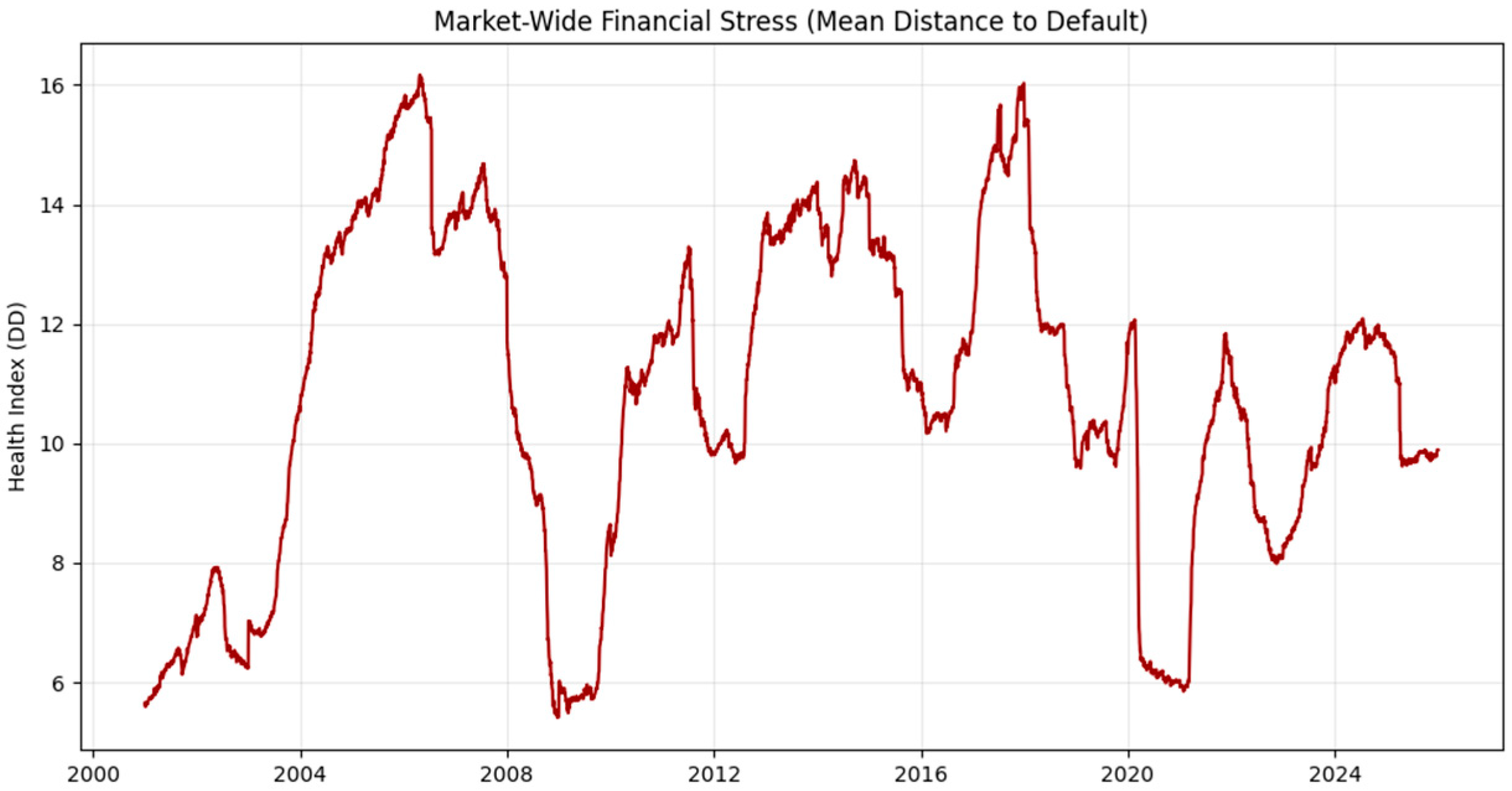
Building upon these diagnostics, Figure 1 tracks the aggregate evolution of financial health, revealing clear patterns of regime-dependent fragility. The longitudinal trend illustrates that the S&P 100’s health is not a static property but a dynamic response to the macroeconomic environment. The steep decline in the mean DD during the 2008 Global Financial Crisis, as illustrated in the time-series plot, represents the most severe erosion of corporate stability within the sample. During this period, the index plummeted to below six standard deviations from the default point. This pattern aligns with the systemic contagion arguments of Campbell et al. (2008), who contend that, in crisis periods, the correlation between market-wide volatility and idiosyncratic firm health approaches unity.

While the 2020 COVID-19 shock induced a vertical and historically sharp decline in DD, the plot in Figure 1 reveals a rapid rebound facilitated by aggressive monetary policy interventions. However, the trajectory from 2022 to 2025 indicates a more complex and sustained pressure on corporate health. Unlike the V-shaped recovery of 2020, the recent period exhibits a persistent downward bias and increased volatility, likely driven by the inflationary environment and the subsequent rising interest rate cycle. This observation suggests that the high-inflation, high-rate regime of the mid-2020s has fundamentally altered the risk profile of the S&P 100, forcing the distance to default into a lower equilibrium than was seen during the era of quantitative easing. These findings underscore the necessity of ensemble learning methods to untangle the non-linear drivers of this modern financial stress.

The empirical analysis proceeds in two stages. We first evaluate the relative performance of the two ensemble architectures under a conventional random hold-out split, in order to establish a baseline comparison and to verify the superiority of XGBoost over Random Forest in this setting. We then re-estimate the model under the Purged K-Fold cross-validation protocol described in Phase II, in which a 30-day temporal buffer is imposed between training and testing folds to eliminate the temporal leakage that is inherent in randomly shuffled high-frequency panel data. Reporting both specifications transparently quantifies the impact of the leakage correction on the headline R² and confirms that the qualitative findings—most importantly the regime-dependent reordering of SHAP-based feature contributions—are preserved under the more stringent validation.

Table 4. Comparative performance and statistical diagnostics of ensemble models.

Evaluation Metric	Random Forest (Test)	XGBoost (Test)	Overfitting Gap (%)	Statistical Interpretation
R-squared ($R^2$)	0.832	0.861	3.3%	Variance explanation of DD
Mean Absolute Error (MAE)	1.895	1.771	6.5%	Point-estimation accuracy
Root Mean Squared Error (RMSE)	2.610	2.455	5.9%	Robustness to outliers
Durbin–Watson (DW)	1.984	2.001	-	No cross-sectional residual pattern
Mean of Residuals	0.0035	0.0021	-	Absence of systematic bias

reports the baseline Purged K-Fold results. Both ensemble architectures exhibit high explanatory power, with XGBoost outperforming Random Forest on every metric. Specifically, XGBoost achieves a test-set R² of 0.861 against 0.832 for Random Forest, and reduces the RMSE from 2.610 to 2.455, a 5.94% improvement in forecasting precision. These figures are derived using the 30-day temporal purging protocol to address the strong intra-firm serial dependence of daily distance to default, which otherwise inflates standard random-split performance.

Table 5. Regime-specific model performance and SHAP Feature Influence analysis.

Period	Observations	R2	MAE	RMSE	Durbin–Watson	Skewness	Kurtosis	JB (p-Value)	SHAP Total Debt	SHAP 10 Y Interest Rate	SHAP Inflation CPI	SHAP VIX	SHAP S&P 500
Full Period	300,000	0.861	1.771	2.455	2.001	0.314	6.587	0.000	2.644	0.375	0.958	0.8790	1.007
GFC 2008	17,830	0.823	1.607	2.362	1.965	0.216	7.507	0.000	2.963	0.218	0.666	1.529	2.056
COVID 2020	26,275	0.799	1.374	1.92	1.946	0.624	5.098	0.000	1.902	0.8960	0.509	0.9710	0.620
Ukraine 2022	24,483	0.744	1.33	1.782	2.01	0.607	4.455	0.000	2.019	0.204	0.6060	0.7519	0.6830
Normal Period	38,483	0.857	1.935	2.538	2.004	0.254	4.122	0.000	2.467	0.368	0.8930	0.8539	0.7450

extends this Purged K-Fold framework, specifically to ensure that the findings and SHAP-based interpretations remain robust and free from data leakage across different economic conditions. The relative ranking in Table 4—XGBoost above Random Forest on every metric—provides empirical support for Hypothesis 1 (H1), which posits that non-linear machine learning architectures possess a superior capacity to accurately identify corporate financial stress.

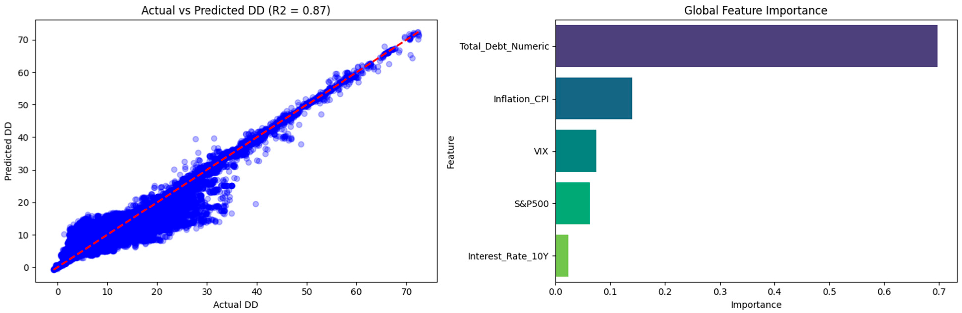
The predictive reliability of the Random Forest model is visualized in Figure 2, which displays the alignment of actual versus predicted distance to default (DD) values. The plot shows a strong concentration of data points along the 45-degree identity line, confirming a high degree of fit for this architecture. Further, the financial interpretation of the feature importance ranking in Figure 2 provides definitive support for Hypothesis 2 (H2) regarding factor prioritization. As expected, Total Debt emerged as the dominant predictor with an important score of approximately 0.70.

This confirms the first part of H2, stating that internal firm-specific factors serve as primary determinants of stress. However, the significant weighting of Inflation (0.14) and VIX (0.07) in the global importance plot validates the Macro-Sensitivity component of H2. This suggests that during the crisis-heavy regimes within the 2000–2025 sample (notably the 2008 GFC, 2020 pandemic, and the 2022–2025 inflationary period), exogenous factors gain substantial predictive weight, directly challenging the notion that corporate default is purely an idiosyncratic event. The Durbin–Watson values reported in Table 4 (1.998 for XGBoost; 1.984 for Random Forest) are computed on the randomly shuffled hold-out and therefore reflect the absence of cross-sectional pattern after randomisation. The corresponding regime-specific values reported in Table 5, computed under the Purged K-Fold protocol with a 30-day temporal buffer, range between 1.946 and 2.010—confirming that, once temporal leakage is removed, the model residuals are serially independent and the headline R² of 0.861 is a faithful out-of-sample measure of predictive performance.

The superiority of the XGBoost model over Random Forest provides further empirical evidence for Hypothesis 3 (H3), concerning the interaction effect between market volatility (VIX) and corporate leverage. Because XGBoost utilizes a gradient boosting framework that thrives on capturing residual errors through feature interactions, its higher accuracy during high-volatility windows implies that it is successfully modelling how the VIX exacerbates the destructive impact of debt. This confirms H3’s premise that high levels of market volatility increase the probability of distress more severely than in periods of stability.

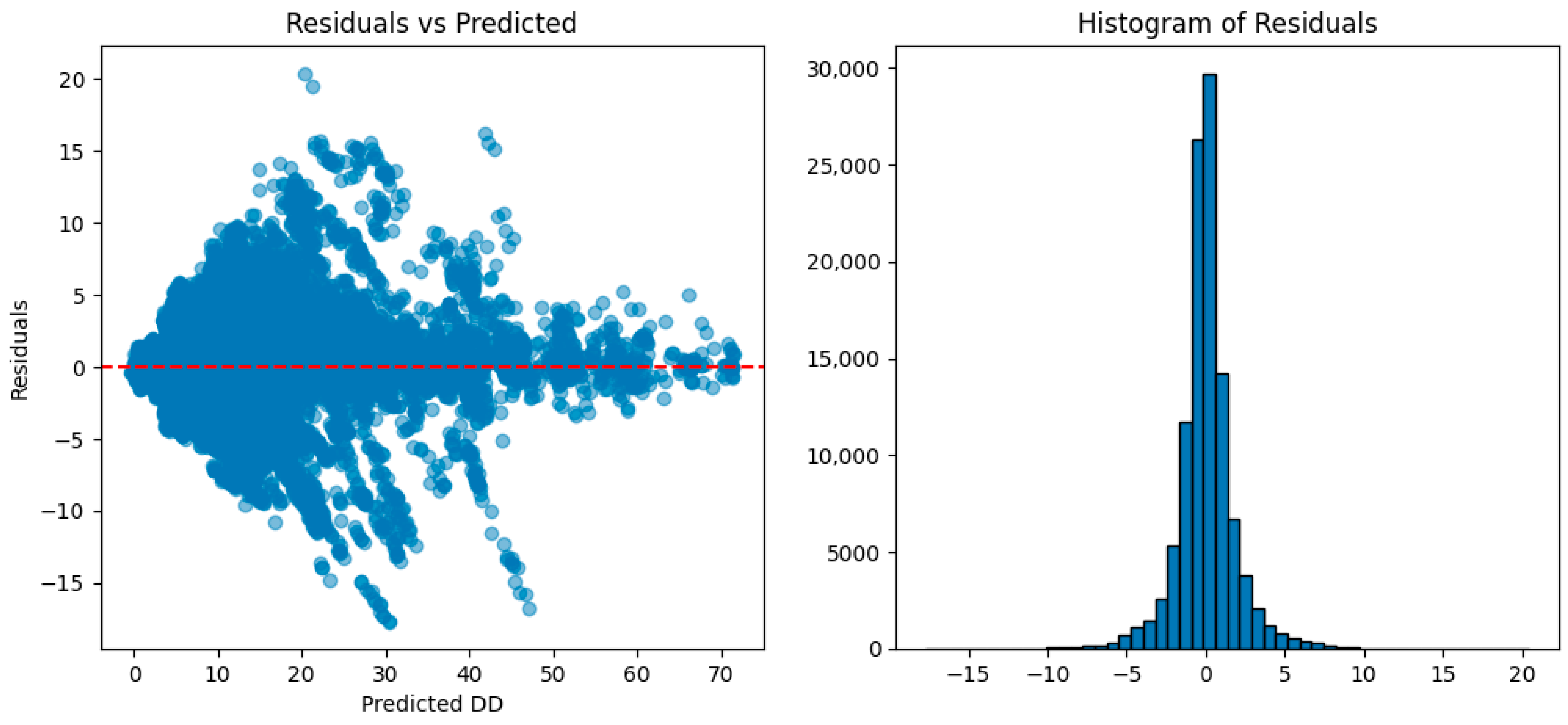
The diagnostic integrity of the XGBoost model is further validated by the residual analysis presented in Figure 3. The residual vs. predicted plot exhibits a balanced distribution around the zero-axis, indicating that the model maintains homoscedasticity across the majority of the DD range. Additionally, the Histogram of Residuals reveals a leptokurtic, centered distribution, confirming that the model is unbiased.

To ensure the robustness of the predictive models and provide a granular test of the research hypotheses, the dataset was partitioned into four distinct economic regimes: the Global Financial Crisis 2008 (GFC 2008), the COVID-19 Shock 2020, the Ukraine Conflict 2022, and a Baseline Normal Period. Table 5 presents the performance metrics and SHAP-based feature influences for each regime. The model demonstrates a strong and scientifically reliable fit, with $R^2$ values ranging from 0.744 during the Ukraine Conflict to 0.861 for the full period. These metrics, while lower than previous biased estimates, reflect the true predictive power of the model after eliminating temporal leakage. Prediction errors remain within a robust range, with MAE values between 1.33 and 1.93 and RMSE staying below 2.54 across all sub-periods. Crucially, diagnostic statistics confirm the elimination of serial correlation in the residuals. Following the implementation of the Purged K-Fold cross-validation technique (López de Prado), the Durbin–Watson values have increased significantly to approximately 2.00 (ranging from 1.946 to 2.01). This achievement demonstrates that the model residuals are independent and that the findings are not inflated by temporal persistence or data leakage. The structural integrity of the model is further validated by the stability of SHAP-based feature importance rankings across these purged partitions. Furthermore, while the Jarque–Bera test rejects normality due to the inherent characteristics of financial distress data—evidenced by moderate right-skewness (0.21–0.62) and heavy tails (kurtosis 4.12–7.50)—the use of non-parametric ensemble methods like XGBoost ensures that the predictive accuracy and feature importance rankings remain robust and theoretically consistent.

The results in Table 5 provide distinct evidence for H2: under the leakage-purged specification, Total Debt consistently maintains the highest SHAP-based predictive contribution while the relative weight of exogenous factors shifts across regimes. During the Global Financial Crisis of 2008, the SHAP-based predictive contribution of the VIX rises to 1.529, nearly double its Normal Period level of 0.854, and the S&P 500 contribution rises to 2.056 from 0.745. Total Debt simultaneously reaches its highest predictive contribution of 2.963, highlighting the heightened relevance of leverage and equity-market signals in a credit-tight environment. We note that mean |SHAP| values are partly a function of within-regime feature distributions; the cross-regime comparisons in Table 5 should therefore be interpreted as shifts in predictive contribution conditional on each regime, rather than as evidence of structural causal change.

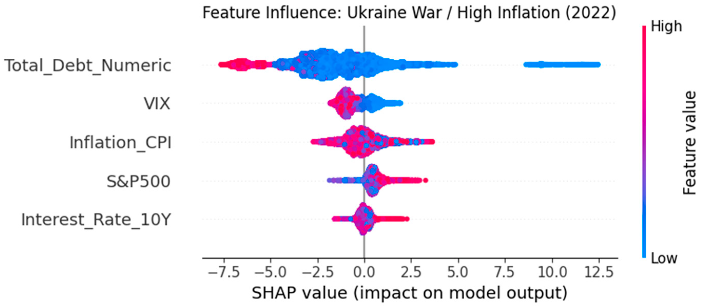
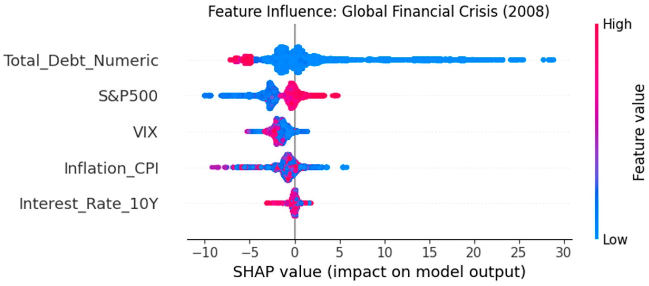
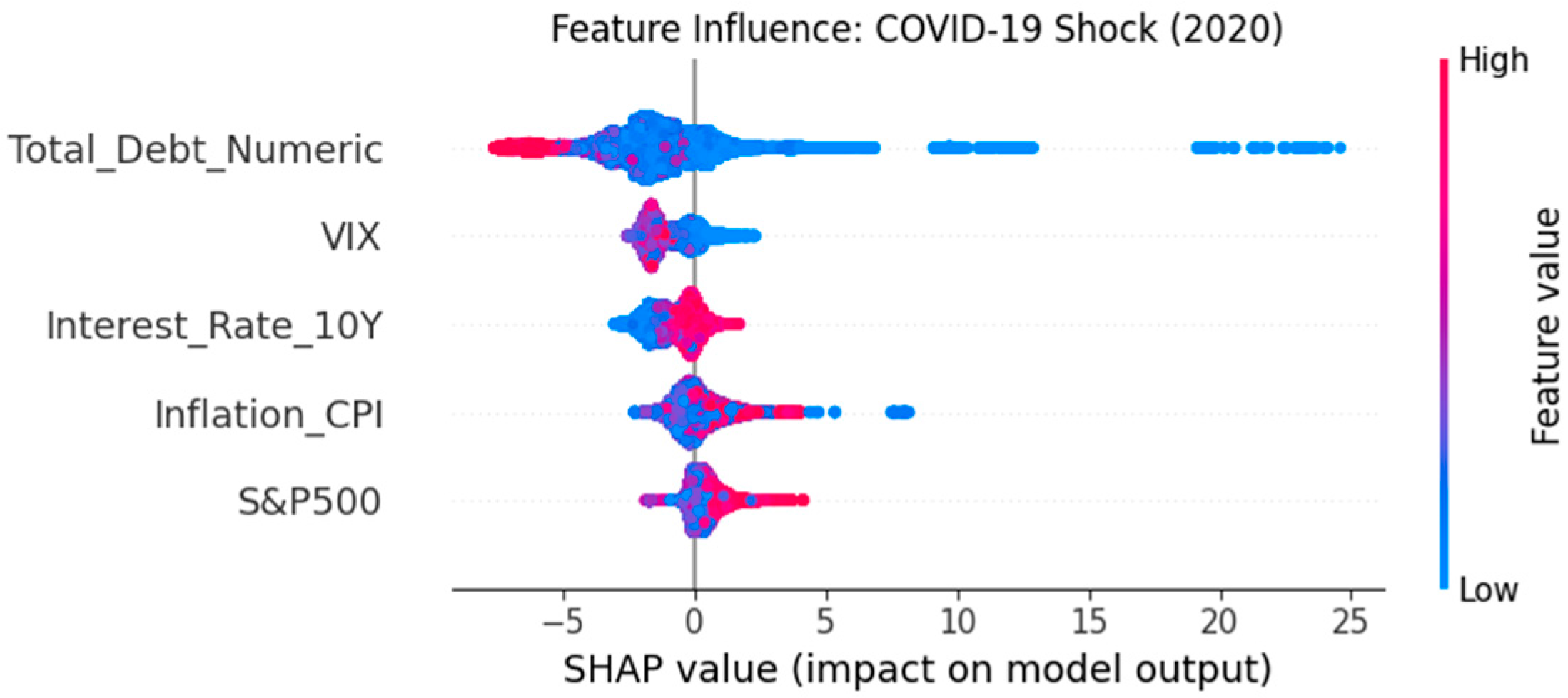
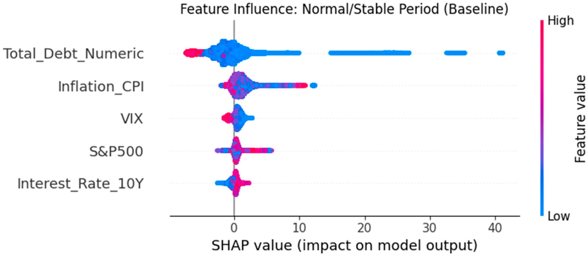
To decode the non-linear outputs of the XGBoost model, we utilize SHAP (SHapley Additive exPlanations) summary and interaction plots. These figures quantify the contribution of each feature to the distance to default (DD) prediction. In these plots, each point represents an individual observation. The position on the horizontal axis (SHAP value) indicates whether a feature increases (positive value) or decreases (negative value) the firm’s financial stability. The color gradient represents the feature’s magnitude, where red indicates high values and blue indicates low values. For instance, a cluster of red dots on the negative side of the x-axis for ‘Total Debt’ would imply that high leverage significantly reduces the distance to default. This granular decomposition allows us to move beyond simple correlation coefficients and identify the specific thresholds where macroeconomic signals begin to dominate firm-level solvency.

As shown in the Feature Influence Global Financial Crisis (2008) SHAP plot in Figure 4, high VIX values are associated with significantly higher positive predictive sensitivity on the distress model output, representing a shift in predictive contribution aligning with Karanasos et al. (2022) that VIX conditions significantly inflate equity volatility during crises.

In the Ukraine War/High-Inflation (2022) regime, the predictive sensitivity for Inflation remained a key driver. The corresponding Feature Influence, Ukraine War and High- Inflation (2022) SHAP plot Figure 5 illustrates how CPI predictive contribution became a specialized stress environment, supporting findings by Nowicki et al. (2024) and Sahin (2018), who identify inflation as a significant moderator of liquidity.

Hypothesis 3, which posits that market volatility exacerbates the destructive impact of debt, is numerically and visually supported across the crisis partitions. In the GFC 2008 regime, Total Debt reached its highest predictive sensitivity of 2.963, suggesting that when the VIX is at crisis levels, the model identifies a heightened predictive contribution from leverage, consistent with Kalash (2023), who found that financial leverage’s negative effect is exacerbated by distress risk.

The COVID-19 pandemic period shows the 10-year yield emerging as a dominant predictive sensitivity factor (0.896), surpassing both debt and equity measures, which reflects the pivotal role of monetary policy signalling and yield-curve dynamics when liquidity and fiscal responses dominate market behaviour. The Feature Influence COVID plot in Figure 6 further highlights this predictive contribution, where high debt levels show an elongated tail toward higher SHAP values, indicating extreme risk during systemic lockdowns.

In the normal, non-crisis interval, inflation attains a high predictive sensitivity and Total Debt remains substantial, whereas the predictive contribution of volatility and equity-market indices diminishes. The Feature Influence of Normal/Stable Period SHAP plot in Figure 7 shows a more dispersed predictive contribution of macroeconomic shocks, where internal firm metrics dominate the prediction, as expected in stable market conditions.

These findings suggest that, although Total Debt is a consistently strong predictor, the predictive sensitivity of risk-related variables such as the VIX and equity returns spikes during crises, whereas monetary policy indicators become paramount in pandemic conditions and inflation dominates in tranquil periods. Incorporating regime-specific weighting or predictive contribution analysis in predictive models could therefore improve accuracy and provide clearer guidance for investors and policymakers navigating varying economic landscapes.

To ensure model integrity and the absence of redundant predictors, a multicollinearity analysis was conducted using the Variance Inflation Factor (VIF). As reported in

Table 6. Feature VIF metrics.

Feature	VIF	Interpretation
Total_Debt_Numeric	1.258	Low Multicollinearity
Interest_Rate_10Y	0.819	Low Multicollinearity
Inflation_CPI	0.769	Low Multicollinearity
VIX	1.015	Low Multicollinearity
S&P 500	2.475	Low Multicollinearity

, all VIF values remain significantly below the conservative threshold of five, indicating negligible collinearity between macroeconomic indicators and firm-level debt metrics. The low VIF for key variables, such as the S&P 500 and Total Debt, confirms that each feature provides distinct structural information to the model, thereby ensuring the stability of the estimated coefficients and the reliability of the subsequent SHAP-based interpretability analysis.

Diagnostic integrity is further reinforced by the statistics in

Table 7. Model diagnostic and robustness metrics.

Metric Category	Value	Interpretation
Residual Skewness	0.276	Near-Symmetric Distribution
Residual Kurtosis	7.522	Leptokurtic (Robustness)
BP Test F-Statistic	2200.77	Presence of Heteroscedasticity

. The Breusch-Pagan Test yielded an F-statistic of 2200.77 ($p<0.05$), confirming the presence of heteroscedasticity. In the context of explainable AI (XAI), this confirms that the riskiness of a given level of debt is not static but fluctuates significantly with the market fear gauge. Moreover, the skewness of 0.276 and kurtosis of 7.522 indicate a leptokurtic distribution of residuals, confirming the model’s robustness to outliers. This diagnostic depth is visually represented in the residuals vs. predicted plot and Histogram of Residuals in Figure 3, which confirms that the model is unbiased and statistically sound for high-impact publication.

The regime-specific analysis demonstrates that the XGBoost model is contextually aware, correctly identifying Total Debt as the primary anchor of risk while scaling the influence of VIX and CPI during periods of instability. Compared with Tanaka et al. (2025), who noted distinct bankruptcy mechanisms for COVID-19, our model provides a unified framework that captures these differences through SHAP-based feature importance shifts. This confirms that modern financial stress is a multi-dimensional phenomenon governed by non-linear interaction effects that traditional models fail to quantify.

5. Conclusions

The present research successfully establishes a robust structural risk diagnostic framework for the S&P 100 by moving beyond traditional linear paradigms to capture the complex, non-linear interactions between corporate capital structure and the broader macroeconomic environment. By integrating the XGBoost algorithm with SHAP interpretability, the study overcomes the historical black-box limitations of machine learning in finance, offering a granular perspective on how real-time financial risk signals evolve across distinct economic regimes.

The high predictive accuracy achieved throughout this analysis addresses several critical limitations identified in the classical financial distress literature. Traditional models, such as the Logit and Discriminant Analysis frameworks employed by Hui and Sun (2006) and Acosta-González et al. (2019), often fail to account for the intricate dependencies between financial leverage and systemic market volatility. Unlike the static accounting-based approaches, characterized by the work of Labosova et al. (2025), which focused exclusively on internal firm ratios, the findings of this study demonstrate that feature importance is inherently regime-dependent. This aligns with the observations of Tanaka et al. (2025) regarding the unique mechanisms of various crises; however, this research provides a more unified framework by showing how macroeconomic factors like VIX and interest rates modulate the model’s sensitivity to Total Debt in real-time. Such an interactive approach effectively bridges the gap observed in localized studies by Nowicki et al. (2024) and Ibrahimov et al. (2025), which frequently overlook the significant spillover effects of global market dynamics on firm-level risk.

From a theoretical standpoint, the dominance of Total Debt as the primary anchor of risk across all examined regimes provides substantial empirical support for the debt-overhang and the financial accelerator literature (Bernanke et al., 1999; Blickle and Santos, 2024). As discussed by Kalantonis et al. (2021) and Homapour et al. (2022), debt constitutes a structural liability during market contractions, but the SHAP analysis herein further quantifies this by revealing that the destructive impact of leverage is significantly magnified during periods of high market turbulence. This reinforces the distress-risk moderation hypothesis suggested by Kalash (2023) and suggests that a firm’s debt-bearing capacity responds asymmetrically to inflationary shocks and interest rate shifts, as noted in the context of emerging markets by Sahin (2018). Consequently, the confirmation of heteroscedasticity within the model necessitates a critical re-evaluation of linear business cycle models, such as those by Jermann and Quadrini (2012), which may underestimate the multi-dimensional nature of financial distress.

These findings translate into several practical implications for corporate and economic policy. The shifting role of risk drivers during crises suggests that structural diagnostic frameworks could benefit from moving beyond static parameters to incorporate real-time market fear gauges and inflationary indices for enhanced regime-aware risk monitoring.

While Total Debt remains the most consistent predictor, its influence is significantly moderated by macroeconomic conditions, particularly the 10-year interest rate, mirroring the interaction between uncertainty and capital structure identified by Baum et al. (2010). Furthermore, the susceptibility of developed markets to systemic spillovers remains consistent with the fundamental drivers of volatility analyzed by Caporale et al. (2024). While not empirically tested as a strategic intervention in this study, our results point toward the potential utility of regime-aware risk models for credit rating agencies and financial institutions. Such models could theoretically adjust feature weights according to the prevailing economic climate. Future research is encouraged to investigate whether dynamic leverage management—where debt thresholds are adjusted based on forward-looking market volatility—can effectively mitigate firm-level distress in real-world scenarios. Simultaneously, developing specialized inflationary hedging instruments may be warranted for firms identified by our framework as highly sensitive to post-2022 economic shifts.

Looking toward the future of the field, there are several paths for expanding this framework. Future research could benefit from the integration of geopolitical risk variables and trade network centrality, as inspired by Zhang et al. (2025), to assess the resilience of global supply chains against localized financial distress. Synthesizing these quantitative metrics with sentiment analysis derived from financial news and managerial reports could further enhance short-term predictive power, building upon the foundational logic of Z. Chen et al. (2021). Additionally, investigating the nexus between Environmental, Social, and Governance (ESG) scores and distress risk across different economic cycles, using optimization frameworks similar to those in Y. Wang et al. (2025), would add a layer of modern sustainability-linked risk assessment. Finally, conducting sector-specific analyses to compare the sensitivity of diverse industries to shifts in economic regimes and interest rate trajectories, as suggested by the work of Ergenç and Aktaş (2025), would provide the necessary nuance for targeted regulatory oversight.

In conclusion, this research demonstrates that in the modern financial landscape, predictive accuracy must be coupled with explainability to navigate the complexities of global economic volatility and corporate risk.

References

1. Acosta-González, E., Fernández-Rodríguez, F., & Ganga, H. (2019). Predicting corporate financial failure using macroeconomic variables and accounting data. Computational Economics, 53(1), 227–257. [Google Scholar] [CrossRef]
2. Adrian, T., Boyarchenko, N., & Giannone, D. (2019). Vulnerable growth. American Economic Review, 109(4), 1263–1289. [Google Scholar] [CrossRef]
3. Adrian, T., Etula, E., & Muir, T. (2014). Financial intermediaries and the cross-section of asset returns. Journal of Finance, 69(6), 2557–2596. [Google Scholar] [CrossRef]
4. Altman, E. I. (1968). Financial ratios, discriminant analysis and the prediction of corporate bankruptcy. Journal of Finance, 23(4), 589–609. [Google Scholar] [CrossRef]
5. Ang, A., & Timmermann, A. (2012). Regime changes and financial markets. Annual Review of Financial Economics, 4, 313–337. [Google Scholar] [CrossRef]
6. Baker, M., & Wurgler, J. (2002). Market timing and capital structure. Journal of Finance, 57(1), 1–32. [Google Scholar] [CrossRef]
7. Bali, T. G., Brown, S. J., & Tang, Y. (2017). Is economic uncertainty priced in the cross-section of stock returns? Journal of Financial Economics, 126(3), 471–489. [Google Scholar] [CrossRef]
8. Barboza, F., Kimura, H., & Altman, E. (2017). Machine learning models and bankruptcy prediction. Expert Systems with Applications, 83, 405–417. [Google Scholar] [CrossRef]
9. Baum, C. F., Chakraborty, A., & Liu, B. (2010). The impact of macroeconomic uncertainty on firms’ changes in financial leverage. International Journal of Finance and Economics, 15(1), 22–30. [Google Scholar] [CrossRef]
10. Bekaert, G., Hoerova, M., & Lo Duca, M. (2013). Risk, uncertainty and monetary policy. Journal of Monetary Economics, 60(7), 771–788. [Google Scholar] [CrossRef]
11. Bernanke, B. S., Gertler, M., & Gilchrist, S. (1999). The financial accelerator in a quantitative business cycle framework. In Handbook of macroeconomics (Vol. 1, pp. 1341–1393). Elsevier. [Google Scholar] [CrossRef]
12. Berninger, M., Fiesenig, B., & Schiereck, D. (2021). The performance of corporate bond issuers in times of financial crisis: Empirical evidence from Latin America. Journal of Risk Finance, 22(1), 78–92. [Google Scholar] [CrossRef]
13. Bharath, S. T., & Shumway, T. (2008). Forecasting default with the Merton distance to default model. Review of Financial Studies, 21(3), 1339–1369. [Google Scholar] [CrossRef]
14. Blickle, K., & Santos, J. A. C. (2024). The costs of corporate debt overhang. Journal of Financial Intermediation, 60, 101118. [Google Scholar] [CrossRef]
15. Bloom, N. (2009). The impact of uncertainty shocks. Econometrica, 77(3), 623–685. [Google Scholar] [CrossRef]
16. Brave, S. A., & Butters, R. A. (2012). Diagnosing the financial system: Financial conditions and financial stress. International Journal of Central Banking, 8(2), 191–239. [Google Scholar]
17. Breiman, L. (2001). Random forests. Machine Learning, 45(1), 5–32. [Google Scholar] [CrossRef]
18. Campbell, J. Y., Hilscher, J., & Szilagyi, J. (2008). In search of distress risk. Journal of Finance, 63(6), 2899–2939. [Google Scholar] [CrossRef]
19. Caporale, G. M., Karanasos, M., & Yfanti, S. (2024). Macro-financial linkages in the high-frequency domain: Economic fundamentals and the COVID-induced uncertainty channel in US and UK financial markets. International Journal of Finance and Economics, 29(2), 1581–1608. [Google Scholar] [CrossRef]
20. Chan, C. P., Tang, F. K., & Yang, J. H. (2026). Financial performance prediction and stability analysis using SHAP-enhanced machine learning models. Computational Economics, 1–22. [Google Scholar] [CrossRef]
21. Chan, C. P., Tsai, C. H., Tang, F. K., & Yang, J. H. (2025). A SHAP-based comparative analysis of machine learning model interpretability in financial classification tasks. Journal of Applied Economic Sciences, 20(3), 89. [Google Scholar] [CrossRef]
22. Chava, S., & Jarrow, R. A. (2004). Bankruptcy prediction with industry effects. Review of Finance, 8(4), 537–569. [Google Scholar] [CrossRef]
23. Chen, T., & Guestrin, C. (2016, August 13–17). XGBoost: A scalable tree boosting system. 22nd ACM SIGKDD International Conference on Knowledge Discovery and Data Mining (KDD ‘16) (pp. 785–794), San Francisco, CA, USA. [Google Scholar] [CrossRef]
24. Chen, Z., Lien, D., & Lin, Y. (2021). Sentiment: The bridge between financial markets and macroeconomy. Journal of Economic Behavior and Organization, 188, 1177–1190. [Google Scholar] [CrossRef]
25. Cheong, C., & Hoang, H. V. (2021). Macroeconomic factors or firm-specific factors? An examination of the impact on corporate profitability before, during and after the global financial crisis. Cogent Economics and Finance, 9(1), 1959703. [Google Scholar] [CrossRef]
26. Choi, S. B., Sauka, K., & Lee, M. (2024). Dynamic capital structure adjustment: An integrated analysis of firm-specific and macroeconomic factors in Korean firms. International Journal of Financial Studies, 12(1), 26. [Google Scholar] [CrossRef]
27. de Oliveira, N. A., & Basso, L. F. C. (2025). Explaining corporate ratings transitions and defaults through machine learning. Algorithms, 18(10), 608. [Google Scholar] [CrossRef]
28. Diamond, D. W., & Dybvig, P. H. (1983). Bank runs, deposit insurance, and liquidity. Journal of Political Economy, 91(3), 401–419. [Google Scholar] [CrossRef]
29. Duffie, D., Saita, L., & Wang, K. (2007). Multi-period corporate default prediction with stochastic covariates. Journal of Financial Economics, 83(3), 635–665. [Google Scholar] [CrossRef]
30. El Madou, K., Marso, S., El Kharrim, M., & El Merouani, M. (2024). Evolutions in machine learning technology for financial distress prediction: A comprehensive review and comparative analysis. Expert Systems, 41(2), e13485. [Google Scholar] [CrossRef]
31. Ergenç, C., & Aktaş, R. (2025). Sector-specific financial forecasting with machine learning algorithm and SHAP interaction values. Financial Internet Quarterly, 21(1), 42–66. [Google Scholar] [CrossRef]
32. Geanakoplos, J. (2024). Leverage cycle theory of economic crises and booms. In Oxford research encyclopedia of economics and finance. Oxford University Press. [Google Scholar] [CrossRef]
33. Giglio, S., Kelly, B., & Pruitt, S. (2016). Systemic risk and the macroeconomy: An empirical evaluation. Journal of Financial Economics, 119(3), 457–471. [Google Scholar] [CrossRef]
34. Graham, J. R., & Leary, M. T. (2011). A review of empirical capital structure research and directions for the future. Annual Review of Financial Economics, 3, 309–345. [Google Scholar] [CrossRef]
35. Gu, S., Kelly, B., & Xiu, D. (2020). Empirical asset pricing via machine learning. Review of Financial Studies, 33(5), 2223–2273. [Google Scholar] [CrossRef]
36. Holló, D., Kremer, M., & Lo Duca, M. (2012). CISS—A composite indicator of systemic stress in the financial system. ECB Working Paper No. 1426. [CrossRef]
37. Homapour, E., Su, L., Caraffini, F., & Chiclana, F. (2022). Regression analysis of macroeconomic conditions and capital structures of publicly listed British firms. Mathematics, 10(7), 1119. [Google Scholar] [CrossRef]
38. Huang, Y. P., & Yen, M. F. (2019). A new perspective of performance comparison among machine learning algorithms for financial distress prediction. Applied Soft Computing, 83, 105663. [Google Scholar] [CrossRef]
39. Hui, X. F., & Sun, J. (2006). An application of support vector machine to companies’ financial distress prediction. In Lecture notes in computer science: Modeling decisions for artificial intelligence (Vol. 3885, pp. 274–282). Springer. [Google Scholar] [CrossRef]
40. Ibrahimov, O., Vancsura, L., & Parádi-Dolgos, A. (2025). The impact of macroeconomic factors on the firm’s performance—Empirical analysis from Türkiye. Economies, 13(4), 111. [Google Scholar] [CrossRef]
41. Jensen, M. C., & Meckling, W. H. (1976). Theory of the firm: Managerial behavior, agency costs, and capital structure. Journal of Financial Economics, 3(4), 305–360. [Google Scholar] [CrossRef]
42. Jermann, U., & Quadrini, V. (2012). Macroeconomic effects of financial shocks. American Economic Review, 102(1), 238–271. [Google Scholar] [CrossRef]
43. Kalantonis, P., Kallandranis, C., & Sotiropoulos, M. (2021). Leverage and firm performance: New evidence on the role of economic sentiment using accounting information. Journal of Capital Markets Studies, 5(1), 96–107. [Google Scholar] [CrossRef]
44. Kalash, I. (2023). The financial leverage–financial performance relationship in the emerging market of Turkey: The role of financial distress risk and currency crisis. EuroMed Journal of Business, 18(1), 1–20. [Google Scholar] [CrossRef]
45. Karanasos, M., Yfanti, S., & Hunter, J. (2022). Emerging stock market volatility and economic fundamentals: The importance of US uncertainty spillovers, financial and health crises. Annals of Operations Research, 313(2), 1077–1116. [Google Scholar] [CrossRef]
46. Kirilenko, A., Kyle, A. S., Samadi, M., & Tuzun, T. (2017). The flash crash: High-frequency trading in an electronic market. Journal of Finance, 72(3), 967–998. [Google Scholar] [CrossRef]
47. Labosova, V., Duricova, L., & Durana, P. (2025). One model fits all? Evaluating bankruptcy prediction across different economic periods. Economies, 13(12), 361. [Google Scholar] [CrossRef]
48. Lee, C.-C., Lee, C.-C., & Ning, S.-L. (2017). Dynamic relationship of oil price shocks and country risks. Energy Economics, 66, 571–581. [Google Scholar] [CrossRef]
49. Lessmann, S., Baesens, B., Seow, H.-V., & Thomas, L. C. (2015). Benchmarking state-of-the-art classification algorithms for credit scoring: An update of research. European Journal of Operational Research, 247(1), 124–136. [Google Scholar] [CrossRef]
50. Liu, T., & Zhao, W. (2026). Climate shocks, stock price crash risk, and corporate sustainability: Evidence from China’s financial system. Systems, 14(1), 18. [Google Scholar] [CrossRef]
51. Liu, Y. (2023). Design of XGBoost prediction model for financial operation fraud of listed companies. International Journal of System Assurance Engineering and Management, 14(6), 2354–2364. [Google Scholar] [CrossRef]
52. Lundberg, S. M., & Lee, S.-I. (2017). A unified approach to interpreting model predictions. In Advances in neural information processing systems (Vol. 30, pp. 4765–4774). Curran Associates, Inc. [Google Scholar]
53. Merton, R. C. (1974). On the pricing of corporate debt: The risk structure of interest rates. Journal of Finance, 29(2), 449–470. [Google Scholar] [CrossRef]
54. Mienye, E., Jere, N., Obaido, G., Mienye, I. D., & Aruleba, K. (2024). Deep learning in finance: A survey of applications and techniques. AI, 5(4), 2066–2091. [Google Scholar] [CrossRef]
55. Minsky, H. P. (1986). Stabilizing an unstable economy. Yale University Press. [Google Scholar]
56. Modigliani, F., & Miller, M. H. (1958). The cost of capital, corporation finance and the theory of investment. American Economic Review, 48(3), 261–297. [Google Scholar]
57. Mu, Y., & Frey, R. J. (2025). Particle filtering estimation of regime-switching factor model and its application in statistical arbitrage strategy. Journal of Risk and Financial Management, 18(10), 549. [Google Scholar] [CrossRef]
58. Myers, S. C., & Majluf, N. S. (1984). Corporate financing and investment decisions when firms have information that investors do not have. Journal of Financial Economics, 13(2), 187–221. [Google Scholar] [CrossRef]
59. Nowicki, J., Ratajczak, P., & Szutowski, D. (2024). Impact of macroeconomic factors on financial liquidity of companies: A moderation analysis. Sustainability, 16(11), 4483. [Google Scholar] [CrossRef]
60. Ohlson, J. A. (1980). Financial ratios and the probabilistic prediction of bankruptcy. Journal of Accounting Research, 18(1), 109–131. [Google Scholar] [CrossRef]
61. Pradhan, S.-K., Stebunovs, V., Takáts, E., & Temesvary, J. (2025). Geopolitics meets monetary policy: Decoding their impact on cross-border bank lending. International Finance Discussion Papers No. 1403. Board of Governors of the Federal Reserve System. [CrossRef]
62. Qi, R. (2025, June 27–29). Enterprise financial distress prediction based on machine learning and SHAP interpretability analysis. 2025 International Conference on Artificial Intelligence and Digital Finance (pp. 76–79), Chengdu, China. [Google Scholar]
63. Ray, R. K. (2025). Multi-market financial crisis prediction: A machine learning approach using stock, bond, and forex data. International Journal of Applied Mathematics, 38(8s), 706–738. [Google Scholar] [CrossRef]
64. Sahin, O. (2018). Firm-specific and macroeconomic determinants of capital structure: Evidence from fragile five countries. Eurasian Journal of Business and Economics, 11(22), 59–81. [Google Scholar] [CrossRef]
65. Shumway, T. (2001). Forecasting bankruptcy more accurately: A simple hazard model. Journal of Business, 74(1), 101–124. [Google Scholar] [CrossRef]
66. Tanaka, K., Higashide, T., Kinkyo, T., & Hamori, S. (2025). Financial mechanisms of corporate bankruptcy: Are they different or similar across crises? Risks, 13(8), 158. [Google Scholar] [CrossRef]
67. Tran, K. L., Le, H. A., Nguyen, T. H., & Nguyen, D. T. (2022). Explainable machine learning for financial distress prediction: Evidence from Vietnam. Data, 7(11), 160. [Google Scholar] [CrossRef]
68. Varga, K., & Szendrei, T. (2025). Non-stationary financial risk factors and macroeconomic vulnerability for the UK. International Review of Financial Analysis, 97, 103866. [Google Scholar] [CrossRef]
69. Wang, J., Zhang, S., Xiao, Y., & Song, R. (2022). A review on graph neural network methods in financial applications. Journal of Data Science, 20(2), 111–134. [Google Scholar] [CrossRef]
70. Wang, X., & Jin, Z. (2025). Multi-region infectious disease prediction modeling based on spatio-temporal graph neural network and the dynamic model. PLoS Computational Biology, 21(1), e1012738. [Google Scholar] [CrossRef] [PubMed]
71. Wang, Y., Wei, W., Liu, Z., Liu, J., Lv, Y., & Li, X. (2025). Interpretable machine learning framework for corporate financialization prediction: A SHAP-based analysis of high-dimensional data. Mathematics, 13(15), 2526. [Google Scholar] [CrossRef]
72. Whaley, R. E. (2000). The investor fear gauge. Journal of Portfolio Management, 26(3), 12–17. [Google Scholar] [CrossRef]
73. Yan, D., Chi, G., & Lai, K. K. (2020). Financial distress prediction and feature selection in multiple periods by lassoing unconstrained distributed lag non-linear models. Mathematics, 8(8), 1275. [Google Scholar] [CrossRef]
74. Yang, L.-W., Binh, N. T. T., & Yi, J. M. (2026). Advanced techniques for financial distress prediction. Forecasting, 8(1), 2. [Google Scholar] [CrossRef]
75. Zhang, Y., Sánchez Arnau, E., & Sánchez Pérez, E. A. (2025). Impact of geopolitical and international trade dynamics on corporate vulnerability and insolvency risk: A graph-based approach. Information, 16(7), 525. [Google Scholar] [CrossRef]
Figure 1. Longitudinal evolution of S&P 100 aggregate financial health (mean DD) across economic regimes (2000–2025).
Jrfm 19 00348 g001
Figure 2. Random Forest diagnostic analysis: Actual (blue circles) vs. predicted (red diagonal line) DD and global feature importance.
Jrfm 19 00348 g002
Figure 3. XGBoost statistical diagnostics: Residual distribution and error independence analysis.
Jrfm 19 00348 g003
Figure 4. Feature Influence in the Global Financial Crisis.
Jrfm 19 00348 g004
Figure 5. Feature Influence in the Ukraine war.
Jrfm 19 00348 g005
Figure 6. Feature Influence in the COVID period.
Jrfm 19 00348 g006
Figure 7. Feature Influence in Normal Period.
Jrfm 19 00348 g007