Functional Similarity of Financial Trajectories for Corporate Bankruptcy Prediction: A k-Nearest Neighbors Approach

Abstract

Corporate risk prediction is a central problem in financial analysis and corporate risk management. This study proposes a functional approach in which firms are represented through multivariate financial trajectories constructed from retrospective windows of accounting indicators, over which a similarity measure is defined and incorporated into a k-nearest neighbors classifier. The target variable is derived from administrative records, combining reporting discontinuity and firm administrative status as a proxy for financial distress. The empirical application is conducted using data from firms in the tourism sector in Colombia and is evaluated through stratified cross-validation. The results show that the trajectory-based representation captures gradual patterns of financial deterioration and improves the performance of k-NN relative to its static variable counterpart. In addition, the approach enhances interpretability by enabling the identification of historically comparable firms and the analysis of the financial dimensions that explain their similarity. Overall, the model provides a complementary perspective for corporate risk analysis based on the comparison of financial trajectories.

1. Introduction

The prediction of corporate bankruptcy risk is a central topic in financial research and corporate risk management (Dasilas & Rigani, 2024; Zhao et al., 2024). The failure of a firm can generate significant effects on creditors, employees, and markets, which is why the development of tools capable of early detection of financial distress signals has been a persistent concern in both the academic literature and professional practice (Graham et al., 2023). In addition to predictive capability, in many contexts it is also relevant to have tools that allow the comparison of a firm’s financial evolution with that of other firms that have experienced similar trajectories (Li et al., 2022).

Recent developments in machine learning methods have significantly expanded the tools available to address this problem. In particular, the literature has incorporated techniques such as neural networks, support vector machines, decision trees, random forests, and various ensemble methods, with the aim of improving the predictive performance of traditional models (Dasilas & Rigani, 2024; Zhao et al., 2024).

Despite these advances, the growing predominance of increasingly complex models has also raised important challenges in terms of interpretability. Many of the approaches that currently dominate the literature, such as neural networks, support vector machines, or boosting models (e.g., XGBoost, LightGBM, or CatBoost), have demonstrated a remarkable ability to identify patterns associated with bankruptcy risk. However, these methods typically operate as black-box systems, in which it is difficult to directly understand the mechanisms that lead to a given prediction (Carmona et al., 2022; Černevičienė & Kabašinskas, 2024; Yeo et al., 2025).

To address this limitation, several studies have proposed post-hoc interpretability tools, such as SHAP or LIME (Lundberg & Lee, 2017; Ribeiro et al., 2016), which allow for approximating the contribution of variables to the predictions generated by these models. However, these strategies act as external explanation mechanisms and are not intrinsically part of the model’s decision process. In contexts such as financial analysis and risk management, where the interpretation of results can be as relevant as predictive accuracy, this limitation has motivated the search for approaches that combine competitive performance with more transparent decision structures (Carmona et al., 2022; Cho & Shin, 2023; Crosato et al., 2023; Lin et al., 2025).

In this context, nearest-neighbor methods constitute a naturally interpretable alternative. In particular, the k-Nearest Neighbors (k-NN) algorithm classifies new observations based on their similarity to previously observed cases, so that each prediction can be explained through the identification of comparable historical units. This feature is especially valuable in financial analysis, where the ability to relate a firm to others with similar behavior can facilitate the economic interpretation of results (Barceló et al., 2025; Li et al., 2022).

However, despite this conceptual advantage, the use of k-NN has been relatively limited in the recent bankruptcy prediction literature. Several comparative studies show that, when evaluated alongside other machine learning algorithms, its predictive performance tends to be lower than that of more complex models based on ensembles, boosting, or deep learning architectures (Smiti & Soui, 2020).

Beyond its relatively lower performance, an important limitation of the k-NN approach in this context is related to the way financial information is represented. In its standard formulation, the algorithm is typically applied to vectors of indicators observed in a single period, so that each firm is described as a static observation (Zhao et al., 2024). However, financial distress rarely occurs abruptly. In practice, it usually manifests as a gradual process that unfolds over time, reflected in persistent changes in financial indicators (Abrahamsen et al., 2024; Zhou et al., 2022).

In this line, the literature has addressed the analysis of corporate risk through formulations that explicitly incorporate the temporal dimension or redefine the event of interest. These approaches include, among others, models that consider the recurrence of financial distress and representations based on the evolution of indicators over time (Abrahamsen et al., 2024; Zhou et al., 2022). Taken together, these developments suggest that the identification of firms at risk can be approached beyond the traditional static representation by incorporating the temporal dynamics of financial information.

Based on this, the present study proposes a functional approach to the analysis of corporate bankruptcy risk. Instead of representing firms as isolated firm–year observations, the developed framework models each firm based on the recent evolution of its financial indicators using retrospective windows (Sabri et al., 2025; Zhou et al., 2022). On this representation, a similarity measure is defined to compare multivariate financial trajectories (Wang et al., 2024).

From this formulation, a functional k-Nearest Neighbors model is developed, allowing the identification of neighborhoods of firms with comparable financial trajectories and the estimation of risk based on the observed evolution of historically similar firms (Li et al., 2022; Sabri et al., 2025). In this sense, the approach does not seek to replace more complex models that currently dominate the literature, but rather to provide a complementary perspective based on the comparison of financial trajectories.

The empirical application is conducted on firms in the tourism sector in Colombia, which allows illustrating how the identification of similar financial trajectories can provide relevant information for corporate risk analysis and management (Dioko & Guo, 2024).

2. Materials and Methods

This section describes the methodological approach proposed for the analysis of corporate financial distress risk based on multivariate financial trajectories. The model is conceived as an integrated system composed of four interrelated elements: (i) a functional representation of recent accounting information, (ii) the construction of a target variable that captures conditions of deterioration and business discontinuity ($RQ$), (iii) a functional metric specifically designed to compare financial dynamics over time, and (iv) a classifier based on nearest neighbors (k-NN). This variable should not be interpreted as a direct measure of legal bankruptcy, but rather as an operational proxy for financial distress based on information observed in administrative records.

In this context, the objective of the approach is not only to assign a risk classification, but also to identify historically comparable firms based on their recent financial trajectories and to use this information as a basis for risk interpretation and the analysis of deterioration patterns. Therefore, the problem is formulated as a trajectory classification task rather than as a traditional prediction exercise in a firm–year structure.

The components of the model are presented sequentially as follows. The section begins with a description of the dataset and the construction of financial trajectories, followed by the definition of the target variable, the formulation of the functional metric, and, finally, the implementation and evaluation of the classifier.

2.1. Data, Cleaning, and Accounting Imputation

The data are obtained from the annual financial statements reported by Colombian firms to the Superintendence of Companies, the national authority responsible for corporate supervision, and downloaded from the Integrated Corporate Information System (SIIS). The dataset covers the period 1995–2023 and includes firms from multiple economic sectors.

The analysis is restricted to firms belonging to the tourism sector, identified based on the CIIU classification.

Given that accounting formats and frameworks change over time, particularly with the adoption of IFRS starting in 2016, a standardization procedure was implemented to consolidate and harmonize the different historical files. This process involved the alignment of accounting accounts that, although representing the same economic reality, may differ in their denomination, classification, or structure across periods. In this way, the intertemporal consistency of the main accounts in the balance sheet, income statement, and cash flow statement is ensured.

As a preliminary stage, a structural data cleaning process was conducted to ensure the accounting consistency of the information. This process included verifying the temporal consistency of the data, the availability of the required financial statements, and the validation of basic accounting identities (e.g., the equality between assets, liabilities, and equity).

Additionally, the consistency of the firm identifier (NIT) was verified across the different financial statements within the same year, with minor inconsistencies corrected when necessary. Finally, duplicate records were removed to ensure a single observation per firm–year.

To guarantee the completeness of the variables required for the calculation of financial indicators, an imputation scheme was implemented based exclusively on explicit accounting rules and economic coherence, ensuring that all transformations are fully reproducible from the original information.

First, accounts with missing values that can be interpreted as an absence of activity were imputed with zero (e.g., inventories, accounts receivable/payable, financial expenses, administrative and selling expenses, depreciation and amortization, and free cash flow), thereby avoiding the introduction of inconsistencies in accounting identities.

Second, derivable accounts, such as net income, EBIT, gross profit, or taxes, were reconstructed from verifiable accounting relationships when sufficient information was available (e.g., imputing net income as the difference between EBIT and taxes).

Finally, when residual missing values persisted, these were imputed with zero only in cases where the same firm (NIT) had reported that account in other periods, using historical evidence as support. Automatic statistical imputation methods (such as MICE, k-NN, or regressions) were not used, as they may generate combinations that do not preserve the structural coherence of financial statements.

After applying the accounting rule-based imputation procedures, a small fraction of observations still presented missing values in key financial accounts. These cases, representing approximately 1.18% of the dataset, correspond to firms with insufficient information that could not be reconstructed under consistent accounting criteria.

For this reason, these observations were excluded from the analysis, reducing the number of firms from 5839 to 5770 and the number of firm–year observations from 52,720 to 52,575. Given that this proportion is marginal, their exclusion does not compromise the representativeness of the dataset or the validity of the empirical results.

2.2. Construction of Financial Indicators

An initial set of 45 financial indicators was constructed from the available accounting data. These indicators include standard ratios capturing different dimensions of firm performance, such as liquidity, leverage, coverage, and profitability, and were computed directly from the cleaned accounting information, preserving the economic interpretation of the underlying variables.

The construction of this broad set of indicators aims to provide a structured representation of firms’ financial information in each period.

This set constitutes the basis for its subsequent use in the analysis of financial trajectories, allowing for a consistent characterization of the temporal evolution of each firm.

Given the high degree of redundancy and multicollinearity characteristic of financial indicators, a structured dimensionality reduction procedure was implemented. In particular, a hierarchical clustering method based on the matrix of absolute correlations was applied, with the objective of identifying groups of indicators exhibiting highly similar behavior.

Clustering was performed using Ward’s method on previously standardized variables, which allows indicators to be compared on a common scale without altering their structural relationships. For this stage only, missing and infinite values were temporarily handled to ensure the numerical stability of the clustering algorithm. This treatment does not alter the economic structure of the data nor the way indicators are subsequently used in the model.

From each identified cluster, a representative indicator was selected based on the lowest Variance Inflation Factor (VIF), with the aim of minimizing multicollinearity in the final set.

This selection does not correspond to a removal strategy aimed at maximizing predictive performance, but rather to the identification of a representative variable for each group of highly correlated indicators, such that each retained variable summarizes the information of a set of indicators with equivalent behavior.

As a result, a reduced set of 17 financial indicators was obtained, which are used in the empirical analysis.

It is important to emphasize that this selection does not aim to identify individually predictive variables, but rather to construct a parsimonious and coherent representation of financial information that serves as the basis for building comparable trajectories across firms.

No winsorization techniques or additional transformations of extreme values were applied, as these, including infinite values, arise naturally from accounting relationships and form part of the economic structure of the data.

Table 1. Selected financial indicators, exact formulas, and case-handling rules implemented in the code.

Code	Name	Formula	Case Handling
RA	Asset Turnover	$RA={\displaystyle \frac{V}{AT}}$	$\begin{array}{c}V=0\wedge AT=0\Rightarrow \mathrm{NaN}\hfill \\ AT=0\wedge V>0\Rightarrow +\infty \hfill \end{array}$
RCID	Debt Coverage with Interest	$RCID={\displaystyle \frac{EBIT+GF}{PT}}$	$\begin{array}{c}(EBIT+GF)=0\wedge PT=0\Rightarrow \mathrm{NaN}\hfill \\ PT=0\wedge (EBIT+GF)>0\Rightarrow +\infty \hfill \end{array}$
RAF	Financial Leverage Ratio	$RAF={\displaystyle \frac{AF}{PN}}$	$\begin{array}{c}AF=0\wedge PN=0\Rightarrow \mathrm{NaN}\hfill \\ PN=0\wedge AF>0\Rightarrow +\infty \hfill \end{array}$
MO	Operating Margin	$MO={\displaystyle \frac{UO}{V}}$	$\begin{array}{c}UO=0\wedge V=0\Rightarrow \mathrm{NaN}\hfill \\ V=0\wedge UO>0\Rightarrow +\infty \hfill \end{array}$
PPP	Average Payment Period	$PPP={\displaystyle \frac{CPP}{V/365}}$	$\begin{array}{c}CPP=0\wedge V=0\Rightarrow \mathrm{NaN}\hfill \\ V=0\wedge CPP>0\Rightarrow +\infty \hfill \end{array}$
LG	General Liquidity	$LG={\displaystyle \frac{AC+AF}{PCP}}$	$\begin{array}{c}(AC+AF)=0\wedge PCP=0\Rightarrow \mathrm{NaN}\hfill \\ PCP=0\wedge (AC+AF)>0\Rightarrow +\infty \hfill \end{array}$
T	Treasury Ratio	$T={\displaystyle \frac{AC-I}{PT}}$	$\begin{array}{c}(AC-I)=0\wedge PT=0\Rightarrow \mathrm{NaN}\hfill \\ PT=0\wedge (AC-I)>0\Rightarrow +\infty \hfill \end{array}$
ROE	Return on Equity	$ROE={\displaystyle \frac{UN}{PN}}$	$\begin{array}{c}UN=0\wedge PN=0\Rightarrow \mathrm{NaN}\hfill \\ PN=0\wedge UN>0\Rightarrow +\infty \hfill \end{array}$
KTNO	Net Operating Working Capital	$KTNO=CPC+I-CPP$	$\begin{array}{c}\mathrm{All}\mathrm{missing}\Rightarrow \mathrm{NaN}\hfill \\ \mathrm{Missing}CPC,I\Rightarrow -CPP\hfill \\ \mathrm{Missing}CPP\Rightarrow CPC+I\hfill \end{array}$
MB	Gross Margin	$MB={\displaystyle \frac{UB}{V}}$	$\begin{array}{c}UB=0\wedge V=0\Rightarrow \mathrm{NaN}\hfill \\ V=0\wedge UB>0\Rightarrow +\infty \hfill \end{array}$
AFT	Fixed Assets over Total Financing	$AFT={\displaystyle \frac{AF+PT}{AF+PN}}$	$\begin{array}{c}(AF+PT)=0\wedge (AF+PN)=0\Rightarrow \mathrm{NaN}\hfill \\ (AF+PN)=0\wedge (AF+PT)>0\Rightarrow +\infty \hfill \\ (AF+PT)=0\wedge (AF+PN)>0\Rightarrow 0\hfill \end{array}$
RI	Inventory Turnover	$RI={\displaystyle \frac{V}{I}}$	$\begin{array}{c}V=0\wedge I=0\Rightarrow \mathrm{NaN}\hfill \\ I=0\wedge V>0\Rightarrow +\infty \hfill \end{array}$
RCC	Accounts Receivable Turnover	$RCC={\displaystyle \frac{V}{CPC}}$	$\begin{array}{c}V=0\wedge CPC=0\Rightarrow \mathrm{NaN}\hfill \\ CPC=0\wedge V>0\Rightarrow +\infty \hfill \end{array}$
ROI	Return on Investment	$ROI={\displaystyle \frac{UN+GF+Imp}{AF}}$	$\begin{array}{c}(UN+GF+Imp)=0\wedge AF=0\Rightarrow \mathrm{NaN}\hfill \\ AF=0\wedge (UN+GF+Imp)>0\Rightarrow +\infty \hfill \end{array}$
RAO	Operating Activity Profitability	$RAO={\displaystyle \frac{EBIT}{UO}}$	$\begin{array}{c}EBIT=0\wedge UO=0\Rightarrow \mathrm{NaN}\hfill \\ UO=0\wedge EBIT>0\Rightarrow +\infty \hfill \end{array}$
PPI	Average Inventory Period	$PPI={\displaystyle \frac{I}{V/365}}$	$\begin{array}{c}I=0\wedge V=0\Rightarrow \mathrm{NaN}\hfill \\ V=0\wedge I>0\Rightarrow +\infty \hfill \end{array}$
RCP	Accounts Payable Turnover	$RCP={\displaystyle \frac{V}{CPP}}$	$\begin{array}{c}V=0\wedge CPP=0\Rightarrow \mathrm{NaN}\hfill \\ CPP=0\wedge V>0\Rightarrow +\infty \hfill \end{array}$

presents the final set of selected indicators, along with their definitions and formulas.

All variables used in the construction of the financial indicators correspond to accounting accounts reported in the financial statements. In particular, in Table 1, $AC$ denotes current assets, $AF$ fixed assets, $AT$ total assets, $PN$ equity, $PT$ total liabilities, $PCP$ current liabilities, $CPC$ accounts receivable, $CPP$ accounts payable, I inventories, V operating revenues, $UB$ gross profit, $UO$ operating income, $EBIT$ earnings before interest and taxes, $UN$ net income, $GF$ financial expenses, and $Imp$ taxes.

2.3. Construction of Financial Trajectories and Retrospective Windows

Several studies have proposed incorporating the temporal dimension into the modeling of corporate financial distress risk, recognizing that this phenomenon does not depend on a single observation but rather on the evolution of financial indicators over time. In these approaches, the unit of analysis shifts from the firm–year observation to a temporal sequence of financial variables that summarizes the recent dynamics of the firm.

This perspective is consistent with dynamic approaches in the bankruptcy literature, such as duration models that incorporate time-dependent financial information (Shumway, 2001), as well as with recent developments that structure information into fixed-length temporal windows (Abrahamsen et al., 2024). It is also aligned with sequential learning frameworks, such as recurrent neural networks (RNNs) and LSTM models (Kim et al., 2022).

In this study, each firm is represented by a single retrospective trajectory of fixed length ℓ, constructed from the last year for which financial information is available and reported to the supervisory authority. This year is specific to each firm and is determined by its reporting history: for firms that continue reporting information, it corresponds to the last year of the data horizon (2023), while for those that cease reporting, it corresponds to the last observed year prior to the discontinuity. This discontinuity may reflect both economic exit and administrative changes in reporting and is therefore interpreted as a potential signal of financial distress rather than as an observed bankruptcy event.

From this point, a consecutive sequence of ℓ years is constructed backward, forming the financial trajectory used in the model. Consequently, trajectories are not aligned in calendar time but rather in relative terms with respect to the last observed year of each firm. This construction allows the comparison of recent patterns of financial behavior, regardless of the specific timing at which they occur, and constitutes the basis on which the functional similarity metric is applied.

The use of a single retrospective window responds to both methodological and empirical considerations. On the one hand, it avoids the artificial multiplication of observations that arises when constructing multiple windows per firm, which would introduce dependencies between records of the same entity. On the other hand, it is based on the premise that the final segment of the trajectory tends to concentrate the most relevant information on processes of economic deterioration, thereby prioritizing the years closest to exit or financial distress events. This approach is consistent with empirical evidence documenting that financial deterioration tends to manifest progressively before the occurrence of formal bankruptcy events (Hernandez Tinoco & Wilson, 2013).

Additionally, the construction of retrospective trajectories imposes constraints on the analytical sample. In particular, it is necessary to identify a valid final year for each firm and to have sufficient information to construct the complete sequence of length ℓ. Firms that do not meet these conditions, as well as those without a valid value of the target variable (RQ) in the final year, were excluded.

These restrictions are not arbitrary but reflect the need to ensure comparability across trajectories. As a result, the number of firms was reduced from 5770 to 5565.

For clarity,

Table 2. Sample selection process.

Stage	Number of Firms
Initial tourism dataset	5839
After accounting-based imputation	5770
After trajectory construction	5565

summarizes the sample selection process.

2.4. Operational Definition of Bankruptcy Risk

In this study, bankruptcy risk is approximated using information observed in administrative records and is defined as a condition that combines two complementary dimensions: (i) discontinuity in the reporting of financial information and (ii) the administrative status of the firm as reported by the Superintendence of Companies, the corporate supervisory authority in Colombia. This approach is consistent with the literature recognizing that the concept of business failure does not admit a single operational definition and may be represented through different empirical criteria (Balcaen & Ooghe, 2006).

Based on this definition, a binary variable $RQ$ is constructed and associated with each financial trajectory. Since the model is based on a trajectory representation, classification is determined exclusively by the final year of each firm.

In particular, if the firm’s final year is earlier than the last year of the study horizon (2023), $RQ=1$ is assigned, interpreted as a case of discontinuity in the reporting of financial information. This discontinuity may be due to multiple factors, including economic exit, administrative changes in reporting, or institutional decisions, and therefore should not be interpreted as a direct observation of bankruptcy, but rather as a potential signal of financial distress.

If the firm reaches the last year of the study horizon, classification depends on its administrative status in that period. Specifically, $RQ=0$ is assigned to firms in activa (active) or en etapa preoperativa (pre-operational stage), and $RQ=1$ is assigned to firms in acuerdo de reestructuración (restructuring agreement), acuerdo de reorganización (reorganization agreement), concordato en ejecución (insolvency proceeding in execution), or concordato en trámite (ongoing insolvency proceeding). These categories correspond to the official classification of firm status reported by the Superintendence of Companies.

Thus, the variable $RQ$ does not represent a strict measure of legal bankruptcy, but rather an operational approximation of financial distress risk, integrating both firms exiting the reporting system and those remaining in formal states of difficulty. In this sense, $RQ$ should be interpreted as a proxy for financial distress based on observed information, rather than as a direct measure of insolvency.

This construction, together with the definition of trajectories based on the final year of each firm, leads to a relatively high proportion of $RQ=1$. In particular, it includes both firms that do not reach the last year of the study horizon and those that, despite reaching it, are in administrative states associated with financial difficulties. Therefore, this proportion should not be interpreted as a population bankruptcy rate, but rather as a direct consequence of the design of the proposed approach and the sample selection criteria.

2.5. Functional Representation of Multivariate Financial Data

Let ℓ denote the length of the retrospective window and m the number of financial indicators considered. For each firm e, its recent accounting information is organized on a relative time scale $t\in \{-\ell +1,\dots ,0\}$, where $t=0$ corresponds to the last available year.

Firm e is represented by the matrix structure

$${\mathbf{x}}^e=\left[\begin{array}{cccc}{x}_{1,-\ell +1}^e& x_{1,-\ell +2}^e& \dots & x_{1,0}^e\\ x_{2,-\ell +1}^e& x_{2,-\ell +2}^e& \dots & x_{2,0}^e\\ ⋮& ⋮& & ⋮\\ x_{m,-\ell +1}^e& x_{m,-\ell +2}^e& \dots & x_{m,0}^e\end{array}\right]\in {\overline{\mathbb{R}}}^{m\times \ell },$$

(1)

where $\overline{\mathbb{R}}=\mathbb{R}\cup \{-\infty ,+\infty \}$, and $x_{j,t}^e\in \overline{\mathbb{R}}$ denotes the observed value of financial indicator j at relative time t.

We then define the space of multivariate financial trajectories as

$$\mathcal{F}={\overline{\mathbb{R}}}^{m\times \ell }.$$

(2)

Each firm e is thus represented as an element ${\mathbf{x}}^e\in \mathcal{F}$. The inclusion of values in $\overline{\mathbb{R}}$ allows for the incorporation of financial ratios that may take infinite values, for instance, when the denominator of an indicator is equal to zero.

Each row of the matrix corresponds to the temporal trajectory of a specific financial indicator, while each column represents the joint state of all indicators at a given relative time point. This organization simultaneously preserves the multivariate dimension and the sequential structure of the information and constitutes the basis upon which the functional similarity metric between firms is defined.

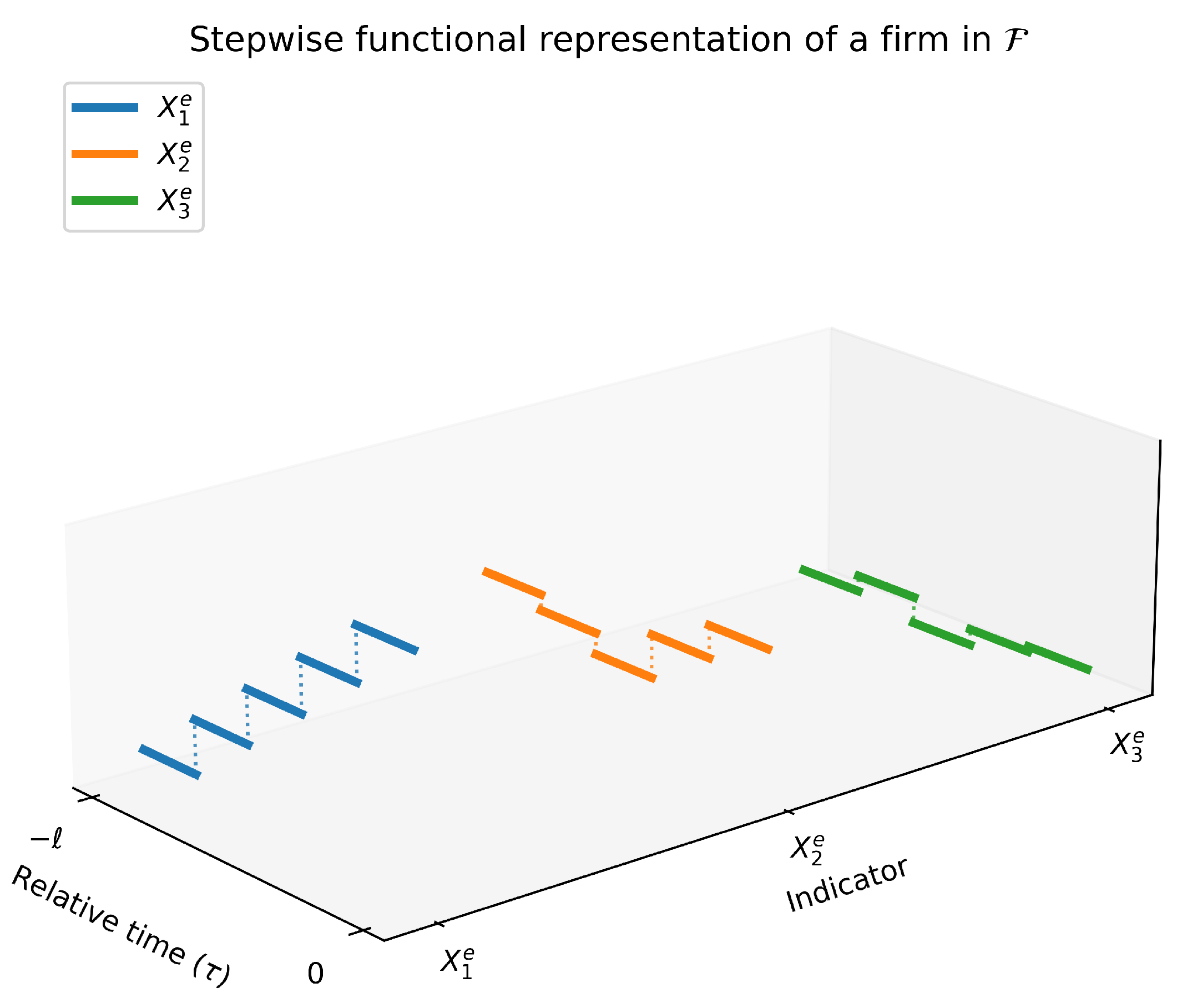
From a geometric perspective, each indicator can be interpreted as a stepwise function defined over the relative time domain, constant within each annual interval. Consequently, the firm is conceived as a discrete multivariate functional representation observed on a finite time grid, where financial dynamics are described through trajectories capturing the recent evolution of the indicators.

Figure 1 illustrates this interpretation for a hypothetical set of indicators.

2.6. Definition of a Functional Distance as a Semimetric

Once firms are represented as elements of $\mathcal{F}$ through multivariate financial trajectories over a fixed-length retrospective window ℓ, a dissimilarity measure is required to compare such trajectories coherently over time and across indicators. To this end, a composite functional distance is defined that (i) accumulates discrepancies over time, (ii) penalizes the loss of comparability when missing information is present, (iii) bounds the influence of extreme values, and (iv) preserves interpretability at the indicator level through a weighted combination. The proposed measure is formulated as a semimetric, in the sense that the triangle inequality is not required to hold, while fundamental properties such as non-negativity, identity of indiscernibles, and symmetry are preserved.

• Step 1: Accumulated Distance per Indicator

Consider the set of comparable time points for indicator j between two firms e and $e^{\prime }$, ${\mathcal{T}}_j^{e,e^{\prime }}\subseteq \{-\ell +1,\dots ,0\},$ defined as the time indices where both observations are available. The accumulated discrepancy per indicator is defined as

$$d_j^{\mathrm{acum}}(e,e^{\prime })=\sum _{t\in {\mathcal{T}}_j^{e,e^{\prime }}}\left|x_{j,t}^e-x_{j,t}^{e^{\prime }}\right|.$$

(3)

In this expression, the absolute value is naturally extended to $\overline{\mathbb{R}}$. In particular, the convention is adopted that $|+\infty -+\infty |=0$, while $|+\infty -a|=|a-+\infty |=+\infty$ for all $a\in \mathbb{R}$. This convention reflects the economic interpretation of financial indicators, in which infinite values typically arise from zero denominators. In this context, two matching infinite values reflect an equivalent structural condition, whereas the comparison between a finite value and an infinite one represents an extreme discrepancy in the corresponding indicator.

This summation accumulates the observed differences over time, capturing both the magnitude and the temporal persistence of the discrepancies between trajectories.

• Step 2: Domain-Loss Penalty

When $|{\mathcal{T}}_j^{e,e^{\prime }}|<\ell$, the comparison is performed over a subdomain and, therefore, a penalty proportional to the non-comparable fraction is incorporated. Define

$${\rho }_j(e,e^{\prime })=1-{\displaystyle \frac{|{\mathcal{T}}_j^{e,e^{\prime }}|}{\ell }},{\rho }_j(e,e^{\prime })\in [0,1].$$

(4)

Let $\lambda \ge 0$ be a penalty parameter. The penalized distance is given by

$$d_j^{\mathrm{pen}}(e,e^{\prime })=d_j^{\mathrm{acum}}(e,e^{\prime })\left(1+\lambda {\rho }_j(e,e^{\prime })\right).$$

(5)

This adjustment increases the distance when temporal comparability is lower, explicitly penalizing the lack of shared information between trajectories. Unlike imputation-based approaches, this mechanism does not introduce artificial values but instead reflects the uncertainty associated with incomplete comparisons.

• Step 3: bounding of extreme values.

To prevent extraordinary discrepancies from dominating the total distance, a bounded rational transformation is applied:

$${\tilde{d}}_j(e,e^{\prime })={\displaystyle \frac{d_j^{\mathrm{pen}}(e,e^{\prime })}{1+d_j^{\mathrm{pen}}(e,e^{\prime })}},{\tilde{d}}_j(e,e^{\prime })\in [0,1].$$

(6)

When $d_j^{\mathrm{pen}}(e,e^{\prime })=+\infty$, the expression converges to 1, ensuring that infinite discrepancies are bounded at the maximum possible value.

This transformation is increasing over $[0,+\infty ]$, preserves the relative ordering of discrepancies, and limits their maximum contribution per indicator. In this way, extreme values are prevented from dominating the global distance, ensuring a balanced contribution of each indicator in the comparison between trajectories.

• Step 4: optional incorporation of non-functional attributes.

Optionally, the dissimilarity measure can be extended to incorporate structural or contextual attributes that are not part of the temporal dynamics of financial trajectories.

Let $s_h(e,e^{\prime })\in [0,1]$ be a bounded distance function associated with attribute $h=1,\dots ,p$, defined according to the nature of the attribute (categorical, ordinal, spatial, or quantitative). These functions allow the comparison between firms to be complemented by incorporating additional relevant information, while maintaining scale comparability with the dynamic discrepancies and ensuring their coherent integration into the proposed semimetric.

This extension is useful in contexts where it is desirable to control for external factors or common conditions, such as aggregate shocks, sectoral differences, or institutional characteristics that are not directly reflected in financial trajectories.

However, in the empirical application developed in this study, the distance measure is constructed exclusively from financial trajectories, in order to isolate the contribution of the functional representation and ensure comparability with the benchmark models used in the empirical evaluation.

• Step 5: global weighted combination.

The total distance between two firms is defined as a convex combination of the considered components:

$$D(e,e^{\prime })=\sum _{j=1}^m{w}_j{\tilde{d}}_j(e,e^{\prime })+\sum _{h=1}^p{\alpha }_h{s}_h(e,e^{\prime }),$$

(7)

with

$$w_j\ge 0,{\alpha }_h\ge 0,\sum _{j=1}^m{w}_j+\sum _{h=1}^p{\alpha }_h=1.$$

In the baseline case considered in this study, the distance is constructed exclusively from the dynamic components ${\tilde{d}}_j$, that is, with $p=0$, which implies that ${\sum }_{j=1}^m{w}_j=1$.

The weights $w_j$ control the relative contribution of each financial indicator in the dissimilarity measure, introducing a degree of flexibility and interpretability to the model. In particular, this formulation allows the total distance to be decomposed into indicator-level contributions, facilitating the analysis of which financial dimensions explain the similarity between trajectories.

In the empirical implementation, this distance $D(e,e^{\prime })$ serves as the basis for the k-NN classifier, so that the selection of nearest neighbors is performed in the functional space defined by the proposed semimetric.

The function $D(·,·)$, defined as a combination of the functional discrepancies (and, optionally, non-functional attributes), constitutes a semimetric. In particular, it is not required to satisfy all classical metric properties, such as the triangle inequality.

The violation of the triangle inequality arises from the functional component, due to the domain-loss penalty and the comparison over shared time domains. This behavior is consistent with the use of semimetrics in functional classification contexts, where the distance function is defined based on practical criteria for comparing trajectories rather than on strict adherence to metric properties (Ferraty & Vieu, 2003; James et al., 2023).

Nevertheless, the construction preserves fundamental properties such as non-negativity, symmetry, and the identity of indiscernibles, and is fully suitable for the central objective of the study: comparing firms based on the overall similarity of their financial trajectories. In particular, this formulation preserves interpretability and explicit control over each source of discrepancy, while providing a coherent basis for the application of the k-NN classifier in the defined functional space.

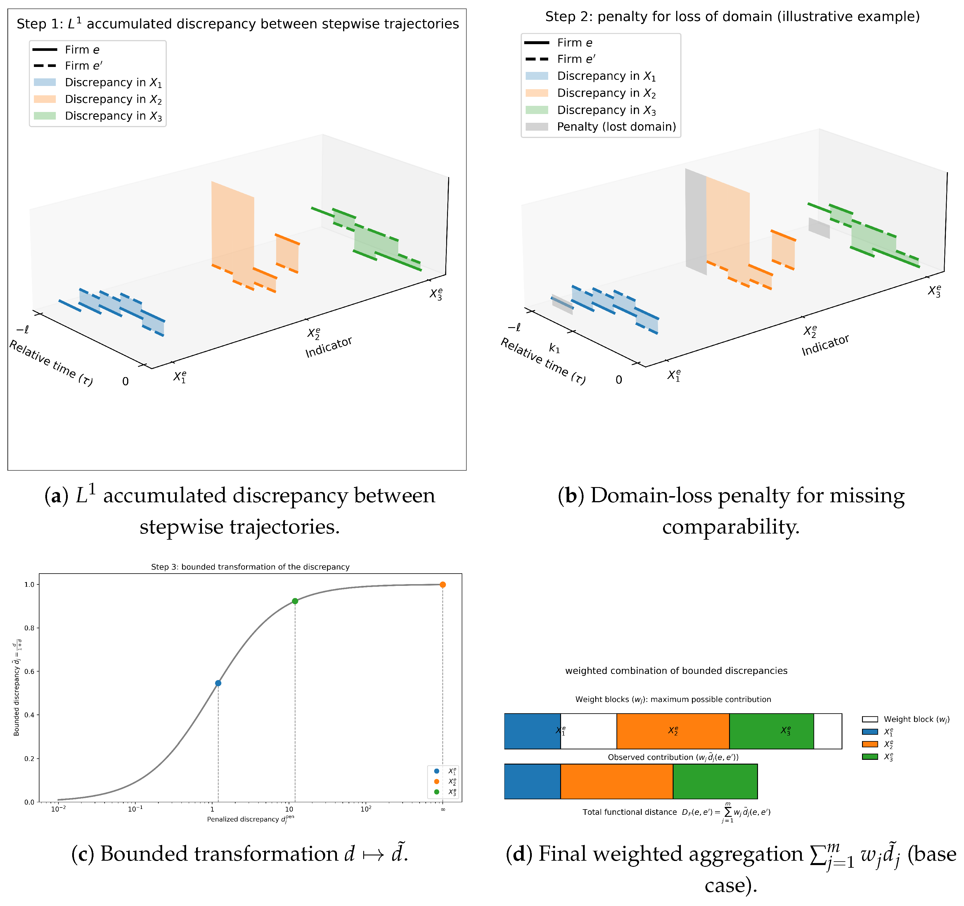
Figure 2 summarizes the step-by-step construction of the proposed functional distance, highlighting: (a) $L^1$ accumulated discrepancy, (b) domain-loss penalty, (c) bounded transformation, and (d) final weighted aggregation.

2.7. Functional k-NN Classifier Based on the Proposed Metric

Once the functional representation of financial trajectories and the similarity metric between firms have been defined, the classification stage is implemented using a k-nearest neighbors (k-NN) classifier. In this approach, the k-NN algorithm does not constitute the central methodological contribution of the study, but rather serves as a transparent mechanism to leverage the proposed composite distance and to structure comparisons between firms based on their recent financial evolution.

Formally, for a target firm e, its k nearest neighbors are identified as those that minimize the total distance $D(e,e^{\prime })$ defined in the previous section. Let $\mathcal{E}$ denote the set of firms available in the sample. The neighborhood is defined as

$${\mathcal{N}}_k\left(e\right)=\left\{e^{\prime }\in \mathcal{E}\backslash \left\{e\right\}:D(e,e^{\prime })\mathrm{is}\mathrm{among}\mathrm{the}k\mathrm{smallest}\mathrm{values}\right\}.$$

The resulting neighborhood ${\mathcal{N}}_k\left(e\right)$ consists of firms whose multivariate financial trajectories exhibit patterns similar to those of the target firm, according to the previously defined accumulated, penalized, bounded, and weighted distance.

The estimation of the risk associated with condition $RQ$ is obtained by aggregating the observed states of the selected neighbors. In this implementation, a uniform voting scheme is used, defining the empirical score as the proportion of firms classified as $RQ=1$ within the neighborhood:

$$\widehat{p}\left(e\right)={\displaystyle \frac{1}{k}}\sum _{e^{\prime }\in {\mathcal{N}}_k\left(e\right)}{y}_{e^{\prime }},$$

where $y_{e^{\prime }}\in \{0,1\}$ denotes the observed state of the variable $RQ$ for the neighboring firm $e^{\prime }$. This value can be interpreted as an empirical measure of relative risk based on observed precedents in firms with similar financial trajectories, rather than as a structural probability of bankruptcy.

This nonparametric approach allows the estimation of risk from similarity patterns in the observed data, without imposing specific functional assumptions on the relationship between financial indicators and the risk condition.

In addition to the point estimate, the procedure explicitly identifies the set of nearest firms in the trajectory space $\mathcal{F}$, facilitating the comparative analysis of financial dynamics and observed outcomes within each neighborhood, thereby reinforcing the interpretability of the model.

2.8. Hyperparameter Optimization and Model Calibration

The functional k-NN classifier and the proposed distance depend on a set of hyperparameters that were calibrated empirically. In particular, the following were considered: (i) the length of the retrospective window ℓ, (ii) the number of neighbors k, (iii) the penalty parameter $\lambda$ for temporal domain loss in the functional component, and (iv) the weights associated with the financial indicators ($w_j$), subject to non-negativity and unit-sum constraints.

In a preliminary stage, different values of the retrospective window length $\ell \in \{3,4,5,6,7\}$ were evaluated using stratified cross-validation, with the average F1-score as the comparison criterion. Based on this analysis, $\ell =5$ was selected as the final configuration, as it provides an appropriate balance between discriminatory power and information availability.

Once the window length was fixed, the calibration of k and $\lambda$ was carried out using Bayesian optimization implemented with Optuna (TPE sampler) (Akiba et al., 2019), maximizing the average F1-score under internal stratified 5-fold cross-validation. To assess the stability of the optimization process, independent runs were performed using different random seeds, a 10% subsample of the firms, and 30 trials in each case.

The use of subsamples is motivated by computational cost considerations, as repeated evaluation of the functional k-NN classifier involves computing distances over full trajectories. Nevertheless, the consistency of the results obtained across multiple runs supports the stability of the identified optimal configuration.

Based on this analysis, the final configuration of k and $\lambda$ was estimated through a refined search on an expanded subsample of 20% and a larger number of evaluations (50 trials), maintaining the same internal cross-validation scheme.

Subsequently, once the optimal values of k and $\lambda$ were fixed, the weights associated with the 17 financial indicators were estimated using an analogous optimization scheme with Optuna, again maximizing the F1-score under internal stratified 5-fold cross-validation. Similarly, the stability of the weights was assessed through independent runs with different seeds, and the final configuration was obtained from a refined search with a larger subsample size and a higher number of evaluations.

For this stage, Optuna optimized raw weights $v_j\in [0.1,5.0]$ for each indicator, which were subsequently normalized to satisfy the convex combination constraint:

$$w_j={\displaystyle \frac{v_j}{{\sum }_q{v}_q}},$$

ensuring that all weights are non-negative and sum to one. In this way, the calibration preserves flexibility in the relative importance of each indicator while maintaining the interpretability of the functional distance.

Although a nested cross-validation scheme could provide a more exhaustive evaluation of the hyperparameter selection process, the adopted strategy strikes a balance between computational feasibility and empirical robustness, supported by the stability analyses performed.

2.9. Model Evaluation Strategy

Once the optimal configuration of the model was fixed, model performance was evaluated on the full sample using stratified 10-fold cross-validation, preserving the proportion of firms classified as $RQ=1$ in each fold. Stratification and partitioning were performed at the firm level (NIT), so that all observations associated with the same firm (i.e., its entire trajectory) remained within the same fold, thereby avoiding information leakage between the training and test sets.

This evaluation stage was carried out completely independently of the hyperparameter optimization process. In particular, the values of ℓ, k, $\lambda$, and the weights $w_j$ were fixed in advance and were not recalibrated during the final cross-validation.

The evaluation metrics considered include Accuracy, Precision, Recall, F1-score, Matthews Correlation Coefficient (MCC), Area Under the ROC Curve (AUC-ROC), Average Precision, and Log-loss. Given the binary classification setting and the interpretation of the dependent variable as a proxy for financial distress, the F1-score was adopted as the primary evaluation metric, while MCC and Average Precision were used as complementary measures that are particularly informative in this context.

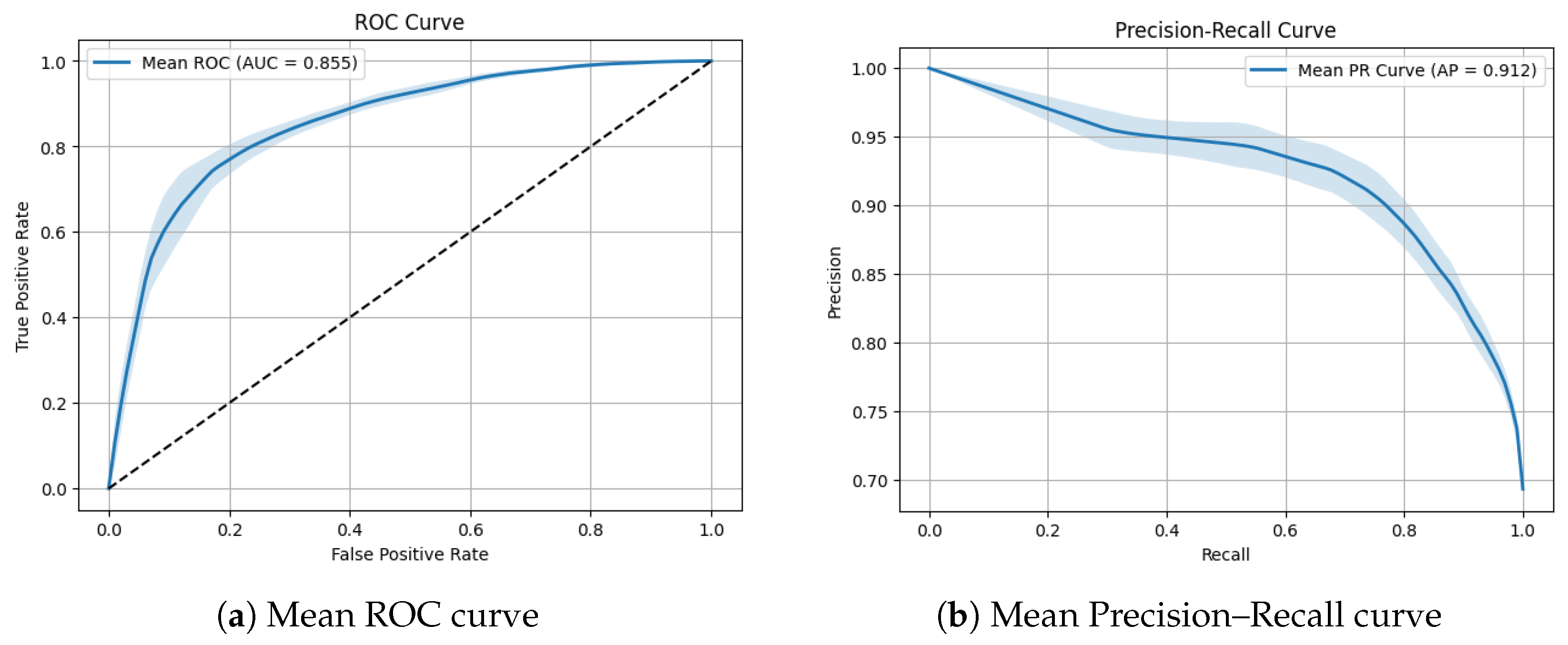
For each partition, ROC and Precision–Recall curves were also obtained, from which average curves were constructed by interpolation over a common grid. The mean and standard deviation of the metrics across folds are reported to assess the stability of the model under different sample partitions.

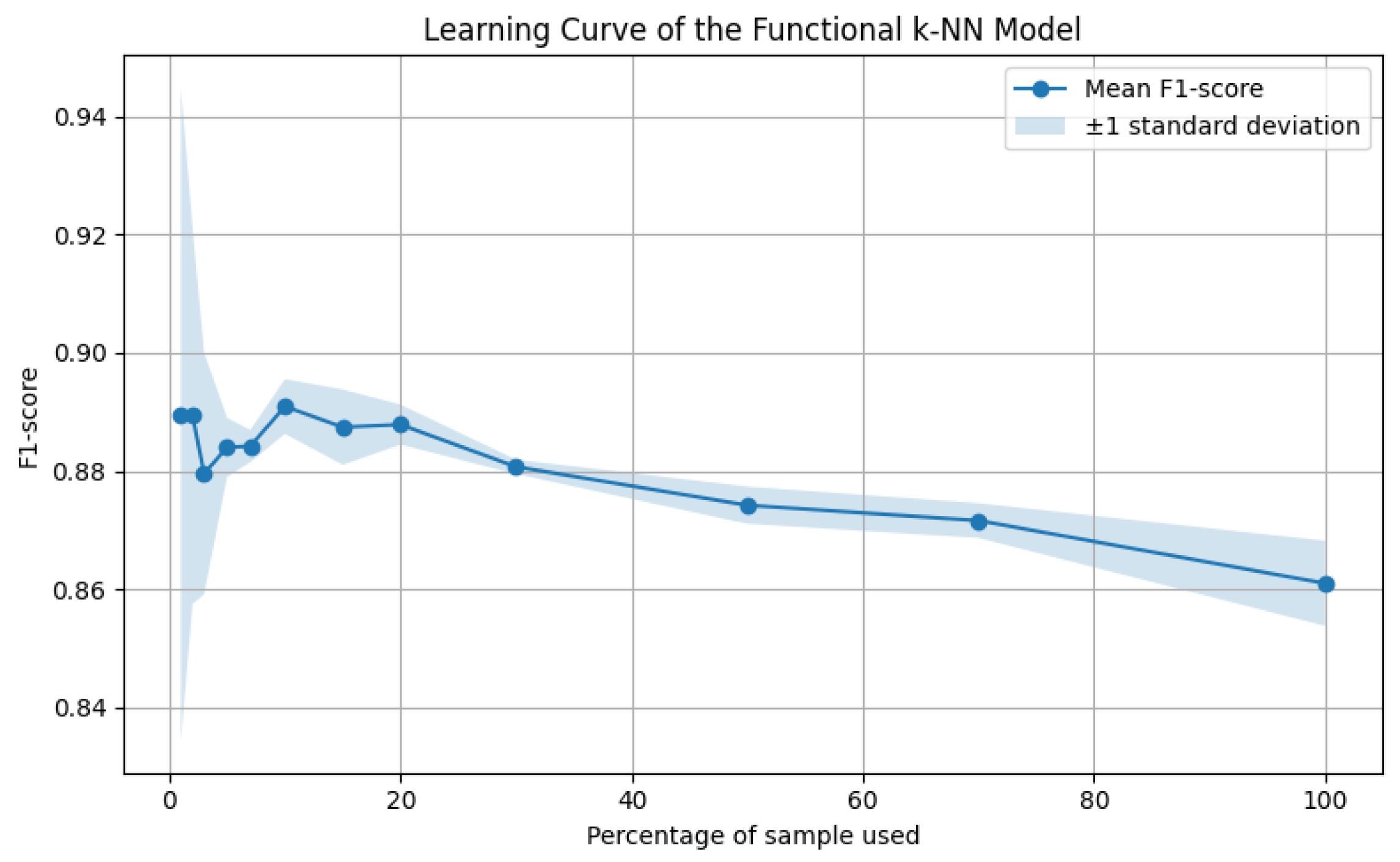
Finally, the robustness of the model was examined through two complementary exercises: a learning curve constructed using increasing proportions of the full sample, and a bootstrap resampling procedure, to assess the sensitivity of performance to sample size and variations in sample composition.

Although a nested cross-validation scheme could provide a more conservative estimate of performance, the adopted strategy explicitly separates the calibration stage from the final evaluation stage and is complemented by stability analyses, yielding a robust and computationally feasible assessment of the model.

3. Results

This section presents the empirical results obtained from the implementation of the functional k-NN model, including its calibration, discriminative performance, and stability analysis.

3.1. Sample Description and Functional Representation

The final sample consists of 5565 firms from the tourism sector in Colombia with complete financial trajectories over a five-year retrospective window. For each firm, 17 selected financial indicators were used, from which the multivariate functional representation employed in the classification process was constructed.

In this sample, 69.36% of the trajectories are classified as $RQ=1$, while 30.64% correspond to $RQ=0$. As explained in the methodological section, this distribution reflects the way in which the dependent variable is constructed, integrating both the exit of firms from the reporting system and their persistence in administrative states associated with financial difficulties. Therefore, this proportion should not be interpreted as a population bankruptcy rate, but rather as a feature of the study design.

In this sense, the model results should be interpreted in the context of a financial trajectory classification problem in relative time, rather than as an estimation of bankruptcy probability in a population setting. Consequently, the performance metrics reflect the model’s ability to discriminate patterns of financial distress within this specific design, rather than its behavior in a traditional firm–year prediction context.

To complement the characterization of the dependent variable,

Table 3. Sample distribution according to the category observed in the final year of the trajectory.

Category	Frequency	Percentage
Reporting discontinuity	3738	67.17
Active	1701	30.56
Pre-operational stage	3	0.05
Restructuring agreement	20	0.36
Reorganization agreement	103	1.85
Total	5565	100.00

presents the distribution of the sample according to the category observed in the final year of each trajectory.

The largest proportion of trajectories corresponds to firms that do not reach the last year of the study horizon, representing 67.17% of the sample. To a lesser extent, there are firms that remain active or in a pre-operational stage, as well as those in administrative states associated with reorganization or restructuring processes.

This pattern is consistent with the way financial trajectories are constructed in the model, which are defined in relative time and anchored at the last observed year of each firm. Consequently, a substantial fraction of trajectories corresponds to firms that stop reporting information during the analysis period, without this necessarily implying an observed bankruptcy event.

3.2. Hyperparameter Optimization

Model calibration was conducted by evaluating different retrospective window lengths $\ell \in \{3,4,5,6,7\}$ years. For each value of ℓ, the full optimization and validation procedure was executed, showing that $\ell =5$ provided the best balance between discriminative performance and stability. This value was therefore selected for the final analysis.

With the temporal window defined, the optimization of the hyperparameters k and $\lambda$ was carried out using Bayesian search implemented with Optuna, maximizing the average F1-score under internal stratified cross-validation.

To assess the stability of the optimization process, 10 independent runs were performed using different random seeds, a 10% subsample of the data, and 30 trials in each case. The results show that the optimal values of k were concentrated in the range $[11,15]$, while the parameter $\lambda$ had a mean of 4.04 and a standard deviation of 0.60. The F1-score, in turn, reached a mean of 0.896 with a standard deviation of 0.013, indicating low variability in model performance across runs.

These results indicate that the optimization process is stable with respect to changes in the random seed and the subsample used.

It is important to note that these values correspond to the performance observed during the optimization phase under internal cross-validation and on subsamples of the dataset. Therefore, they are not directly comparable to the final evaluation results reported in the following section, which are obtained on the full sample under an independent cross-validation scheme.

Based on this analysis, the final model configuration was estimated using an expanded subsample of 20% and 50 trials in order to refine the hyperparameter estimates. At this stage, the optimal values obtained were $k=15$ and $\lambda =4.1305$, with an average F1-score of 0.8741 during internal validation.

Subsequently, keeping the optimal values of k and $\lambda$ fixed, the weights associated with the 17 financial indicators were estimated using an analogous optimization scheme based on Optuna, maximizing the F1-score under internal stratified cross-validation.

To assess the stability of the estimated weights, 10 independent runs were performed using different random seeds, a 10% subsample of the data, and 30 trials in each case. The weights obtained were normalized in each run to ensure their comparability.

Table 4. Stability of the estimated weights for the main financial indicators.

Indicator	Mean	Std. Dev.
RCC	0.1055	0.0268
AFT	0.0747	0.0351
RCID	0.0695	0.0316
RCP	0.0681	0.0235
PPI	0.0590	0.0389
RA	0.0589	0.0372
MO	0.0575	0.0313
RI	0.0554	0.0434
ROE	0.0551	0.0307
PPP	0.0551	0.0396

presents a summary of the results obtained, reporting the mean and standard deviation of the weights for the main indicators. It is observed that, although there is some variability in the estimated values, the indicators with the highest weights remain consistent across runs.

These results show that, although the specific values of the weights exhibit moderate variation, the relative importance structure across indicators remains stable. In particular, variables such as RCC, AFT, and RCID consistently appear among those with the highest contributions, suggesting that the model identifies robust patterns of financial similarity across trajectories.

Table 5. Final normalized weights of the functional k-NN model.

Indicator	Weight
AFT	0.0900
PPI	0.0881
RAO	0.0858
RCID	0.0812
RCC	0.0807
MO	0.0770
ROE	0.0742
RA	0.0672
RI	0.0646
LG	0.0625

presents the final normalized weights obtained in the model estimation. It is observed that the indicators AFT, PPI, and RAO account for the largest contributions to the functional metric, followed by RCID and RCC.

This distribution is consistent with the stability analysis presented previously, in which these same indicators appear recurrently among those with the highest importance. Overall, these results indicate that the proposed functional metric assigns greater relevance to variables associated with activity and operating profitability, reinforcing the model’s ability to capture meaningful financial patterns in trajectory comparisons.

Likewise, the consistency between the stability results and the final configuration suggests that the optimization process is able to identify robust structures in the measurement of similarity between firms, strengthening both the methodological validity and the interpretability of the functional k-NN model.

3.3. Model Performance

Once the optimal configuration of the model was fixed, its performance was evaluated using stratified 10-fold cross-validation. The evaluation was conducted using the previously computed functional distance matrix, without performing additional recalibration during this stage.

The average results obtained under this validation scheme are presented in

Table 6. Performance of the functional k-NN model under stratified 10-fold cross-validation.

Metric	Mean	Std. Dev.
Accuracy	0.7899	0.0097
Precision	0.7955	0.0073
Recall	0.9386	0.0171
F1-score	0.8610	0.0072
MCC	0.4700	0.0267
AUC	0.8555	0.0163
Average Precision	0.9117	0.0111
Log-loss	0.7771	0.1236

. Unlike the values reported during the optimization phase, these metrics correspond to the final evaluation of the model on the full sample. Given the imbalance in the dependent variable, a set of complementary metrics is reported to assess the model’s discriminative ability from different perspectives.

The model achieves an average F1-score of 0.8610 (±0.0072), along with a recall of 0.9386 and a precision of 0.7955. These results indicate that the model identifies a high proportion of trajectories classified as $RQ=1$, while maintaining a moderate level of false positives. The average accuracy is 0.7899.

From an overall classification perspective, the Matthews Correlation Coefficient (MCC) reaches a value of 0.4700 (±0.0267), reflecting consistent performance when considering both correct and incorrect classifications across classes. In terms of discriminative ability, the model presents an AUC of 0.8555 (±0.0163).

In the Precision–Recall space, the Average Precision reaches a value of 0.9117 (±0.0111), which is consistent with the expected behavior in imbalanced classification settings. Finally, the average log-loss is 0.7771.

The low standard deviations across all metrics indicate high model stability across the different cross-validation folds, suggesting that its performance is robust to variations in sample composition.

ROC and Precision–Recall Analysis

The average ROC and Precision–Recall curves obtained from stratified 10-fold cross-validation are presented in Figure 3. Both curves exhibit stable behavior across the different folds, which is consistent with the stability observed in the reported metrics.

The ROC curve reflects an adequate overall discriminative ability, consistent with the AUC value of 0.8555 reported in Table 6. This indicates that the model consistently separates trajectories classified as $RQ=1$ from those classified as $RQ=0$ across different decision thresholds.

In turn, the Precision–Recall curve shows a stable balance between precision and recall across different thresholds. Given the class imbalance in the dependent variable, this curve provides complementary evidence of the model’s ability to identify trajectories associated with $RQ=1$ while maintaining a controlled level of false positives.

3.4. Robustness Analysis

To evaluate the stability of the model under different sampling conditions, two complementary exercises were conducted: (i) learning curve analysis and (ii) a bootstrap procedure.

The learning curve was constructed using increasing proportions of the full sample, while keeping the model configuration fixed. The results are presented in Figure 4. It is observed that the F1-score progressively converges toward the value obtained using 100% of the data ($0.8610\pm 0.0072$), suggesting stable performance and the absence of significant dependence on sample size.

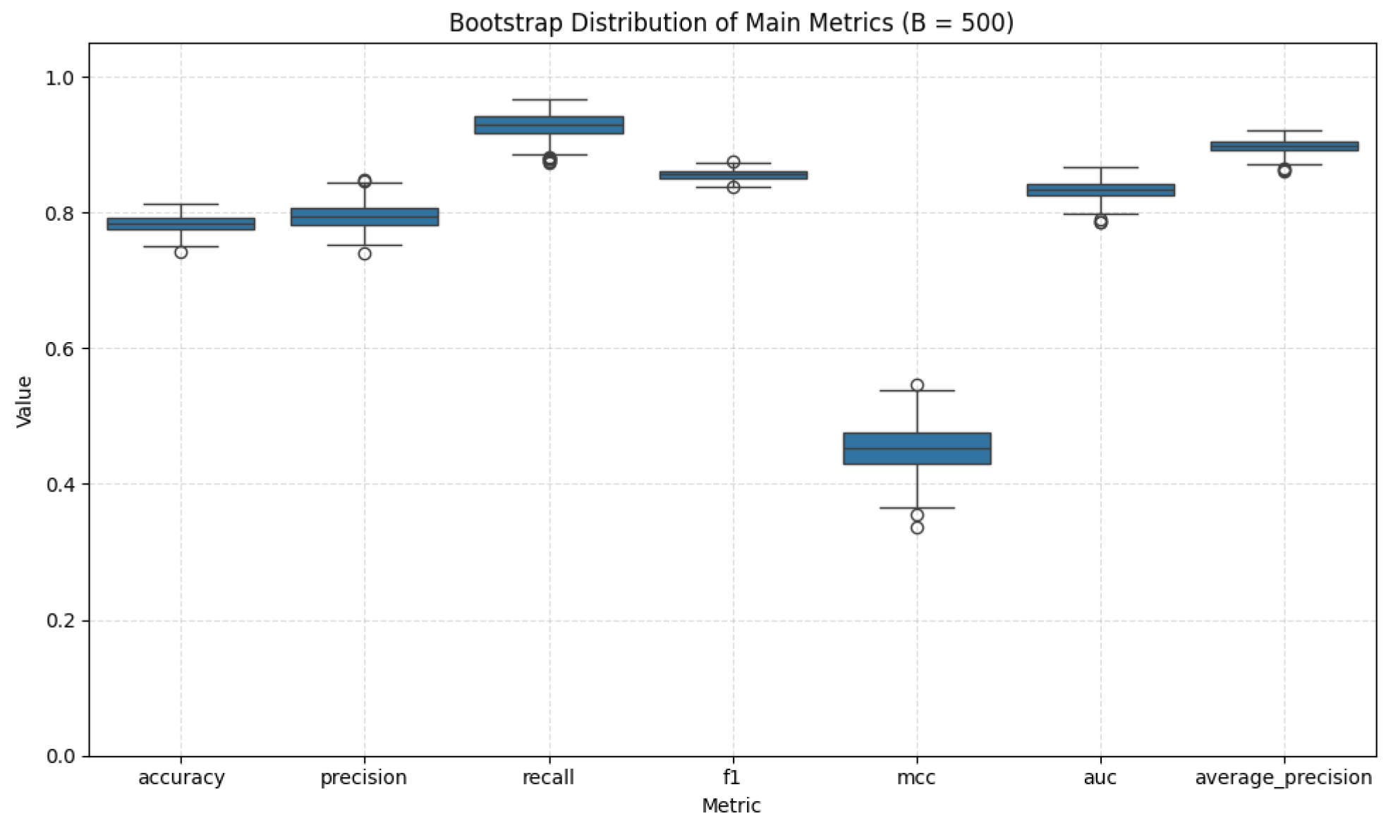
Additionally, a bootstrap procedure with 500 replications was applied to evaluate the stability of the metrics under resampling. For each metric, 95% percentile confidence intervals were computed. The results are presented in

Table 7. Bootstrap performance results (500 replications) with 95% confidence intervals.

Metric	Mean	Std. Deviation	95% CI
Accuracy	0.7839	0.0119	[0.7595, 0.8062]
Precision	0.7949	0.0185	[0.7622, 0.8307]
Recall	0.9289	0.0174	[0.8923, 0.9586]
F1-score	0.8564	0.0068	[0.8426, 0.8696]
MCC	0.4539	0.0339	[0.3826, 0.5204]
AUC	0.8342	0.0131	[0.8085, 0.8571]
Average Precision	0.8983	0.0100	[0.8766, 0.9144]
Log-loss	1.0441	0.1418	[0.8038, 1.3498]

.

Figure 5 presents the distribution of the main metrics obtained through the bootstrap procedure. It is observed that, although some dispersion exists—particularly in metrics such as MCC—the distributions remain concentrated within ranges consistent with the cross-validation results.

Overall, the learning curve indicates stability with respect to sample size, while the bootstrap procedure shows consistency under resampling. These results support the robustness of the functional k-NN model under different sample configurations.

3.5. Interpretability of the Functional Metric

One of the central contributions of the proposed approach is its interpretability, in the sense that the functional metric allows the explicit identification of the relative contribution of each financial indicator in the computation of similarity between firms. In particular, the estimated weights determine the importance of each dimension in the final distance used by the classifier.

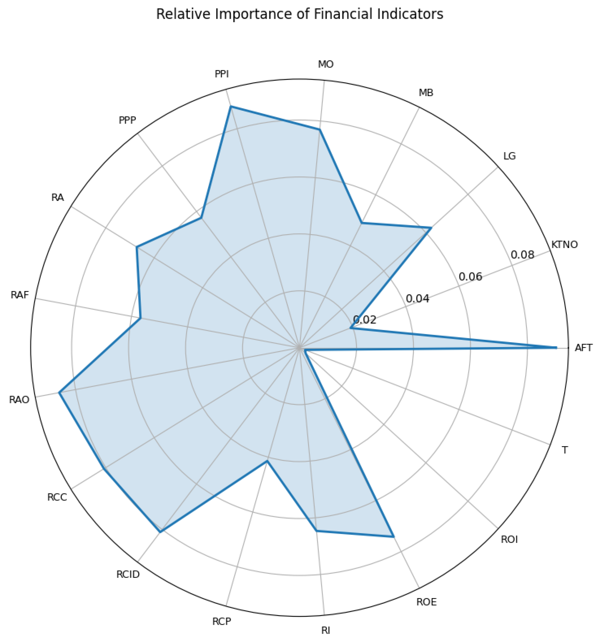
Figure 6 presents the relative structure of the normalized weights for the 17 financial indicators considered in the model. This representation provides a compact visualization of the distribution of importance across indicators and facilitates the traceability of the classification process.

It is observed that variables such as AFT, PPI, and RAO concentrate the highest weights, indicating that differences in these indicators have a predominant influence on the identification of similar financial trajectories. In contrast, other indicators exhibit more moderate contributions, reflecting a lower influence on the structure of the functional distance.

Overall, these results show that the model not only discriminates trajectories based on their financial similarity, but also provides an explicit decomposition of such similarity in terms of specific indicators. This facilitates the interpretation of proximity patterns between firms and reinforces the traceability of the classification process in the functional space.

3.6. Comparison with Baseline Models

To evaluate the performance of the proposed model in a comparative setting, several baseline models commonly used in the bankruptcy prediction literature were estimated, including logistic regression, k-NN with static variables, Random Forest, and XGBoost. All models were evaluated using the same dataset, the same financial trajectory structure constructed through five-year retrospective windows, and the same stratified 10-fold cross-validation scheme, ensuring the comparability of the results.

It is important to note that, in all cases, the variables used correspond exclusively to the information contained in the financial trajectories, in order to isolate the contribution of the proposed functional metric.

The comparative results are presented in

Table 8. Comparative performance of baseline models under stratified 10-fold cross-validation.

Model	Acc.	Prec.	Rec.	F1	MCC	AUC	AP	LogLoss
Logistic Regression	0.6931	0.7013	0.9712	0.8145	0.0806	0.6676	0.7960	0.7273
k-NN Static	0.7384	0.7748	0.8780	0.8231	0.3381	0.7516	0.8495	0.6646
Random Forest	0.8924	0.9051	0.9438	0.9240	0.7418	0.9550	0.9787	0.2659
XGBoost	0.9066	0.9275	0.9389	0.9331	0.7789	0.9629	0.9837	0.2273
k-NN (proposed)	0.7899	0.7955	0.9386	0.8610	0.4700	0.8555	0.9117	0.7771

.

The comparison between the traditional k-NN and the proposed functional k-NN model allows the contribution of the distance metric to be clearly identified. Although both approaches are based on similarity-based classification schemes, the proposed model exhibits consistent improvements across all considered metrics.

In particular, the F1-score increases from 0.8231 to 0.8610. Although this difference is moderate, a more pronounced improvement is observed in metrics that more comprehensively capture performance in imbalanced settings, such as the Matthews Correlation Coefficient (from 0.3381 to 0.4700). Additionally, relevant increases are observed in terms of AUC (from 0.7516 to 0.8555) and Average Precision (from 0.8495 to 0.9117), indicating a better capacity for discrimination and ranking of trajectories according to the $RQ$ condition.

Overall, these results suggest that the proposed functional metric more effectively captures the dynamic structure of financial trajectories, improving both classification performance and ranking quality compared to k-NN based on static variables.

In comparison with tree-based models such as Random Forest and XGBoost, the proposed model exhibits lower performance in terms of classification metrics. However, these models are designed to maximize predictive performance in high-complexity spaces, whereas the proposed functional approach prioritizes interpretability and traceability of the classification process.

In this sense, the functional k-NN model is positioned as a complementary alternative, oriented toward contexts where it is relevant not only to discriminate trajectories, but also to understand the financial dimensions that explain such similarity. In particular, the ability to explicitly identify comparable firms and to decompose the distance into indicator-level contributions constitutes a methodological advantage over more opaque approaches.

3.7. Illustrative Case Study

To illustrate the interpretability of the proposed functional k-NN model, a representative firm classified with a high probability associated with the condition $RQ=1$ is analyzed. The estimated score is constructed from the proportion of firms classified as $RQ=1$ within its $k=15$ nearest neighbors.

In this case, the target firm presents a value of $\widehat{p}\left(e\right)=0.93$. This result is consistent with the composition of its neighborhood, in which 14 out of the 15 neighbors correspond to firms with $RQ=1$, indicating that the firm is located in a region of the functional space associated with trajectories similar to those classified as experiencing financial distress.

Table 9. Nearest neighbors of the target firm.

Neighbor (Idx_Base)	RQ	Distance
3380	1	0.6446
3682	1	0.6395
380	1	0.6304

presents the nearest neighbors of the target firm, identified by their index in the dataset and their functional distance.

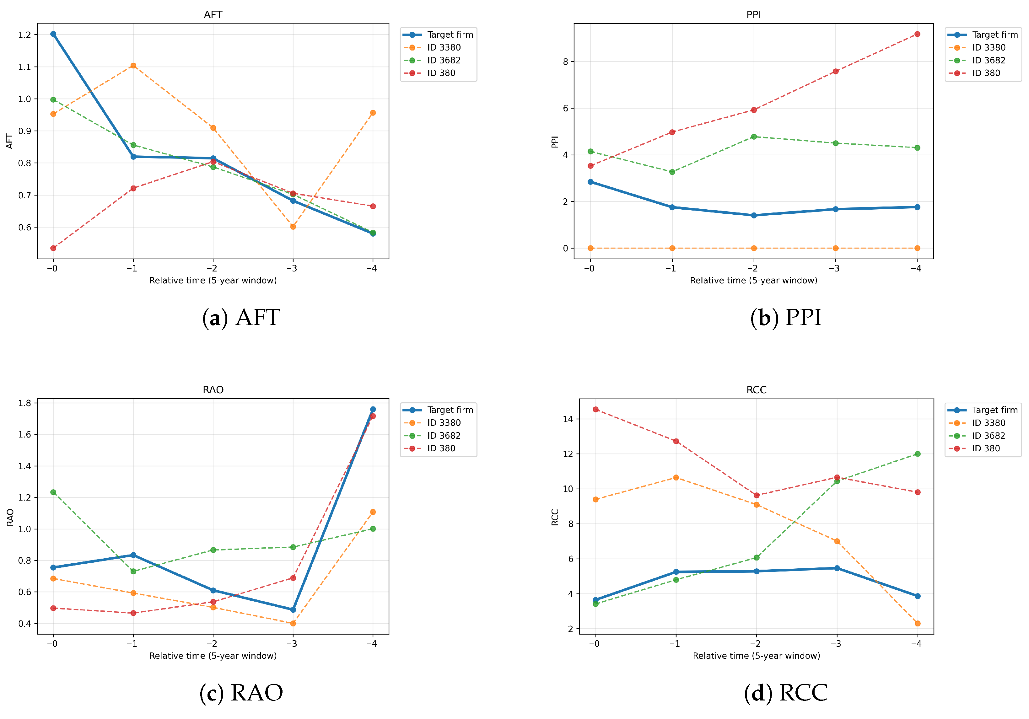
The model not only identifies nearest neighbors, but also allows the observation of how similarities manifest in the trajectories of the most relevant indicators. Figure 7 shows the evolution of the target firm and its neighbors across the indicators with the highest weights in the functional metric.

The similarity between the target firm and its neighbors is explained by the shape and evolution of their trajectories in the most relevant indicators. In AFT, for example, the target firm exhibits a downward trend over the period, accompanied by trajectories of its neighbors that follow comparable patterns in terms of level and variation.

In RAO and RCC, similar behaviors are also observed in the temporal dynamics, with changes in the most recent periods that, although not identical, are sufficiently close in shape to be considered proximate under the functional metric. In the case of PPI, although there are differences in levels across firms, the trajectories remain within comparable ranges, which does not generate significant separation in terms of distance.

Overall, these patterns show that proximity between firms does not depend on pointwise coincidences, but rather on comparable dynamic structures over time. In this way, the target firm is located within a neighborhood composed mainly of trajectories classified as $RQ=1$, which explains the high score assigned by the model. Moreover, the proposed approach makes it possible to identify the specific dimensions in which such similarity is constructed, providing a clear and traceable interpretation of the classification process.

4. Discussion

The results show that the proposed functional approach improves the performance of the k-nearest neighbors classifier in identifying financial trajectories associated with conditions of corporate risk. In the bankruptcy prediction literature based on firm–year observations and static variables, the conventional k-NN algorithm typically does not stand out compared with more complex methods (Zhao et al., 2024). In this study, the same objective—the identification of firms at risk—is addressed through a different formulation, in which firms are represented by multivariate financial trajectories constructed from retrospective windows, and classification is performed based on a similarity measure consistent with this representation. In this sense, the results suggest that classification performance does not depend solely on the algorithm, but on the integrated system that combines temporal representation, the definition of the target variable, and the distance metric between trajectories.

A key element for interpreting these results lies in the way the target variable $RQ$ is defined. Unlike traditional approaches in the literature, $RQ$ does not correspond to a single event of legal bankruptcy, but rather to a construction that combines reporting discontinuity and administrative states associated with financial distress. Consequently, the positive class includes both firms that exit the reporting system and those that remain under formal conditions of deterioration.

This definition, together with the use of retrospective trajectories anchored to the last observed year, conditions the way in which the results should be interpreted. In particular, the proportion of firms classified as being at risk within the sample should not be understood as a population bankruptcy rate, but rather as a consequence of the representation design and the trajectory selection criteria. Under this approach, the objective is to discriminate patterns of financial evolution associated with conditions of deterioration or stability, rather than to predict a single event in a population-representative setting.

In this context, the representation based on retrospective windows allows capturing the recent evolution of financial indicators, recognizing that deterioration processes tend to develop gradually. For this reason, the analysis of multivariate trajectories is more informative than the use of isolated firm–year observations, as it allows identifying complete patterns of financial evolution rather than point-in-time states.

The comparison between these trajectories is performed using the proposed functional metric, which is integrated with the way trajectories are constructed and the target variable is defined to establish similarity between firms in the functional space. This distance evaluates similarity by considering both the magnitude and persistence of differences over time and incorporates weights that reflect the relative importance of each financial indicator. In this way, the similarity measure captures dynamic structures in firm evolution beyond pointwise discrepancies.

It should be noted that trajectories are constructed in relative time, anchored to the last year with available information for each firm, rather than being aligned by calendar year. This decision allows the comparison of financial evolution processes, prioritizing the identification of dynamic patterns over temporal synchronization across firms. However, this approach implies a trade-off: it improves comparability in the internal evolution of trajectories at the cost of not explicitly controlling for common macroeconomic conditions within the same period.

Within this same framework, a possible extension would be to incorporate contextual variables or macroeconomic factors into the distance computation through non-functional attributes. However, in the empirical application developed in this study, the comparison is conducted exclusively based on financial information, in order to isolate the contribution of the functional representation and the metric to model performance.

In addition to its performance, the approach presents a relevant advantage in terms of interpretability (Carmona et al., 2022). This does not arise solely from the use of the k-NN classifier, but from the integration between the functional representation and the distance metric. In particular, the metric allows the decomposition of similarity between firms in terms of each indicator and its evolution over time, incorporating weights that reflect their relative importance.

As a result, the model not only produces a score based on the proportion of neighbors in a risk condition, but also allows for the explicit analysis of the comparable trajectories that support such classification. This facilitates the traceability of the result and the understanding of the financial dynamics associated with patterns of deterioration or stability.

Another relevant aspect is the observed stability of performance. Cross-validation shows that classification ability remains consistent across different sample partitions, suggesting that the results do not depend on a particular data configuration. This stability is consistent with the structure of the approach, in which the combination of fixed-length trajectories and a metric designed to capture persistent patterns allows identifying regularities in firms’ financial evolution.

The proposed approach can also be situated relative to more complex machine learning models used in corporate risk analysis (Dasilas & Rigani, 2024; Zhao et al., 2024). While such models often achieve high predictive performance, their internal functioning may be difficult to interpret. In contrast, the functional approach introduces a different perspective by working with multivariate financial trajectories and incorporating a dynamic dimension into firm comparison.

In this way, the model operates not only as a classification mechanism, but also as a tool for analyzing similarities between trajectories in a transparent manner. In practical applications, it can complement more complex models by enabling explicit identification of comparable firms and the analysis of the dynamics that explain their proximity.

Finally, although this study focuses on the classification of financial trajectories associated with corporate risk conditions, the approach can be extended to other contexts where it is relevant to compare multivariate dynamics over time. In general terms, the contribution of the approach lies in the coherent integration of a trajectory-based representation, a functional metric designed to capture dynamic similarity, and an interpretable classification scheme, providing a transparent methodological framework for analyzing firm evolution.

5. Conclusions

This study proposes a functional approach for the classification of financial trajectories associated with corporate risk conditions, based on the representation of firms through multivariate trajectories and the use of a k-nearest neighbors classifier. Unlike traditional approaches based on isolated firm–year observations, the developed framework models each firm based on the recent evolution of its financial indicators through retrospective windows, allowing the capture of gradual patterns of deterioration or stability over time.

The central contribution of the study lies in the coherent integration of a trajectory-based representation, a similarity measure consistent with this representation, and an interpretable classification scheme. This integration allows firms to be compared based on their temporal evolution rather than on point-in-time states, facilitating the identification of financial patterns associated with risk conditions.

Through this structure, the model not only produces a risk score based on the proportion of neighbors under similar conditions, but also enables the identification of historically comparable firms whose trajectories can be directly analyzed. This feature introduces an interpretative component that facilitates the traceability of the results and the analysis of the financial dynamics associated with each classification.

In comparison with more complex machine learning models, which often achieve high levels of performance at the cost of lower interpretability, the proposed approach offers a transparent methodological framework that allows classification to be complemented with a structured analysis of similarities between firms. In this sense, the model is not intended to replace such approaches, but rather to provide a complementary perspective based on the comparison of financial trajectories.

Finally, the functional framework developed can be extended to other contexts in which it is relevant to compare multivariate dynamics over time, such as firm performance analysis, financial distress processes, or sectoral studies based on longitudinal data. Overall, the study provides a systematic and transparent way to analyze the financial evolution of firms based on their trajectories.