4.1. H1: Systematic Risk Assessment: Beta Factor Analyses
Beta factor distributions are analyzed using multiple visualization techniques by distributional parameters, including means, medians, and 95% confidence intervals.
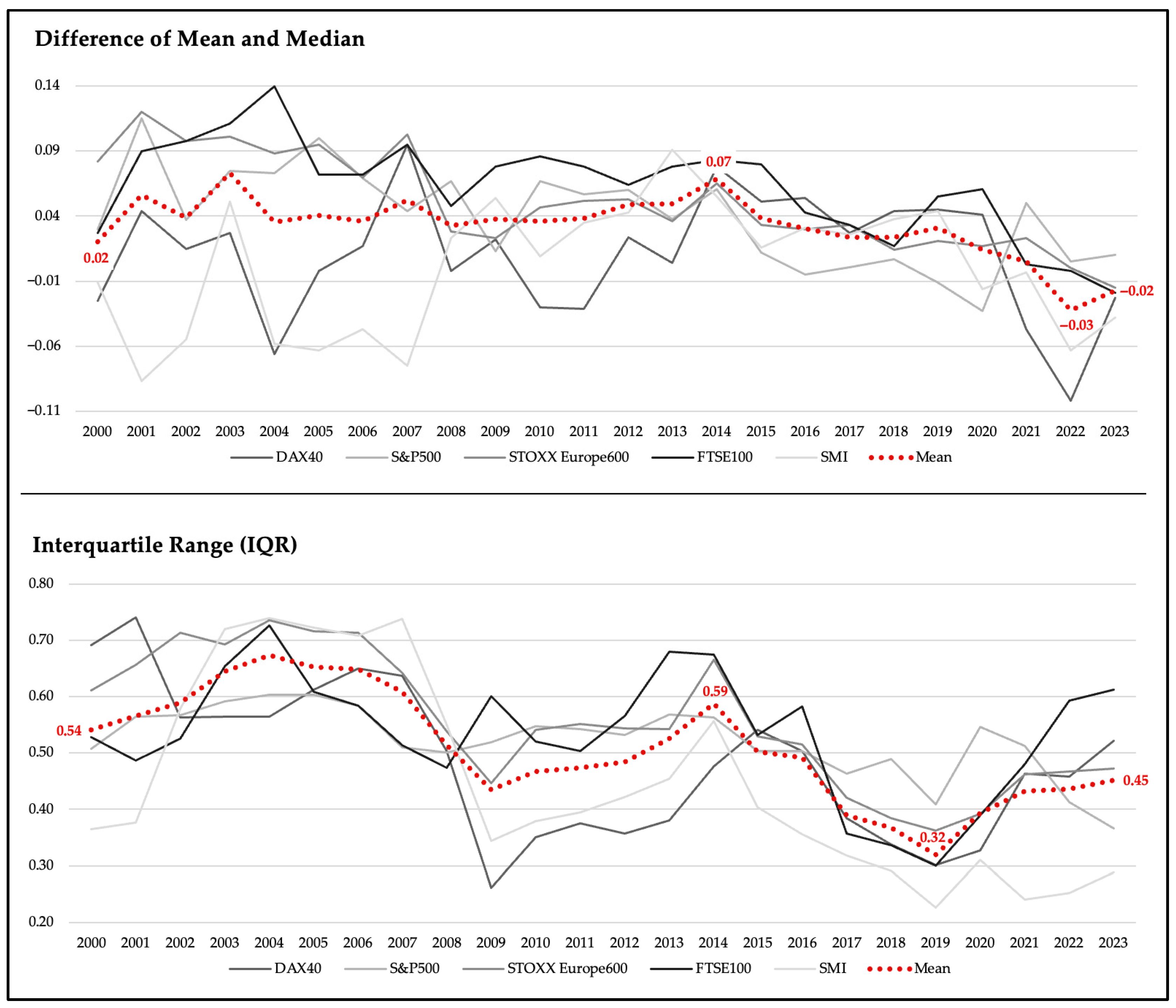
Figure 5 presents the empirical evidence depicted through the mean-median difference, which measures skewness of beta distributions, and the IQR, which measures dispersion. From an investor’s perspective, increases in both parameters would indicate higher systematic risk, while decreases would indicate reduced risk exposure. A positive mean-median difference (mean
median) indicates right-skewed distributions, reflecting a subset of high-beta firms with above-average market sensitivity that increases the distribution mean. Conversely, a negative difference (mean
median) indicates left-skewed distributions, reflecting a preponderance of low-beta firms with below-average market sensitivity.
Linear regression analysis of these distributional indicators across the 2000 to 2023 period reveals regression slopes of −0.0021 and −0.0105, providing quantitative evidence that systematic risk exposure did not increase over the study period. Instead, the results indicate declining volatility of company share prices relative to index level movements, suggesting reduced systematic risk exposure for investors.
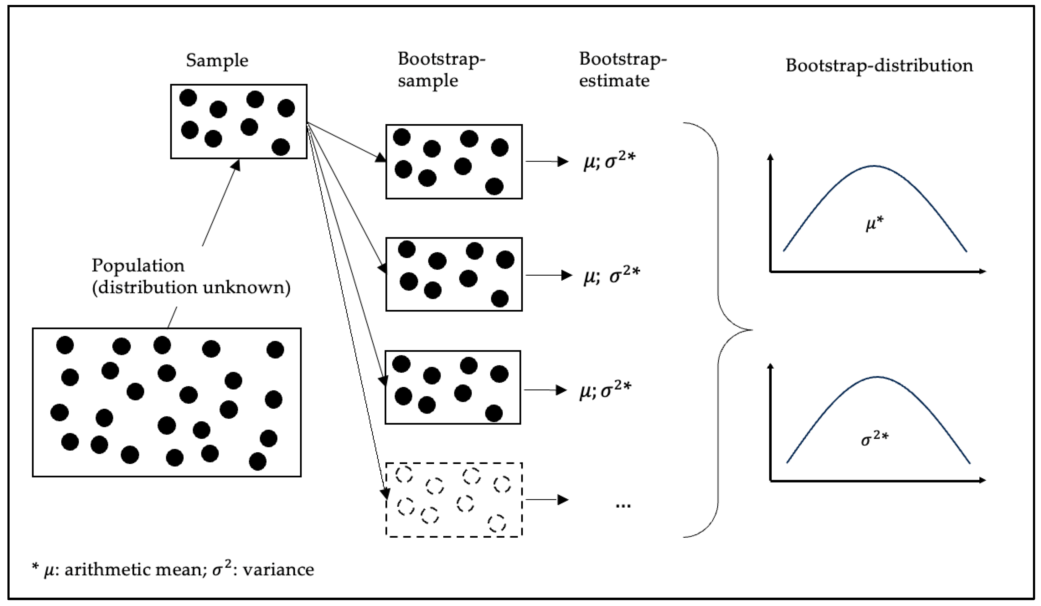
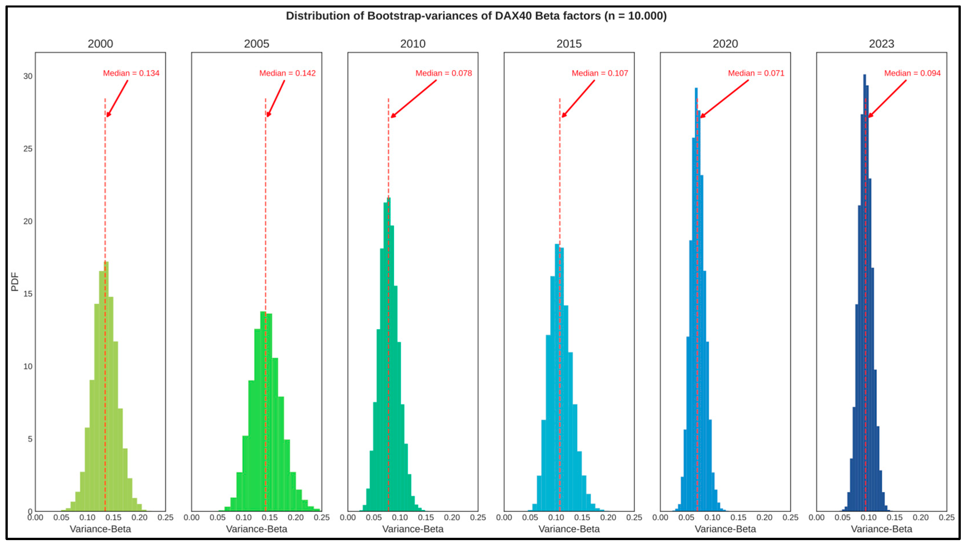
With bootstrap analysis, 10.000 variance beta estimates are generated through random sampling with replacement for each year’s cross-sectional beta distribution. The median of bootstrap variances provides a robust, non-parametric estimate of the central tendency of year-specific beta factor variance. Across the period of 2000 to 2023, 24 bootstrap estimates are generated to produce a time series of median bootstrap variances.
Figure 6 presents the results for DAX40 companies as an illustrative example.
The empirical evidence reveals two critical findings: (1) the median bootstrap variance of DAX40 beta factors decreased substantially from 0.134 in 2000 to 0.094 in 2023, representing a 29.9% reduction in systematic risk dispersion over the 23-year period. (2) The progressive decline in median bootstrap variance indicates that the cross-sectional spread of systematic risk exposures among firms has narrowed, suggesting more homogeneous market risk profiles and reduced environmental shocks affecting individual firms.
Figure 7 shows the development of the medians of the beta variances of all indices over time and provides evidence for decreased beta factor variances across all indices. On average, from 0.176 (in 2000) to 0.103 (in 2023)—this corresponds to a reduction of 41.5%. From an investor’s perspective, this convergence in systematic risk exposures indicates a more stable or less turbulent equity market environment during the investigation period.
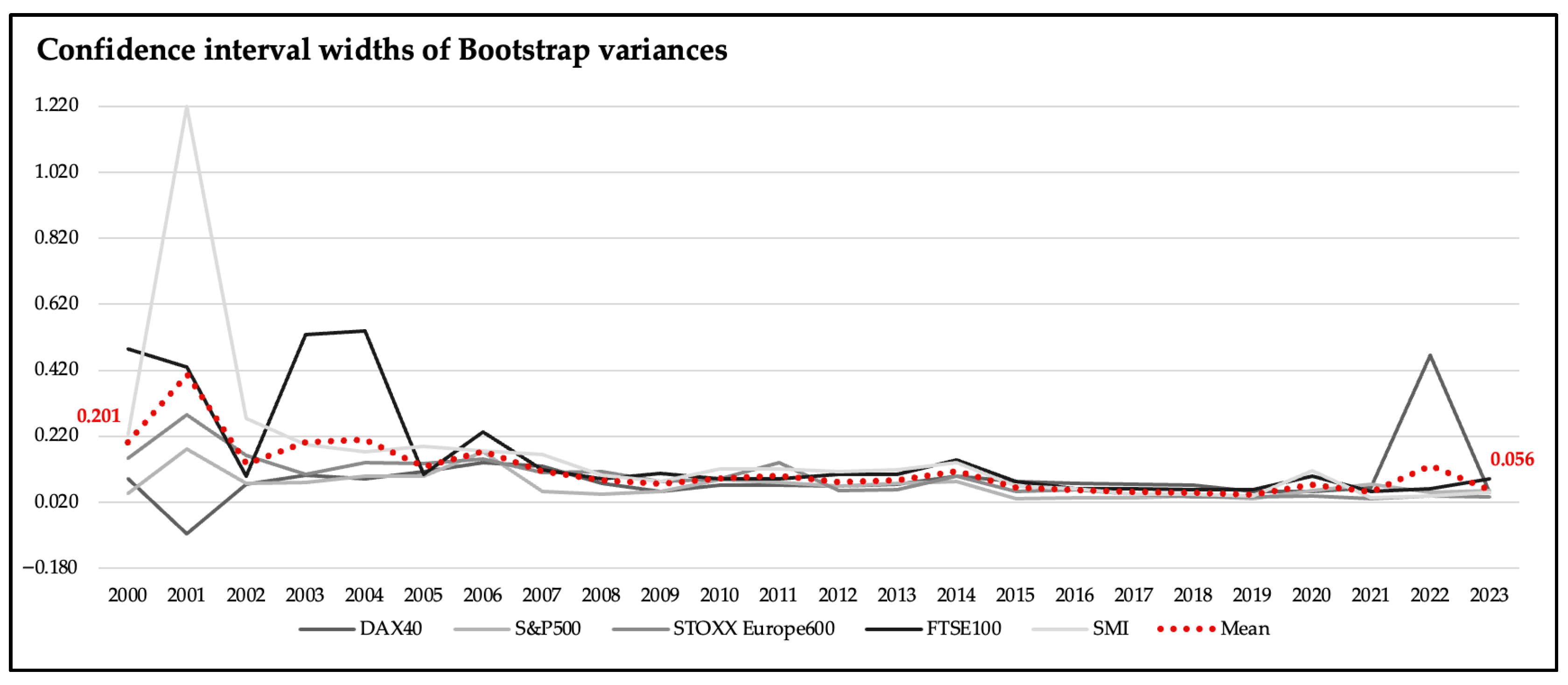
To assess the precision and variability of beta factor variance estimates, 95%-bootstrap confidence intervals are constructed for each year’s beta factor distribution. The confidence interval width provides a quantitative measure of the dispersion of bootstrap variance estimates. Consistent with the median-variance findings, the confidence interval widths demonstrate a significant decline (see
Figure 8; see
Table 4). This convergence of confidence interval widths indicates reduced variance in systematic risk exposure and provides additional statistical support for the conclusion that cross-sectional beta factor variability has declined over time.
The bootstrap hypothesis testing compares the 2023 beta distribution against each prior year (2000 to 2022). Empirical p-values derived from 10.000 bootstrap samples range from 0.45 to 0.60 across all indices. These p-values significantly exceed the conventional significance threshold , providing strong statistical evidence that the null hypothesis cannot be rejected. This result indicates no statistically significant increase in 2023 beta factor variances relative to prior years, thereby supporting the conclusion that systematic risk exposure has not increased over time.
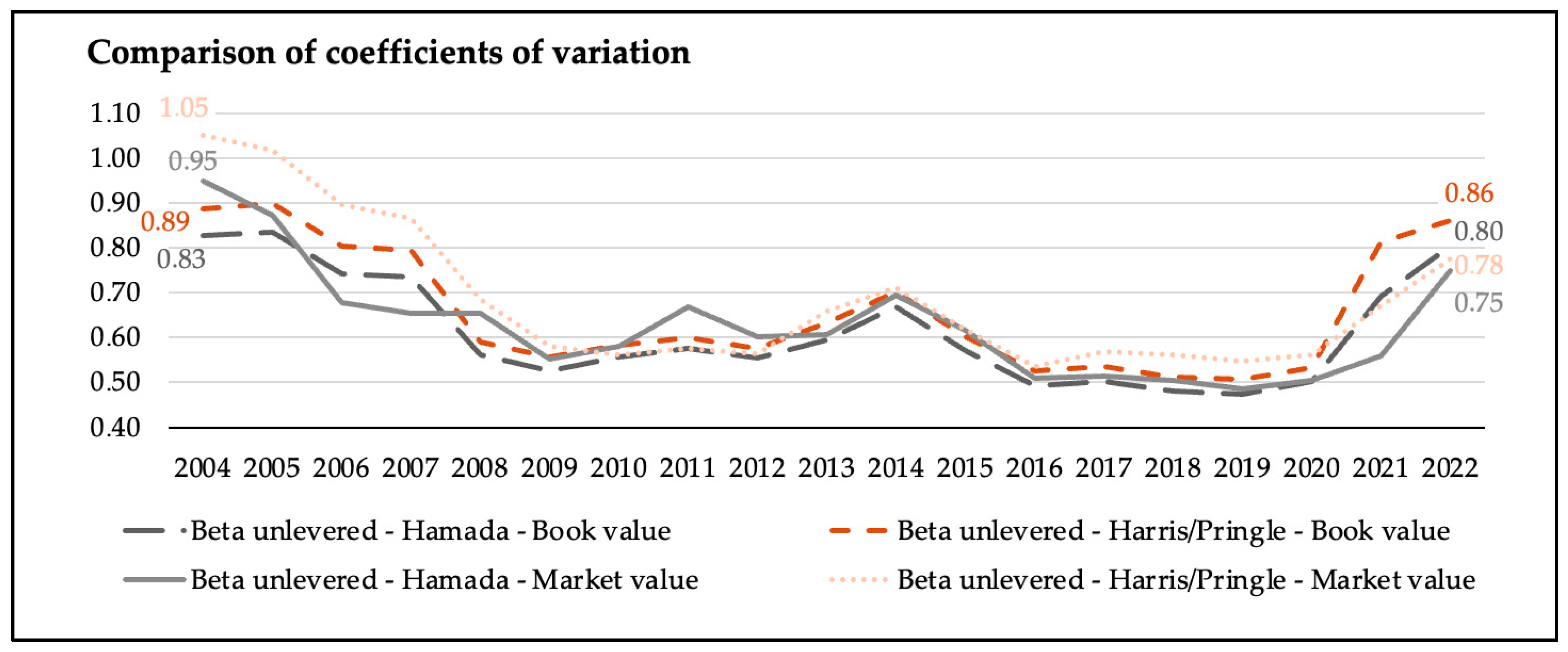
The unlevering procedures according to Hamada and Harris/Pringle are applied to isolate systematic business risk from financial leverage effects.
Figure 9 presents the temporal development of unlevered beta coefficients of variation (CV) and variance measures. The results reveal contrasting patterns across the study period: from 2000 to 2020, both CV and variance measures demonstrate declining trends, indicating reduced variability in unlevered systematic risk exposure. However, from 2020 to 2022, both metrics increased sharply, which may be attributable to the greater uncertainty associated with the COVID-19 pandemic. Therefore, unlevered beta factors exhibit no systematic increase that could explain persistent WACC levels. An adjustment for financial leverage through unlevering procedures does not alter the conclusion derived from levered beta analyses.
Discussion in the context of the research question. Observable systematic risk cannot explain WACC persistence. Distributional and bootstrap analyses reveal declining skewness, compressed IQR, and 41.5% variance reduction—indicating reduced, not increased, risk. Unlevered beta analyses corroborate these findings. Consequently, hypothesis H1 is falsified.
4.2. H2: Overall Market Risk Exposure: Volatility Analyses
Market volatility is examined using distributional analysis, regression analysis of dispersion statistics, and retrospective evaluation of historical volatility as a predictor of investor risk expectations.
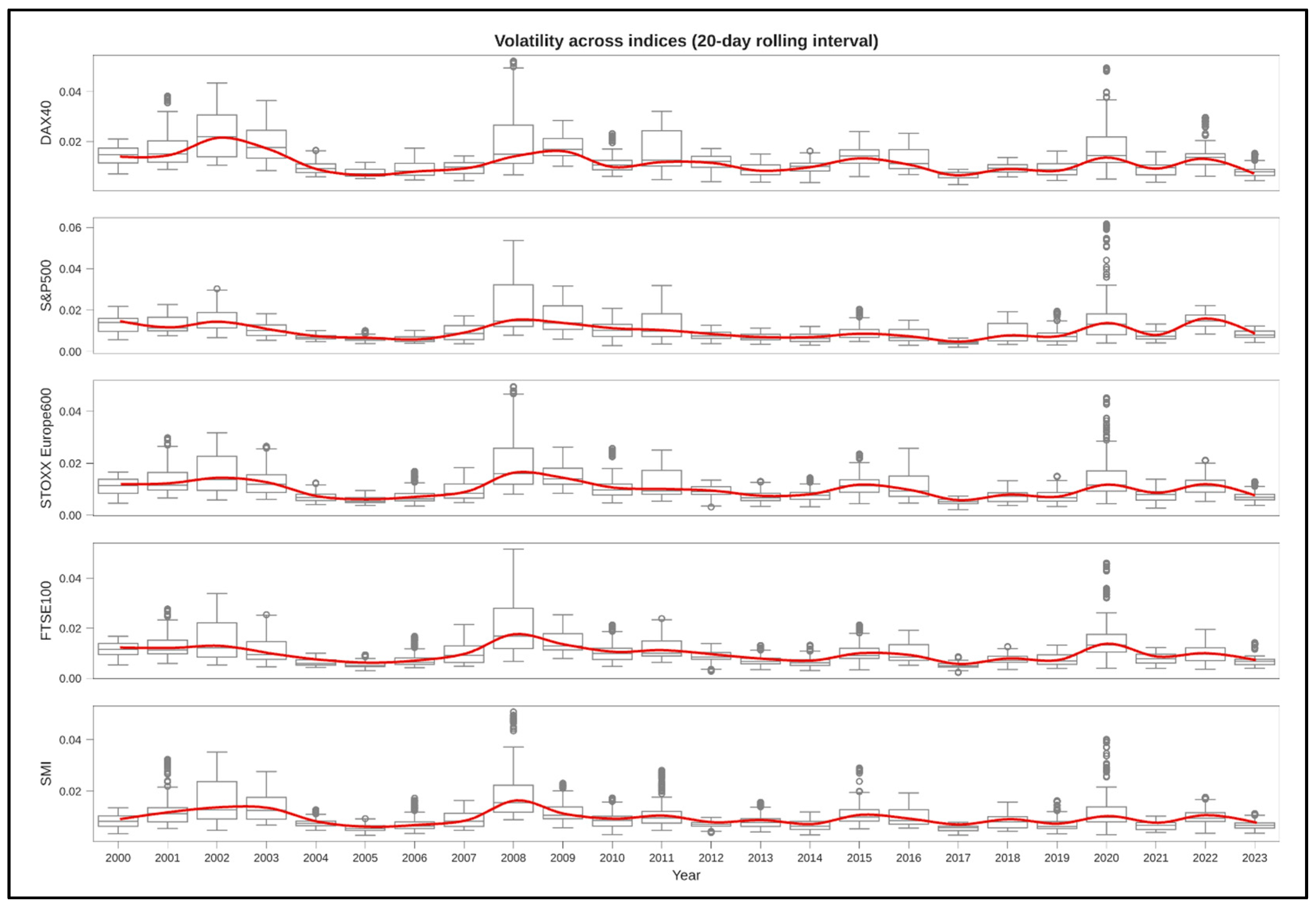
Figure 10 presents box plots illustrating volatility distributions across indices. The figure reveals positive outliers concentrated in three distinct periods: the 2008 global financial crisis, the 2020 COVID-19 pandemic, and the 2022 geopolitical tensions surrounding the Russia-Ukraine conflict. Abstracting from these exogenous shocks, volatility data demonstrate a consistent decline since 2008.
Linear regression of distributional statistics provides quantitative support for declining market risk exposure (
Table 5). The median and IQR both exhibit negative regression slopes across the 2000–2023 period, indicating a continuous decline in the central tendency and spread of volatility. The coefficient of determination R
2 ranges from 0.063 to 0.166 for median and IQR measures, reflecting a moderate linear fit. In contrast, the number of outliers exhibits a positive regression slope, primarily driven by the pronounced volatility events of 2008–2011 and 2020–2022. However, the R
2 for outlier frequency is substantially lower (R
2 < 0.10 across indices), indicating that outlier frequency explains less than 10% of temporal variation. This asymmetry suggests that while extraordinary market events have created isolated peaks in outlier occurrence, the secular trend in market volatility remains decidedly downward. Thus, overall market risk exposure, as measured through volatility, fails to explain persistent WACC levels in the 2004–2021 period.
Retrospective analysis and volatility buffer construction. Retrospective volatility analysis compares historical volatility forecasts (5–10 year averages) to realized volatility. Positive volatility buffers (historical > realized) indicate conservative estimation.
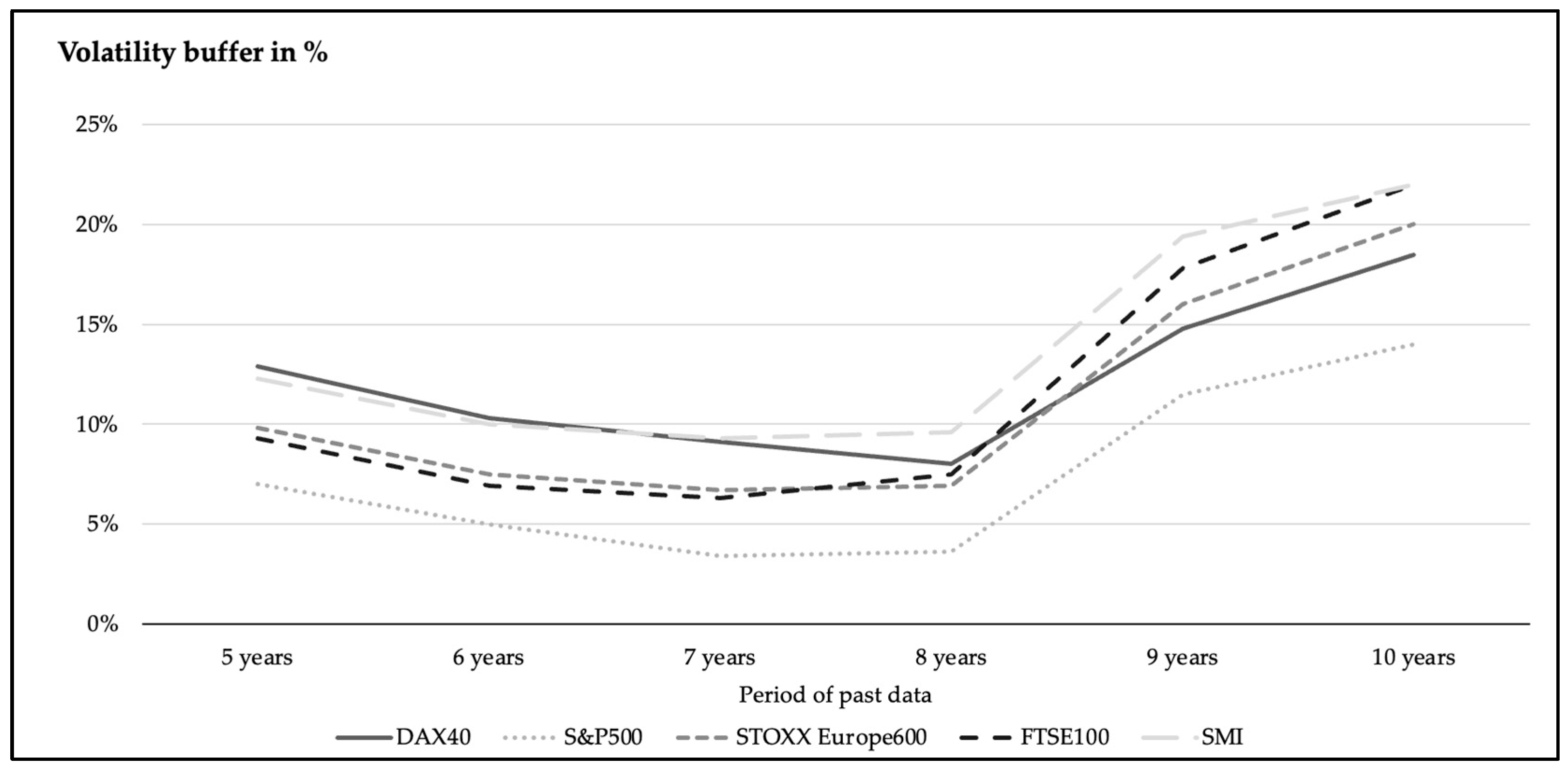
Figure 11 depicts average volatility buffers as functions of the historical observation period. It shows that longer historical windows tend to yield higher expected volatility estimates relative to realized outcomes. Intuitively, investors utilizing longer historical periods incorporate greater safety margins, ensuring to be on the ‘safe side’, as the expected volatility exceeds actual volatility to protect against adverse surprises. The decline of volatility buffers from five to eight years of return length is attributed to increased volatility due to the COVID-19 crisis. The theoretical implications are worth stating explicitly: If historical volatility is an adequate substitute for expected volatility, no additional risk premium adjustments would be economically rational. In addition, a constant or increasing volatility buffer may indicate a reduction in the overall market risk exposure.
An example of buffer values illustrates the practical implications. A practitioner who estimates the expected volatility of the DAX40 based on a five-year historical interval would specify volatility expectations that are, on average, 12.9% higher than the volatility subsequently realized. Using a ten-year historical period increases this conservative bias to 18.5%, showing that longer observation periods tend to lead to higher volatility buffer ratios.
Table 6 provides cross-sectional evidence regarding positive buffer frequency across indices and observation intervals. Data reveals that positive volatility buffers occur in an average of 69.7% of cases, whereas negative buffers occur in 30.3% of cases.
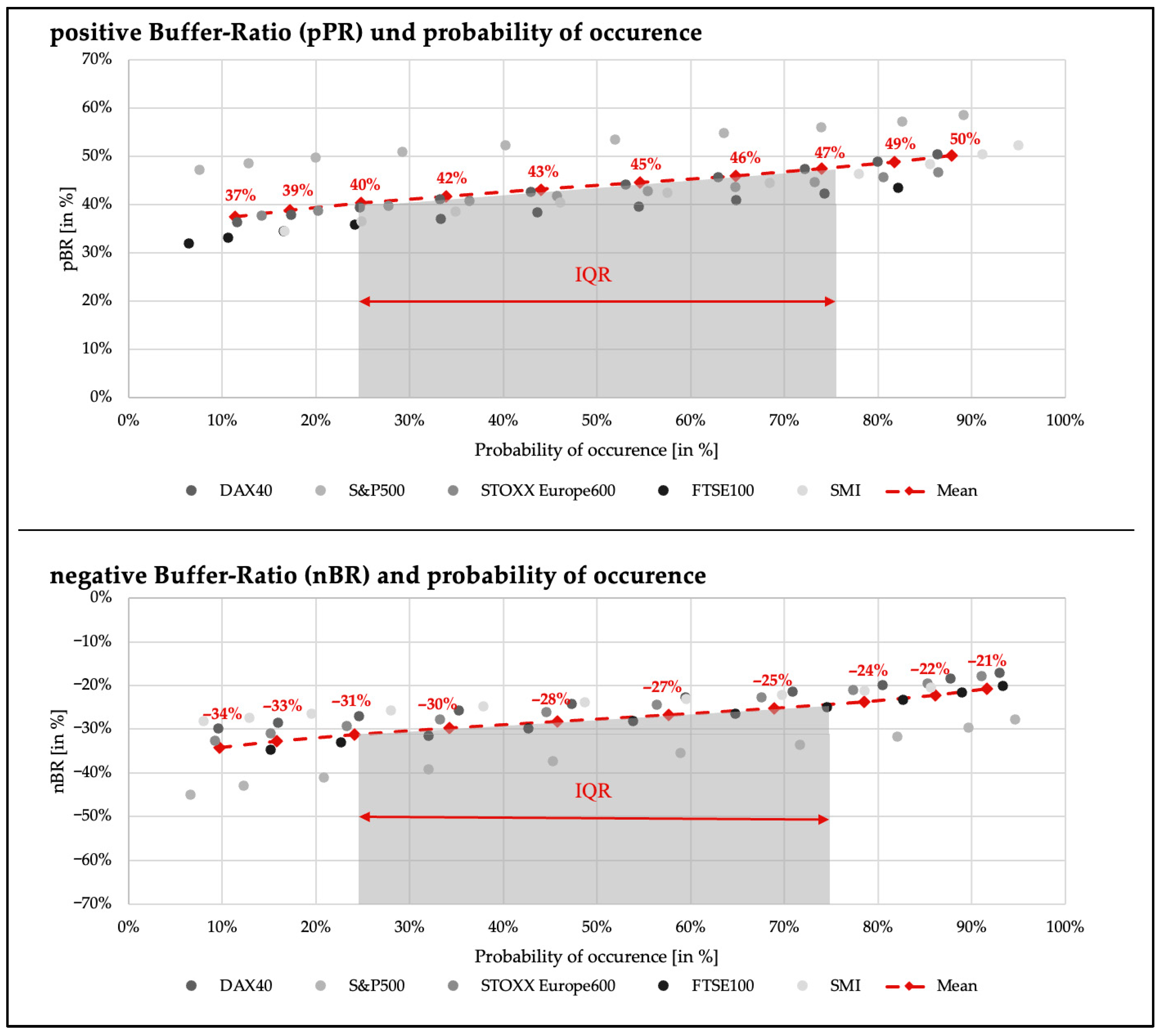
Shortfall risk is relevant for investors and practitioners. Although average volatility buffers are positive, the distribution of these buffers exhibits asymmetry. To quantitatively investigate this observation, a comparison is made between relative negative (nBR) and relative positive (pBR) volatility buffer ratios. Kernel density estimations (KDE) show that positive buffer ratios (pBR) exhibit a concentrated distribution with maximum density at 58% and a modal value near 45%, indicating that in typical years, forward forecasts exceed realized volatility by this magnitude. In contrast, negative buffer ratio distributions (nBR) are more dispersed and attenuated, averaging between −34% and −21%.
This asymmetry indicates that downside shortfall risk—situations where forecasts underestimate realized volatility—occurs less frequently and with smaller magnitude than upside buffer opportunity. IQR quantifies this asymmetry. For pBR, the central 50% of observations fall between 40% and 47%, indicating conservative bias in forecasting. For nBR, the IQR spans −31% to −25%, demonstrating a narrower range of downside deviations. This observation confirms that the shortfall risk is lower than the upside opportunity (see
Figure 12).
Discussion in the context of the research question. Distributional analysis reveals a monotonic decline in market risk exposure, falsifying claims that rising volatility compensates for lower rates. Historical volatility forecasts exceed realized values in 69.7% of cases with no temporal increase in buffer magnitude. Upside opportunity (+44%) exceeds shortfall risk (−27.5%) by 16.5% at 50% probability. Consequently, hypothesis H2 is falsified: observable volatility metrics provide no explanation for WACC persistence.
4.3. H3: Market Price of Risk: Lambda Factor Analyses
Because lambda is only one among several possible proxies for time-varying equity risk premia and is known to be sensitive to return horizon and measurement choices, the following analysis should be viewed as exploratory rather than as a central test of practitioner risk-aversion dynamics. This subsection assesses temporal trends in lambda factors to evaluate whether increasing investor risk aversion constitutes a plausible explanation for persistent WACC levels. The market price of risk (lambda factor) quantifies investor risk aversion, representing the additional return required per unit of risk exposure.
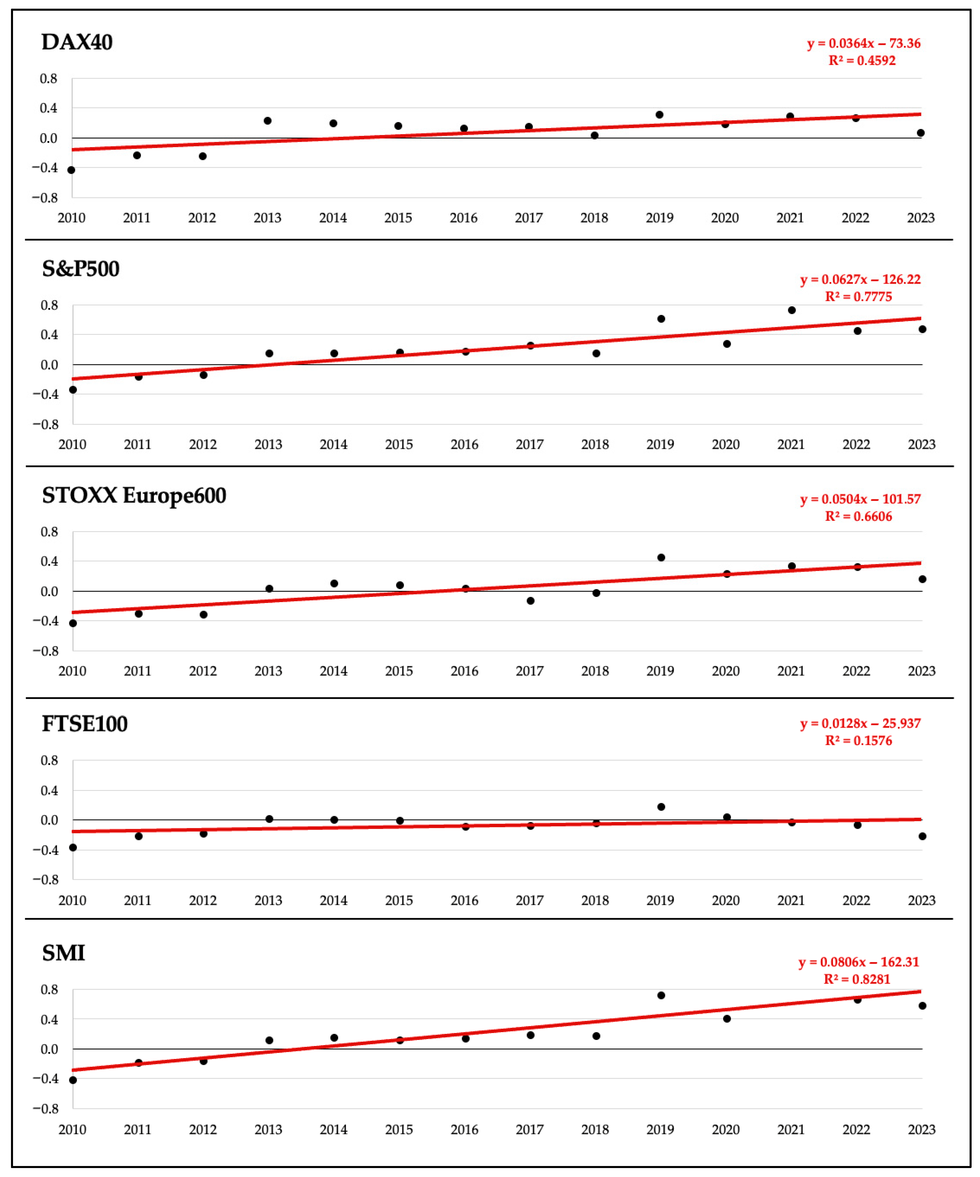
Linear regression analysis reveals positive growth in lambda factors across all indices between 2010 and 2023, with annualized increases ranging from 1.28% (for FTSE100) to 8.06% (for SMI). However, two methodological limitations warrant attention. First, negative lambda values emerge for all indices during 2010–2012, presenting an interpretive challenge. Since lambda is defined as the ratio of market risk premium to volatility, negative lambda values arise when the numerator is negative—that is, when the ten-year geometric mean market return is negative despite positive risk-free interest rates. Under the risk-return theory, negative market risk premiums are economically implausible. For example, the DAX40 in 2010 exhibited a ten-year geometric mean return of −4.75%, with a contemporaneous ten-year German government bond yield of 2.78%, yielding an implied market risk premium of −7.53%. With an annualized volatility of 17.58, this produces a negative lambda factor, which contradicts fundamental financial theory stipulating positive risk compensation. Accordingly, removing observations with negative lambda factors due to their lack of being theoretically plausible, the following adjustment lines result (see
Figure 13).
Excluding negative lambda values yields significantly weaker upward trends in lambda factors. Given lambda’s sensitivity to the market return interval specification, a formal sensitivity analysis is necessary to establish the robustness of trend conclusions (see
Table 7).
The sensitivity analysis systematically varies the market return interval from ten to 15 years, evaluating the lambda factor sensitivity to this methodological choice.
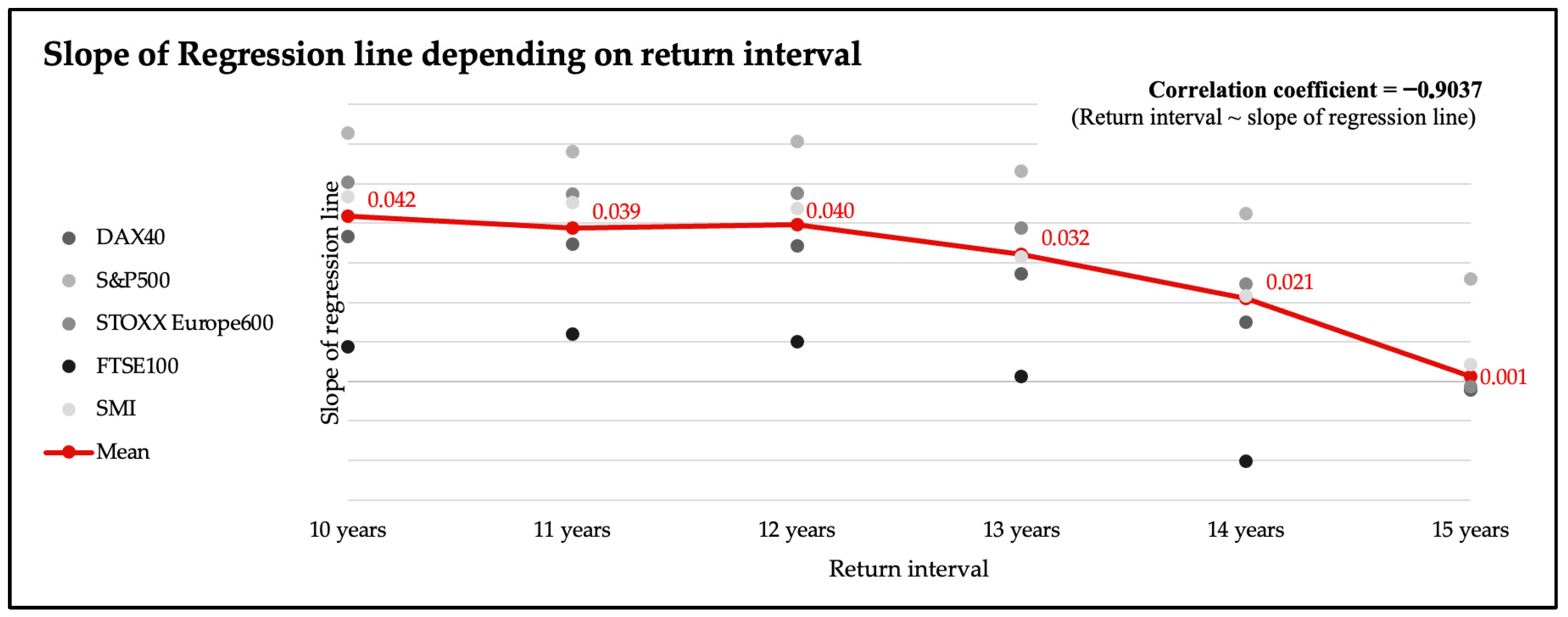
Figure 14 plots regression slope coefficients as functions of interval length. Across all indices, a strong negative relationship exists: Lambda factors average 0.042 for ten-year intervals, decline to approximately 0.021 for 14-year intervals, and approach 0.001 for fifteen-year intervals (Pearson correlation = −0.9037, indicating strong negative dependency). Thus, the sensitivity analysis reveals that empirical conclusions regarding lambda factor trends depend critically on the length of the return interval.
Discussion in the context of the research question. Given the pronounced methodological sensitivity of estimated lambda factor trends to the specified return interval, the lambda analysis indicates that in some specifications the market price of risk appears to increase over time, but this conclusion is not robust to reasonable variations in the return interval and the treatment of periods with negative market risk premia. Given this methodological fragility, H3 cannot be decisively accepted or rejected, and the lambda results are interpreted only as suggestive diagnostics that motivate further research on equity risk-premium dynamics.
4.4. H4: Earnings Risk: EBIT Volatility
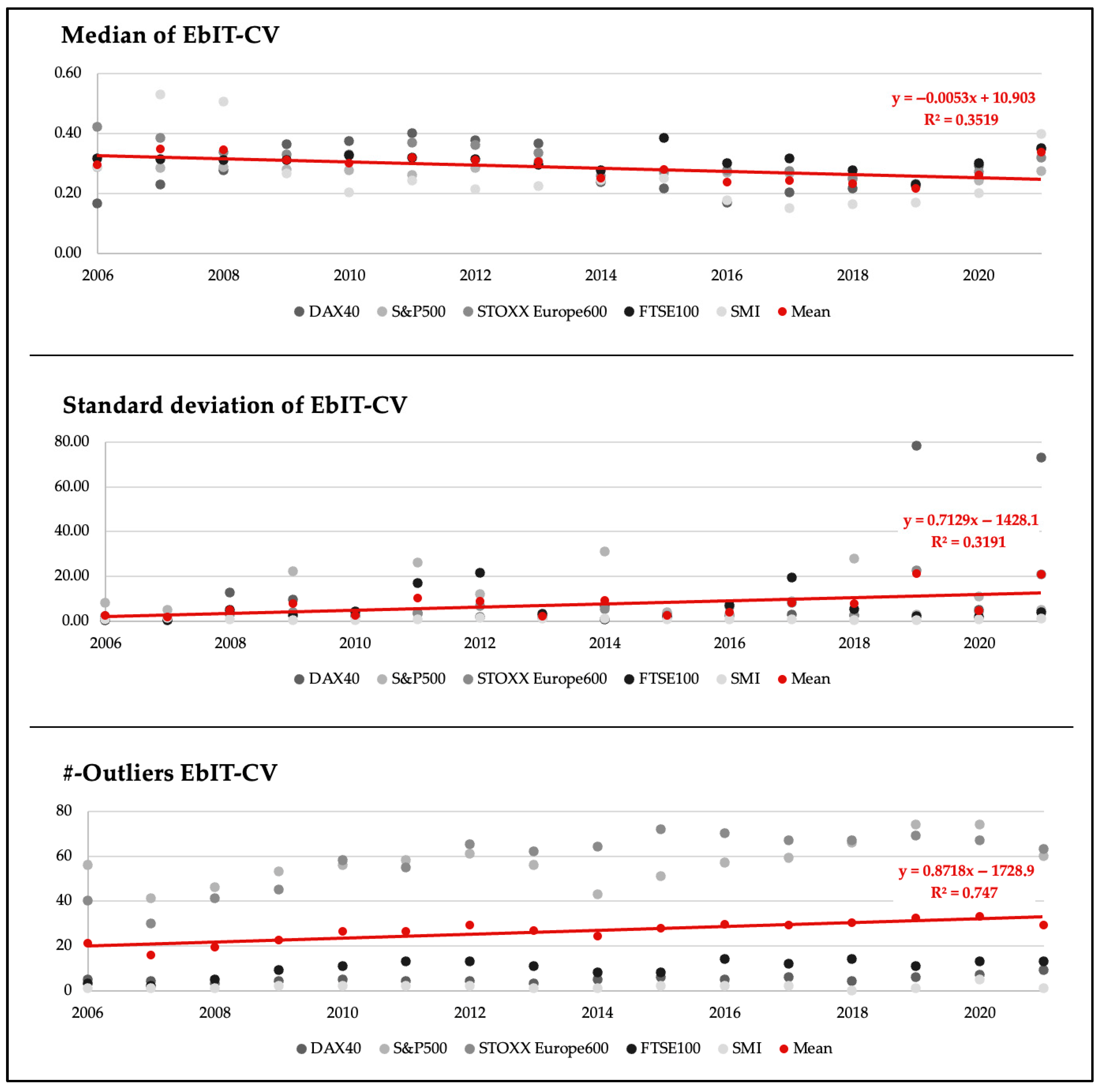
In line with the previous analyses, linear regression of distributional statistics investigates median, standard deviation, and number of outliers. The analysis spans from 2006 to 2021 due to data availability constraints for DAX40 companies prior to 2006. The median CV exhibits a negative trend of −0.0053, indicating a declining central tendency of earnings volatility over 15 years. This negative slope is driven predominantly by the 2011–2019 period. However, median CV values increased during 2020–2021, reaching levels observed during the 2008–2010 financial crisis, suggesting cyclical earnings volatility patterns (see
Figure 15).
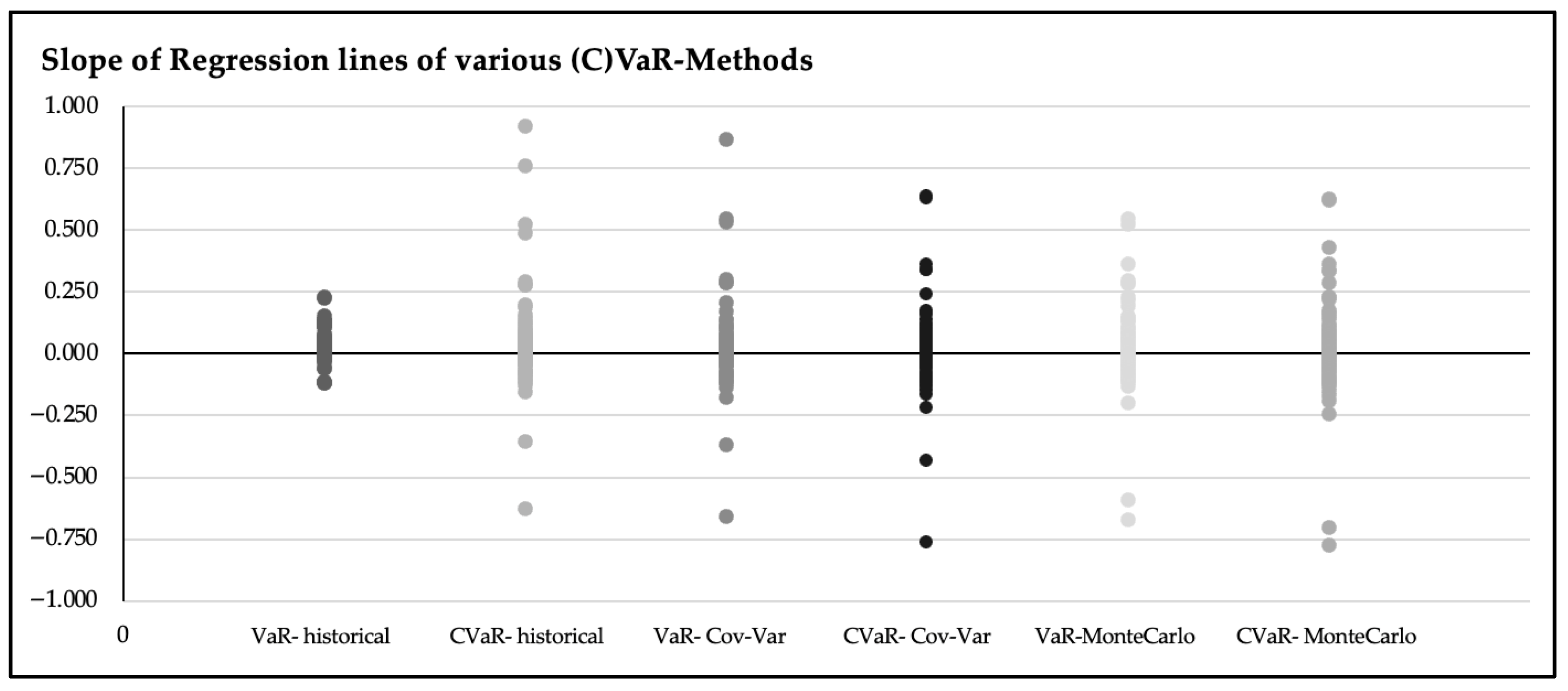
Standard deviation of CV (slope = 0.719) and outlier frequency (slope = 0.8718) are driven by two extreme values (78.33 in 2019, 72.76 in 2021). Excluding these reduces the standard deviation slope to 0.194, confirming median CV as the robust measure. This supports declining earnings volatility trends. Return-VaR and -CVaR are estimated across three methodological approaches: historical simulation, variance-covariance, and Monte Carlo methods. The analyses result in 6588 slopes for the shortfall measures’ regression lines capturing the temporal trend in return-(C)VaR (see
Figure 16).
Positive regression slopes indicate increasing return-(C)VaR, implying that companies have risen EBIT margins in downside scenarios (worst 5% of cases) over time and consequently improved financial performance, even under adverse conditions.
In total, 68.6% of regression slopes are positive, suggesting that in the majority of cases, return-(C)VaR measures demonstrate upward trends. This pattern corroborates the median CV finding, namely that earnings volatility has generally declined, contradicting any claim of increased earnings risk.
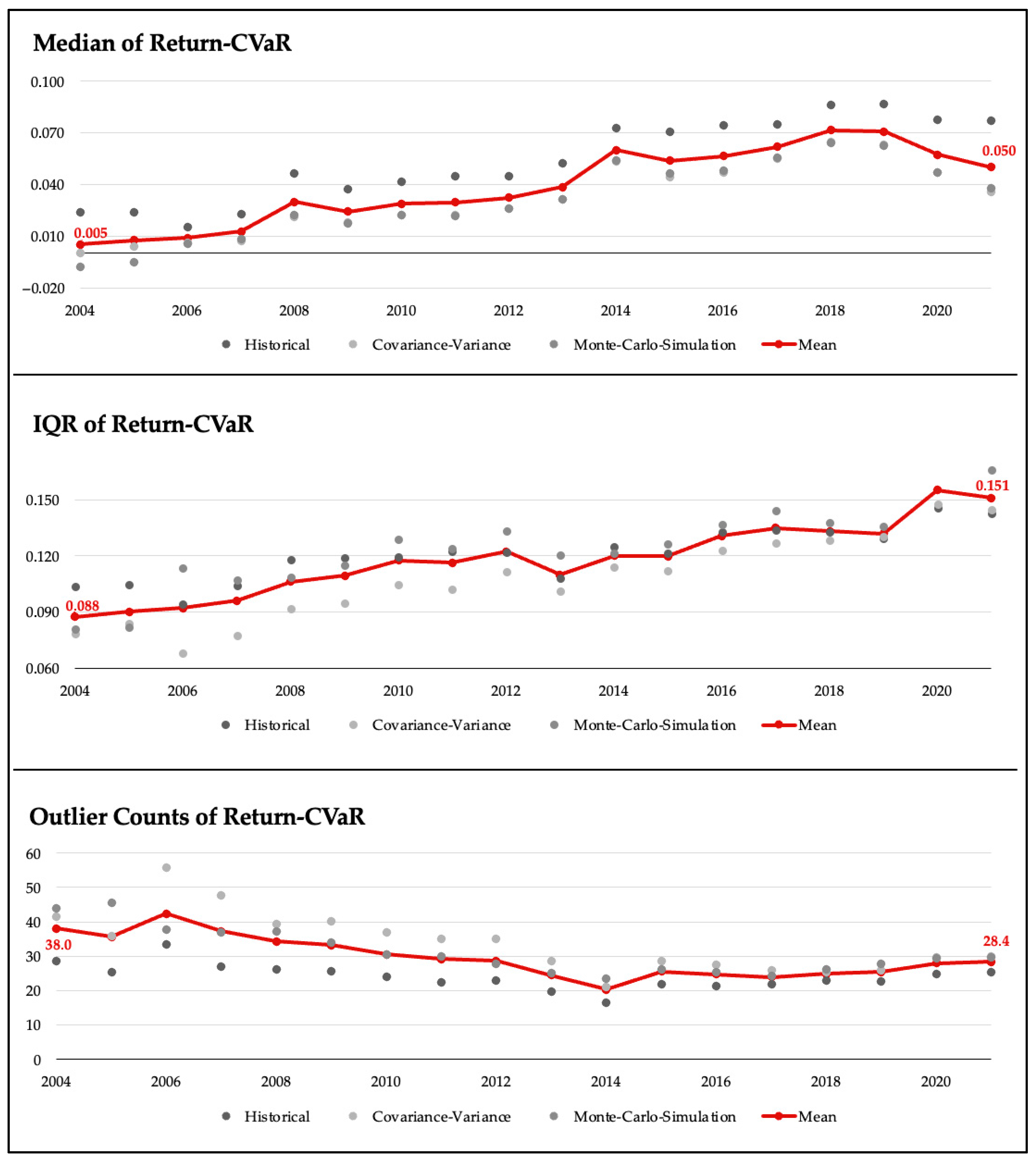
Figure 17 presents return-CVaR statistics across all five indices over the 2004–2021 period. The median return-CVaR increased significantly, rising from 0.5% in 2004 to 5.0% in 2021—a tenfold increase reflecting improved downside earnings performance. Since higher return-CVaR thresholds indicate that worst-case EBIT scenarios have improved, this pattern signals reduced earnings risks. However, the IQR expanded 71.6% over the same period. This noticeable contradiction resolves upon examination: the IQR expansion reflects rightward distribution shift rather than tail-risk deterioration. Specifically, the 75th percentile return-CVaR quantile increased due to higher average return-CVaR values across firms, not due to the emergence of negative outliers or distribution deterioration.
Discussion in the context of the research question. Multiple analytical approaches confirm no systematic increase in earnings risk. Median CV declined, negative EBIT frequencies diminished, and 68.6% of return-(C)VaR regression slopes were positive, indicating improved downside performance across all methods. Thus, hypothesis H4 is falsified: observable earnings risk metrics provide no explanation for the WACC phenomenon.