Revisiting a Post Keynesian Explanation of US Inflation

Abstract

This paper presents an econometric analysis of inflation from a Post Keynesian perspective using quarterly data from 2002 to 2024 for the United States, including the most recent period of inflation after the onset of the COVID-19 pandemic. I evaluate the continued relevance of the comprehensive Post Keynesian model of inflation using a reduced form equation that incorporates both the aggregate demand–augmented wage-cost markup equation and the wage growth equation which is robust in explaining inflation. The robustness of the model is tested by incorporating different measures of labor market slack, wages, and inflation. The paper finds that the comprehensive model is not robust for the period 2002 to 2024 even when alternative measures for wages, unemployment, and inflation are utilized. This discrepancy arises because the negative relationship between unit labor costs and inflation, observed in the updated model, proved non-robust upon the inclusion of control variables for energy costs and imports. After employing the Prais–Winsten estimation to account for persistent serial correlation, the revised model aligned with the sign conventions of the original Atesoglu wage-cost markup equation. Specifically, while the coefficient for unit labor costs turned positive, it failed to reach statistical significance. Finally, I discuss potential factors for the decrease in the magnitude and significance of the coefficients in the aggregate demand–augmented wage–cost markup model for the period 2002 to 2024 as well as the pass through of wage growth to broader inflation measures.

1. Introduction

In recent decades, there has been an intense debate about the causes of inflation. The debate has gained steam in recent years due to the acceleration of prices following the COVID-19 pandemic and subsequent research on “greedflation” (Weber & Wasner, 2023).

The importance of this debate cannot be understated, since inflation, if it is not matched by proportional changes in nominal wages, erodes the purchasing power of consumers. A broader concern is that inflation triggers a response by the central bank in terms of contractionary monetary policy due to its price stability mandate.

The actions of the central bank have implications for the labor market in the form of a higher unemployment rate and slower wage growth. Therefore, a complete understanding of the cause of inflation is paramount to maintaining the health of the labor market and the overall economy.

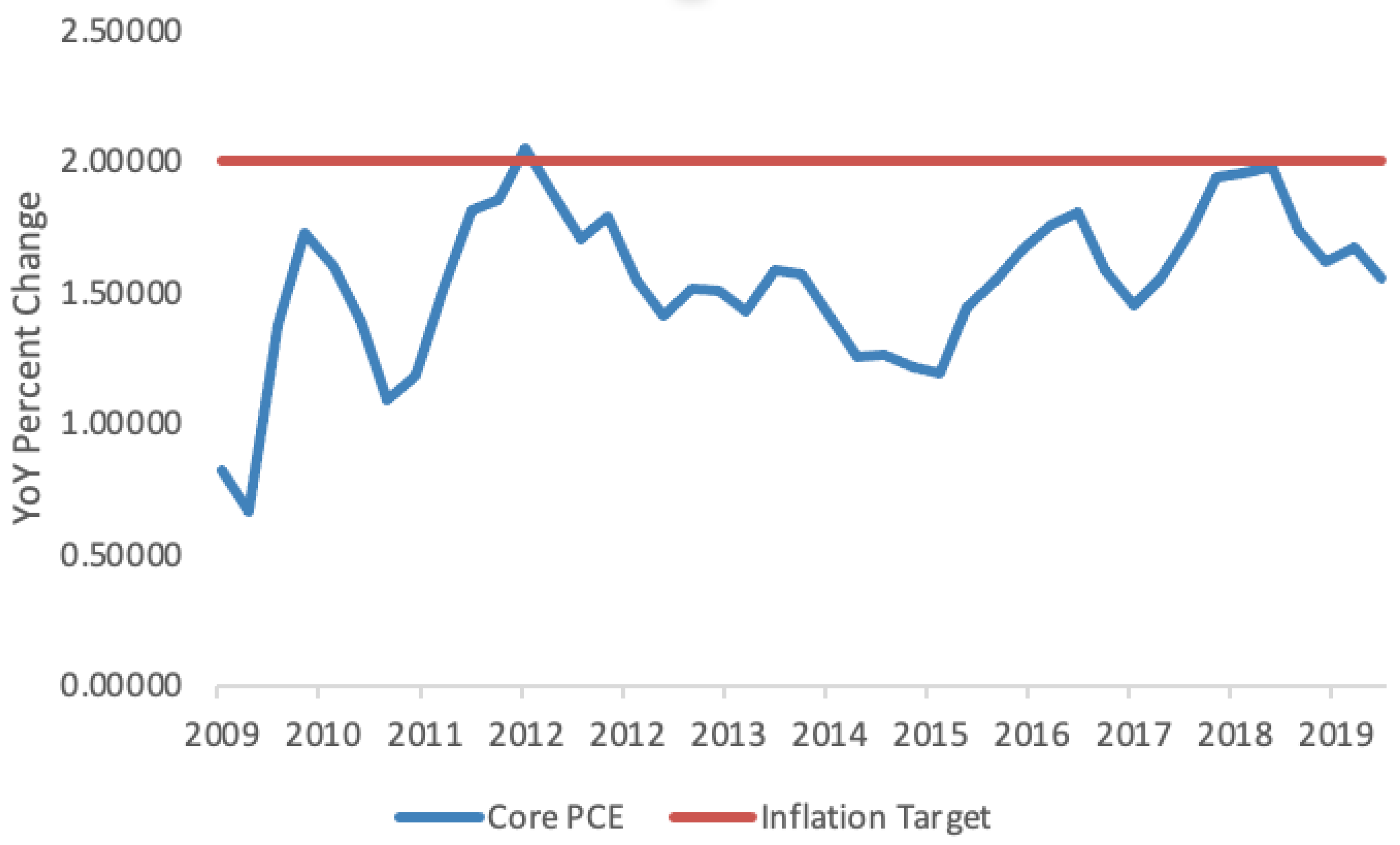
The US economy has changed dramatically since Atesoglu first raised the issue of the causes of inflation. The IT revolution that ushered in the productivity boom of the 1990s and the accelerated economic growth that accompanied it faded by the end of 2007 in the wake of the housing crash and the ensuing financial crisis. GDP growth slowed considerably from its pre-recession trend during the initial phase of the recovery in June 2009. However, the United States experienced incredibly low unemployment, but this did nothing to boost inflation, which hovered at or below two percent for much of the recovery from the financial crisis up to the point of the recession caused by COVID-19 as seen in Figure 1.

The combination of low unemployment and low inflation in the US has led many economists to declare that the Phillips curve is dead. Borio and Gambacorta (2017) proclaimed that “the response of inflation to a measure of labour market slack has tended to decline and become statistically indistinguishable from zero” (Borio & Gambacorta, 2017). This is an important conclusion, because Atesoglu (1997) incorporates an equation in which wages are a function of unemployment and inflation. This is very similar to the original Phillips curve, which regressed the rate of change of money wages on the unemployment rate in the UK for the period 1960 to 1969.

Atesoglu (1997) found that a wage-cost markup model1 as referenced in Downward (1994) combined with a Phillips curve-inspired wage growth equation forms a comprehensive model that is robust in explaining inflation from a Post Keynesian perspective. This seems to be in stark contrast to conventional wisdom regarding the current state of the Phillips curve relationship.

A key question to ask is “why has the slope of the Phillips curve flattened? This question is extremely important to answer for many Post Keynesians because inflation is assumed to be a conflict problem between workers and firms rather than a monetary phenomenon, as described by Milton Friedman invoking Irving Fisher’s quantity theory of money.

The core idea behind a conflicting claims approach to inflation is that both “workers and firms care about achieving “fair” shares of total income and will strive to inflate nominal wages and prices, respectively, in accordance with the disparity between these fair shares and the actual wage share” (Setterfield, 2006). A key point regarding nominal wage growth that is often overlooked is that it should exceed the inflation rate by the rate of growth of labor productivity (assuming that the latter is greater than zero). This is an important point because wages can rise faster than prices without the former becoming inflationary or igniting a wage–price spiral.

Setterfield (2006) provides a compelling explanation for the flat Phillips curve. Using a Conflicting Claims Model (Rowthorn, 1977; Lavoie, 1992), he describes a situation where bargaining power (which is a function of both unemployment and labor market institutions that impact worker income insecurity) increases as a result of a decrease in the unemployment rate. At the same time, there could be a decrease in union density, which would decrease bargaining power. The magnitude of each of these impacts must be the same in order to offset each other and generate a flat Phillips curve (Setterfield, 2006).

Herdelin (2025) draws a similar conclusion to Setterfield (2006) by analyzing periods of negative unemployment rate gaps, which are described as periods when the unemployment is below the non-accelerating inflation rate of unemployment or NAIRU.2 Negative unemployment rate gaps3 result in increased bargaining power for workers, as firms offer higher wages to poach workers from other firms as labor becomes more scarce (Herdelin, 2025).

A major problem that has emerged since Atesoglu (1997) is that the headline unemployment rate has diminished as a measure of slack in the labor market. As more and more people give up looking for work and exit the labor force, the headline unemployment rate loses explanatory power. Alternative measures of slack in the labor market could better inform policymakers about the overall health of the labor market.

This paper begins with an investigation of the robustness of the results found in Atesoglu (1997). Specifically, it investigates whether the headline unemployment rate adequately measures the amount of slack in the economy, whether there are more comprehensive measures of wage growth, and whether the correct measure of inflation is being used if we are to estimate a Phillips curve-inspired wage growth equation as referenced in Atesoglu (1997).

These challenges were highlighted in Cornwall and Cornwall (2001) and again in Setterfield (2006), “Some authors argue that measurement problems have resulted in US unemployment rates being understated over the past fifteen years” (Cornwall & Cornwall, 2001) as cited in (Setterfield, 2006).

The subsequent work in this paper will be to update the existing model to estimate a new wage growth equation using alternative measures of compensation, the unemployment rate, and inflation in an effort to correct inherent measurement problems and assess whether the original Atesoglu (1997) comprehensive model is robust for the period 2002 to 2024.

The remainder of the paper is organized as follows. Section 2 begins with comments on the longer-term context in which the study is conducted. In Section 3, the original Atesoglu model is presented and key departures from the model are explained. Section 4 discusses the econometric results for each of the models discussed in the paper. Section 5 summarizes the findings of the paper and how they relate to the ongoing debate surrounding the flattening of the Phillips curve in the US. Section 6 provides concluding remarks.

2. Background

As compared to the inflation-ridden 1970s and 1980s, inflation from 1990 onward in the US has fallen to low levels not seen since the end of the post-war (1950s/60s) Golden Age. The inflation rate (as measured by the PCE) peaked in 1980 at 11.6 percent, but by 1990 had declined to 5.1 percent. The inflation rate continued to decline throughout much of the 1990s, hitting a trough of 0.6 percent in September 1998 (only to be eclipsed in July 2009 as a result of the Great Recession) before starting to rise during the run-up in tech stocks, which ushered in the bursting of the tech bubble in March 2000. The Volcker era, which began in 1979, brought with it restrictive monetary policy. The Fed Funds rate peaked at just over 19 percent in June 1981. As a result, the unemployment rate started to rise in June 1979 and peaked at 10.4 percent by December 1982.

The Volcker era ended with dramatic declines in both the unemployment rate and the inflation rate in the United States. Economists dubbed this new era from the mid-1980s until the start of the financial crisis in 2008 the Great Moderation. The key question is what caused it? Monetary policy is at the center of the Great Moderation, according to Clarida et al. (2000). The authors argue in their paper “Monetary Policy Rules and Macroeconomic Stability: Evidence and Some Theory” that the results of their model demonstrate that monetary policy was more responsive to expected inflation than the pre-Volcker period, leading to a more stable economy. Therefore, incorporating a Volcker rule worked to stabilize output and inflation. This is in stark contrast to the pre-Volcker period, which allowed for persistent, self-fulfilling fluctuations.

However, during the same period, there were massive structural changes in the US economy. Examples include technological change, the impact of globalization, the effects of market power by large firms in concentrated product markets, and the loss of bargaining power of workers in the labor market due in part to the decline in union membership (Grossman & Oberfield, 2021). In light of all this, it is not surprising to find a large amount of the literature claiming that these two developments—moderation of inflation and structural change—are linked, specifically, to the fact that structural change has brought about a drop in US inflation.4

Pacitti et al. (2025) found that the decrease in job quality since 1979 is a direct result of the declining bargaining power of workers. The authors define a good job as one that pays above the median real wage and offers employer-sponsored health insurance, as well as pension benefits. They conclude that structural changes in the economy, such as the decline in union membership and institutional changes in the labor market, have contributed substantially to the fall in the bargaining power of workers, and, as a result, the share of good jobs has decreased from 32 percent to 26 percent between 1979 and 2022.

The authors’ findings are supported by the work of Boddy and Crotty (1975) and Goldstein (1996), who suggested that the labor market has gone through various regimes. The Keynesian regime, which lasted from 1949 to 1970, was characterized by “the active use of Keynesian policy and the fixed exchange rates of Bretton Woods.” The Transition regime, which lasted from 1970 to 1980, was a precursor to the Neoliberal regime. “The Neoliberal regime lasted from 1980 to 2001 and was characterized by flexible exchange rates and the adoption of a monetary policy predicated on inflation stability” (Goldstein & Hillard, 2009).

A recent paper by Ratner and Sim (2022) offers yet another take on the Phillips curve debate. The authors explain that the culprit is the decrease in the bargaining power of workers, and that is to blame for the flattening of the Phillips curve. If true, their research refutes decades of conventional wisdom linking the Great Moderation in the United States to sound monetary policy by the Fed. Their research is based on the work of Polish economist Kalecki (1943) and his theory of class conflict between workers and firms over the distribution of income. Ratner and Sim depart from Kalecki in a few distinct ways. First, the authors used a two-agent New Keynesian model with monopolistic competition. Second, the paper includes bargaining over the product price and ultimately monopoly rents. Workers can, with the help of unions, increase the labor share of income by limiting the size of the markup charged by firms (Matamoros Romero & Seccareccia, 2022).

The conclusion of Ratner and Sim is that inflation in the United States has been relatively low because workers have not succeeded in keeping the markup low, in part because of the decline in union representation. The role of unions is supported by Fichtenbaum (2011), who found that there is a positive relationship between unions and the labor share of income. Furthermore, he found that the decline in unionization between 1997 and 2006 explained about 12.9 percent of the decline in the labor share of income.

Using a New Keynesian model, Kohlscheen and Moessner (2022) argue that there is a positive relationship between the output gap and inflation, but that this effect diminishes as the global economy becomes more integrated. As a result, the authors conclude that globalization is a significant contributor to the flattening of the Phillips curve. In addition, drawing from Post Keynesian and structuralist theories of inflation, a working paper by Perry and Cline (2013) “uses a vector autoregression with a Post-Keynesian identification strategy to show that the decline in the inflation rate and inflation volatility was due primarily to (1) wage declines and (2) falling import prices caused by international competition and exchange rate effects” (Perry & Cline, 2013).

The impact of technology is mixed. The Post Keynesian model views technology as a factor that influences productivity, and therefore, the distribution of income. Specifically, technology can lead to a rise in superstar firms, which can in turn have an adverse impact on the distribution of income and lead to a fall in aggregate demand and potentially deflationary pressure. A recent paper by (Aldasoro et al., 2024) analyzes the effects of AI on inflation and finds that they are uncertain. The authors conclude that “On the one hand, by raising productivity, AI adoption boosts supply, which is disinflationary. However, firms must make substantial investments to take full advantage of AI. This, along with higher average incomes, will add to demand and increase inflation” (Aldasoro et al., 2024).

The impact of market power by large firms in concentrated product markets is well documented in the Post Keynesian economic literature. Market power depends on the degree of monopoly, which in turn determines the markup. Factors such as firm size, deregulation, and international shifts in production can increase monopoly power (Kalecki, 1943, 1971). In addition, Steindl (1952) argued that, in addition to the degree of monopoly power, long term increases in the markup will ultimately lead to economic stagnation. The foundation of the theory is an assumption of imperfect markets and oligopolistic competition, where firms set prices based on costs. Lee (1988) stressed that factors outside economics emphasize the impact of cartels and trade agreements that lead to price coordination and can limit the size of the markup. Finally, Lavoie (1992) emphasizes cost-plus pricing, where prices are set as a markup on costs. In this case, the markup serves to yield a profit margin which helps to support the growth of the firm. As a result, firms face a trade-off where a larger markup can provide the retained earnings for investment. However, setting the markup too high may result in a loss of market share.

Building on markup pricing theory, the Conflicting Claims Model argues that inflation is the result of a conflict between workers and capitalists over the distribution of income (Rowthorn, 1977; Lavoie, 1992). The Conflicting Claims Model suggests that the bargaining power of workers is a function of unemployment and institutional labor market features that imply income workers’ income insecurity (Setterfield, 2006).

The economic literature makes it clear that there are long-run structural factors at play that drive inflation in the United States. However, the scope of this paper is to analyze inflation within the context of a central bank such as the Fed that sets monetary policy via interest rate targeting in response to a Taylor rule. In other words, the focus of this paper is on the cyclical components of inflation, and its variation within as opposed to between consecutive business cycles. Narrowing the focus in this fashion requires appropriate time-series data. The first step is to confirm that none of the time series are cointegrated. As a result, all variables in the model are transformed by taking percent changes or first differences to remove the trend component, resulting in a stationary time series. Unit root tests will be conducted to determine whether each series is stationary so that the relevant cointegration test can be incorporated.

3. Data

The Post Keynesian model of inflation introduced by Atesoglu (1997) includes a role for aggregate demand to impact both wages and prices. The effect of aggregate demand on wages is the result of expanding employment that reduces slack in the labor market, increasing bargaining power and wages. The key question is whether the increase in wages (a cost to firms) is passed on to consumers in the form of higher prices. The rest of this paper attempts to answer this question by evaluating the augmented aggregate demand wage-cost markup and wage growth equations for the period 2002 to 2024.

The Post Keynesian model of inflation begins with a three-equation macro model of the following form:

p = A₀ + A₁a + A₂q

(1)

a = w − z

(2)

w = B₀ + B₁u + B₂p

(3)

Equation (1) is the aggregate demand augmented wage-cost markup model where p is the inflation rate, a is the unit labor cost growth rate, q is the growth rate of output, w is the wage growth, z is the labor productivity growth, and u is the unemployment rate. Atesoglu (1997) describes Equation (2) as an identity, which is true by definition. Therefore, the growth of unit labor costs is equal to the difference between wage growth and labor productivity growth. Equation (3) is the wage growth equation, where wage growth is a function of the unemployment rate and the inflation rate, emphasizing real wage resistance by workers, as demonstrated by (Arestis & Milberg, 1986).

This paper will emphasize some key departures from the original mode based on the wage growth equation. First, the Employment Cost Index will be used instead of compensation per hour. The Employment Cost Index is a comprehensive measure of labor market trends. The Fed prefers this measure to other measures such as average hourly earnings because it tracks the same job over time and is a good indicator of inflationary pressures coming from the labor market. It is worth noting that the Employment Cost Index series started in 2001, which is four years after Atesoglu (1997) was published.

Second, a specific measure of labor market tightness5 is used instead of the headline U3 unemployment rate. One such alternative is the HPW index (Heise et al., 2024; Bloesch et al., 2024), which tracks quits and vacancies per job seeker. The HPW index is a strong predictor of wage inflation in the US represented by the Employment Cost Index. The problem with the U3 unemployment rate used in the original Atesoglu (1997) model is that it does not adequately capture tightness in the labor market, which is a necessary component for upward pressure on wages, assuming the impact of bargaining power as a result of union density is constant.

Although alternative measures of labor tightness may be correlated with the headline U3 unemployment rate, it would be a mistake to conclude that the measures are equal in terms of predictive power. The HPW index includes the quits rate, which is higher when the number of vacancies per searcher is high. A higher quits rate is a strong predictor of wage growth as workers leave their current job to find work elsewhere at higher wages. Furthermore, the HPW index measures vacancies per job searcher, which include the employed, unemployed, and non-employed. The headline U3 unemployment rate is insufficient as a strong predictor of wage growth because it focuses only on unemployed searchers rather than the more complete picture of labor market slack6 that includes the employed as well as the non-employed. These differences are profound if policymakers use the headline U3 unemployment as a guide for the labor market indicator, because the U3 unemployment rate will underestimate the amount of labor market slack when there are more searchers coming from the employed and the non-employed.

Another measure of labor market tightness is the job openings to unemployment ratio. The ratio is taken by dividing the total number of job openings by the total number of unemployed. The result is a metric that tracks the number of job openings for every unemployed person. I decided to use the U6 level of unemployed workers as the denominator because of the inadequacy of U3 unemployment mentioned earlier. U6 includes discouraged workers who have given up looking for work, as well as people working part-time who want full-time jobs. Because of this, U6 is a much more complete measure of labor market slack than U3. Furthermore, I decided to use the U6 job openings to unemployment ratio in the updated wage growth equation rather than the HPW index because it performed better when looking at model selection criteria such as the Schwarz Bayesian Criterion (SBC) and the Akaike Information Criterion (AIC).

Third, the core personal consumption expenditure (PCE) chain-type price index will be used instead of the implicit price deflator, also known as the GDP deflator, which tracks the production of goods with in a country, in this case, the United States. While the implicit price deflator may be a good measure for prices in the aggregate demand-augmented wage-cost markup model, it is not a good measure of the prices of goods that workers, and therefore consumers, might purchase. Core PCE is a preferred measure of the Fed because of its ability to demonstrate the underlying trend in inflation, since it excludes food and energy due to their volatility over the business cycle (Federal Reserve Bank of Cleveland, Center for Inflation Research, 2026). The limitations of using the GDP deflator are emphasized in Church (2016). The Advisory Commission to Study the Consumer Price Index (1996) highlights the limitations of using the Consumer Price Index. Evidence of the merits of core measures of inflation was analyzed by Detmeister (2011), who analyzed that “at most intervals, particularly short sampling intervals, nearly all of the core measures track ex-post trend inflation or predict inflation considerably better than overall PCE.”

In addition, to the question of measurement, two other issues will be discussed. Atesoglu (1997) uses annual data for only a 20-year period, which can weaken the robustness of the analysis, especially considering time-series data are already limited in terms of sample size. I investigated both models using quarterly data, since it can better display valuable short-term dynamics in the model and inform policymakers in a more timely manner on how to respond in terms of monetary and fiscal policy.

The second issue is that of the stationarity7 of the data. There is a lesson to be learned from Stock and Watson (2001), who estimate a VAR model using CPI data to calculate the inflation rate. The inflation rate was stationary for the period 1960 to 2000. Subsequent analysis, however, demonstrated that the inflation rate was non-stationary for a more recent sample from 2000 to 2022. The issue of stationarity will be addressed using unit root and cointegration tests. Specifically, for cointegration, the data will be assessed to determine whether there may be a linear combination of a non-stationary series that is stationary.

In addition, the sample period was chosen to critically assess the results found in Atesoglu (1997), which estimated data for the sample period 1954 to 1993. Therefore, a sample was chosen that analyzes data after 1993. However, the Employment Cost Index (ECI) used in the aggregate demand augmented wage growth equation begins in 2002, which is why the analysis begins in that year. The sample ends in 2024, which was the most recent time period in which the analysis was conducted. It is worth noting that the sample period 2002 to 2024 includes the effect of COVID-19, which is why a dummy variable was used in the wage-cost markup equation.

Finally, to robustly analyze the dynamic relationships among the variables, this study uses a Vector Error Correction Model (VECM). The VECM is selected over traditional OLS regression due to its ability to simultaneously model the short-run dynamics and long-run equilibrium relationships. Given that the time-series variables under investigation are non-stationary but cointegrated, the VECM is particularly suited to examine how variables adjust back to their long-run equilibrium.

The Vector Error Correction Model (VECM) was necessary because simple OLS estimates can lead to spurious regressions with non-stationary data. Furthermore, unlike OLS, which assumes that independent variables are strictly exogenous, a VECM allows all variables to be endogenous or jointly determined, providing a more realistic modeling of economic systems. For evidence of this, see Engle and Granger (1987), who found that the Vector Error Correction Model (VECM) improves upon OLS and Vector Autoregression (VAR) by using the cointegrating restriction to improve efficiency in both the short run and the long run.

4. Results

Table 1. Regression output for the original Atesoglu wage growth equation 2002–2024.

Variables	Compensation
Unemployment	0.227
	(0.191)
Implicit Deflator	0.147
	(0.398)
Lagged Implicit Deflator	0.042
	(0.359)
Constant	3.409
	(0.197)
Observations	89
R-squared	0.0175

Standard errors in parentheses. *** p < 0.01, ** p < 0.05, * p < 0.1.

below is the regression output for the original wage growth equation for the first quarter of 2002 to the third quarter of 2024 using quarterly data. The model regresses the growth rate of compensation per hour on the first differences of the unemployment rate, the implicit price deflator, and the lagged implicit price deflator. The unemployment rate is represented as a percentage of the labor force, while the compensation per hour, the implicit price deflator, and the lagged implicit price deflator are represented as year-on-year percent changes. Each of the explanatory variables in the model were found to be non-stationary in levels, but stationary after taking first differences. However, the dependent variable compensation per hour was found to be stationary in levels and no differencing was needed. In addition, the updated model using Atesoglu’s original variables suffered from significant positive autocorrelation, with a Durbin–Watson test statistic of 0.696.

The original Atesoglu (1997) model for the period 1974 to 1993 found that unemployment, the implicit price deflator, and the lagged implicit price deflator were all significant. This was an important result because the model seemed to support the existence of a wage Phillips curve, as evidenced by the relationship between the unemployment rate and compensation per hour combined with the presence of the Post Keynesian concept of real wage resistance8, captured by the relationship between the implicit price deflator and compensation. Running the model with the same variables but using the more recent sample period 2002 to 2024 does not produce significant coefficients at the one percent, five percent, or ten percent significance levels.

There could be many factors for the change in the explanatory power of the original Atesoglu (1997) model. Data are often revised, and the structure of the data can change over time. As mentioned earlier, Stock and Watson (2001) estimated a VAR model which included the unemployment rate, the Fed Funds rate, and the inflation rate, which was stationary in their sample using quarterly data for the period 1960 to 2000; however, subsequent tests for stationarity concluded that data for the inflation rate were non-stationary. Another potential factor in the changing structure of the wage growth equation is the possibility that there exist measurement problems and that there are better measures of labor market slack and wage determination, which are represented in

Table 2. Regression output for the updated wage growth equation 2002–2024.

Variables	Employment Cost Index
U6 Tightness	0.344 **
	(0.142)
Lagged Core PCE	0.402 ***
	(0.072)
Error Correction Term	−0.322 ***
	(0.068)
Constant	−0.008
	(0.023)
Observations	89
R-squared	0.4386

Standard errors in parentheses. *** p < 0.01, ** p < 0.05, * p < 0.1.

.

Table 2 below is the regression output for an Error Correction Model of the updated wage growth equation for the first quarter of 2002 to the third quarter of 2024 using quarterly data. The model regresses the Employment Cost Index on U6 Tightness (job openings divided by the level of U6 unemployment) and lagged Core PCE. U6 Tightness is a ratio, while Core PCE is represented as a year-on-year percent change. An Error Correction Model was used because the variables in the model were found to be cointegrated. In addition, the updated model did not appear to suffer from autocorrelation, with a Durbin–Watson test statistic of 2.099.

Lagged Core PCE was significant at one percent, demonstrating evidence for the Post Keynesian theory of real wage resistance. The coefficient on lagged Core PCE was sizable at 0.402, suggesting that the Post Keynesian theory of real wage resistance is present. The coefficient on the U6 Tightness variable (0.344) suggests that there exists a wage Phillips curve if we consider better measures of labor market slack, as well as wage determination. The R-squared was 0.4386, suggesting that even with all the factors that can drive wage growth, the U6 Tightness variable as well as real wage resistance explain just about 43.86 percent of the variation in wage growth for the sample period. Finally, the coefficient on the error correction term (−0.332) is negative (indicates a stabilizing force) and significant at one percent, suggesting that 33.2 percent of a short-run disequilibrium between the variables is corrected in the next period.

Table 3. Regression output for the original augmented demand–wage-cost markup equation 2002–2024.

Variables	Implicit Price Deflator
Unit Labor Costs	−0.050
	(0.387)
Lag of Unit Labor Costs	−0.027
	(0.037)
Output	0.103 ***
	(0.021)
COVID-19	0.389
	(0.237)
Constant	−0.163
	(0.897)
Observations	90
R-squared	0.2816

Standard errors in parentheses. *** p < 0.01, ** p < 0.05, * p < 0.1.

below is the regression output for the original Atesoglu (1997) aggregate demand–augmented wage-cost markup equation for the first quarter of 2002 to the third quarter of 2024 using quarterly data. The model regresses the implicit price deflator on unit labor costs, the lag of unit labor costs, output, and a dummy variable representing the COVID-19 shock that began in the United States at the beginning of 2020. The dummy variable is assigned a value of one for the second quarter of 2021 to the first quarter of 2023 and zero in all other years in the estimation period.

Each of the explanatory variables, unit labor costs, lag of unit labor costs, and output were found to be stationary in levels. The dependent variable, the implicit price deflator, was found to be non-stationary in levels, but stationary when taking first differences. In addition, the model did seem to suffer from autocorrelation, with a Durbin–Watson test statistic of 1.051. Finally, a structural break test was performed to confirm the impact of the COVID-19 shock on the implicit price deflator. The results can be found in

Table A1. Structural break test 2002–2024.

Supremum Wald Test	Stat	p-Value
Core PCE	41.752	0.000
Implicit Price Deflator	34.289	0.000

in Appendix A. The null hypothesis of no structural break was rejected and the specific break date was confirmed to be the third quarter of 2020, confirming the impact of COVID-19 on the implicit price deflator.

The output coefficient was 0.103 and was significant at one percent. None of the other explanatory variables in the model were significant. Furthermore, the sign of the coefficients for unit labor costs and the lag of unit labor costs were negative, which does not make sense in the wage-cost markup model where rising costs should lead to higher prices. This is in stark contrast to the original model for the period 1974 to 1993 where the coefficients for unit labor costs and the lag of unit labor costs were large, positive, and significant. Each of the additional explanatory variables, including the dummy variable representing the energy price shock, were large and significant. Finally, the original model did not seem to suffer from autocorrelation, with a Durbin–Watson test statistic of 2.061. The regression results seem to suggest that there has also been a structural change in the parameters of the aggregate demand–augmented wage-cost markup equation.

Similar to the updated wage growth equation, I decided to incorporate the Core PCE variable for the updated wage-cost markup equation in

Table 4. Regression output for the updated wage-cost markup equation 2002–2024.

Variables	Core PCE
Unit Labor Costs	−0.044 ***
	(0.016)
Output	0.047 ***
	(0.011)
Lagged Core PCE	0.222 **
	(0.097)
COVID-19	0.289 **
	(0.121)
Constant	−0.066
	(0.044)
Observations	89
R-squared	0.39

Standard errors in parentheses. *** p < 0.01, ** p < 0.05, * p < 0.1.

, since it is the preferred measure of the Fed and a good measure of underlying inflation. All other explanatory variables of the original model were included, with the exception of the lag in unit labor costs, which was not significant. The results of this model are shown below in Table 4 and are an improvement over the original Atesoglu (1997) aggregate demand–augmented wage-cost markup equation for the first quarter of 2002 to the third quarter of 2024 using quarterly data. The model regresses Core PCE on unit labor costs, output, and a dummy variable that represents the COVID-19 shock, as in the previous model.

As in the previous model, each of the explanatory variables, unit labor costs, and output were found to be stationary at levels. The dependent variable Core PCE was found to be non-stationary in levels but stationary when taking first differences. In addition, the model did seem to suffer from autocorrelation, with a Durbin–Watson test statistic of 1.051. Finally, a structural break test was performed to confirm the impact of the COVID-19 shock on Core PCE. The results can be found in Table A1 in Appendix A. The null hypothesis of no structural break was rejected and the specific break date was confirmed to be the second quarter of 2021, confirming the impact of COVID-19 on the Core PCE.

I found that the output coefficient was small, but significant at one percent. Unit labor costs are significant at one percent, but the coefficient is small as well. The sign is negative as in the previous model, which does not support the Atesoglu (1997) wage-cost markup model, where rising costs should lead to higher prices. The coefficient on the COVID-19 dummy variable is large and significant at one percent. Overall, the model is an improvement over the original Atesoglu (1997) wage-cost markup model using the implicit price deflator as the dependent variable; however, the coefficients of the output and unit labor costs are small, and the Post Keynesian theory of a wage-cost markup is absent since the sign of the coefficient on unit labor costs is negative. The coefficient on lagged Core PCE is large (0.222) and significant at five percent, suggesting that the current values of the inflation rate are influenced by its past values.

The model in

Table 5. Prais–Winsten results for the updated wage-cost markup equation 2002–2024.

Variables	Core PCE
Unit Labor Costs	0.012
	(0.017)
Output	0.054 ***
	(0.013)
Lagged Core PCE	−0.219 **
	(0.085)
COVID-19	0.173
	(0.159)
Import Penetration Ratio	−0.019 ***
	(0.005)
Brent Crude Oil Prices	0.005 ***
	(0.001)
Constant	−0.206 ***
	(0.074)
Observations	83
R-squared	0.59

Standard errors in parentheses. *** p < 0.01, ** p < 0.05, * p < 0.1.

below builds upon the baseline model from Table 4 by incorporating additional controls for external supply-side shocks and international competitive pressures. The dependent variable, Core PCE, is regressed on unit labor costs, real out-put, a COVID-19 dummy variable, Brent Crude Oil prices (employed as a proxy for energy costs to account for supply-side inflationary pressures), and the Import Penetration Ratio (employed as a proxy for energy costs to account for supply-side inflationary pressures).

As in the previous model, the explanatory variables, unit labor costs, output, Brent Crude Oil prices, and the Import Penetration Ratio were all stationary in levels. The dependent variable Core PCE was found to be non-stationary in levels but stationary when taking first differences. In addition, the model did seem to suffer from autocorrelation, with a Durbin–Watson test statistic of 1.564.

Due to lingering autocorrelation, I decided to run the Prais–Winsten regression,9 which yielded some surprising results. First, the negative sign on the coefficient on unit labor costs disappeared; however, it was small and no longer significant. In addition, the coefficient on lagged Core PCE changed sign as well. A negative sign on the coefficient for lagged Core PCE may imply that the inflation rate is reverting to a long-run equilibrium. This could suggest the impact of monetary policy, where previous inflation requires a policy response that reduces future inflation. Furthermore, the COVID-19 dummy variable was no longer significant, although the magnitude of the coefficient was still quite large. The coefficients on the output, Brent Crude Oil prices, and the Import Penetration Ratio were all significant at one percent, five percent, and ten percent. Finally, incorporating the Prais–Winsten regression virtually eliminated the lingering problem of autocorrelation, since the Durbin–Watson test statistic increased from 1.564 to 2.152.

Table 6. Model selection criteria.

Model	AIC	SBC
Prais–Winsten Regression Including Energy Costs and Imports	−14.041	2.891
Updated Arestis and Milberg (1986) Wage Growth Equation	5.368	12.834
Updated Downward (1994) A.D. Augmented Wage-Cost Markup Equation	20.607	33.050
Updated Basic Atesoglu (1980) Wage-Cost Markup Equation	36.921	46.875
Original Downward (1994) A.D. Augmented Wage-Cost Markup Equation	149.447	161.946
Original Basic Atesoglu (1980) Wage-Cost Markup Equation	168.051	175.550
Original Arestis and Milberg (1986) Wage Growth Equation	366.485	376.440

below represents the model selection criteria that compare the updated and original Atesoglu wage-cost markup and wage growth equations. The criteria used were the Akaike Information Criterion (AIC) and the Schwarz Bayesian Criterion (SBC), which are designed to balance both model complexity and overfitting.

This is important because it is well documented that common measures of goodness of fit such as R-squared have several issues in displaying the explanatory power of economic relationships (Chen & Qi, 2023). The lower the value of the AIC and the BIC, the better the fit of the model. The difference between the AIC and the BIC is that the BIC has a higher penalty for more complex models.

Table 6 highlights an important result. The updated Arestis and Milberg (1986) wage growth equation has a lower AIC (4.871) and a lower SBC (12.337) than the wage-cost markup equation AIC (20.607) and SBC (33.050). A lower value for both the AIC and the SBC indicates a better model because these values are used to compare different models and select the one with the best balance between goodness of fit and complexity. It should be noted that the absolute value is less important than the relative difference between the models under consideration.

Why do the results in Table 6 suggest that the wage growth equation is a better fit? The better fit of the wage growth equation is due in part to the lower AIC and SBC, but also because all of the variables in the model are significant and the signs of each of the coefficients are correct based on Post Keynesian economic theory. The coefficients in the wage-cost markup equation are all significant; however, the sign on the coefficient for unit labor costs is negative and small. This is not a typical result in Post Keynesian theory, but it is possible since firms set prices and can absorb higher costs by reducing their profit margins instead of passing higher costs on to consumers in the form of higher prices.

However, the updated basic markup equation has a higher AIC (36.921) and a higher SBC (46.875) than the updated wage growth equation AIC (5.182) and SBC (12.647) and the updated wage-cost markup equation AIC (20.607) and SBC (33.050). This result seems to support Atesoglu (1997), who found that the comprehensive model (which solves equations one through three for the inflation rate) is superior to the basic wage-cost markup equation (Atesoglu, 1997). Table 6 also highlights the fact that the original Atesoglu (1997) augmented aggregate demand–wage-cost markup, Atesoglu (1980) basic wage-cost and Atesoglu (1997) wage growth equations have far higher AIC values (149.447, 168.051 and 366.485), as well as SBC values (161.946, 175.550 and 376.440, respectively).

Finally, updating the wage-cost markup equation to account for energy costs and imports yields lower values for AIC (−14,041) and SBC (2.891). The model presented in Table 5 represents a significant improvement over the baseline model in Table 4; it addresses persistent autocorrelation via the Prais–Winsten method while maintaining a positive coefficient for unit labor costs as found in the original Atesoglu wage-cost markup equation. However, because this coefficient is small and statistically insignificant, the results suggest that structural changes have elevated energy costs and imports as the primary drivers of inflation rather than a simple markup over unit labor costs.

p = [A₀ + A₁B₀/(1 − A₁B₂)] − [A₁/(1 − A₁B₂]z + [A₂/(1 − A₁B₂)]q − [A₁B₁/(1 − A₁B₂)]u

(4)

p = A₀ + A₁a + A₂q

(5)

p = A₀ + A₁a

(6)

Atesoglu (1997) emphasized that solving for Equation (1) through Equation (3) for the inflation rate, p, yields the reduced form in Equation (4). Furthermore, Equation (4) reduces to the aggregate demand–augmented wage-cost markup model in Equation (5) when B₁ and B₂ = 0. Finally, he demonstrates that if B₁ = 0, B₂ = 0, and A₂ = 0, then Equation (4) reduces to the basic wage-cost markup model of Atesoglu (1980) in Equation (6).

The econometric results in this paper demonstrate that the coefficients B₁, B₂, and A₂ are all statistically significant from zero, which supports the findings of Atesoglu (1997) that the comprehensive model is superior to the basic wage-cost markup model in Equation (6), using data for the period 2002 to 2024. In addition, the model selection criteria, as evidenced by the AIC and SBC, confirm that the comprehensive model in Equation (4), incorporating different measures of labor market slack, wages, and inflation than those used by Atesoglu, for the period 2002 to 2024 is superior to the basic wage-cost markup model.

However, simple OLS estimates are not very reliable, since there could be a problem of endogeneity where an explanatory variable is correlated with the error term. The use of a Vector Autoregression (VAR) model addresses endogeneity by treating all variables in the model as jointly endogenous. As a result, it models the evolution of a set of endogenous variables over time based on their own past lags and the past lags of all other variables in the system. Furthermore, the VAR model can test the robustness of the results of the original OLS wage growth model in Table 2.

Ultimately, the VAR model allows us to examine how changes in one variable affect other variables simultaneously. The effectiveness of the VAR model is its assessment of how strong and persistent a shock to the U6 Tightness variable and the lag of Core PCE is on the Employment Cost Index, which is a proxy for wage growth coming from the labor market. This could be valuable in terms of forecasting as well as for policymakers who want to assess the impact of labor market dynamics on the bargaining power of workers, which could drive wage growth and inflationary pressure.

The first step is to use the Granger Causality test10 to order the variables in the VAR11 model.

Table 7. VAR model Granger Causality test.

Null Hypothesis:	Obs.	Chi2	Prob.
U6 Tightness does not Granger cause the Employment Cost Index	89	20.528	0.000
Employment Cost Index does not Granger cause U6 Tightness		0.316	0.574
The lag of Core PCE does not Granger cause the Employment Cost Index		4.407	0.036
The Employment Cost Index does not Granger cause the lag of Core PCE		0.798	0.372
U6 Tightness does not Granger cause the lag of Core PCE		34.377	0.000
The lag of Core PCE does not Granger cause U6 Tightness		2.784	0.090

below displays the results for a Granger Causality test between U6 Tightness, the lag of Core PCE, and the Employment Cost Index. The results demonstrate that U6 Tightness both Granger causes the lag of Core PCE and the Employment Cost Index. The lag of Core PCE Granger causes the Employment Cost Index, but it does not Granger cause U6 Tightness. Finally, the Employment Cost Index does not Granger cause either the lag of Core PCE or U6 Tightness. Based on these results, the ordering of the VAR model should include U6 Tightness first (presumed to be most independently determined) followed by the lag of Core PCE, and the Employment Cost Index last (presumed to be least independently determined).

The next step is to run a VAR model to determine the optimal lag length. The Lag Order Selection Criteria suggest that eight lags is appropriate. The model does, however, include three non-stationary variables of the order I(1). There is a possibility that these variables could be cointegrated, which would require the use of a Vector Error Correction model (VECM). I decided to run the Engle–Granger test for cointegration to determine whether there is a long-run relationship between the variables in the model.

The results in

Table 8. Engle–Granger test for cointegration.

Maximum Rank (R)	Trace Statistic	Critical Value (Five Percent)
0	35.859	29.680
1	14.198 *	15.410
2	2.125	3.760

* Selected rank.

below suggest that there is cointegration, since the Trace Statistic is greater than the Critical Value at a five percent significance level at the Maximum Rank of zero. The Maximum Rank (R) found indicates how many long-term relationships exist (e.g., R = 1), which means that there is one long-run path at the optimal lag length. The Trace Statistic is less than the Critical Value at the Maximum Rank of one, suggesting that we can reject the idea that there is more than one cointegrating relationship among the variables.

Table 8 and

Table 9. Cointegrating equations.

Equation	Params	Chi-Square	p-Value
Error Correction	2	777.737	0.000

display the cointegrating equations and the Johansen normalization restriction imposed for a Vector Error Correction Model (VECM), which captures the lagged effects of variables to see how past values of one variable (U6 Tightness or lagged Core PCE) can influence another (the Employment Cost Index). In this context, the Employment Cost Index was first listed because it is the dependent variable. It is set to one (normalized) to anchor the cointegrating vector. Normalization ensures that there is one unique long-run equilibrium equation rather than just a set of variables that move together.

The results in Table 9 below suggest that the estimated coefficient in the unique long-run relationship is statistically significant (p-Value greater than the Chi-Square (0.000)), and therefore we can reject the null hypothesis that the parameters in the cointegrating equation are jointly zero. This is supported by the large Chi-Square value (777.737), suggesting a greater discrepancy from the null hypothesis. Therefore, in the context of the Vector Error Correction Model (VECM), a significant p-Value for the parameters in the cointegrating equation supports the validity and relevance of the estimated long-run relationship. Table 9 will provide more details regarding the cointegrating relationship and the speed of adjustment to a long-run equilibrium.

The results in

Table 10. Johansen normalization restriction imposed.

Beta	Coefficient	Standard Error	Z	p-Value
ECI Wages	1
U6 Tightness	−0.674	0.050	−13.36	0.000
Lagged Core PCE	−0.733	0.072	−10.13	0.000
Constant	−2.256

below suggest that there is a significant positive long-run relationship between the explanatory variables U6 Tightness and lagged Core PCE and the normalized variable, the Employment Cost Index. The Beta coefficients show how much the normalized variable changes in response to the other variables in the long run. This is demonstrated by the coefficient of −0.733 on U6 Tightness and the coefficient of −0.674 on lagged Core PCE. In addition, both coefficients are significant, with p-Values below 0.05 (0.000).

Table 11. Variance decomposition for the Vector Error Correction Model (VECM)12.

Employment Cost Index		Lagged Core PCE	U6 Tightness
0	0	0	0
1	0	0.014	0.930
2	0.218	0.271	0.922
3	0.252	0.307	0.888
4	0.253	0.319	0.882
5	0.258	0.326	0.880
6	0.260	0.329	0.879
7	0.261	0.330	0.878
8	0.261	0.331	0.878
9	0.261	0.331	0.878
10	0.261	0.331	0.878
11	0.261	0.331	0.878
12	0.261	0.331	0.878
13	0.261	0.331	0.878
14	0.261	0.331	0.878
15	0.261	0.331	0.878
16	0.261	0.331	0.878

below displays the variance decomposition for the Vector Error Correction Model (VECM). The results of the Vector Error Correction Model in Table 10 suggest that a shock to U6 Tightness has a large and persistent impact on the Employment Cost Index. Starting in the second quarter, a shock to U6 Tightness explains 21.829 percent of the variation in the Employment Cost Index. The effect rises slightly to just over 26 percent in the seventh quarter and remains persistent at just over 26 percent for each of the remaining quarters. In addition, a shock to U6 Tightness has a large and persistent impact on the lagged Core PCE. Starting in the first quarter, a shock to U6 Tightness explains only 1.042 percent of the variation in lagged Core PCE. The effect increases significantly to 27.094 percent as early as the second quarter. The effect rises again to just over 33 percent in the seventh quarter and remains persistent for each of the remaining quarters. Finally, a shock to U6 Tightness explains about 93 percent of the variation in itself in time period one. The variation decreases to just under 88 percent by period six and persists throughout the remaining eight periods. It is worth noting that a shock to the lag of Core PCE had a much smaller impact on the Employment Cost Index, hovering around at around 3 percent for most of the sixteen quarters. A shock to the Employment Cost Index on the lag of Core PCE had a larger impact, increasing from just over 9 percent in the first quarter and increasing to just over 16 percent in quarter five, and remaining persistent for the remainder of the eleven periods.

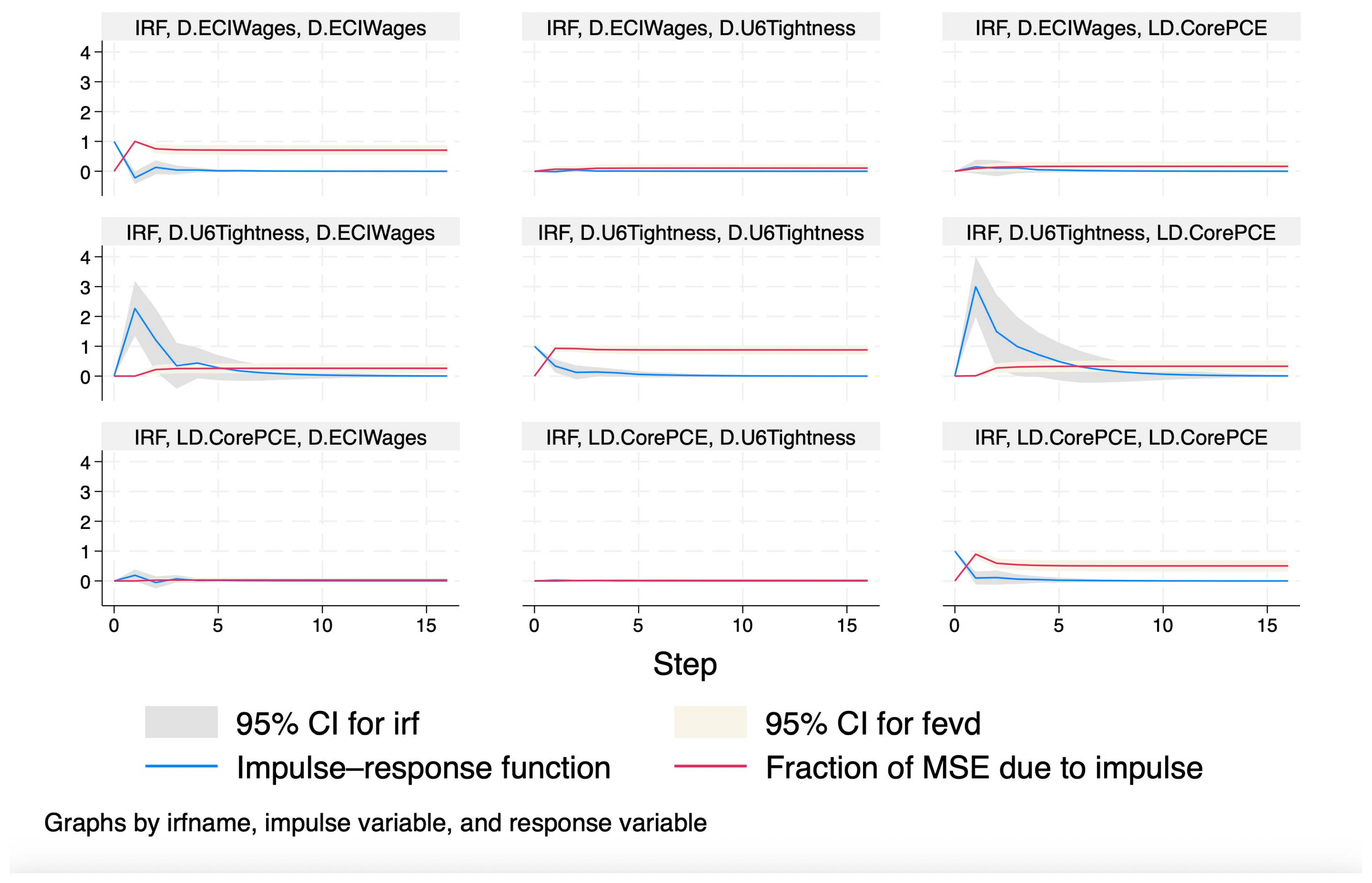
Figure 2 below displays the Impulse Response Functions for the Vector Error Correction Model estimated in Table 9 and Table 10. They highlight the impact of shocks on U6 Tightness on the lagged Core PCE and the Employment Cost Index. There is a sizable impact of a shock to U6 Tightness on the Employment Cost Index, and the impact persists for several quarters before it dissipates. There is also a sizable impact of a shock to U6 Tightness on the lag of Core PCE. This impact also persists for several quarters before it too dissipates, suggesting that U6 Tightness influences both the Employment Cost Index and lagged Core PCE. This dual effect confirms OLS estimates of a wage–Phillips curve relationship, but it also suggests that there still exists a relationship between the labor market and overall inflation, as evidenced by the impact of a shock on U6 Tightness on the lag of Core PCE.

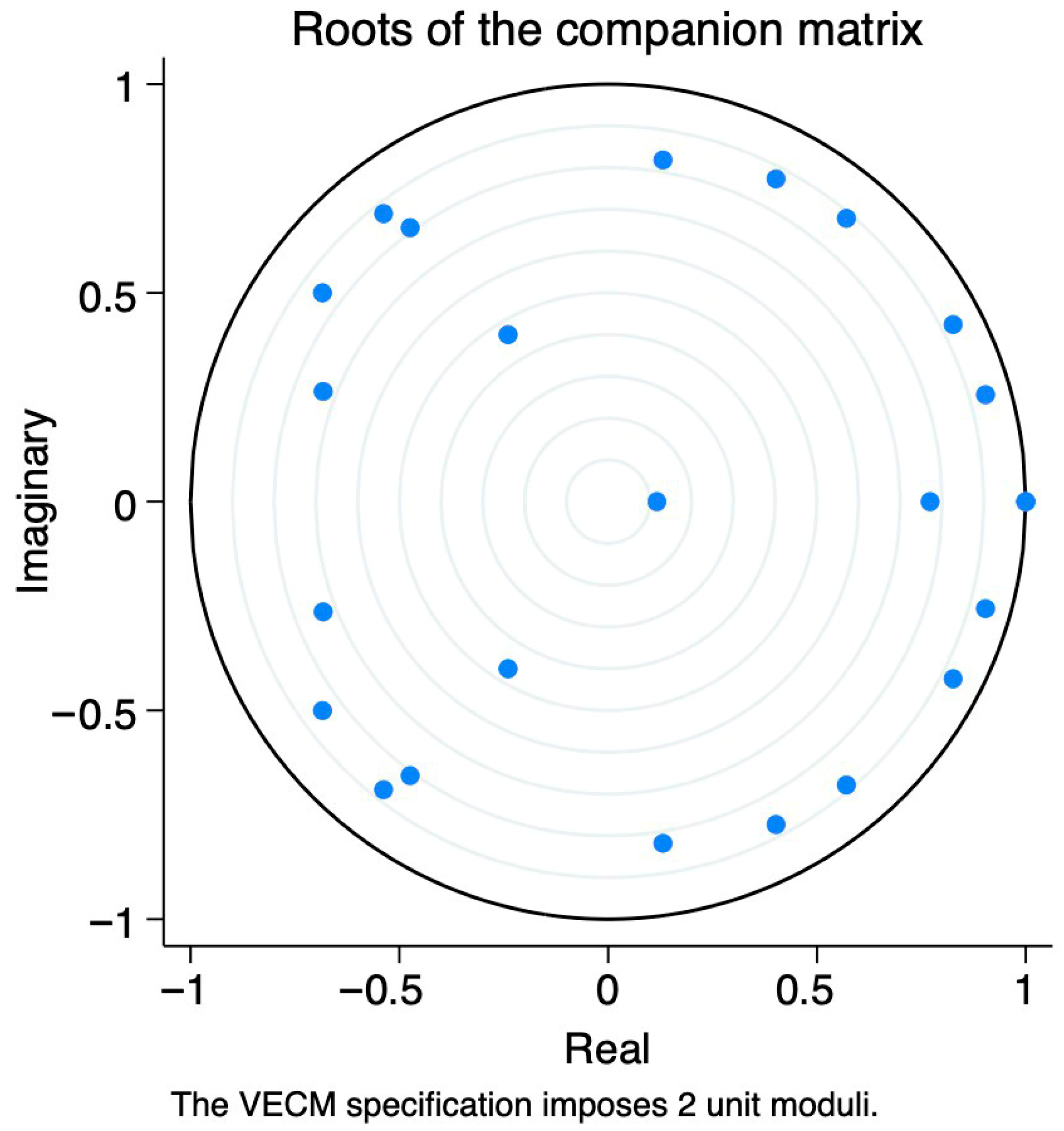
After running the Vector Error Correction Model and displaying the results of the variance decomposition and the Impulse Response Functions, I decided to assess its stability. I was able to determine that the model was in fact stable, as all the roots lie within the unit circle, as demonstrated by Figure 3 below. Furthermore, the Durbin–Watson test was performed to determine whether there was serial correlation in the residuals of the model at the appropriate delay. The results confirmed that there is in fact no serial correlation at eight lags, which is what the VAR Lag Order Selection Criteria suggested, because the Durbin–Watson Test statistic was very close to 2 (1.942). A value of two indicates that there is no significant autocorrelation.

5. Discussion

The results in this paper suggest that the comprehensive model in Atesoglu (1997) is preferred to the Atesoglu (1980) basic wage-cost markup equations for the period 2002 to 2024. Despite this, the model is not robust due to the sign and magnitude of the coefficient on unit labor costs in the wage-cost markup equation in Table 4. The question therefore is, why have the structural parameters in the aggregate demand–augmented wage-cost markup model changed? Data are often revised over time, and this can have an impact on the time-series elements of the data, such as stationarity. In addition, the US economy itself has changed over time, which can undoubtedly have an impact on the structural parameters of the model. I will briefly highlight some of the factors that contribute to the change in the structure of the model.

Post Keynesians have argued that we have limited information about the world. Lavoie (2009) stresses that “the world is non-ergodic, meaning that the averages and the fluctuations observed in the past will not necessarily be observed in different time periods” (Lavoie, 2009). In addition, Post Keynesians emphasize the role of path dependence. Setterfield (2015) explains that “a dynamical system displays path dependence if earlier states of the system affect later ones, including (but not limited to) anything that can be construed as a “long run” or “final” outcome of the system” (Setterfield, 2015).

The updated wage-cost markup equation in Table 4 yields significant results; however, the coefficients are considerably smaller than the results found in Atesoglu (1997). Many Post Keynesians emphasize Kaleckican markup pricing theory, where firms charge a markup over unit labor costs and operate in oligopolistic markets with excess capacity. In addition, marginal costs are constant up to full capacity. Firms can resist increasing prices by reducing profit margins and, therefore, the markup, to maintain goodwill with customers. Furthermore, excess capacity allows firms to ramp up production in response to temporary surges in demand rather than raising prices. Bobeica et al. (2021) argue that factors such as anchored inflation expectations, the impact of globalization and import competition, technological advancement, the decline in union power, and the structural shift toward a service-oriented economy have collectively weakened the historical link between unit labor costs and inflation.

It is interesting to note that the COVID-19 dummy variable is significant at five percent and quite large (0.289). Although beyond the scope of this paper, it suggests that supply shocks such as the COVID-19 pandemic can have significant impacts on inflation. This result seems to support the research by Weber and Wasner (2023), who argue that firms with markup power can hike prices during times of emergency. The authors suggest that this can materialize if firms expect their competitors to also raise their prices. “This requires an implicit agreement which can be coordinated by sector-wide cost shocks and supply bottlenecks” (Weber & Wasner, 2023).

The updated wage growth equation in Table 2 yields significant results and the coefficient on U6 Tightness was larger (1.330) for the period 2002 to 2024 than the coefficient on unemployment (0.355) for the Atesoglu (1997) model for the period 1974 to 1993. The reason why the Atesoglu (1997) equation does not hold is the fact that the U3 unemployment rate13 does not adequately capture changes in slack in the labor market. Other measures, such as U6 Tightness, are a more comprehensive measure of labor market slack. The results of this paper support the existence of a substantial wage–Phillips curve relationship. The problem is that although tight labor markets may correspond with higher wages, the pass through to prices may be less straightforward. There may exist a wage–Phillips curve; however, the relationship between the labor market and broader inflation measures may be more complex. The Conflicting Claims Model14 (Rowthorn, 1977; Lavoie, 1992; Setterfield, 2006) highlighted earlier in this paper may offer an explanation for this complexity and the flattening of the Phillips curve.

Summa and Serrano (2018) stress that in Brazil “the strengthening of the bargaining power of workers and rising real wages since 2006, combined with continuous nominal ex-change rate depreciation after mid-2011, increased distributive conflicts and are ultimately behind the recent shift toward austerity” (Summa & Serrano, 2018). The work of Summa and Serrano is notable because austerity measures were passed in the United States during the early recovery from the Great Recession, and the labor share of income (which has experienced a secular decline) remained at historically low levels throughout the recovery. It is worth noting that there is empirical support for a connection between a low interest rate environment (as in the case of recovery from the Great Recession), and a flat Phillips curve; however, the evidence for a flat Phillips curve when interest rates are high is not entirely clear.

Quite a lot of research has been devoted to the flattening of the Phillips curve. Gross and Semmler (2019) emphasize a non-linear or convex Phillips curve that is flat as firms operate at below capacity during times of economic weakness, but rises as firms operate above capacity during economic booms. Another convincing theory is the aforementioned Conflicting Claims Model as described in Setterfield (2006), which emphasizes the opposing effects of a low unemployment rate, which raises bargaining power, wage, growth, and the inflation rate in equilibrium with a decline in union density of the same magnitude, which lowers bargaining power, wage growth, and the inflation rate in equilibrium.

A recent paper by Ratner and Sim (2022) also emphasizes the role of bargaining power in describing the flattening of the Phillips curve. The authors suggest that structural factors related to the fall in union density described in Grossman and Oberfield (2021) have led to a decrease in the bargaining power of workers. The authors incorporate a conflict theory of inflation that leaves virtually no role for monetary policy to affect inflation. “We show that a nearly ninety percent reduction in inflation volatility is possible even without any changes in monetary policy when the economy transitions from equal shares of power between workers and firms to a new balance in which firms dominate” (Ratner & Sim, 2022). It is worth noting that there are some serious critiques of the authors’ model due to its flawed interpretation of Kalecki, as stressed in Matamoros Romero and Seccareccia (2022).

The results of Ratner and Sim (2022) imply that monetary policy has very little influence on the Phillips curve. This is in stark contrast with a Post Keynesian view of conflict inflation, as emphasized in Setterfield (2006). Similarly, Setterfield and Herdelin (2026) develop a model of the Goodwin pattern and the central bank where monetary policy via a Taylor rule intervenes when there are variations to the wage share and real activity. The model incorporates asymmetry in the central bank’s reaction function, which can demonstrate “downward trends in the wage share accompanying the distributive cycles associated with the Goodwin pattern. In this way, the model integrates trend and cycle in a manner that captures both the Goodwin pattern and the secular decline in the wage share of income characteristic of advanced capitalist economies in recent decades” (Setterfield & Herdelin, 2026, Manuscript in preparation). The model therefore suggests that the central bank via monetary policy using a Taylor rule has a pronounced influence over the flattening of the Phillips curve.

This is supported by Kappes (2023), who suggests that “There is evidence that increases in interest rates have statistically significant effects on income distribution, whereas the effects of reductions in interest rates are not statistically different from zero. This empirical finding goes against the conventional view that the distributional effects of interest rate changes are temporary and likely to net out over the business cycle” (Kappes, 2023).

6. Conclusions

In this paper, I investigate the causes of inflation from a Post Keynesian perspective using quarterly data for the period 2002 to 2024 and contrasts earlier work done on the subject by Atesoglu (1980, 1997). I found that the Post Keynesian wage growth model, using the implicit price deflator and the headline unemployment rate, did not produce significant results; however, an updated model featuring alternative measures of labor market slack and inflation produces a model with significant results and an improved fit using model selection criteria such as the Akaike Information Criterion (AIC) and the Schwarz Bayesian Criterion (SBC).

Although the updated model produced significant results and a better overall fit in terms of model performance, the magnitude of the coefficients on unit labor costs, unemployment, and inflation for the updated wage-cost markup model decreased substantially for the period 2002 to 2024. In addition, the sign on the coefficient for unit labor costs in the wage-cost markup model was negative, which is not a typical Post Keynesian result. A more predictable outcome was that the coefficient on the COVID-19 dummy variable was large and significant, suggesting that the pandemic had a sizable impact on the inflation rate in the US. Finally, the updated model supported the role of aggregate demand, as evidenced by the relatively large and significant coefficient on output.

Robustness testing of the expanded wage-cost markup model, utilizing Prais–Winsten regression to address autocorrelation, demonstrates that while the unit labor cost coefficient remains positive, supporting the results found in the original Atesoglu wage-cost markup equation, it becomes statistically insignificant when accounting for energy and import costs. The model in Table 5 outperforms the Table 4 specification, indicating a structural shift where external factors, rather than a simple markup over unit labor costs, are the primary drivers of inflation.

The updated wage growth equation displayed significant results; however, there were questions regarding endogeneity as well as cointegration. The model was extended using a Vector Error Correction Model (VECM), which deals with potential endogeneity and the presence of cointegration, which was confirmed via the Engle–Granger test in Table 7. The Vector Error Correction Model confirmed the robustness of the results of the updated wage growth equation in Table 2, where a shock to U6 Tightness has large and persistent effects on the Employment Cost Index. In addition, the variance decomposition and Impulse Response Functions demonstrate that a shock to U6 Tightness also has large and persistent effects on the lag of Core PCE as well.

Section 5 highlighted some key explanations for the weakening of the coefficients in the comprehensive Post Keynesian model of inflation. First, it was emphasized that the data are revised, and the properties of time-series data can change over time even absent revisions in the data. This is why Post Keynesians stress that the world is non-ergodic, where economic relationships in the past may not be likely to hold in the future. Section 5 also highlighted research that emphasizes the role of the central bank in the weakening of the relationship between unemployment and inflation that contributed to the flattening of the Phillips curve. Current research by Setterfield and Herdelin (2026) investigates how a central bank such as the Fed, via a reaction function such as the Taylor rule responding to variations in the wage share, produces a Goodwin pattern, but also based on an asymmetric reaction function, the Fed can negatively influence the trend in the wage share, which can explain in part the weak relationship between measures of labor market slack and the inflation rate.