Abstract
This article presents a transparent and replicable framework to assess the net worth of public pension systems within the broader context of fiscal sustainability and public sector balance sheets. Using Spain as a case study, it transforms Eurostat’s Table 29 data into an actuarial balance sheet and income statement, applying the Swedish open group (SOG) approach. The analysis shows that Spain’s pension system faces a significant funding shortfall, with assets covering only 72% of its liabilities. The proposed method enhances fiscal transparency and provides policymakers with a practical tool to evaluate and improve long-term pension sustainability across different institutional contexts.
1. Introduction
Extant literature underscores that traditional fiscal indicators—such as the annual ratio of revenues to expenditures or aggregate government debt—are insufficient to capture the complete picture of public financial health, as they overlook changes in government assets (Easterday & Eaton, 2012). Public sector accounting practices are often less stringent than those applied to private sector defined benefit schemes, and conventional frameworks for managing public finances fall short in ensuring long-term sustainability, efficient resource management, and intergenerational equity. Many governments either refrain from producing full financial statements or release them too late to be of practical use, often omitting crucial details on the value of public assets. Only a handful of countries—New Zealand being a notable example (Ball et al., 2024)—prioritise the balance sheet as the central element in fiscal decision-making.
Researchers including Milesi-Ferretti and Moriyama (2006), the IMF (2014), Levy Yeyati and Sturzenegger (2023), and Ball et al. (2024) advocate adopting a balance sheet approach (BSA), arguing that public sector balance sheets yield a comprehensive view of a state’s financial standing by considering assets alongside liabilities. Such an approach facilitates effective management, revenue generation, and risk mitigation. Fiscal stress tests based on balance sheet metrics offer a robust measure of fiscal resilience, with a focus on net worth proving crucial for sound governance (Ball et al., 2024). Plummer and Patton (2015) demonstrate that financial statements can expose long-term fiscal imbalances, reinforcing the rationale for applying a similar framework to public pension obligations.
Public pension entitlements are a pivotal aspect of public finances. Our analysis focuses on the actuarial balance sheet (ABS), particularly net worth, which summarises the difference between a pension system’s assets and liabilities, thereby reflecting its overall financial position. While numerous pension statistics exist—as seen in social protection data—these measures typically capture annual flows (such as contributions and benefits disbursed) rather than a forward-looking assessment of future pension payments. Historically, pension liabilities have been treated as “out of sight, out of mind” because governments have been reluctant to recognise them on balance sheets due to the potential negative impact on their reported financial positions (PriceWaterhouseCoopers, 2014).
Eurostat, along with EU Member States and EFTA countries, has sought to address this gap by publishing a snapshot of pension scheme liabilities—referred to as Table 29 of supplementary pensions. This data is submitted triennially: the initial transmission in December 2017 covered 2015 data, followed by the second wave in December 2020 for 2018 liabilities, with the third wave on 2021 data released recently (Eurostat, 2024a, 2024b). Table 29 disaggregates social insurance pension entitlements accrued by the end of a reporting period for current affiliates and pensioners, broken down by scheme type, institutional sector, manager category, recording method, and accounting classification. This classification distinguishes between the stock of pension entitlements—recorded at both the beginning and end of the period—and the flows that drive changes in these entitlements, such as social contributions, benefit payments, revaluations, transfers, and legislative reforms.
The Table 29 pension reporting exercise relies on the accrued-to-date pension liability (ADL) method, which aligns with the closed-group approach. Under this method, a plan’s liabilities equal the present value of all anticipated future benefits to pensioners and the accrued rights of current affiliates (this analysis can be provided by the author upon request). These accrued rights, analogous to a termination reserve in private or occupational schemes, represent both past social contributions and the remaining pension entitlements, thereby reflecting the resources needed to liquidate a social security scheme while meeting all prior obligations (Kaier & Müller, 2015; Wiener & Stokoe, 2018).
Although the Table 29 methodology provides pertinent data for pension systems financed by full advance funding, it does not suffice to assess the financial sustainability of social security schemes—typically financed on a pay-as-you-go or partially funded basis. In contrast, the actuarial balance sheet (ABS) and its associated income statement (IS) are better suited to a wide variety of schemes (Boado-Penas et al., 2008; Ventura-Marco & Vidal-Meliá, 2014; Vidal-Meliá, 2014; Pérez-Salamero González et al., 2017; Metzger, 2018; Vidal-Meliá et al., 2018; Billig & Ménard, 2018; Metzger, 2019; Garvey et al., 2021, 2023; TSPS, 2023). This approach rectifies the primary limitation of Table 29, which—in considering liabilities alone—fails to indicate solvency or sustainability, leaving pensioners and contributors without crucial information on the probability of receiving their future benefits.
However, unlike the case of private corporations, where solvency is defined in terms of accrued liabilities and existing assets, a meaningful actuarial balance sheet for a pay-as-you-go system must also include the present value of future contributions on the asset side. Following the Swedish open group approach (SOG), we estimate these contribution assets through turnover duration, which ensures that the solvency measure is aligned with the renewable nature of social security schemes.
The actuarial balance sheet (ABS) details a pension system’s obligations to contributors and pensioners at a specific date, supported by pertinent assets—particularly those from contributions. Conversely, the income statement (IS) summarises the pension plan’s financial performance over a period, detailing gains, expenses, losses, and the resultant net profit or loss.
This paper makes a significant contribution to pension management by advocating for a transparent methodology that reflects the true net worth of social security systems—moving beyond traditional opaque approaches. It outlines a detailed procedure for converting Table 29 data into an actuarial balance sheet (ABS) and income statement (IS), updating the Spanish social security system’s results. This model aids policymakers and public finance economists in better understanding and implementing the ABS/IS approach. Furthermore, the paper discusses policy implications by comparing Spain’s pension solvency internationally and exploring measures to restore it. Emphasising transparency and simplicity, it argues that net worth—which integrates all assets and liabilities—provides a more robust indicator of sustainability, solvency, and resilience than conventional fiscal metrics.
Beyond Spain, the framework can be applied to any country with Table 29 disclosures, enabling routine, comparable ABS-based solvency assessments across the EU.
The paper is structured as follows. Following this introduction, Section 2 explains the methodology and data collection in two parts: the first outlines a nine-step process to convert Table 29 into an ABS and its corresponding IS; the second presents the necessary data. Section 3 updates Garvey et al.’s (2023) results for the Spanish social security system using the latest Table 29 data, while Section 4 discusses the policy implications of transforming Table 29 into an ABS. The paper concludes with final remarks and references. This analysis, including the calculations for estimating accrued pension entitlements and the formulas used for the ABS and IS, is presented in the Technical Appendix A and Appendix B.
2. Methodology and Data
Methodology. Supplementary Table 29 records positions and flows associated with pension obligations for all social insurance schemes, detailing both the schemes’ liabilities and the counterpart entitlements held by households.
This paper applies the methodology developed by Garvey et al. (2023) to transform Table 29 into an actuarial balance sheet (ABS) and generate the related income statement (IS).
Figure 1 summarises Garvey et al.’s (2023) method through a stock and flow model. Stock at t − 1: pension entitlements, other liabilities, and the system’s assets at the beginning of the period. Stock at t: pension entitlements, other liabilities, and the system’s assets at the end of the period, along with transactions and other flows between t − 1 and t. These flows, necessary for compiling the income statement, include all economic transactions that change the opening and closing stocks. Figure 1 shows the system’s assets and liabilities on two consecutive valuation dates, along with their changes. The main formulae for converting Table 29 into an ABS and its associated IS are presented in the Technical Appendix B.
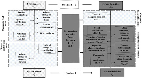
Figure 1.
The system’s assets and liabilities on two consecutive valuation dates and their changes. Source: Own elaboration based on Garvey et al. (2023).
The reconciliation between opening and closing stocks considers all transactions and flows during the period. In Figure 1, shaded areas represent information derived from Table 29, regardless of recalculations, while unshaded areas indicate new data required for the ABS.
Accrual accounting is more appropriate than cash-based methods for promoting intergenerational fairness and sustainability. It enables pension systems to measure financial positions more accurately by fully recognising assets and liabilities, offering a clearer view of financial health—crucial for sound decision-making (Ball et al., 2024).
As shown in Figure 1, changes in net worth can be classified into four key components: (1) fund/financial asset variation, (2) contribution asset variation, (3) pension liability variation, and (4) change in financial liabilities. The ABS relies on net worth—positive when assets exceed liabilities. In public pension systems, negative net worth signals insolvency. As Ball et al. (2024) argue, net worth is central to the ABS, reflecting all assets and liabilities, better capturing sustainability, solvency, and resilience. Davidyan and Waymire (2018) show that stronger adherence to accounting standards correlates with improved pension funding and greater transparency. Changes in net worth can be broken down into (1) the change in the fund/financial asset, (2) the change in the contribution asset, (3) the change in pension liability, and (4) the change in financial liabilities.
In this paper, contribution asset denotes the present value of future contribution inflows attributable to current contributors in a PAYG scheme. In the Swedish open-group formulation, it is operationally estimated by taking the current contribution flow and applying the turnover duration, understood as the average time between a unit contribution and the corresponding pension disbursement. Recognising the contribution asset alongside accrued entitlements is essential for a meaningful solvency measure in PAYG systems (see the Technical Appendix B for derivations and notation).
We adopt the SOG approach: liabilities are accrued pension entitlements at the valuation date (as in Table 29), while assets include the contribution asset, computed without explicit projections and included as current contribution revenue × turnover duration (TD). Under unchanged rules and the prevailing economic-demographic conditions at the valuation date, this procedure is operationally equivalent to a perpetual horizon, with the State acting as the ultimate guarantor of PAYG obligations.
The structure and key figures of the supplementary table are used to determine pension liabilities at two valuation dates and their variation. This leads to nine steps for deriving the ABS, IS, and solvency metrics from Table 29:
- Assessment of Assumptions: Pension liabilities at a specific date are analysed to verify that the assumptions applied are appropriate, unbiased, consistent, and based on verifiable data. This requires comparing reliable historical information—such as changes in GDP, wages, contribution income, and pension revaluation—with the assumptions used.
- Adjustments and Exclusions: Adjustments or exclusions are applied to the valuation of pension liabilities for contributors and pensioners, mainly due to missing data or irrelevance of certain liabilities. Key assumptions—such as the discount rate and indexation rate—are updated as needed. As Gronchi et al. (2023) highlight, failing to regularly update such assumptions can distort actuarial fairness and threaten long-term solvency, especially in countries lacking cohort-sensitive adjustments.
- Inclusion of Financial Liabilities: Pension systems often borrow to meet benefit payments, generating financial liabilities from accumulated treasury deficits. Although Table 29 does not report these, they should be included in the ABS as real obligations of the pension system.
- Safeguard Mechanisms: The final component on the liability side is whether the pension system includes mechanisms to safeguard benefits, as many developed countries do. This information is often found in state budgets, particularly under sponsor contributions for supplementary benefits (SBs).
- Valuation of Contribution Asset: With the liability side complete, the next step is to value the system’s contribution asset, estimated by multiplying current contribution revenue by the expected time between paying contributions and receiving benefits—known as turnover duration.
- Reserve Fund (Buffer): The asset side may include a buffer or reserve fund, representing the stock of financial assets held by the system. Its purpose is to offset temporary mismatches between contributions and benefit payments, and it may originate from treasury surpluses or extraordinary sponsor contributions.
- Calculation of Net Worth: The scheme’s net worth is calculated. A stronger ABS—i.e., higher net worth—provides advantages such as greater flexibility during crises, faster recovery after shocks, and more certainty regarding benefit payment capacity, while helping to avoid shifting fiscal adjustment burdens onto future generations.
- Compilation of the Income Statement: The income statement is compiled, reflecting changes in the scheme’s net worth. Under a present value model, assets and liabilities are valued at the reporting date, and periodic changes are recorded as income or expenses.
- Solvency Indicators: The system’s main solvency indicators are then shown: the solvency ratio (), a common measure used to assess the system’s financial health, and the required growth rate .
Once the ABS and IS are compiled, stakeholders gain valuable insights—not only the quantified value of public pension promises but also, crucially, a reliable estimate of the likelihood of receiving these future benefits.
Discounting convention (no-projection design). Present-value figures use a long-run nominal rate given by the 27-year geometric average of real GDP growth and CPI, ending in year t – 2. This backward-looking, verifiable parameter aligns with the system’s maturation (TD) and avoids projection-driven volatility. Unlike the UK practice of tying public-service pension rates to expected GDP growth (O’Brien & Zaranko, 2023), our parameter choice is auditable and stable, reflecting system maturation while avoiding projection-based inputs.
Plain-language note on discount and growth. Our discount rate is based on realised—not forecast—macro data. Concretely, we take a long-run geometric average of real GDP growth over a window that matches the system’s turnover duration (≈27 years) and combine it with the long-run CPI average to obtain a nominal rate. Using a backward-looking window aligned with maturity keeps the valuation auditable and stable year-to-year and avoids the optimism and volatility of long-horizon projections. Intuitively, it answers: “Given today’s rules and demographics, what has the economy actually delivered on average over one full contributor-to-pensioner cycle?” That figure then discounts future cash flows consistently with the open-group nature of PAYG. Illustration (2021): the 27-year real GDP average is ≈1.88%, and together with the long-run CPI, it implies a nominal rate of ≈3.91% used throughout our ABS/IS.
No-projection rationale (Swedish open-group). Consistent with the SOG principle of valuing only verifiable facts at the valuation date, we deliberately eschew explicit macro-demographic projections. Long-horizon forecasts are prone to sizeable and systematic errors: accuracy deteriorates quickly as the horizon extends beyond the very short term (Kammer, 2023; Celasun et al., 2022), and forecast errors arise from information gaps, structural volatility, shocks, and forecaster bias/capacity (Gatti et al., 2024). Empirically, GDP-growth forecasts tend to be upward-biased, especially one year ahead and beyond (Timmermann, 2007; Morikawa, 2022). In contrast, our parameter choices are backward-looking and auditable.
The transformation from Eurostat’s Table 29 to the actuarial balance sheet (ABS) is transparent and replicable; Appendix A details the estimation of Table 29 accrued-to-date liabilities, and Appendix B compiles the main formulas used to construct the ABS and its income statement.
Our solvency metric differs from generational accounting (GA), which assesses very long-term sustainability under projected demographics by computing lifetime net tax rates for each cohort and for future generations (Auerbach et al., 1992, 1994; Kotlikoff & Raffelhüschen, 1999). While influential, GA is projection-dependent and abstracts from many institutional details of pension systems (Holzmann et al., 2001); critics also note issues of complexity, logic, and validity (Ruffing et al., 2014). By contrast, our SOG implementation evaluates solvency at the valuation date under a mature-state assumption using verifiable contemporaneous data and no explicit macro-demographic projections; with annual updates, each interval can be read as a transitory steady state (Lee, 2006), consistent with Swedish practice (TSPS, 2022).
Data. We begin with pension obligation data from the Instituto Nacional de Estadística (INE) for 2015, 2018, and 2021, as reported in Table 29.
Table 1 displays data for the social security system, which accounts for roughly 91% of total pension liabilities in 2015, 2018, and 2021. This includes retirement, survivor, family, and disability pensions. The Clases Pasivas scheme is excluded due to insufficient data for estimating its contribution asset. Rows with zero values across all columns were omitted.

Table 1.
Pension table (base scenario) for 2015, 2018, and 2021 social security, Spain. Unit: EUR million.
Figure 2 illustrates the evolution of unfunded pension entitlements (social security and civil servants) in selected EU countries for 2015, 2018, and 2021. For Spain, Figure 2 aggregates the social security scheme and the government employer (civil service) pension scheme, whereas Table 1 reports only the social security scheme. Consequently, the percent-of-GDP values for Spain in Figure 2 are higher and are not directly comparable to the last row of Table 1. In 2021, Spain topped the ranking, surpassing Austria, Italy, France, and Portugal. From 2015 to 2021, Spain’s pension liabilities rose by 74% of GDP—the highest increase in the EU. The second-highest, Hungary, registered a 47% rise over the same period.
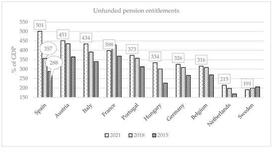
Figure 2.
Evolution of the unfunded pension entitlements in the closing balance sheet. Source: Own elaboration based on https://ec.europa.eu/eurostat/databrowser/view/nasa_10_pens1/default/table?lang=en&category=na10.nasa_10_pens (accessed on 12 May 2025).
The sharp rise in Spanish pension entitlements between 2018 and 2021 is mainly due to a revised assumption on pension indexation, as shown in Table 2 below.
Table 2.
Main assumptions in % for the period 2014–2021.
Data on GDP growth (datosmacro.com), historical pension indexation, financial liabilities, contributions, and disbursements (MTES, 2024a, 2024b) complement this analysis. The MISSM (2022) reports the Reserve Fund’s status for 2014–2021. Although the system borrows to pay benefits, the fund nominally persists for political reasons. As of 31 December 2021, its actual balance stood at –79,874 million euros—the so-called “pension piggy bank” is essentially empty. As Väänänen (2021) notes, the long-term effectiveness of reserve funds depends not only on their existence but also on their governance, legal constraints, and integration into the pension system’s financial framework. His comparative study of Sweden’s AP4 and Finland’s Keva shows how legal autonomy and investment mandates shape a fund’s resilience and its capacity to contribute meaningfully to sustainability—features absent in Spain’s politically exposed and now largely depleted reserve fund.
Turnover duration (TD) is calculated using data from the Continuous Sample of Working Lives (MCVL), which compiles anonymised administrative microdata from Spanish social security records. This sample provides detailed individual-level work histories, forming the empirical foundation for estimating contribution asset duration.
As noted in the methodology, turnover duration (TD) is key to estimating the contribution asset. For Spain, TDs remained stable from 2014 to 2021, consistently rounding to 27 years. This stability benefits both the valuation of the contribution asset and the determination of the discount rate in the actuarial calculation of pension entitlements.
Considering only the retirement contingency (TDr), the TD would be 1.5 to 2 years higher—comparable to the Swedish system (TDsw), which also focuses solely on retirement (TSPS, 2020, 2021, 2022, 2023).
Essentially, the inverse of turnover duration functions as the discount rate for calculating the present value of a perpetual income equivalent to one year of contribution revenue.
The TD for disability (TDd) is lower than for retirement, as beneficiaries are reclassified upon reaching retirement age. The survival contingency TD (TDsr) remains stable, consistently rounding to 29 years throughout the observed period.
3. Results
The results in this section draw on the previously described methodology, the data outlined below, and a revision of certain basic assumptions that appear clearly biased when assessed against observable data and verifiable facts in the ABS and IS construction.
Best practice in DB scheme valuations defines unbiased assumptions as neither imprudent nor overly conservative. Assumptions should be mutually compatible, reflecting economic relationships between inflation, salary growth, and discount rates. SS schemes should assess defined benefit obligations based on expected future benefit changes. The future indexing rate is typically derived from historical or reliable evidence, often assuming pensions in payment will follow general price or salary trends.
Together with dynamic mortality tables, the key assumptions used by INE to calculate pension entitlements at year-end 2015, 2018, and 2021 appear in Table 2.
Using general population mortality tables in Spain may underestimate pension liabilities, as retirees at age 65 live about three years longer than the general population (Pérez-Salamero González et al., 2022; Vidal-Meliá et al., 2023). Eurostat (2020) recommends using scheme-specific mortality data when discrepancies exist. For disability and reclassified retirement pensions, INE (2023) applied tables estimated by the Ministry of Labour, but we could not locate these sources to verify their validity.
As shown in Table 2, Table 29 for Spain used a nominal discount rate of 5% for 2014–2015 and 4% for 2017–2021, with inflation fixed at 2% and pension indexation at 0.25% during 2014–2018. However, this indexation assumption diverged from actual inflation, violating the verifiability principle. As previously noted by Garvey et al. (2023), this led to an underestimation of pension liabilities for the 2014–2018 period. INE’s 2023 report revised its assumption on pension indexation, now aligning revaluation with the expected 2% inflation rate—a notable departure from the previous, significantly lower, indexation hypothesis. The best estimate of the real discount rate (1.88% in 2021; 1.73% in 2020) differs from the 1.96% applied by INE (2023). As previously defined in the Methodology section, we use the real average annual GDP growth over the past 27 years, consistent with the TD. This approach offers transparency and stability and reduces solvency indicator volatility. Eurostat (2020) supports applying a stable discount rate to avoid distortions from frequent assumption changes.
Table 3 extends Spain’s Table 29, presenting the 2021 income statement and simplified ABS. Table 4 summarises the key indicators and data derived from Table 3.
Table 3.
The ABS and IS for the 2021 social security scheme, Spain. Unit: EUR million.
Table 4.
Solvency/sustainability indicators for the years for which data are available.
The income statement for 2021 reports substantial actuarial profits: EUR 159,589 million (13.06% of GDP; see Table 4, row 3). This profit reflects the difference between asset and liability increases—EUR 205,578 million and EUR 45,989 million, respectively. The key driver is the “Changes in entitlements due to revaluations and other” item, which includes the effect of raising the discount rate from 3.77% to 3.91%. This adjustment alone (–EUR 172,706 million) significantly reduced the liability increase, explaining the system’s positive actuarial result in 2021.
The system’s asset growth in 2021, totalling EUR 205,578 million, stems from contributions, including those from the state. However, its financial assets—the Reserve Fund—remained unchanged. As of 31 December 2021, the fund was fully deposited at the Bank of Spain, with no investments in financial instruments.
Despite the actuarial gains in 2021, the opening ABS (1 January) revealed a large shortfall of EUR 1,743,333 million, with a solvency ratio of 0.6951 (Table 4, Row 2). The closing ABS (31 December) incorporates the year’s transactions, including actuarial profits, resulting in a modest improvement to a solvency ratio of 0.7252. At present, only 72.52% of liabilities are covered by assets, leaving 27.48% unfunded. This means the sponsor must eventually allocate additional resources, or some promised benefits—particularly to younger contributors—risk being only partially fulfilled.
It is important to note that the solvency indicator includes transfers made by the state to the system as part of the public contribution asset. However, if these transfers are excluded from the calculations, the primary solvency index is obtained (Row 1 in Table 4). This presents a more accurate depiction of the sustainability of the system, and its values for 2021 (0.5564) and 2020 (0.5262) show the severity of the problem, especially considering that it started from a value of 0.7505 in 2014.
Row 3 reports actuarial results—the year-over-year change in net worth as a share of GDP (positive = gains, negative = losses)—while Row 4 reports the net liability (accumulated shortfall) as a share of GDP (liabilities minus assets), i.e., the gap depicted in Figure 3.
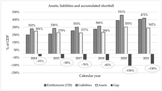
Figure 3.
Evolution of total assets, total liabilities, and the accumulated shortfall (“gap”) as % of GDP (2014–2021). Source: Own elaboration based on Garvey et al. (2023).
Figure 3 shows the evolution of assets, liabilities, and the accumulated deficit as a share of GDP. Spain’s pension system faces a growing deficit, as liabilities rose at 7.73% annually, outpacing assets (4.35%). Solvency recovery requires reversing this trend, yet recent years have seen the opposite.
Accumulated liabilities relative to GDP rose sharply between 2014 and 2021—from 3.32 to 4.72 times GDP—despite the reported actuarial gains in 2021.
In the latest year, actuarial profits are positive, yet the net liability—the gap shown in Figure 3—remains sizeable.
Figure 3 indicates a 2021 net liability of 130% of GDP—4.16 times higher than in 2014—placing the Spanish social security system in a “critical and declining” condition.
Finally, the required growth rate (), which actuarially matches the pension system’s liabilities with its assets at the valuation date, presents an extraordinarily high value of 3.20% (row 6 in Table 4) compared to the real discount rate used to calculate pension liabilities in 2021, which was 1.88% (Table 2). In other words, the discount rate (the future growth rate, and ceteris paribus) that should be applied is 70% (1.32% gap in , row 7 in Table 4) higher in real terms than the average rate recorded over the last 27 years. Without sponsor transfers (Table 4, row 9), the growth gap rises to 2.14%, implying the Spanish economy must grow at 4.02% annually in real terms—114% above the recent average, a scenario deemed highly improbable.
Table 4 also reports the duration of the pension liability, which rose from 16.32 years in 2014 to 20.99 in 2021, reflecting increased sensitivity to discount rate changes. Convexity remained positive throughout, meaning liabilities rise more from falling rates than they fall from rising ones. Spain’s duration values in 2015, 2018, and 2021 are comparable to the European average, as are its positive convexity values.
As the solvency indicators are dependent on the assumptions made, Table 5 analyses the potential impact on the system’s solvency indicators at the end of 2021 if there were changes in both the relative value of pensions in payment (%) and the discount rate used (). The shaded cells show the value for our best estimate assumption (base scenario).
Table 5.
Sensitivity analysis for the solvency indicators at the end of 2021.
In the case of the basic solvency indicator, values equal to or above unity would only occur in scenarios of exceptionally high future economic growth and below-expected inflation revaluation of pensions in payment. However, such scenarios are unlikely to occur in practice.
With regard to the primary solvency indicator (), it was found that in only one of the explored cases would the indicator reach a value above unity. This was contingent upon the assumption of a highly optimistic economic growth scenario and the indexation of pensions in payment at a rate far below the anticipated rate of inflation (RPI).
AIReF (2023) projects average real GDP growth of 1.3% and nominal growth of 3.3% between 2027 and 2070—well below the 3.91% best estimate used for 2021 in our model.
The basic and primary solvency indicators would be 0.6443 and 0.4943, respectively, under the AIReF scenario.
4. Discussion
Timely and regular information is crucial for transparency and accountability. For instance, Table 29 for the year ended 31 December 2021 was published in December 2023. However, by the beginning of 2024, more than two years had passed since the last supplementary table on pension entitlements had been published. To make matters worse, Table 29 is only compiled every three years for data relating to year . This indicates that the EU is not using Table 29 for any significant decision-making purposes. In essence, there is considerable doubt as to whether the EU is treating this matter with the seriousness it deserves. For context, the following quotation predates Eurostat’s Table 29 and addresses the broader lack of transparent reporting on unfunded social security liabilities.
The initial thought is a statement by Hoogervorst (2012), Chairman of the International Accounting Standards Board (IASB), on 20 June 2012, addressing the International Association for Accounting Education and Research (IAAER) conference in Amsterdam: “Around the world, governments give very incomplete information about the huge, unfunded social security liabilities they have incurred. Many executives in the private sector would end up in jail if they reported like Ministers of Finance, and rightly so”.
This remark concerns transparency and solvency reporting in unfunded social security schemes and does not refer to Eurostat’s Table 29, which was not yet operational in its current form at that time. Consistent with this, our paper distinguishes between Table 29’s accrued-to-date liabilities and a comprehensive actuarial balance sheet. For the latter, a PAYG scheme requires the inclusion of contribution assets—estimated through turnover duration—alongside accrued entitlements to produce a meaningful measure of solvency.
After seeing the concerning solvency indicators presented in the previous section, at least five questions arise:
- 1.
- In comparison to other countries that draw up actuarial balance sheets, is the pension system in Spain more or less favourable in terms of its solvency?
To facilitate international benchmarking, we foreground the cross-country ABS results (Spain, US OASDI, CPP, and Sweden) and use them to interpret the drivers of solvency differences.
Although the practice of making comparisons is often viewed negatively, we assert that in this case, it is a crucial tool for contextualising the severity of the insolvency situation in the Spanish pension system. To achieve this objective, the ABSs of three countries (the USA, Canada, and Sweden) are presented with a structure similar to that developed for the case of Spain as of 31 December 2021.
For comparability, we analyse US OASDI and Canada’s CPP under their official open-group finite-horizon implementations (OG-75)—based on long-horizon projections and each administration’s standard assumptions—while Sweden and Spain are evaluated under the SOG actuarial balance sheet, which values liabilities at the valuation date and includes the contribution asset via turnover duration (TD) without explicit projections. This alignment lets each country be assessed in its native, authoritative framework while enabling like-for-like construction of net worth and solvency ratios.
The principal characteristics of the US, Canadian and Swedish public pension systems can be found in the references cited in their respective Table 6, Table 7 and Table 8, and a brief summary on the qualifying conditions, benefit calculation, variant careers or personal income tax and social security contributions can be consulted in OECD (2023).
Table 6.
OASDI actuarial balance sheet at 31-12-2021 (billions of USD) (under intermediate assumptions).
Table 7.
Base CPP balance sheet (open group basis) (9.9% legislated contribution rate, billions of USD) + additional CPP balance sheet (open group basis) (2.0% and 8.0% legislated first and second additional contribution rates, billions of USD) at 31-12-2021 (under intermediate assumptions).
Table 8.
Assets and liabilities of the Swedish NDC system at 31-12-2021 (billions of SEK).
The federal Old-Age, Survivors, and Disability Insurance (OASDI) programme is the official name for social security in the United States. The OASDI tax deducted from people’s pay cheques funds this comprehensive federal benefits programme, which provides benefits to retirees and disabled people along with their spouses, children and survivors.
The open-group unfunded obligation for OASDI is USD 21,604 billion in present value over the 75-year projection period through 2096. Under the intermediate assumptions, the projected hypothetical combined OASI and DI Trust Fund asset reserves (financial assets) become depleted and unable to pay scheduled benefits in full on a timely basis in 2035. At the time of the depletion of these combined reserves, continuing income to the combined trust funds would be sufficient to pay 80.11% of scheduled benefits. In short, the solvency indicator at 31 December 2021 has a value of 0.801.
The combined ABS for the base Canadian Pension Plan (CPP) and the additional CPP, prepared using an open group approach and the legislated contribution rates of each component, indicates a positive net worth, or assets in excess of liabilities. It may be posited that actual contributors and pensioners have a reasonable expectation regarding the fulfilment of their pension promises in view of the solvency indicator value being 1.027.
The Swedish public old-age pension system is comprised of two distinct components: an earnings-related notionally defined contribution (NDC) pay-as-you-go component and a fully funded, defined contribution (DC) pension component. Both components are based on lifetime earnings and individual accounts. Table 8 exclusively encompasses the NDC aspect of the pension system.
The NDC balance ratio is 1.12; that is, assets exceed liabilities by 12%, or SEK 1200 billion. This indicator is the best for the countries analysed, and it is not surprising given that Sweden is the European country in which pension entitlements are lower in 2015 than in 2021. Given that the solvency indicator is greater than 1.12 at 31-12-2021, a level that, according to current Swedish legislation, indicates possible distributable surpluses. However, no such proposal has been presented to the Swedish Parliament.
Cross-country interpretation. Spain’s weaker solvency reflects a combination of demographic pressures (a high and rising old-age dependency ratio), benefit/indexation choices that have raised entitlements relative to contributions, and the absence (or limited role) of automatic balancing mechanisms alongside a relatively small/eroded reserve fund. By contrast, Canada’s CPP operates with partial funding, a rate-setting policy secured by periodic actuarial assessments, and a sizeable investment fund; Sweden’s NDC embeds an automatic balancing mechanism (ABM) that aligns liabilities with contribution capacity while maintaining a buffer fund; and US OASDI relies on a trust-fund framework with scheduled adjustments debated against actuarial shortfalls. These institutional features—funding policy, benefit indexation, and automatic balance rules—help explain why Canada and Sweden sit closer to solvency (≈1) while Spain’s indicator remains lower.
In summary, the solvency of the Spanish pension system is cause for concern, both at an individual level and in comparison with other countries. This is not unexpected, given that the data in Table 29 indicated that Spain was the European leader in pension liabilities in 2021.
- 2.
- How could the solvency of the system be restored?
Based on Table 3 and Table 4, it is possible to identify at least two possible actions and one future event that could raise the solvency ratio to 1. Obviously, a combination of these three actions/events would have a similar effect.
The initial action is based on the solvency indicators for 2021. As the liabilities in that year exceed the assets by approximately 27.48%, pensioners and contributors may receive reduced amounts proportional to the value of the acknowledged liability. In other words, only 72.52% of the scheduled benefits would be paid to contributors and pensioners.
A couple of pieces of information suggest reasons why public pensions in Spain are so high. The old-age pension replacement rate measures how effectively a pension system provides a retirement income to replace earnings, the main source of income before retirement. According to OECD (2023), full-career male workers will have a replacement rate of 50.7% on average across OECD countries, with a high of 80% or more in Greece and Spain and a low of under 30% in Australia, Estonia, Ireland and Lithuania.
In Spain, only people aged 65 and over have experienced an increase in their average income from 2008 to present. Meanwhile, the average income of other age groups has continued to decline from 2009 to 2015. Pensioners have benefited most since the 2008 crisis (INE-ECV, 2023). In 2021, the pensions of new retirees from the general regime (paid employees) reach EUR 21,450 per year, which is already 14% higher than the most frequent salary in Spain, quantified by the INE at EUR 18,503 per year.
The average pension in the system has increased by 24.61% in real terms from 2008 to 2021, primarily due to the substitution effect and the policy used for indexation of pensions in payment, while the average salary has increased by only 2.84% over the same period.
The second action corresponding to the sponsor (the State) would be to make an extraordinary contribution equivalent to 129.57% of GDP for that year. This would eliminate all losses from the system and result in a solvency ratio of 1. This figure is exceptionally high but in line with the corresponding figure published for the United States.
In the US, the sponsor would have to contribute to restoring the sustainability of the US OASDI system with an extraordinary payment of 84.98% of GDP (BOT, 2023). It should be noted that the contribution rate is lower than Spain’s, 12.40% compared to 28.30%. In addition, the US has a much higher ratio of contributors to pensioners, with 2.8 contributors per pensioner compared to 2.15 in Spain. Finally, the equivalent solvency indicator would be 80.11% (2021) compared with 72.52% (2021) in Spain.
There is no objective basis for the idea that the sponsor/state could make contributions of a certain size to fill part of the social security gap. In 2020, the country’s deficit reached 10% of gross domestic product (GDP), while public debt reached its highest level in the last century, at 120% of GDP. Since then, the reactivation of the economy and significant growth in tax revenue have helped to improve the country’s (traditional) fiscal metrics. However, projections indicate that Spain will continue to record persistently high structural deficits. There may be overall deficits in the future unless additional fiscal adjustments are made. (Lago-Peñas, 2023).
These measures are difficult to implement in practice.
As discussed in the previous section, an economic miracle in the form of much higher sustained economic growth (ceteris paribus) in comparison with that evidenced in recent years could partly alleviate the situation of this huge social security gap.
While it may not be immediately evident from the indicators presented in Table 3, a potential solution could be to increase the contribution rate applied to fund old-age, disability, and survivors’ pensions. This increase in the contribution rate would be substantial, almost 38% (from 28.30% to 39.03%), and should not result in additional entitlements for contributors. According to information provided by ISSA (2024), Spain was already one of the EU countries with the highest contribution rate (28.30%), surpassed only by Portugal (34.8%), Italy (33%), and Hungary (29.5%). Such a significant increase in contribution rates would undermine the contributory nature of the system and intergenerational equity and could have adverse effects on the economy, particularly on employment, growth, and competitiveness (IEE, 2023).
This very high increase in the contribution rate would, ceteris paribus, be aimed at alleviating the cash deficit of the system and the effect that the relationship between expected contributions and pension benefits “yields” too high an implicit internal rate of return (IRR) for the average participant, to such an extent that this implicit IRR is incompatible with the sustainable rate of return of the system (i.e., the growth rate of real GDP), or, in other words, the cost of selling (pensions and acquired obligations to contributors) is much higher than the selling price (contributions) (Boado-Penas et al., 2008; Vidal-Meliá, 2014).
The age composition of the affiliates may influence the decision-making process, as younger and older employees and retirees may have differing interests. A higher proportion of retirees may result in more participants favouring higher contributions over no indexation or pension cuts, as the latter would disproportionately affect inactive participants compared to active participants who still have time to save. Contribution increases would only affect active participants. As discussed below in relation to the recent public pension reform in Spain (2020–2023), the tax burden on the young has been increased to maintain the generosity of pension benefits.
- 3.
- If the social security system were a private company, what steps would be required to initiate insolvency proceedings?
Given the decline in the solvency position of the social security system, it is instructive to consider the steps a private company would follow in a comparable situation. Typically, insolvency proceedings begin with a declaration of insolvency during the “common phase”, which involves gathering information on the debtor’s economic and financial situation, investigating the amount and nature of claims, identifying assets and liabilities, and assessing the company’s viability. An insolvency administrator or trustee is then appointed to oversee the process and safeguard the interests of creditors.
If restructuring is feasible, the debtor may submit a proposal to creditors during the agreement phase, outlining plans for debt repayment, restructuring financial commitments, or other measures to support economic recovery. If no arrangement is proposed, approved, or fulfilled, the process moves to the “liquidation phase”, which may also be requested by the debtor if continued activity is not viable.
The final stage, the appraisal phase, examines the conduct of the insolvent party and the causes of insolvency, including whether any negligent actions contributed to the situation. Defective insolvency proceedings may arise from actions such as reducing assets to limit creditor recovery, failing to file annual accounts, or submitting inaccurate information.
In summary, insolvency proceedings are considered irregular if the debtor’s or administrator’s actions have contributed to the financial deterioration. By analogy, replacing “debtor” with “sponsor”, “creditor” with “pensioners and contributors”, and “insolvency administrator” with “office of the chief actuary” helps to conceptualise how such a process might be adapted to the context of public social security. This perspective echoes the concerns raised by Mr Hoogervorst regarding transparency and accountability in public sector financial reporting.
- 4.
- How would Spain’s public debt be affected if the social security gap were taken into account?
Under the SOG actuarial balance sheet—recognising the contribution asset via turnover duration and presuming the State as the ultimate guarantor of PAYG obligations—the combined metric “government debt + social security gap” is meaningful; outside this framework, it should not be used.
If the social security gap were factored into Spain’s public debt calculation, it would significantly alter the picture. Non-debt liabilities, such as pension entitlements, constitute a substantial portion of the government’s total obligations, yet are often overlooked by standard debt-based fiscal metrics (Ball et al., 2024). Grounded in Governmental Accounting Standards Board Statements 67/68 (GASB 67/68) and International Accounting Standards (IAS 19), incorporating the social security gap alongside government debt is a logical step.
GASB 67/68 mandates that any net pension liability (NPL) be recognised on financial statements. The NPL represents the difference between the assets held by the plan and the liability for future expected benefit payments. Similarly, IAS 19, applied in the European Union since 2005, requires entities to recognise the net liability (or asset) in their financial position, reflecting the accumulated deficit (or surplus) in the defined benefit plan.
By analogy, the net social security liability (gap) owed to current affiliates and pensioners could be treated akin to government debt, given that pension promises represent a form of government debt with strong rights (Rauh, 2017; Anantharaman & Chuk, 2023; Ball et al., 2024). This raises legal considerations, as converting unconditional entitlements into conditional claims without consent may breach Article 17 of the EU Charter (Van Meerten & Borsjé, 2016). Their analysis suggests that even implicit pension promises may fall under property rights protection, particularly in systems lacking financial backing or transparent governance.
Table 9 illustrates that while government debt increased moderately between 2014 and 2021, including the social security gap would dramatically change the perspective. In this scenario, the “extended” government debt as a percentage of GDP would be approximately 1.8 times higher in 2021 than in 2014. For instance, in 2021, government debt stood at 116.80% of GDP, but when factoring in the social security gap, the total reached 246.37%.
Table 9.
Evolution of the government debt, social security gap, and total as a percentage of GDP. Period 2014–2021.
Anchoring solvency assessments in net worth changes behaviour: in corporate settings, expanding balance-sheet insolvency tests improved creditor outcomes but also triggered reporting adjustments—a cautionary parallel for public-sector rule design (Hamdani et al., 2025).
Presenting the pension gap alongside government debt would encourage both the EU and national governments to address pension imbalances more seriously and to be more cautious about pension promises. Furthermore, it could impact financial markets, as higher reported gaps could trigger credit rating downgrades and increase government debt financing costs. Ultimately, once a significant shortfall has accumulated in the Spanish pension system, viable options become limited.
- 5.
- What measures have been implemented in recent years to address the sustainability issues in the Spanish pension system?
Recent public pension reforms in Spain (2020–2023). The reform package comprises several legal changes that materially affect cash flows, accrual rules, and financing. Mechanically, the main measures are as follows:
- State transfers to social security were increased to finance specific expenditures (Law 11/2020).
- Law 21/2021 reintroduced CPI indexation of pensions, repealed the 2013 Sustainability Factor, strengthened incentives for deferred retirement, and raised transfers from the State.
- Royal Decree-Law (RDL) 13/2022 overhauled the contribution system for the self-employed (RETA), moving towards income-based brackets.
- RDL 2/2023 modified the calculation window for the Regulatory Base, allowing a choice between (i) the last 25 years or (ii) the last 29 years excluding 24 monthly bases at the contributor’s discretion.
- The Intergenerational Equity Mechanism (IEM) contribution was extended to 2050 and set on an upward path to 1.2% by 2029 (1.0% employer/0.2% worker). The IEM does not generate entitlements and is allocated to the reserve fund (0.6% in 2023, increasing annually per statute).
- A solidarity contribution was introduced on earnings above the maximum contribution base, together with a policy of raising the maximum base faster than CPI and faster than the maximum pension. The solidarity levy is tiered: 5.5% on the slice between the maximum base and +10%, 6% on the slice from +10% to +50%, and 7% on the slice above +50%, phased in from 2025 to 2045 to reach the final schedule.
- An Automatic Adjustment Mechanism (AAM) was established to trigger measures (including additional contributions) if pension expenditure deviates from a reference path. In practice, the effectiveness of AAMs depends on operating in or near actuarial balance; according to our ABS/net-worth results, this is not Spain’s current position.
Assessments and implications. Recent independent analyses raise concerns about the package’s ability to narrow the contributory deficit over the long run and about the documentation of official assumptions. García-Díaz (2023) and De la Fuente et al. (2023) characterise the official projections as optimistic and insufficiently documented, relying on demographic and macroeconomic assumptions more favourable than those used by other institutions; they also note limited transparency on the estimated budgetary effects of several measures. Anghel et al. (2023) anticipate the need for additional adjustments from 2025 to reinforce financial sustainability. AIReF (2023) estimates that the 2021–2023 reforms increase public revenues by ≈1.3% of GDP, but expenditure rises by ≈2.4 p.p. (mainly due to CPI indexation), implying a net deterioration of the fiscal position: the government deficit would be ≈+1.1% of GDP in 2050 and ≈+1% in 2070, with public debt reaching ≈186% of GDP. OECD (2023) reaches similar conclusions regarding the additional cost of re-indexation. From a structural perspective, De la Fuente et al. (2023) argues that the package weakens the contributory nature of the system—by delinking part of contributions from entitlements—and worsens intergenerational equity by shifting a larger share of the burden to younger cohorts.
How this connects to our ABS/net-worth results. These measures collectively raise near-term contributions (IEM, solidarity levy, and maximum base policy) and raise benefits over time (CPI indexation and calculation-window choice), while AAM provides a conditional correction rule. Our actuarial balance sheet shows assets covering ~72% of liabilities, i.e., a material net liability. Against that backdrop, the external assessments above help explain why, absent additional parametric changes, the package—as currently designed—may be insufficient to close the solvency gap in a steady manner. Our aim here is not to advocate specific reforms but to situate the accounting results in the current policy environment so readers can interpret the magnitudes and trade-offs revealed by the ABS.
5. Conclusions
The ABS displays the current state of the public pension system based on past decisions. It identifies the net pension liability, including any asset shortfall or social security gap, that will be passed on to future generations.
Information on cash flows is important. However, cash accounting alone does not provide policymakers with reliable information on the majority of pension system assets and liabilities. Without this information, effective management of the system is impossible.
The financial health of the Spanish pension system is weak and getting weaker, driven by incorrect pension policies (generously defined pension benefit promises and poor actuarial estimates of retiree behaviour and longevity), lack of economic growth and demographic trends. If this problem is not addressed soon, it will increase the burden on future generations and put further strain on our political system. Understanding the true state of solvency of the Spanish pension system requires a full ABS driven by accrual accounting, or in other words, it is imperative to shift the management of pension liabilities from an “out of sight, out of mind” approach to a more transparent approach that accurately reflects the net worth of the system, that is, a “tell it like it is” approach. The new approach results in higher pension wealth and, consequently, a higher net worth for the household sector. This reflects the inclusion of unfunded accrued promises, which were previously ignored. Now, they are treated as assets of households and liabilities for the public sector.
The answers to the questions discussed in the prior section have identified double standards in the measurement, recognition, and disclosure of pension liabilities and assets between the public and private sectors. It has also highlighted the differing responsibilities of managers and policymakers in situations of insolvency or mismanagement. We can conclude that the pension system in Spain is in urgent need of reform to ensure intergenerational equity, but the approach to social security policy in Spain also needs to be reformed. It can be said that the reform carried out in the period 2020–2023 is poorly thought out because it is based on the fiction that the pension system is in some kind of equilibrium when, as we have seen, the system has a very vulnerable solvency situation with a very high negative net worth, which means that it is shifting the burden of restoring fiscal soundness to future generations.
Spanish policymakers are failing to address the need for timely reform. Politicians often procrastinate when faced with difficult or unpleasant decisions, leading to delayed actions (Turner, 2017). Spanish history shows a tendency to do nothing until a crisis arises, particularly when it comes to dealing with social security reform. Procrastination by politicians may be due, at least in part, to the traditional political and economic concern over the impact of enacting social security reform on their chances for re-election.
Spanish policymakers may only take the social security gap seriously and stop procrastinating if the data shown in Table 3 and Table 9 becomes official and the EU imposes a recovery plan. This would highlight that the Spanish social security system is in a “critical and declining state”, which could increase awareness among voters and politicians about the need for reform and potentially generate more support for reform.
Last but not least, the relevance of our framework extends beyond Spain. Our ABS/IS operationalises a balance-sheet view of public pensions consistent with the broader public-sector net-worth agenda: Eurostat’s Table 29 provides a harmonised snapshot of liabilities, while the ABS/IS builds the complementary asset side—chiefly the contribution asset under an open-group PAYG design (in our case, the Swedish open group)—so that solvency can be assessed, not merely size. The approach is methodologically flexible: a comparable implementation can be produced under the U.S. open-group convention with a 75-year horizon, as shown when harmonising U.S. and Canadian balance sheets with those of Spain and Sweden. Because Table 29 is available for all EU Member States, our nine-step procedure is readily portable: countries can publish an annual ABS/IS alongside their triennial Table 29 updates, using backward-looking parameters to ensure transparency and auditability, thereby enabling like-for-like EU benchmarking of pension solvency irrespective of funding method.
Author Contributions
Conceptualisation, A.C.G., A.M.G., C.V.-M., and J.M.P.-S.G.; methodology, A.C.G., A.M.G., C.V.-M., and J.M.P.-S.G.; software, A.C.G., A.M.G., C.V.-M., and J.M.P.-S.G.; validation, A.C.G., A.M.G., C.V.-M., and J.M.P.-S.G.; formal analysis, A.C.G., A.M.G., C.V.-M., and J.M.P.-S.G.; investigation, A.C.G., A.M.G., C.V.-M., and J.M.P.-S.G.; resources, A.C.G. and J.M.P.-S.G.; data curation, A.C.G. and J.M.P.-S.G.; writing—original draft preparation, A.M.G. and C.V.-M.; writing—review and editing, A.M.G. and C.V.-M.; visualisation, A.C.G., A.M.G., and J.M.P.-S.G.; supervision, C.V.-M.; project administration, C.V.-M.; funding acquisition, C.V.-M. All authors have read and agreed to the published version of the manuscript.
Funding
This research received no external funding.
Institutional Review Board Statement
Not applicable.
Informed Consent Statement
Not applicable.
Data Availability Statement
Data is available upon request.
Acknowledgments
We thank the seminar participants at UAH (Madrid, May 2024), ASEPUC and ASEPUMA (Soria, June 2024), FEDEA (Madrid, June 2024), the 09 Workshop on Pensions and Insurance (Barcelona, November 2024), ICAE (Madrid, November 2024), and the 7th EAA Annual Congress (Rome, May 2025). We are also grateful to the anonymous reviewers for their valuable comments and insightful suggestions, which have significantly improved the manuscript. A previous version of this paper was released as a FEDEA working paper (Estudios sobre la Economía Española, 2024/18, pp. 1–48).
Conflicts of Interest
The authors declare no conflicts of interest.
Appendix A. Technical Approach for Estimating the Accrued-to-Date Pension Entitlements Included in Table 29
The analysis of the methodology used to estimate the accrued-to-date pension entitlements included in Table 29 (Eurostat, 2020; Plamondon et al., 2002; Winklevoss, 1993) is outlined below.
It is crucial to acknowledge that the technical development presented in this appendix is predicated on the authors’ convictions regarding the optimal methodology for calculating pension liabilities. This differs from the approach outlined in some technical documents that have been cited as the basis for pension calculations in various countries.
The development presented in this appendix is based on final earnings schemes. In such schemes, pensions are calculated on the basis of final earnings before retirement, as implied by the term. These final earnings may comprise earnings over the entire contribution career or over a shorter period. For notional defined contribution accounts (NDCs) and flat-rate pension schemes, the formulas to calculate the liability to contributors would be different.
In the event that individualised data on contributors and pensioners are not available at the reference date for calculating pension liabilities, which seems unlikely, particularly in more developed countries, the representative contributor approach should be used.
Two main steps are required to estimate accrued-to-date pension liabilities. In the initial step, average pension entitlements for different age and gender groups are calculated. In a second step, these group-specific pension rights are multiplied by the respective age- and gender-specific cohort sizes of the pension scheme members. Step 2 generates the final result, namely the total value of pension entitlements.
In order to accurately assess pension liabilities, it is essential to differentiate between the pension entitlements of current pensioners (liability to pensioners) and those of current contributors (liability to contributors). It is important not to forget that pensioners have already accumulated the full pension benefits to which they are entitled, whereas contributors have only partially accrued their future full pension benefits.
In order to develop the actuarial formulae for the assessment of pension liabilities, it is necessary to ascertain the following transition probabilities, in which no more than one transition in a year is assumed, and we also assume that participants’ lives could last years, where is the maximum lifespan and is the current age of the individual:
is the probability that an active aged of gender in the base year will reach age being active in the year
In general, the values for are to be found in the interval [0, ] and for the year in the interval [, .
is the probability that an active aged of gender in the base year will reach age being disabled.
is the probability that an active aged of gender in the base year will die before reaching age .
is the probability that a disabled person aged of gender in the base year will reach age in the same state in the year . We do not take conversions or recoveries into account, that is conversion and recovery rates are null in our model.
is the probability that a disabled person aged of gender in the base year will die during the year .
Obviously, under the assumption of non-negative probabilities,
The above probabilities are valid for contributors aged ; being the normal retirement age. For all types of pensioners, the following probabilities also hold:
The yearly probability of dying for the general population for a given group aged of gender in the year can be calculated as a weighted average of the probabilities of dying for both collectives (active and disabled people), the weighting being the disability and active prevalence rates:
Formula (A3) implies that the following probabilities also hold:
where
- : Disability prevalence rate for the group aged of gender in the year , which is the ratio between the number of disabled persons and the total population (active + disabled persons) aged .
- : Probability that a person (active) aged of gender will reach age in the same state or as a disabled person.
It is well documented in the literature (Pitacco, 2019; Ventura-Marco & Vidal-Meliá, 2016) that the mortality of disabled people contains an “extra-mortality” term and can be represented either as a specific mortality (using the appropriate numerical tables or parametric mortality laws) or via adjustments to the standard age pattern of mortality. The “extra-mortality” term is a challenging concept to model, and its overestimation could have significant implications. If the mortality of disabled individuals is underestimated, it would result in an underestimation of the disability liabilities, as disability benefits are considered “living” benefits. Conversely, if the mortality of dependent individuals is overestimated, it would lead to an overestimation of the disability liabilities.
- STEP 1:
- (1) Liability to pensioners
- (1a) Liability to retirement pensioners
The pensioners at the reference date have already accrued the total of their pension entitlements. Consequently, the present value of the accrued-to-date pension entitlements is equal to the present value of all the pension payments that they would receive until the termination of their pension entitlements, which is generally when the individual dies.
The liability to retirement pensioners can be expressed as follows:
Expected benefits to be paid to the retirement pensioners
Being the average direct pension entitlement of a pensioner aged and of gender in the base year , is the average annual pension benefit accrued-to-date for the group of retirement pensioners aged of gender in a future year (), is the probability of a retirement pensioner aged of gender (g) surviving to age in a future year (), is an indexation factor which depends on , the rate on indexation on pensions in payment, and , the annual nominal discount rate and is the maximum lifetime.
Pension entitlements represent the expected amount of pension payments accrued to date. In accordance with this concept, future survival rates are taken into account for the calculation of entitlements.
The element denotes the average annual pension level accrued to date. It is crucial to highlight that only future pension payments are considered in the estimation of pension entitlements. All payments made during or before the base year are excluded. Consequently, the control variable commences with the age , which is one year after the base year, and concludes at age (). In this context, as previously stated, the parameter denotes the highest maximum lifetime considered in the calculations.
The parameter is used to denote the future annual adjustment factor, which reflects the indexation rules in a given country:
is the annuity factor, that is, the present value of a lifetime annuity valued in the year for the retirement pensioner aged () years of 1 monetary unit per year payable at the end of the year and growing at a nominal rate , and with a nominal interest rate equal to . Unless otherwise stated, all actuarial values are computed using these rates and under the assumption that all payments are made regularly at the end of the year.
The annuity factor is calculated in accordance with the methodology employed in the construction of generational tables, which incorporate projected mortality trends. This methodology is not optimal for calculating the liability to pensioners. It would be more advantageous to use periodic tables for a specific cohort of pensioners (Arnold et al., 2019).
In order to calculate entitlements, it may be advisable to include the indexation practice of the respective pension scheme in the estimation process. This may be achieved by considering those forms of indexation that are referred to as “price indexation” or “wage indexation”.
Besides indexation rules, future pension levels of current retirees might also be altered due to future adjustments in the benefit formula. It would be prudent to consider the potential impact of future alterations to the benefit formula when projecting future pension benefits for current retirees.
Expected benefits to be paid to other beneficiaries (survivor benefits)
In the event of death, survivors’ pensions may be payable to partners or children of old-age and disability pensioners. A widowhood pension is a pension granted to the spouses of disabled and retired workers and pensioners on their death. In general, the widowhood pension is compatible with the retirement pension (or permanent disability) to which one was entitled, provided that the maximum amount is not exceeded.
where
is the probability of a representative individual aged , legal partner of (primary beneficiary) of gender () (initially, the opposite gender of g) surviving to age () in a future year (). Survivor’s pensions may be limited to married people only or may be extended to common law partners.
The age of the retirement pensioner in the base year is denoted by and that of the secondary beneficiary by ; in this specific case, the annuitant (male) and the co-annuitant (female), but obviously other couple combinations are possible.
is the fraction of the benefit paid to the widow(er) or secondary beneficiary.
is the present value of a lifetime annuity valued in year for the beneficiary aged years of 1 monetary unit per year payable at the end of each year.
is the present value of a lifetime annuity valued in year while both partners of the couple remain alive of 1 monetary unit per year payable at the end of each year.
is the probability that the beneficiary, aged () years, will have a spouse at the time of death.
In short, the general formula for calculating the liability to retirement pensioners can be expressed as follows:
is the present value of a life annuity with contingent survivor benefit. With this type of life annuity, a periodic payment at the end of the year is made to the primary beneficiary with an initial age of years, which he/she receives until his/her death. From this moment his/her legal partner, with an initial age of years, assuming she/he has survived until this date, will start to receive an amount calculated as a percentage ( of what the deceased primary beneficiary was receiving.
- (1b) Liability to disability pensioners
The methodology used in this instance is analogous to that used in the case of retirement pensioners. However, it is necessary to consider the specific mortality of this particular group of pensioners. Disabled people have a lower life expectancy than active people, but the difference in longevity tends to decrease notably as the individuals increase in age (Pitacco, 2019; Ventura-Marco & Vidal-Meliá, 2016, 2014).
In order to calculate the total liability to disability pensioners, it is necessary to apply the general formula, which can be expressed as follows:
The elements of the above formula have the same meaning as those of retirement, with the exception that the superscript indicates disability pensioners, which implies the use of the specific mortality tables for the disabled in the case of direct benefits.
It is crucial to highlight that the disability benefit is contingent upon the degree of disability ascribed to the pensioner (in Spain, there are three degrees: total, absolute and severe disability). It would have been possible to develop a separate formula for each of the recognised degrees of disability.
- (1c) Liability to survivorship pensioners and other types of pensioners (in favour of family members)
In the case of widowhood and orphanhood pension schemes and pensions in favour of family members, the entitlement is terminated in certain cases once a certain age has been reached. Therefore, it would be necessary to distinguish between the group of pensions in force at the reference date, which are of a lifelong nature (mainly widowhood and special cases for orphanhood and in favour of family members), and the rest (temporary benefits).
It is evident that the most significant liability is the provision of lifetime annuities to widows and other dependents, :
where
is the average annual pension benefit for the group of widowhood pensioners aged of gender in the base year (,
is the average annual pension benefit for the group of orphanhood pensioners aged of gender in the base year (,
is the average annual pension benefit for the group of family member pensioners aged of gender in the base year (.
It is important to consider the value of temporary pensions, , in the event that the age of the beneficiary is below the maximum age for receiving the orphan’s pension () or the family benefit ():
where
is the present value of a temporary annuity valued in year for an orphanhood pensioner aged years of 1 monetary unit per year. As indicated by the subscript, the payments cease at the end of years or, if sooner, at the time of the pensioner’s death.
is the present value of a temporary annuity valued in year for a family member pensioner aged years of 1 monetary unit per year. As indicated by the subscript, the payments cease at the end of years or, if sooner, at the time of the pensioner’s death.
A further distinctive feature is that the death of the beneficiary does not entail the possibility of a total or partial reversal of benefits, except for the case of total orphanhood.
- (2) Liability to contributors
- (2a) Liability to contributors by the retirement and survivor contingencies (after retirement)
We need to estimate the average pension entitlements for a group of contributors aged , of gender , who are likely to retire at the age of in a future year ):
where
is the expected average annual pension benefits for the group of contributors aged , of gender , who is likely to retire at the age of in a future year ). The determination of this element is based on the projected benefit obligation (PBO) approach, which incorporates salary increases over time.
The traditional definition of the normal retirement age is considered, that is, the first age at which retirement can occur without any reduction in the benefits calculated according to the retirement benefit formula.
In general, there are two approaches to calculating the initial benefit to which a current contributor is entitled (Eurostat, 2020). One approach assumes that all contributors have a homogeneous contribution career (homCC). This approach differs from previous methods in that future pension levels for current contributors are not estimated using past contribution data. Instead, future retirement benefits are approximated based on current pension levels. This approach has the advantage of significantly limiting the input data required for estimations, allowing for partially disregarding data on past contributions.
In the absence of or in the case of limited contribution data, the homCC approach is recommended. Alternatively, the heterogeneous contribution careers (hetCC) approach may be considered. This approach requires comprehensive data on past contributions. The hetCC approach has the advantage of reflecting cohort-specific employment careers. Consequently, its application may result in more accurate estimations than the homCC approach.
The average liability for the group of contributors aged , of gender , who are likely to retire at the age of in a future year ) valued in the base year can be calculated as follows:
is the accrual factor (prorate accrual factor), defined as the proportion of the total pension entitlement that has been accrued by a beneficiary of gender and age at the end of year , who is likely to retire at the age of in a future year ). The quotient is calculated by dividing the number of years contributing to the pension until the reference year by the expected total number of years contributing until the acquisition of the condition of pensioner (or disabled person, in the case of a disability scheme).
being the age of entry into the system.
is the gender--specific probability that a contributor aged years will reach age being active in a future year ). The contributor could reach age in a state of disability in a future year ). This includes the decreases due to death and disability associated with ages at the interval time , with no possibility of a return to active life being considered.
However, where possible, heterogeneous retirement ages should be taken into account.
The presence of disability among active contributors precludes their eligibility for retirement benefits. Consequently, the associated costs are reduced. However, the extent of the reduction may be greater or less than the cost of disability, depending on the legislative benefits associated with the disability pension.
- (2b) Liability to contributors by disability and survivor contingencies (after retirement)
The average liability by disability for the group of contributors aged , of gender , who are likely to retire at the age of ) in a future year ) valued in the base year can be calculated as follows:
where
is the expected average annual disability benefits for the group of contributors aged of gender in a future year () if disability occurs during age .
is the gender--specific probability that a contributor aged years will reach age being active in a future year ).
is the probability that a contributor of gender ( aged ( will enter into a state of disability this year ().
is the probability that a contributor of gender aged , initially active, reaches age in the disability state in a future year ). It can occur because the individual remains active for the next ( years, becomes disabled at age ( and then lives as an invalid for the number of years remaining in the interval .
is the present value of 1 monetary unit per year payable in advance of a life annuity with contingent survivor benefit. With this type of life annuity, a periodic payment is made to the primary annuitant (disabled, with the initial age of years), which he/she receives until his/her death. From this moment his legal partner (active, with the initial age of years), assuming she/he has survived until this date, will start to receive an amount calculated as a percentage ( of what the deceased annuitant was receiving.
is the present value of a lifetime annuity for the disabled person aged years of 1 monetary unit per year payable in advance and growing at a nominal rate , and with a nominal interest rate equal to . This annuity is based on disabled life mortality.
is the present value of a lifetime annuity while both members of the couple remain alive of 1 monetary unit payable in advance. The primary annuitant is disabled, with an initial age of years, and the legal partner is active, with the initial age of years.
As previously stated in the context of the liability to disability pensioners, it would have been possible to develop a separate formula for each of the recognised degrees of disability in the case of the liability to contributors.
- (2c) Liability to contributors by survivorship contingencies (before retirement)
Mortality among contributors eliminates the retirement benefit obligation, but mortality prior to retirement may create another form of pension obligation; for instance, the commencement of periodic payments to a surviving spouse for life.
The average liability by survivorship contingencies (before retirement) for the group of contributors aged , of gender , who are likely to retire at the age of ) in a future year ) valued in the base year can be calculated as follows:
where
is the expected average annual survivor’s benefits for the group of contributors aged of gender in a future year () if the death occurs during age .
is the probability that an active contributor of initial age will die in the course of year or at age () is the so-called deferred probability of death.
- STEP 2:
Having described the simplified approach to calculating average pension entitlements for the several groups of pensioners and current contributors, it is now necessary to consider the number of pensioners () and contributors () by age and gender at the end of year . This will enable the total pension liabilities of the system to be calculated.
The total liability to pensioners at the end of year is calculated as follows:
for , males and females. While the total liability to contributors at the end of year is
Appendix B. Main Formulas Used to Transform Table 29 into an ABS and Compile Its Associated Income Statement (IS)
This Technical appendix shows the main formulas used to transform Table 29 into an ABS and compile its associated income statement (IS).
The change in net worth can ( be detailed as follows:
1. Change in the fund/financial asset ():
where is the income from sponsor contributions for non-contributory rights (NCRs), is total pension disbursements, is other outflows, is the net return on funded capital, and is the value of the change in financial loans.
2. Change in the total contribution asset ():
where is the total contribution asset (contribution asset plus public contribution asset; see Formulas (A28) and (A29)), is the total income from contributions (income from sponsor contributions for non-contributory rights plus employer’s and employee’s actual social contributions), and is the turnover duration (see Formula (A28)).
3. Change in pension liability ():
where is the employer’s and employee’s actual social contributions plus the property income earned or imputed in the schemes, is other (actuarial) changes of pension entitlements in social security pension schemes, is the change in entitlements due to negotiated changes in the scheme’s structure, is changes in entitlements due to revaluations, and is changes in entitlements due to other changes in volume.
4. Change in financial liabilities:
where is the value of the change in financial loans, is loans for the period, and is the payment of loans for the period.
5. In the case of Spain, the (new) pension liability is estimated based on the values published by the INE (), for the base scenario and the alternative scenarios 1 and 2, taking into account the change between the new discount rate () and the original value used for estimating pension entitlements (), and the change between the new indexation rate of pensions in payment () and the original value (). It can be expressed as follows:
where and .
A two-stage numerical derivation procedure and a sensitivity analysis are applied from a polynomial adjustment of the values published by the INE for each of the different scenarios taken from Table 29 (Garvey et al., 2023).
Our procedure is superior to Rauh’s (2017) method of approximating the change in value of a liability when the discount interest rate changes. We calculate the change in value of the liability simultaneously for two parameters (the discount rate and the indexation rate of pensions in payment), rather than relying solely on the duration and convexity of the pension entitlements.
These are parameters that allow for an approximation of the change in value of a liability when the interest rate used to discount that liability is changed. Measures of the duration and convexity of pension benefits help to understand the impact of changes in discount rates on the present value of liabilities (Novy-Marx & Rauh, 2011).
Table 29 disclosures oblige countries to reveal pension liabilities () based on different discount rate assumptions: 1 percentage point higher () and 1 percentage point lower (). The duration (), expressed in years, can be calculated as follows:
The convexity, () can be calculated as follows:
Duration is not a perfect measure of a liability’s change in value because it assumes a linear relationship when in reality it exhibits a sloped or “convex” shape. A liability has positive convexity if its duration increases as the discount rate declines. A liability with positive convexity will experience larger increases in value due to a decline in discount rates rather than decreases in value due to an increase in discount rates.
To estimate the value of the liability, taking into account the change between the new discount rate () and the original value used for estimating pension entitlements (), is calculated as follows:
As previously mentioned, we must calculate the change in liability value for two parameters simultaneously. Therefore, we should use Formula (A24) instead of Formula (A27).
6. The contribution asset ():
where is the income from ordinary contributions, is the turnover duration, is the weighted average age of the pensioners, and is the weighted average age of the contributors.
To preserve solvency, the asset counterpart that underwrites the liabilities caused by SBs (the commitments deriving from supplementing benefits (SBs) to achieve the minimum pension benefit (MPB) in force) can appear as a special type of public contribution asset (), financed by general government revenues.
It is also straightforward to obtain the value of the system’s public contribution asset. It is the product of the system’s turnover duration and the value of the public contributions made in the period by the sponsor in order to pay for the minimum pension benefits (MPBs) in force:
where is the income from sponsor contributions for SBs.
7. The system’s solvency indicator is the ratio between its assets and liabilities ():
where is the contribution asset, is the buffer fund, is the public contribution asset, is the liability to contributors, is the liability to pensioners, is the liability to contributors due to non-contributory rights (NCRs), is the liability to pensioners for NCRs, and is the amount of the financial loans.
It is denoted as primary if the public contribution asset is excluded (). At the valuation date the balance ratio value will be 1 if the net worth is zero or greater.
A solvency ratio of 1 indicates that a system has enough assets to meet all scheduled accrued benefits payable, while a ratio of 0.5 means that only half of the promised benefits can be covered.
8. Another valuable indicator of the system’s sustainability is the required growth rate (), which actuarially matches the pension system’s liabilities with its assets at the valuation date:
To put it another way, this is the expected discount rate necessary to achieve the system’s solvency (). The required growth rate is denoted as primary () if the public contribution asset is excluded from the calculation.
References
- AIReF. (2023). Opinion on the long-term sustainability of public administrations: The impact of demographics. Autoridad Independiente de Responsabilidad Fiscal (AIReF). Available online: https://www.airef.es/en/centro-documental/opinion-on-the-long-term-sustainability-of-public-administrations-the-impact-of-demographics/ (accessed on 12 May 2025).
- Anantharaman, D., & Chuk, E. (2023). The impact of governmental accounting standards on public-sector pension funding. Review of Accounting Studies, 29, 1948–1996. [Google Scholar] [CrossRef]
- Anghel, B., Puente, S., & Ramos, R. (2023,2023/T2 Artículo 07. Un análisis de la incidencia del incremento de las cotizaciones sociales aprobado en 2023. Boletín Económico—Banco de España, 1–12. [Google Scholar]
- Arnold, S., Jijiie, A., Jondeau, E., & Rockinger, M. (2019). Periodic or generational actuarial tables: Which one to choose? European Actuarial Journal, 9, 519–554. [Google Scholar] [CrossRef]
- Auerbach, A. J., Gokhale, J., & Kotlikoff, L. J. (1992). Generational accounting: A new approach to understanding the effects of fiscal policy on saving. The Scandinavian Journal of Economics, 94(2), 303–318. [Google Scholar] [CrossRef]
- Auerbach, A. J., Gokhale, J., & Kotlikoff, L. J. (1994). Generational accounting: A meaningful way to evaluate fiscal policy. Journal of Economic Perspectives, 8(1), 73–94. [Google Scholar] [CrossRef]
- Ball, I., Buiter, W., Crompton, J., Detter, D., & Soll, J. (2024). Public net worth: Accounting—Government—Democracy. Palgrave Macmillan. [Google Scholar] [CrossRef]
- Billig, A., & Ménard, J.-C. (2018). Measuring and reporting the actuarial obligations of the Canada Pension Plan. International Social Security Review, 71(3), 49–71. [Google Scholar] [CrossRef]
- Boado-Penas, M. C., Valdés-Prieto, S., & Vidal-Meliá, C. (2008). An actuarial balance sheet for pay-as-you-go finance: Solvency indicators for Spain and Sweden. Fiscal Studies, 29(1), 89–134. [Google Scholar] [CrossRef]
- Board of Trustees, Federal Old-Age and Survivors Insurance and Disability Insurance Trust Funds (BOT). (2023). 2022 annual report. Government Printing.
- Celasun, O., Hansen, N. J., Mineshima, A., Spector, M., & Zhou, J. (2022). Supply bottlenecks: Where, why, how much, and what next? (IMF Working Paper 22/31). International Monetary Fund. [Google Scholar] [CrossRef]
- Davidyan, J. Y., & Waymire, T. R. (2018). The effect of GAAP conformity on pension underfunding. Journal of Public Budgeting, Accounting & Financial Management, 30(4), 415–439. [Google Scholar] [CrossRef]
- De la Fuente, A. (coord.), & Ayuso, M., Conde-Ruiz, J. I., Devesa, E., Díaz-Giménez, J., Díaz-Saavedra, J., Doménech, R., Domínguez Fabián, I., Fuster, L., García Díaz, M. A., Herce, J. A., Jiménez, S., Marín Vigueras, J. M., Patxot, C., Sánchez Martín, A., & Serrano, F. (2023). Notas sobre las proyecciones de gasto en pensiones del MISSMI (Informes y papeles del Grupo de Trabajo Mixto COVID-19, Estudios sobre la Economía Española 2023/31). FEDEA. [Google Scholar]
- Easterday, K. E., & Eaton, T. V. (2012). Double (accounting) standards: A comparison of public and private sector defined benefit pension plans. Journal of Public Budgeting, Accounting & Financial Management, 24(2), 278–312. [Google Scholar] [CrossRef]
- Eurostat. (2020). Technical compilation guide for pension data in national accounts. Eurostat. Available online: https://ec.europa.eu/eurostat/web/products-manuals-and-guidelines/-/ks-gq-20-008 (accessed on 12 May 2025).
- Eurostat. (2024a). Accrued-to-date pension entitlements in social insurance—Annual data. Available online: https://ec.europa.eu/eurostat/databrowser/view/nasa_10_pens1/default/table?lang=en&category=na10.nasa_10_pens (accessed on 12 May 2025).
- Eurostat. (2024b). Population and social conditions. Demography, population stock and balance. Main population indicators. Available online: https://ec.europa.eu/eurostat/databrowser/view/demo_pjanind/default/table (accessed on 12 May 2025).
- García-Díaz, M. A. (2023). La reforma del sistema público de pensiones 2022 y 2023. Contenido y posibles efectos. Estudios sobre la Economía Española, 2023/08. FEDEA. [Google Scholar]
- Garvey, A. M., Pérez-Salamero González, J. M., Ventura-Marco, M., & Vidal-Meliá, C. (2023). Transforming the supplementary table on pension liabilities (Table 29) into an actuarial balance sheet. Public Money & Management, 43(8), 783–792. [Google Scholar] [CrossRef]
- Garvey, A. M., Ventura-Marco, M., & Vidal-Meliá, C. (2021). Does the pension system’s income statement really matter? A proposal for an NDC scheme with disability and minimum pension benefits. Economic Research—Ekonomska Istraživanja, 34(1), 292–310. [Google Scholar] [CrossRef]
- Gatti, R., Lederman, D., Islam, A. M., Nguyen, H., Lotfi, R., & Mousa, M. E. (2024). Data transparency and GDP growth forecast errors. Journal of International Money and Finance, 140, 102991. [Google Scholar] [CrossRef]
- Gronchi, S., Nisticò, S., & Bevilacqua, M. (2023). Increasing longevity, NDC implementation in Italy and Sweden, and all that. European Journal of Social Security, 25(3), 261–287. [Google Scholar] [CrossRef]
- Hamdani, A., Mugerman, Y., Rooz, R., Steinberg, N., & Yafeh, Y. (2025). Conditional control: The consequences of expanding creditors’ right to initiate bankruptcy. The Journal of Law and Economics, 68(1), 23–62. [Google Scholar] [CrossRef]
- Holzmann, R., Palacios, R., & Zviniene, A. (2001). On the economics and scope of implicit pension debt: An international perspective. Empirica, 28(1), 97–129. [Google Scholar] [CrossRef]
- Hoogervorst, H. (2012). The imprecise world of accounting, international association for accounting education & research (IAAER) conference, Amsterdam, 20 June. Available online: https://dart.deloitte.com/iGAAP/ov-resource/c667d9ed-3ba8-11e9-a7e6-cd6307ed8bc1.html (accessed on 12 May 2025).
- Instituto de Estudios Económicos (IEE). (2023). La subida de las cotizaciones sociales. Análisis y consecuencias en la economía española. Available online: https://www.ieemadrid.es/publicaciones/ (accessed on 12 May 2025).
- Instituto Nacional de Estadística (INE). (2018). Pension table. Inventory of methods and sources. INE. [Google Scholar]
- Instituto Nacional de Estadística (INE). (2020). Pension table. Inventory of methods and sources. INE. [Google Scholar]
- Instituto Nacional de Estadística (INE). (2023). Pension table. Inventory of methods and sources. INE. [Google Scholar]
- Instituto Nacional de Estadística (INE-ECV). (2023). Encuesta de Condiciones de Vida (ECV). Año 2023. Resultados definitivos. INE. [Google Scholar]
- International Monetary Fund (IMF). (2014). Government finance statistics manual 2014. IMF. Available online: https://www.imf.org/external/Pubs/FT/GFS/Manual/2014/gfsfinal.pdf (accessed on 12 May 2025).
- International Social Security Association (ISSA). (2024). Contribution rates. ISSA Country Profiles. Available online: https://www.issa.int/databases/country-profiles/contribution-rates (accessed on 12 May 2025).
- Kaier, K., & Müller, C. (2015). New figures on unfunded public pension entitlements across Europe: Concept, results and applications. Empirica, 42(4), 865–895. [Google Scholar] [CrossRef]
- Kammer, A. (2023, June 28). Alfred Kammer’s remarks at the ECB forum on central banking: “Lessons from recent experiences in macroeconomic forecasting”. International Monetary Fund. Available online: https://www.imf.org/en/News/Articles/2023/06/28/sp062823-alfred-kammer-remarks-at-ecb-forum-sintra (accessed on 12 May 2025).
- Kotlikoff, L. J., & Raffelhüschen, B. (1999). Generational accounting around the globe. American Economic Review, 89(2), 161–166. [Google Scholar] [CrossRef]
- Lago-Peñas, S. (2023). EU fiscal rules reform and Spain’s fiscal positions. Funcas SEFO, Spanish and International Economic & Financial Outlook, 12(6), 39–45. [Google Scholar]
- Lee, R. (2006). Discussion of “The rate of return of pay-as-you-go pension systems: A more exact consumption-loan model of interest”. In R. Holzmann, & E. Palmer (Eds.), Pension reform: Issues and prospects for notional defined contribution (NDC) schemes (pp. 143–147). World Bank. [Google Scholar]
- Levy Yeyati, E., & Sturzenegger, F. (2023). A balance-sheet approach to fiscal sustainability. Fiscal Studies, 44(1), 61–84. [Google Scholar] [CrossRef]
- Metzger, C. (2018). An actuarial balance sheet of the Swiss old-age pension scheme. International Social Security Review, 71(1), 25–49. [Google Scholar] [CrossRef]
- Metzger, C. (2019). Accounting of the German statutory pension scheme: Balance sheet, cross-sectional internal rates of return and implicit tax rates. Fiscal Studies, 40(2), 239–270. [Google Scholar] [CrossRef]
- Milesi-Ferretti, G. M., & Moriyama, K. (2006). Fiscal adjustment in EU countries: A balance sheet approach. Journal of Banking & Finance, 30(12), 3281–3298. [Google Scholar] [CrossRef]
- MISSM. (2022). Social security reserve fund report to parliament: Evolution, actions in 2021 and situation as of 31 December 2021. Ministerio de Inclusión, Seguridad Social y Migraciones. Available online: https://www.seg-social.es/wps/portal/wss/internet/EstadisticasPresupuestosEstudios/FondoReserva/39728/1726/1727 (accessed on 12 May 2025).
- Morikawa, M. (2022). Uncertainty in long-term macroeconomic forecasts: Ex post evaluation of forecasts by economics researchers. The Quarterly Review of Economics and Finance, 85, 8–15. [Google Scholar] [CrossRef]
- MTES. (2024a). Anuarios de estadísticas del ministerio de trabajo y economía social. Ministerio de Trabajo y Economía Social. Available online: https://www.mites.gob.es/es/estadisticas/anuarios/index.htm (accessed on 12 May 2025).
- MTES. (2024b). Boletín de estadísticas laborales. Ministerio de Trabajo y Economía Social. Available online: https://www.mites.gob.es/estadisticas/bel/welcome.htm (accessed on 12 May 2025).
- Novy-Marx, R., & Rauh, J. (2011). Public pension promises: How big are they and what are they worth? The Journal of Finance, 66(4), 1211–1249. [Google Scholar] [CrossRef]
- O’Brien, L., & Zaranko, B. (2023). A reduced discount rate for public sector pensions will add billions to employer costs [Comment]. Institute for Fiscal Studies. Available online: https://ifs.org.uk/articles/reduced-discount-rate-public-sector-pensions-will-add-billions-employer-costs (accessed on 3 April 2024).
- OECD. (2023). Pensions at a glance 2023: OECD and G20 indicators. OECD Publishing. [Google Scholar]
- Pérez-Salamero González, J. M., Regúlez-Castillo, M., Ventura-Marco, M., & Vidal-Meliá, C. (2022). Mortality and life expectancy trends in Spain by pension income level for male pensioners in the general regime retiring at the statutory age, 2005–2018. International Journal for Equity in Health, 21(96), 1–21. [Google Scholar] [CrossRef]
- Pérez-Salamero González, J. M., Ventura-Marco, M., & Vidal-Meliá, C. (2017). A ‘Swedish’ actuarial balance for a notional defined contribution pension scheme with disability and minimum pension benefits. International Social Security Review, 70(3), 79–104. [Google Scholar] [CrossRef]
- Pitacco, E. (2019). Heterogeneity in mortality: A survey with an actuarial focus. European Actuarial Journal, 9, 3–30. [Google Scholar] [CrossRef]
- Plamondon, P., Drounin, A., Binet, G., Cichon, M., McGillivray, W. R., Bédard, M., & Perez-Montas, H. (2002). Actuarial practice in social security (Quantitative Methods in Social Protection Series). International Social Security Association and International Labour Office. [Google Scholar]
- Plummer, E., & Patton, T. K. (2015). Using financial statements to provide evidence on the fiscal sustainability of the states. Journal of Public Budgeting, Accounting & Financial Management, 27(2), 225–264. [Google Scholar] [CrossRef]
- PricewaterhouseCoopers. (2014). Collection of information related to the potential impact, including costs, of implementing accrual accounting in the public sector and technical analysis of the suitability of individual IPSAS standards. PricewaterhouseCoopers. [Google Scholar]
- Rauh, J. D. (2017). Hidden debt, hidden deficits: 2017 edition—How pension promises are consuming state and local budgets. Hoover Institution Essay, Stanford University. [Google Scholar]
- Ruffing, K. A., Van de Water, P. N., & Kogan, R. (2014). “Generational accounting” is complex, confusing, and uninformative. Center on Budget and Policy Priorities. Available online: https://www.cbpp.org/sites/default/files/atoms/files/2-6-14bud.pdf (accessed on 12 May 2025).
- The Swedish Pension System (TSPS). (2020). Orange annual report 2019. In O. Settergren (Ed.), Swedish pensions agency. Pensionsmyndigheten. [Google Scholar]
- The Swedish Pension System (TSPS). (2021). Orange annual report 2020. In O. Settergren (Ed.), Swedish pensions agency. Pensionsmyndigheten. [Google Scholar]
- The Swedish Pension System (TSPS). (2022). Orange rapport 2021. In O. Settergren (Ed.), Swedish pensions agency. Pensionsmyndigheten. [Google Scholar]
- The Swedish Pension System (TSPS). (2023). Orange rapport 2022. In O. Settergren (Ed.), Swedish pensions agency. Pensionsmyndigheten. [Google Scholar]
- Timmermann, A. (2007). An evaluation of the World Economic Outlook forecasts. IMF Staff Papers, 54(1), 1–33. Available online: https://www.jstor.org/stable/30036001 (accessed on 12 May 2025). [CrossRef]
- Turner, J. A. (2017). Social security policy procrastination: A behavioral economics response. The Journal of Retirement, 5(1), 32–47. [Google Scholar] [CrossRef]
- Van Meerten, H., & Borsjé, P. (2016). Pension rights and entitlement conversion (‘invaren’): Lessons from a Dutch perspective with regard to the implications of the EU Charter. European Journal of Social Security, 18(1), 46–67. [Google Scholar] [CrossRef]
- Väänänen, N. (2021). Two different paths to sustainability? A comparison of a Finnish and a Swedish public pension reserve fund. European Journal of Social Security, 23(3), 298–317. [Google Scholar] [CrossRef]
- Ventura-Marco, M., & Vidal-Meliá, C. (2014). An actuarial balance sheet model for defined benefit pay-as-you-go pension systems with disability and retirement contingencies. ASTIN Bulletin, 44(2), 367–415. [Google Scholar] [CrossRef]
- Ventura-Marco, M., & Vidal-Meliá, C. (2016). Integrating retirement and permanent disability in NDC pension schemes. Applied Economics, 48(12), 1081–1102. [Google Scholar] [CrossRef]
- Vidal-Meliá, C. (2014). An assessment of the 2011 Spanish pension reform using the Swedish system as a benchmark. Journal of Pension Economics and Finance, 13(3), 297–333. [Google Scholar] [CrossRef]
- Vidal-Meliá, C., Ventura-Marco, M., & Pérez-Salamero González, J. M. (2018). Social insurance accounting for a notional defined contribution scheme combining retirement and long-term care benefits. Sustainability, 10(8), 2832. [Google Scholar] [CrossRef]
- Vidal-Meliá, C., Ventura-Marco, M., Regúlez-Castillo, M., & Pérez-Salamero González, J. M. (2023). Inequalities in the longevity of females and males aged 65+ in Spain, 2008–2021: The role of pension income. Documentos de Trabajo (ICAE), 8, 1–40. Available online: https://docta.ucm.es/rest/api/core/bitstreams/2bfe1507-a010-4140-a7de-a485eee4bc54/content (accessed on 12 May 2025). [CrossRef]
- Wiener, M., & Stokoe, P. (2018). Discussing accrued-to-date liabilities. International Social Security Review, 71(3), 27–48. [Google Scholar] [CrossRef]
- Winklevoss, H. E. (1993). Pension mathematics with numerical illustrations (2nd ed.). Pension Research Council of the Wharton School of the University of Pennsylvania. [Google Scholar]
Disclaimer/Publisher’s Note: The statements, opinions and data contained in all publications are solely those of the individual author(s) and contributor(s) and not of MDPI and/or the editor(s). MDPI and/or the editor(s) disclaim responsibility for any injury to people or property resulting from any ideas, methods, instructions or products referred to in the content. |
© 2025 by the authors. Licensee MDPI, Basel, Switzerland. This article is an open access article distributed under the terms and conditions of the Creative Commons Attribution (CC BY) license (https://creativecommons.org/licenses/by/4.0/).