Article

Credit-Market Cyclicality and Unemployment Volatility

Department of Economics, California State University, 9001 Stockdale Highway, Bakersfield, CA 93311, USA
J. Risk Financial Manag. 2025, 18(9), 477; https://doi.org/10.3390/jrfm18090477
Submission received: 5 August 2025 / Revised: 22 August 2025 / Accepted: 23 August 2025 / Published: 26 August 2025
(This article belongs to the Section Economics and Finance)

Abstract

Hiring workers takes resources. Firms may require funding before they can expend resources on recruiting workers. The search for credit reduces funds that firms can allocate to job creation. In the presence of such costs, a given change in productivity will have a larger effect on job openings and therefore unemployment. These conclusions, however, are based on acyclical credit costs. When costs are cyclical, I show that the credit market can magnify or minify the response of unemployment to changes in productivity. When creditors’ cost of search for opportunities to finance firms’ recruitment efforts are procyclical, unemployment responds more to changes in productivity, a key business-cycle statistic. I demonstrate this result both analytically and with numerical simulations based on a nonlinear solution method. The results expose a previously underappreciated but important variable that affects labor-market dynamics.

1. Introduction

Workers search for jobs, find positions, earn wages that are used to purchase goods and services, and face the persistent threat of unemployment. Firms open positions that could start within 30 days, and they expand recruiting efforts to take advantage of profit opportunities by posting internet notices, posting help-wanted signs, and renting booths at job fairs. Profit opportunities depend on workers’ productivity. When productivity is high, for example, firms post vacancies, which lowers unemployment. A negative relationship exists between vacancies and unemployment. And the ratio of vacancies to unemployment, referred to as labor-market tightness, drives unemployment dynamics. These features are compellingly captured by Diamond (1982), Mortensen (1982), and Pissarides (1985) models of equilibrium unemployment.
This story, though, omits a potentially important component of the labor market. Recruiting workers is costly, and a firm may require financing before they can expend resources on job openings. This potentially essential feature of job creation was explored by Wasmer and Weil (2004), Petrosky-Nadeau and Wasmer (2013), and Petrosky-Nadeau and Wasmer (2017). The cost of searching for a creditor introduces a second component of job creation. One component reflects the costs associated with maintaining a job opening, say, at an online job board. A second component reflects the costs associated with finding a creditor to finance recruitment. Financing costs subtract from resources that can be allocated to job creation. When potential resources for job creation are small, a given change in productivity will have a larger effect on recruiting. Unemployment will respond more to changes in productivity (Ljungqvist & Sargent, 2017). A financing requirement introduces a financial multiplier to job creation.
Yet, in the credit market studied by Wasmer and Weil (2004), Petrosky-Nadeau and Wasmer (2013), and Petrosky-Nadeau and Wasmer (2017), the cost of credit is acyclical. Taking up the suggestion of Petrosky-Nadeau and Wasmer (2013), I investigate the consequence of cyclical credit costs.
A link between the credit market and the business cycle is plausible. For example, creditors often gather information on firms before lending to them, a process known as due diligence (Daley et al., 2024). Due diligence will likely have to account for the composition of borrowers, which may vary over the business cycle (House, 2006). In a high-productivity state, the marginal borrower may be less reliable, as higher-quality borrowers were already in the market. Creditors may therefore require more due diligence in high-productivity states, which raises costs. Likewise, the marginal creditor may be less reliable when productivity is high, which requires creditors to expend resources to verify their lending qualifications. In these examples, compositional effects imply a creditor’s flow cost of search for a project to finance is procyclical.1
In contrast, a creditor’s flow cost of search for a project to finance may be countercyclical. In high-productivity states, for example, creditors may be less concerned about being paid back, and less due diligence is done. Alternatively, resources available to creditors may be procyclical, and a shift out in supply of these resources may lower the search costs paid by creditors. After all, creditors need to finance search costs using internal resources.2
Regardless, the deep issue is the cyclicality of costs in the credit market. This is the issue investigated here. And, while my analysis is agnostic about the source of cyclicality, it embodies a prominent feature of financial relationships. Following Diamond (1990), liquidity is based on limitations in trading. Before a firm can hire a worker, the firm must secure a creditor to provide resources for recruitment. This is consistent with evidence documented by Chodorow-Reich (2014) on durable relationships between borrowers and lenders. In the model studied here, creditors match with firms in a random search environment.3
By incorporating cyclical costs of credit in Petrosky-Nadeau and Wasmer (2013)’s model of DMP search that requires a firm to secure financing in order to post a vacancy, I can re-examine the relationship between credit costs and labor-market dynamics. The model generates 4 results.
  • Cyclical costs of creditors’ search for financing opportunities generates cyclical tightness in the credit market, which drives matches between creditors and entrepreneurs that manage firms looking to recruit workers.
  • I begin the analysis by establishing and investigating the model’s unique steady state. This allows me to calibrate the model by matching statistics on average labor-market tightness and job finding (Pissarides, 2009). The calibration does not rely on the idea that a marginal worker is indifferent between nonwork and employment. The steady state serves as a precursor to analyzing local dynamics and the algorithm used to find a nonlinear solution.
  • Under the assumption that real wages are fixed, I investigate local dynamics. When the credit costs are acyclical, as in Petrosky-Nadeau and Wasmer (2013), the percent away labor-market tightness is from its steady state can be expressed as the sum of future productivity fluctuations. The effect is modulated by the factor x / ( x w k ) . The term x w k is what Ljungqvist and Sargent (2017) call the fundamental surplus. This amount deducts from worker productivity, x, the (fixed) wage, and the appropriately accounted flow cost of search for credit, k. Fundamental surplus is “an upper bound on resources that the invisible hand can allocate to vacancy creation” (Ljungqvist & Sargent, 2017, p. 2638). Fluctuations in labor-market tightness will be large if x w k is small. This will happen when k is large. Unambiguously, k amplifies fluctuations in labor-market tightness and therefore unemployment. When the cost of credit is cyclical, however, two additional terms affect fluctuations in labor-market tightness.
    • The first term has to do with job creation costs. If credit costs are procyclical, then an increase in productivity will be moderated by an increase in the cost of job creation. This term reduces cyclicality.
    • The second term has to do with the amplification channel associated with production. An increase in x is associated with an increase in k, which can keep fundamental surplus small. This term increases cyclicality.
    • Finally, the terms indicate that the relationships can be reversed. In general, the relationship between credit costs and labor-market dynamics is complex.
  • A nonlinear solution method allows me to compare ergodic distributions from economies indexed by the cyclicality of credit costs. Numerical exercises indicate that for a standard set of parameter values,
    • procyclical costs magnify the response of unemployment to productivity changes, and
    • countercyclical costs minify the response of unemployment to productivity changes.
    These findings parallel findings reported by House (2006), who shows how adverse selection can stabilize or destabilize investment.
The results expose a previously underappreciated but important variable that affects labor-market dynamics. While my modeling of creditors’ costs may be for this specific purpose, the results suggest new directions for research.
Understanding linkages between credit and labor-market dynamics is important. Equilibrium search-and-matching models that fall within the DMP tradition, impose frictions that prevent workers from instantly finding jobs and firms from instantly hiring workers. Unemployment is an equilibrium outcome. Yet, despite delivering an appealing description of unemployment, this class of models has trouble explaining the cyclical behavior of unemployment. Pissarides (2009, p. 1340) calls the failure of the canonical model to match the observed volatility of unemployment “the unemployment volatility puzzle;” sometimes this is called the “Shimer puzzle” after the pioneering work of Shimer (2005). Put simply, the response of unemployment to productivity changes in the data is larger than what is generated by the canonical model. The challenge, as stated, is generating large swings in unemployment for realistic productivity changes.4
Because of the importance of understanding unemployment, much research has been devoted to this issue. Credit cyclicality may be an important component. And channels that magnify unemployment volatility, like the one I document, may be useful to explore.5
The remainder of the paper is organized as follows. Section 2 describes the economic environment. The economic environment determines firms’ cost of search for credit. This cost depends on the state of the economy. Section 3 investigates properties of the model. I begin the investigation by analyzing the steady state. I then analyze local and global dynamics. The analysis exposes how links between the credit market and the labor market can affect labor-market dynamics. Section 4 connects the results to the literature before Section 5 concludes.

2. Economic Environment: Search for Work and Search for Credit

The economic environment shares many of the features of a conventional DMP model. Time is discrete, continues forever, and is indexed by t. Agents are infinitely lived, are risk neutral, and discount the future at rate β 1 + r 1 . Agents lack a screening technology that allows them to direct their search, so that search is random. Disruptions occasionally end productive matches between agents exogenously. Convention dictates that payments are decided by the outcome of Nash bargaining and divide surpluses into exogenous shares. To this conventional environment, I follow Wasmer and Weil (2004), Petrosky-Nadeau and Wasmer (2013), and Petrosky-Nadeau and Wasmer (2017) by adding a financial sector.
Three types of agents populate the economy: creditors, entrepreneurs, and workers. Creditors are endowed with wealth and a technology that allows them to store wealth. Entrepreneurs are endowed with a technology that allows them to convert labor into the single, homogeneous consumption good. Workers are endowed with identical skills and a single unit of labor. A continuum of workers populates the economy.
Entrepreneurs manage and organize a firm over three phases. In the first phase, the entrepreneur lacks liquidity and searches for a creditor who will fund the entrepreneur’s efforts to recruit a worker. In the second phase, the entrepreneur posts a job opening and recruits in the labor market. Only in the last phase is the firm active. In the third phase, the firm has matched with a worker and produces the homogeneous consumption good.
Agents benefit from participating in markets. Creditors and entrepreneurs participate in the financial market, which I will interchangeably refer to as the credit market. Entrepreneurs and workers participate in the labor market. Yet, credit-market frictions prevent creditors from instantly finding entrepreneurs’ projects to finance and labor-market frictions prevent firms from instantly hiring workers. Because of these search frictions, once a creditor and an entrepreneur form a partnership or once a worker finds a job with an entrepreneur, the two parties form a bilateral monopoly. A match produces a surplus that is shared between the two parties. The opportunity to profit from these potential surpluses encourage agents’ participation in the two markets.
My goal is learning about how the credit market affects labor-market dynamics—how unemployment responds to changes in productivity. The remainder of this section lays out the basic features of the economic environment. The environment is specified by a series of Bellman equations. A c subscript denotes the credit market and a subscript denotes the labor market. Superscripts denote variables that are compounds of previously introduced variables. The source of uncertainty in the economy is workers’ productivity.

2.1. The Technology of Search

2.1.1. Matching in the Credit Market

Hiring workers is costly. To recruit workers, entrepreneurs require financing. Financing is provided by creditors. Entrepreneurs and creditors participate in the financial market or “credit market.” In period t, there are n c t entrepreneurs searching for creditors and b c t creditors searching for entrepreneurs’ projects to fund.
The process that brings together creditors and entrepreneurs is summarized by a matching technology, M c b c , n c . The matching function is twice continuously differentiable and increasing in its arguments. In addition, M c exhibits constant returns to scale. The underlying assumption is that search is undirected, so that the probability a given entrepreneur matches with a creditor is
p = M c b c , n c n c = M c b c n c , 1 = M c ϕ 1 , 1 , where ϕ n c b c .
The ratio n c / b c represents tightness in the credit market. Properties of the matching function imply p ϕ is a differentiable, decreasing function of ϕ . Intuitively, p ϕ is a decreasing function of ϕ because the probability an entrepreneur meets a creditor will be lower when there are relatively more entrepreneurs. Likewise, the constant-returns-to-scale assumption implies that the probability of a match for a searching creditor is M c b c , n c / b c = ϕ p ϕ . The probability a creditor finds a match is increasing in ϕ . In summary, a tighter credit market means an entrepreneur will expect to spend less time searching for an investor and a creditor will expect to spend more time looking for a project to fund. (These properties are analogous to the properties for matching in the labor market. Petrosky-Nadeau and Wasmer (2017) and Ljungqvist and Sargent (2018) provide excellent textbook treatments. Pissarides (2000) provides an excellent textbook treatment set in continuous time. Rogerson et al. (2005) provide another excellent overview.) I also assume standard assumptions hold; namely, I assume that lim ϕ 0 p ϕ = 1 , lim ϕ p ϕ = 0 , lim ϕ 0 ϕ p ϕ = 0 , and lim ϕ ϕ p ϕ = 1 .

2.1.2. Matching in the Labor Market

Once an entrepreneur has secured financing from a creditor, they use those resources to recruit workers in the labor market.
The process that brings together entrepreneurs and workers is summarized by a matching technology, M u , v , where u is the unemployment rate and v is the vacancy rate. The function M satisfies the same standard assumptions as M c .6 This allows me to write the probability a entrepreneur meets a worker as M u , v / v q θ , where q is a differentiable, decreasing function and θ v / u , θ 0 , is tightness in the labor market. Constant returns to scale implies that the probability a worker finds a job opening maintained by an entrepreneur–creditor pair is M u , v / u θ q θ . The rate θ q θ is often referred to as the job-finding rate and I will use the notation f θ θ q θ .
Like in the credit market, I assume standard assumptions hold; namely, I assume that lim θ 0 q θ = 1 , lim θ q θ = 0 , lim θ 0 f θ = 0 , and lim θ f θ = 1 .

2.1.3. A Beveridge-Curve Relationship

Productive matches occur between creditors and entrepreneurs and between entrepreneurs and workers. Both types of matches can end when an exogenous disruption occurs. A shock may cause an unexpected disruption to production that causes a worker to separate from a firm. This shock arrives at the Poisson rate s . In this event, the shock does not disrupt the creditor–entrepreneur match. (The specification of the Bellman equations below will make this idea clearer.) The second type of shock disrupts the relationship between creditor and entrepreneur. This shock arrives at the Poisson rate s c . In the event that the firm is productive, the shock that affects the creditor also disrupts the relationship between the entrepreneur and worker, causing the worker to transition from employment to unemployment.
These properties imply that the stock of unemployed workers evolves according to
u t + 1 = 1 f θ t u t + s c + 1 s c s 1 u t .
Workers who compose unemployment the following period come from three sources. First, they include workers who were unemployed and did not find a job, 1 f θ t u t . Second, they include employed workers who separated because a disruption affected a creditor matched with a productive firm, s c 1 u t . Third, they include employed workers who separated because a disruption affected their match with an entrepreneur. This event only happens if the creditor–entrepreneur match remains intact, making the mass of workers unemployed the following period affected by this outcome 1 s c s 1 u t .
In steady state, denoted by the absence of a t subscript, the level of unemployment is
u = s s + f θ s c + 1 s c s s c + 1 s c s + f θ ,
where s s c + 1 s c s is the total separation rate. The relationship in (2) produces a negative relationship between vacancies and unemployment (Pissarides, 2000). This relationship is known as the Beveridge curve and is distinctly observable empirically.

2.2. Bellman Equations That Characterize the Economy

2.2.1. Bellman Equations for Entrepreneurs

The entrepreneur’s position at each phase of management is similar to holding an asset. There is a flow benefit (or dividend) plus the expected value of the position in the future (the capital-gain term). The interpretation of these asset values is standard (Petrosky-Nadeau & Wasmer, 2017; Pissarides, 2000). The value an entrepreneur associates with search for a creditor is E c . The value an entrepreneur associates with posting a vacancy and searching for a worker is E v . The value an entrepreneur associates with a productive match with a worker is E π .
The value a entrepreneur associates with search for a creditor satisfies the Bellman equation
E c t = κ I + p ϕ t E v t + 1 p ϕ t β E t E c t + 1 ,
where κ I is the flow cost of search for a creditor who invests in the project and E t is the expectation operator. The expectation is taken with respect to the state of the economy at time t. With probability p ϕ t the entrepreneur matches with a creditor and begins search for a worker immediately (hence, there is no discounting). In this event, the asset pays E v t . With probability 1 p ϕ t the entrepreneur fails to secure investment. In this event, the following period, the entrepreneur again searches for an investor, which has present value β E t E c t + 1 .
The value an entrepreneur associates with posting a vacancy to recruit a worker satisfies the Bellman equation
E v t = γ + γ + s c β E t E c t + 1 + 1 s c β E t q θ t E π t + 1 + 1 q θ t E v t + 1 ,
where γ is the flow cost of posting a vacancy, which is financed by creditors. The entrepreneur pays the flow cost of maintaining the vacancy but is reimbursed by the creditor. As such, the net flow cost of recruiting is zero for the entrepreneur ( γ + γ ). With probability s c the match between the entrepreneur and the creditor ends. In this event, the following period the entrepreneur resumes search for a creditor, which has present value β E t E c t + 1 . With probability 1 s c the creditor–entrepreneur match remains intact. In this event, with probability q θ t , the entrepreneur fills its vacancy and receives the value of a productive match with a worker, E π t + 1 ; and, with probability 1 q θ t , the vacancy remains unfilled and the entrepreneur receives the value E v t + 1 . Both values dated t + 1 need to be discounted by the factor β .
The value an entrepreneur associates with a productive match with a worker satisfies the Bellman equation
E π t = x t w t ψ t + s c β E t E c t + 1 + 1 s c β E t 1 s E π t + 1 + s E v t + 1 ,
where x t is the value of production in period t, w t is the wage paid to the worker, and ψ t is the payment made to the creditor (for financing recruitment). With probability s c the match with the creditor dissolves and the following period the asset generates the return of search in the credit market, E c t + 1 . With probability 1 s c the match with the creditor remains intact. In this event, with probability 1 s the match with the worker remains intact and the firm remains productive, generating the return E π t + 1 ; and with probability s the match with the worker ends, requiring the firm to recruit in the labor market (the match with the creditor remains intact), which generates the return E v t + 1 . Values dated t + 1 need to be discounted by β .

2.2.2. Bellman Equations for Creditors

The value a creditor associates with search for an entrepreneur’s project to finance is B c . The value a creditor associates with a match with an entrepreneur managing a firm that is at the recruiting stage is B v . The value a creditor associates with a match with an entrepreneur managing a productive firm is B π .
The value a creditor associates with search for an entrepreneur satisfies the Bellman equation
B c t = κ B + ϕ t p ϕ t B v t + 1 ϕ t p ϕ t β E t B c t + 1 ,
where κ B is the flow cost associated with search. With probability ϕ p ϕ the creditor meets an entrepreneur who immediately begins recruiting, which has value B v t . With probability 1 p ϕ t the creditor fails to meet an entrepreneur. In this event, the creditor gains the value of search the following period, B c t + 1 .
The value a creditor associates with being matched with a recruiting entrepreneur satisfies the Bellman equation
B v t = γ + s c β E t B c t + 1 + 1 s c β E t q θ t B π t + 1 + 1 q θ t B v t + 1 ,
where γ is the payment made to the entrepreneur. With probability s c the match with the entrepreneur ends, which yields the value of search for an entrepreneur’s project to finance the following period. With probability 1 s c , the match remains intact. In this event, with probability q θ t the following period the entrepreneur hires a worker, resulting in the return B π t + 1 ; and with probability 1 q θ t the entrepreneur fails to hire a worker so that the following period the entrepreneur maintains their vacancy, resulting in the return B v t + 1 .
The value a creditor associates with a match with an entrepreneur managing a productive firm satisfies the Bellman equation
B π t = ψ t + s c β E t B c t + 1 + 1 s c β E t 1 s B π t + 1 + s B v t + 1 ,
where ψ t is the payment made by the entrepreneur to the creditor. With probability s c the match with the creditor ends, which yields the value of search for an entrepreneur’s project to finance the following period. With probability 1 s c , the match remains intact. In this event, with probability 1 s the worker remains employed, yielding the value B π t + 1 ; and with probability s the worker separates, yielding the value of a match with an entrepreneur recruiting in the labor market, B v t + 1 .

2.2.3. Bellman Equations for Workers

The value a worker associates with employment is W n t . The value a worker associates with unemployment is W u t . The specification and interpretation of these values are standard, and I will give only a brief description.
Being unemployed is like holding an asset. The asset pays a dividend of z, the value of nonwork, and it has probability f θ t of being transformed into a job, in which case the worker obtains the following period W n t + 1 . The asset also has the probability 1 f θ t of being transformed into unemployment the following period, in which case the worker obtains the value W u t + 1 . Therefore, the value a worker associates with unemployment satisfies the Bellman equation
W u t = z + β E t f θ t W n t + 1 + 1 f θ t W u t + 1 .
Similarly, the value a worker associates with employment satisfies the Bellman equation
W n t = w t + β s c E t W u t + 1 + β 1 s c E t s W u t + 1 + 1 s W n t + 1 ,
where w t is the wage payment made by the entrepreneur to the worker.

2.3. Main Idea: The Cost of Credit, the Notion of a Firm, and the Fundamental-Surplus Fraction

Before presenting the detailed analysis, I will sketch the main idea. Competition in the financial market at all dates t exhausts profit opportunities. This implies creditors expand their search for entrepreneurs’ projects to finance up to the point at which B c t = 0 , and entrepreneurs will enter the credit market up to the point at which E c t = 0 . The asset values in (3) and (6) imply
B v t = κ B ϕ t p ϕ t and E v t = κ I p ϕ t .
The creditor expects their search in the credit market to last ϕ t p ϕ t 1 periods. Therefore, κ B ϕ t p ϕ t 1 is a creditor’s expected cost of search. Similarly, κ I p ϕ t 1 is an entrepreneur’s expected cost of search in the credit market.
Because of frictions in the credit market, the match between a creditor and an entrepreneur generates a surplus. By convention, the creditor and entrepreneur agree to split this surplus according to the outcome of asymmetric Nash bargaining. Let α c 0 , 1 denote the creditor’s relative bargaining strength. The payment made by the entrepreneur to the creditor will be chosen so that
α c E v t E c t = 1 α c B v t B c t ;
that is, the surplus generated by the entrepreneur, E v t E c t , is proportional to the surplus generated by the creditor, B v t B c t . The shares depend on the relative bargaining strength of each party.7
The two conditions in (11) and (12) determine ϕ t . Up to this point, the environment coincides with the environment studied by Petrosky-Nadeau and Wasmer (2013). Here I modify the environment. Instead of the cost of search for creditors being time invariant—the assumption made by Petrosky-Nadeau and Wasmer (2013) (and a time-varying mass of creditors)—I assume that the cost of credit depends on aggregate productivity, so that κ B = κ B x t . A way to motivate this assumption is as follows:
A continuum of creditors populate the economy. Because the mass of creditors is fixed, κ B x t must adjust to guarantee B c t = 0 . For instance, creditors’ search efforts may be viewed as work. And compensation may be procyclical, because more due diligence is required in good states if the marginal entrepreneur is less qualified. Thus, κ B x t increases as x t rises, making κ B x t > 0 . Alternatively, the composition of creditors may vary over the business cycle. In a state of the economy characterized by high productivity, the marginal creditor may be less reliable. The cost of screening creditors rises, say, which imposes costs on creditors, so that κ B x t > 0 . At another extreme, the marginal creditor may be identical to the last, but an expanded pool of resources for creditors to draw from in a state of the economy characterized by high productivity, say, implies κ B x t falls as x t rises, making κ B x t < 0 . Or there may be less concern about extending resources to entrepreneurs in a good state of the world, which would also imply κ B x t < 0 .
While my assumptions about the procyclicality of κ B are made in a reduced-form way, the approach captures potentially stabilizing and destabilizing forces. Ultimately, the cost of credit may vary with the business cycle and this will influence labor-market dynamics. The outcome of the credit market is summarized below in Result 1.
Result 1. 
Equilibrium credit-market tightness is given by
ϕ t x t = 1 α c α c κ B x t κ I .
If the cost of search in the credit market is acyclical, then ϕ t is time invariant.

2.4. Job Creation

2.4.1. Interpreting the Cost of Creating a Job

Unlike in a conventional DMP environment, the value of a posted vacancy in the labor market—a recruiting firm—comprises two components: the value of the posted vacancy (i) to the creditor and (ii) to the entrepreneur. This value is J v t B v t + E v t . Likewise, the value of a productive firm comprises two components: J π t B π t + E π t .
Using the expressions in (4) and (7), the joint value of the vacancy to the creditor and entrepreneur can be written
J v t = γ + 1 s c β E t q θ t J π t + 1 + 1 q θ t J v t + 1 .
And, using the expressions in (8) and (5), the joint value of a having a productive worker on payroll can be written
J π t = x t w t + 1 s c β E t 1 s J π t + 1 + s J v t + 1 .
The two Bellman equations in (13) and (14) can be interpreted like the Bellman equations found in (3)–(10) and I therefore omit description.
Competitive forces drive the expected cost of recruiting a worker—the sum of credit costs plus the expected cost of maintaining a vacancy—to the expected value of a productive firm. The value of posting a vacancy and recruiting equals the cost of search in the credit market, which is given in (11):
J v t = B v t + E v t = κ B x t ϕ t p ϕ t + κ I p ϕ t Λ ϕ x t , x t K x t ,
where ϕ x t is given in Result 1.
Here I make an additional behavioral assumption about firms’ expectations about credit costs to investigate job creation. This assumption achieves two objectives. First, it guarantees key insights made by Petrosky-Nadeau and Wasmer (2013) apply to this model. Second, it simplifies the nonlinear model by allowing me to derive a single dynamic job-creation condition. I assume that firms, when comparing the expected cost of search to the expected value of a filled position, perceive credit costs as being a martingale process, so that E t K x t + 1 = K x t . Using the latter result in (13) implies
K x t = γ + 1 s c β E t q θ t J π t + 1 + 1 q θ t K x t .
After collecting terms, the value of a posted vacancy becomes
K x t + K x t r + s c 1 + r 1 q θ t q θ t + γ q θ t = 1 s c β E t J π t + 1 .
Further details are provided in Appendix A in the appendix.
The expression in (16) demonstrates that the cost of credit frictions plus the expected cost of recruiting a worker in the labor market equals expected profit. The expected cost of search in the credit market involves the terms containing K. The expected cost of search in the labor market involves the term containing γ . The entrepreneur expects to maintain a vacancy for 1 / q θ t periods at a cost of γ per period. The sum of the two costs equals the expected profit, which is given on the right side. With probability 1 s c the creditor–entrepreneur pair remains intact and the worker begins production the following period, which requires discounting.
The value of a posted vacancy in (16) expresses a main insight made by Petrosky-Nadeau and Wasmer (2013): a component of recruitment costs reflects the cost of financing. In addition, Pissarides (2009) emphasizes how a cost component that is independent of θ t may be important for matching business-cycle statistics. Petrosky-Nadeau and Wasmer (2013) and Petrosky-Nadeau and Wasmer (2017) make this connection. My expression in (16) allows financing costs to depend on the state of the economy. As will be shown below, this dependence can magnify or minify how labor-market tightness and unemployment respond to productivity fluctuations. The result exposes a previously underappreciated but important variable that affects labor-market dynamics.

2.4.2. A Dynamic Condition for Labor-Market Tightness

Labor-market tightness, the ratio of vacancies to unemployment, drives unemployment dynamics. In fact, the model can be expressed in terms of the exogenous stochastic process for productivity and labor-market tightness alone. Starting from (16), and using the expressions for J π t in (14) and J v t in (13), the dynamic job-creation condition can be expressed as
γ + ω t K x t q θ t = β c E t x t + 1 c w t + 1 + 1 s γ + k x t + 1 q θ t + 1 + K x t + 1 ,
where β c 1 s c 1 + r 1 , ω t 1 β c 1 q θ t , k x t 1 β c K x t , and x t c x t k x t are terms that are defined for convenience. They also reflect linkages between the credit market and labor market.8
The job-creation condition in (17) reflects entrepreneurs’ search for financing, entrepreneurs’ recruitment efforts, and workers’ search for jobs. The expression is nearly entirely written in terms of labor-market tightness and the exogenous productivity process. I just need an expression for wages.
Convention in the economy dictates that a firm, which comprises the interests of both an entrepreneur and creditor, settles wage payments with its employee through the outcome of asymmetric Nash bargaining, where the worker has bargaining power α 0 , 1 . Nash bargaining implies wages will be chosen so that
1 α W n t W u t = α J π t J v t .
The sharing rule in (18) and expressions for W n t , W u t , J π t , and J v t in (10), (9), (14), and (13) yield an expression for the wage rate:
w t = α x t c + 1 α z + γ + k x t 1 s c α θ t .
A worker earns fraction α of output, fraction 1 α of the value of nonwork, plus a term that reflects the business cycle. Higher labor-market tightness raises wages. An important insight is that the credit market affects wages paid in the labor market. Unlike in a conventional DMP model, for example, the fraction of output a worker earns is moderated by the credit market. The term x c reflects the cost of credit, K, and the separation rate that affects matches between creditors and entrepreneurs, s c . The effect of tightness is moderated by the cost of search in both markets. These linkages are highlighted by Wasmer and Weil (2004), Petrosky-Nadeau and Wasmer (2013), and Petrosky-Nadeau and Wasmer (2017).9

3. Results

Before proceeding to some numerical exercises, I first characterize some properties of the model. I start with the steady state. Existence and uniqueness are both established. I denote steady-state values by dropping t subscripts. For example, θ denotes the steady-state value of labor-market tightness. The economy’s steady state will be used to examine how the economy behaves locally. The local approximation offers a tractable investigation into the economy’s properties. The following section uses a stochastic-simulation algorithm to conduct numerical exercises that demonstrate how credit-market imperfections affect labor-market dynamics away from the steady state.

3.1. Characterization of the Unique Steady-State Equilibrium

3.1.1. Steady State

A steady-state equilibrium is defined as tightness in the labor market, θ , and tightness in the credit market, ϕ ; value functions E c t , E v t , E π t , B c t , B v t , B π t , W u t , and W n t such that Equations (3)–(8) are satisfied when there are no disturbances to aggregate productivity; competition in the credit market drives search up to the point at which B c t = 0 , and competition in the labor market drives recruitment up to the point at which E v t = 0 ; the sharing rules in (12) and (18) hold; and the steady-state unemployment rate is given in (2).
These conditions are summarized in the dynamic job-creation condition in (17). Credit-market tightness is immediately determined by Result 1 given steady-state productivity, x. Next, using the expression for wages in (19), I can write the steady-state condition for θ as
γ k q θ = β c 1 α x c 1 α z γ k 1 s c α θ + 1 s γ k q θ ,
where γ k = γ + k ϕ and k ϕ = 1 β c Λ ϕ x , x . This is a single equation in θ alone. Assume x c z / γ k 1 β c 1 s β c 1 α 1 > 0 . I can use the condition in (20) to define T θ = 0 , where
T ϰ x c z γ k 1 β c 1 s β c 1 α q ϰ 1 1 s c α 1 α ϰ .
The function T is continuous. Moreover, T 0 > 0 by assumption.10 On the other hand, for ϰ ¯ = 1 s c x c z 1 α / γ k α > 0 ,
T ϰ ¯ = x c z γ k 1 β c 1 s β c 1 α q ϰ ¯ 1 1 s c α 1 α 1 s c x c z 1 α γ k α = x c z γ k 1 β c 1 s β c 1 α q ϰ ¯ x c z γ k = r + s c + s 1 s c 1 s c 1 α q ϰ ¯ ,
where the last equality uses β c = 1 s c 1 + r 1 . Therefore, T ϰ ¯ < 0 . Based on the intermediate-value theorem, there exists θ 0 , ϰ ¯ such that T θ = 0 . Because T < 0 , θ is unique. The following proposition summarizes these results.
Result 2. 
Steady state. Assume x c > z . In a DMP model with credit frictions, which features random search, linear utility, workers with identical capacities for work, exogenous separations, no disturbances to aggregate productivity, and Nash bargaining between workers and entrepreneurs and between entrepreneurs and creditors, there exists θ 0 , ϰ ¯ that solves the steady-state job-creation condition in (20). Steady-state tightness in the credit market is given by ϕ = 1 α c κ B x / α c κ I , and steady-state unemployment is given by (2).

3.1.2. Local Dynamics

The existence of a unique steady state invites investigation into how the economy responds locally to fluctuations in productivity. I derive a log-linear version of the dynamic job-creation condition. This exercise provides some intuition about labor-market dynamics outside the steady state. For a variable a t , let a denote its steady-state value, and let a ˜ t log a t log a provide an accurate approximation to the percentage deviation from its steady-state value.
Log-linearizing the dynamic job-creation condition in (17) yields
ω K x q θ x x ˜ t + γ + k q θ η M , u θ ˜ t = 1 + 1 s 1 β c q θ β c K ` x x E t x ˜ t + 1 β c 1 s η M , u γ + k q θ E t L 1 θ ˜ t ,
where L 1 is the forward operator and η M , u q θ θ / q θ is the elasticity of matching with respect to unemployment with the property that η M , u 0 , 1 . Using techniques described by Petrosky-Nadeau and Wasmer (2017),11 the relationship in (21) can be solved for θ ˜ t as follows:
θ ˜ t = 1 η M , u x x k w 1 β c 1 s E t i = 0 1 s β c i x ˜ t + 1 + i + 1 η M , u x x k w 1 β c 1 s 1 + 1 s 1 β c q θ K E t i = 0 1 s β c i x ˜ t + 1 + i 1 η M , u x x k w ω K β c q θ 1 β c 1 s E t i = 0 1 s β c i x ˜ t + i .
First, consider the case where credit-market costs are acyclical, so that K = 0 . In this case, only the first term on the right side of (22) is nonzero. This term indicates that θ ˜ t is a function of fluctuations in future productivity, and the effect of these fluctuations is unambiguously magnified by x x k w 1 . Without credit-market costs, this term reduces to x x w 1 , and productivity fluctuations affect tightness to a lesser extent.
Ljungqvist and Sargent (2017) offer an intuitive interpretation of the term x x k w 1 . When a firm hires a worker, the worker produces x and is paid the fixed wage w. In the absence of credit costs, the match generates the flow surplus x w . Market forces can therefore allocate as much as x w to vacancy creation. But, when a firm must acquire credit before recruiting in the labor market, this cost must be properly accounted in the firm’s flow surplus. As the linearization indicates, only x k w can be allocated to vacancy recreation. The amount x k w is what Ljungqvist and Sargent (2017) call the fundamental surplus, and the fraction x k w / x is the fundamental-surplus fraction. A change in output will have a large effect on the fundamental-surplus fraction when k + w is large (the derivative of the fundamental-surplus fraction with respect to x is k + w x 2 ). This happens when the fundamental-surplus fraction is small ( k + w cannot be larger than x in equilibrium). Put differently, a given change in productivity will have a larger effect on vacancy creation with larger costs of credit. In addition, Ljungqvist and Sargent (2017) point out that empirically successful estimates of η M , u and a “consensus” about reasonable parameter values for the other terms in (22) imply that the only way to match observed fluctuations in labor-market tightness is through x x k w 1 , the fundamental-surplus channel. Together, these ideas imply that the search for credit may be an important explanation of labor-market dynamics.
A key observation about the local dynamics in (22) is that the relationship between the credit market and aggregate productivity can magnify or minify productivity fluctuations. Moreover, as House (2006) points out theoretically and Ernst (2019) documents empirically, the relationship is complicated. Consider the case where K > 0 . In this case, there are two competing effects. One is associated with the third term on the right side of (22) (with a leading minus sign). This effect minifies the effect of productivity fluctuations, because higher costs of credit reduce job creation. The second is associated with the second term on the right side of (22). This effect magnifies the effect of productivity. While the third term reflects the cost of job creation, the second term reflects the influence of K once a firm is productive. When K increases, so does k = 1 β c K . And fundamental surplus, x k w , is reduced. A given change in productivity will have a larger percentage-wise increase in funds allocated to job creation, because x goes up and k goes up, keeping x k w small, which causes larger swings in labor-market tightness and therefore unemployment.
Result 3 summarizes these conclusions.
Result 3. 
The cyclicality of the credit market affects labor-market dynamics locally. The cost of credit specified in Result 1 can magnify or minify the effect productivity fluctuations have on labor-market tightness.
The cyclical influence of the credit market on labor-market dynamics may be complicated. Inspecting the expression for θ ˜ t , it is not clear what effect dominates. In addition, if K < 0 , the effect goes the other way. With this in mind, the next section reports two numerical experiments that use parameter values commonly found in the literature and a stochastic simulation algorithm to solve the nonlinear model.

3.2. Quantifying the Credit-Cost Channel

3.2.1. Algorithm

The complex relationship between credit markets and job creation invites investigating the nonlinear economy away from steady state. Petrosky-Nadeau and Zhang (2017), for example, emphasize how even a conventional DMP model behaves nonlinearly. To investigate the nonlinear relationship between the credit market and the labor market, I solve the model using a stochastic simulation algorithm. The simulation method allows me to base the solution on the region of the state space that is visited in equilibrium (Judd et al., 2011).
Specifically, I use a parameterized-expectations algorithm. To improve convergence, I adopt the moving-bounds method proposed by Maliar and Maliar (2003). After replacing the wage using the expression in (19), the algorithm approximates the conditional expectation on the right side of (17) as
E t x t + 1 c w t + 1 + 1 s γ + k x t + 1 q θ t + 1 + K x t + 1 exp λ 1 + λ 2 u t + λ 3 x t + λ 4 u t x t + λ 5 u t 2 + λ 6 x t 2 Φ u t , x t ; λ ,
where λ = λ 1 , λ 2 , λ 3 , λ 4 , λ 5 , λ 6 is a vector of coefficients to be found. In Equation (23), I have replaced the expectation function with a parametric approximation function, Φ u t , x t ; λ , which is a function of the model economy’s current state.
Call the conditional expectation E t E t x t + 1 c w t + 1 + 1 s γ + k x t + 1 q θ t + 1 + K x t + 1 . The objective is to find a vector λ * such that Φ u , x ; λ * is the best approximation of E :
λ * = arg min λ R 6 Φ u , x ; λ E u , x ,
according to the norm · . The solution λ * is based on the following iterative procedure.
Before the iterative procedure begins, the algorithm starts by drawing and fixing a random series for productivity x t t = 1 T , where T is the simulation length. In the first step, in iteration i for a given λ i R 6 and bounds n ̲ i and n ¯ i , I simulate the sample u t λ i , x t t = 1 T . Productivity uniquely determines ϕ t x t from Result 1. After obtaining ϕ t x t , I compute q θ t from (17) using Φ u t , x t ; λ i . This condition implies
θ t = q 1 1 β c γ + k x t K x t Φ u t , x t ; λ i .
Given tightness in period t, the following period’s unemployment is computed using (1). Following Maliar and Maliar (2003), if n t + 1 = 1 u t + 1 > n ¯ i , I set n t + 1 = n ¯ i . If n t + 1 < n ̲ i , I set n t + 1 = n ̲ i .
In the second step, given the simulated sample, for t = 0 , , T 1 , I define the value y t to be an approximation of the conditional expectation on the left side of (23), so that
y t = x t + 1 c w t + 1 + 1 s γ + k x t + 1 q θ t + 1 + K x t + 1 ,
using the simulated series and the associated values for x t + 1 c , w t + 1 , k x t + 1 , θ x t + 1 , and K x t + 1 .
In the third step, I find the λ ^ value that minimizes the errors ε t in the regression equation y t = Φ u t , x t ; λ i + ε t . The vector λ ^ is uncovered using a Levenberg–Marquardt algorithm that minimizes the sum of squared errors. If λ i is close to λ ^ and n ̲ i < n t < n ¯ i for all t, then the algorithm terminates; if not, then the coefficients are updated in the next step.
In the fourth step, the coefficients are updated as
λ i + 1 = 1 μ λ i + μ λ ^ ,
where μ 0 , 1 is a dampening parameter.
In the fifth step, bounds are updated for the next iteration: n ̲ i + 1 = n ̲ i + Δ ̲ i and n ¯ i + 1 = n ¯ i + Δ ¯ i . I then go to the first step. Steps 1 through 5 are iterated upon until λ ^ = λ * (and employment falls within the moving bounds).
As demonstrated by Maliar and Maliar (2003), the moving bounds, n ̲ i and n ¯ i , help the algorithm converge by restricting the simulated series. The restriction prevents the simulated series from becoming “highly nonstationary” (Maliar & Maliar, 2003, p. 89). Explosive series are ruled out. Because the bounds are moved out in step 5 after each iteration, eventually, the bounds have no effect on the solution. In fact, in my simulations, there was little evidence of the bounds binding. To implement the algorithm, I take μ = 1 / 2 and set T = 1000 . And, the bounds are set so that n ̲ = 0.8 n , where n is the steady-state employment rate, and n ¯ = 0.98 , which corresponds to a 2 percent unemployment rate.

3.2.2. Calibration

The numerical exercise depends on functional forms. Productivity, which firms take as given, follows the stochastic process
log x t + 1 = ρ x log x t + σ x ε t + 1 ,
where ρ x 0 , 1 determines persistence, σ x > 0 is the conditional volatility, and ε t + 1 is an independently and identically distributed standard normal shock. I follow Petrosky-Nadeau and Wasmer (2017) and Petrosky-Nadeau and Zhang (2017) when specifying the matching technologies. I assume
M c b c , n c = b c n c b c ν c + n c ν c 1 / ν c and M u , v = u v u ν + v ν ν .
These functional forms guarantee that transition probabilities fall within 0 and 1. I assume that creditors’ flow search costs follow a generalized logistic function κ B x t = κ ̲ B + κ ¯ B κ ̲ B 1 + e g x ˜ t 1 , where x ˜ t is the percentage deviation productivity is from its steady-state value of 1. This assumption keeps the flow cost between κ ̲ B and κ ¯ B . If g is positive, then costs increase with productivity. If g is negative, then costs decrease with productivity. The value κ B 0 equals the average of the upper and lower bound. If g = 0 , then κ B x t = κ ¯ B κ ̲ B / 2 , regardless of x t . Setting g = 0 allows me to compare a baseline economy in which the credit market is acyclical.
The time period is one month. I follow Petrosky-Nadeau and Wasmer (2017) and set ρ x = 0 . 95 1 / 3 , σ x = 0.00625 .
The labor-market parameter values are standard. Following Pissarides (2009), I target a steady-state level of tightness equal to θ = 0.72 and a monthly job-finding probability of 0.594 . I accomplish this by choosing ν to satisfy these conditions in the steady state. The implied monthly unemployment rate is 5.3 percent. I also follow Pissarides (2009)’s adoption of z = 0.71 . In equilibrium, this implies the flow benefit of earning a wage is around 32 percent higher than the value of nonwork. This calibration differs from the parameterization used by Hagedorn and Manovskii (2008). They argue that the marginal worker is indifferent between work and nonwork, implying a higher value of z.12 Following Petrosky-Nadeau and Wasmer (2017), I set s = 0.032 and α = 0.15 .
The credit-market values are also based on work by Petrosky-Nadeau and Wasmer (2017). I set s c = 0.01 / 3 , α c = 0.12 , κ I = 0.33 , ν c = 1.35 , r = 0.01 / 3 , and κ B 0 = 0.47 . To expand on their acyclical analysis, I set κ ̲ B and κ ¯ B to be five percent below and above the steady-state value.
Using these values, I follow Ljungqvist and Sargent (2017) and choose γ , the flow cost of posting a vacancy, so that the steady-state job-creation condition holds. They point out that less is known about costs associated with maintaining a vacancy and more is known about labor-market outcomes, making γ a good choice to match labor-market statistics.

3.2.3. Quantifying How Credit-Market Cyclicality Affects Labor-Market Dynamics

To investigate how credit-market cyclicality affects labor-market dynamics, I compare three economies. The first is characterized by an acyclical credit market ( g = 0.0 and κ B x t = 0.47 for all t). This baseline is comparable to the investigations made by Petrosky-Nadeau and Wasmer (2013) and Petrosky-Nadeau and Wasmer (2017). The second economy is characterized by procyclical search costs for creditors ( g = 3.0 ), and the third is characterized by countercyclical search costs ( g = 3.0 ). The steady states of the three economies are identical.
I begin the comparison by investigating the properties of the ergodic distribution for each economy. After implementing the algorithm described in Section 3.2.1, for each economy, I simulate the economy for 100 years to reach the ergodic distribution. Starting from the ergodic distribution, I then simulate the economy to generate 750 years of data. These data allow me to investigate the behavior of labor-market tightness, unemployment, vacancies, job finding, job filling, and wages.
Labor-market tightness, unemployment, and vacancies are shown against productivity for the three economies in Figure 1. The patterns in Figure 1 reveal important relationships predicted by DMP models. A negative productivity shock reduces labor-market tightness, and a positive productivity shock increases labor-market tightness. This pattern can be seen in the left panel. The pattern holds across all three economies. The middle panel shows that low labor-market tightness is associated with high unemployment, and high labor-market tightness is associated with low unemployment. The right panel shows why. When productivity is low, firms post fewer vacancies. In contrast, when productivity is high, firms recruit by posting more vacancies. Again, these patterns hold across the three economies.
An important observation is the nonlinear relationship between unemployment and productivity. This finding is consistent with evidence presented by Petrosky-Nadeau and Zhang (2017). When productivity is 10 percent above its steady-state level, unemployment is lower. But, a similar-sized drop in productivity causes a rise in unemployment that is greater in magnitude.
The main substantive result from this exercise, though, is the differences observed across the three economies. The economy characterized by procyclical search costs magnifies productivity fluctuations. This economy is shown using purple pentagons. Compared to the two other economies, a given fall in productivity causes a rise in unemployment of greater magnitude. Symmetrically, a given rise in productivity causes a fall in unemployment of greater magnitude. In contrast, the economy characterized by countercyclical costs responds less to productivity fluctuations. This economy is shown using green stars. The countercyclical economy takes on less extreme unemployment rates and vacancy rates. This pattern can be seen in the middle and right panels. The acyclical economy is shown using blue circles. These values generally fall between the procyclical and acyclical outcomes shown in green and purple.
Job-finding rates, job-filling rates, and wages track labor-market tightness: Figure 2 shows these statistics against productivity for the three economies. When productivity is high, firms post vacancies, which increases the ratio of vacancies to unemployment. A tight labor market makes it easier for workers to find jobs and harder for firms to fill vacancies. These patterns are shown in the left and middle panels of Figure 2. Similarly, as shown in the right panel, wages track labor-market tightness, consistent with the expression for wages in (19). Turning to the cyclicality of credit costs, procyclical costs magnify the responses of job-finding, job-filling, and wages to productivity changes, and countercyclical costs minify the responses.
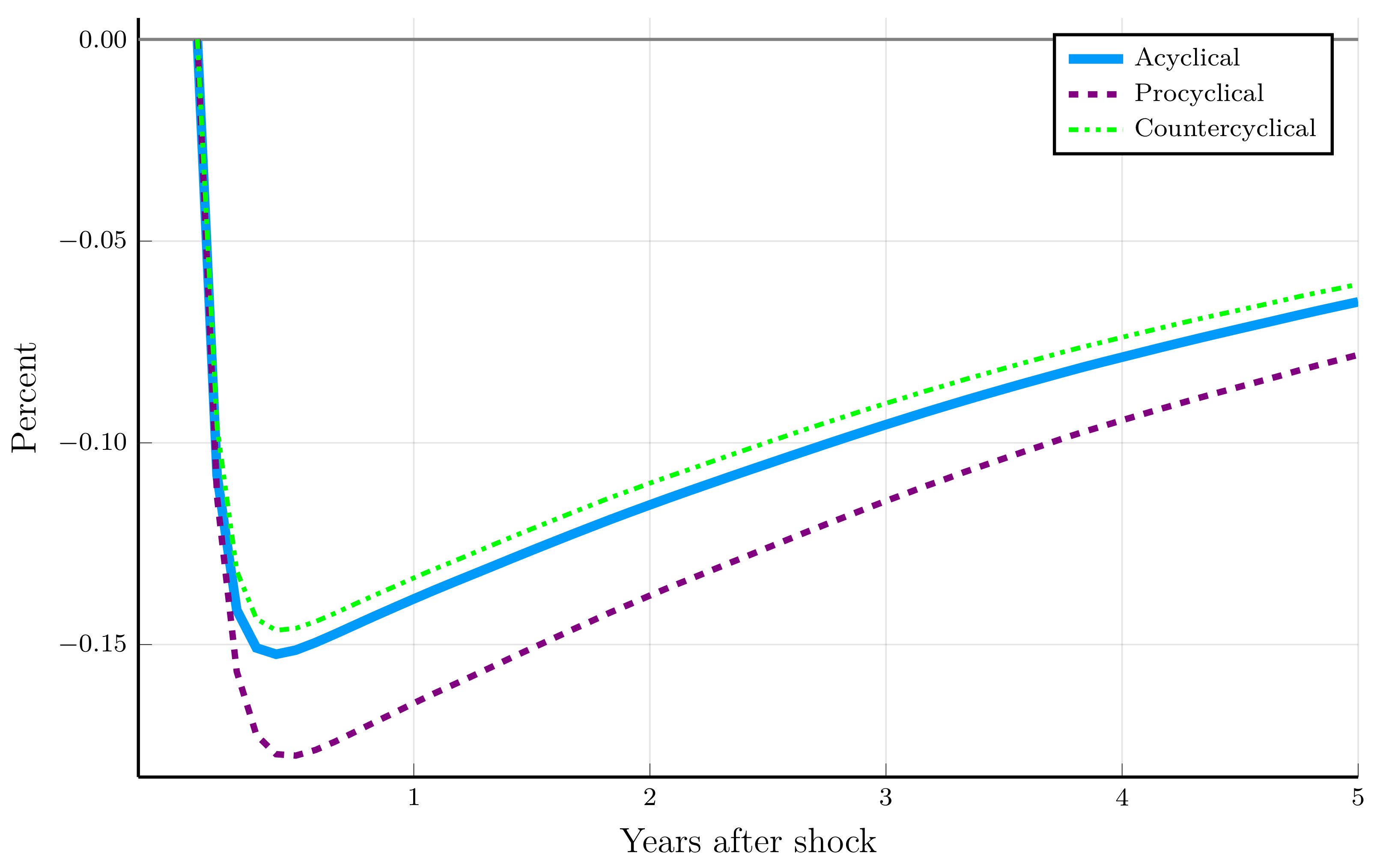
To further investigate how the economies indexed by creditors’ flow search costs respond to productivity fluctuations, I report impulse responses. Unlike linear dynamics, nonlinear dynamics depend on the state of the economy. I therefore compute the median unemployment rate from the ergodic distribution of each economy (reached by taking a sample of 10,000 years after an initial burn-in period of 100 years). From these starting values, I simulate the economy for 5 years over 5000 simulations for two different starting conditions. One uses standard normal draws to generate the initial shock in (24). The other replaces the initial value of the shock with a standard-normal draw plus 2 σ x . The average difference over the 5000 simulations is shown as the nonlinear impulse response. I conduct this exercise separately over the three economies.
The average impulse response of productivity is shown in Figure 3 (While the impulse responses differ across the three economies, the averages are nearly identical and visually indistinguishable). Figure 3 shows two important features. First, the shock is not large. Productivity on average jumps a little over 1 percent on impact. Second, the shock is persistent. After 5 years, productivity remains elevated.
Responses of unemployment to the productivity shocks are shown in Figure 4. On impact, in all three economies, in response to a positive productivity shock, unemployment falls rapidly. Around half a year after the shock, unemployment reaches its minimum. Unemployment in the acyclical economy falls around 15 basis points. For the next several years, unemployment is lower. The persistence of the productivity shock translates to the persistence of the response of unemployment.
The main result is the magnitudes of the responses across the three economies. The acyclical impulse response function falls between the countercyclical and procyclical impulse response functions; that is, the blue line falls between the dotted green line and the broken purple line. Countercyclical costs minify the response of unemployment to changes in productivity, while procyclical costs magnify the response of unemployment to changes in productivity. The effect is asymmetric. The difference between the cyclical economy and the procyclical economy is greater in absolute magnitude than the difference between the cyclical economy and the countercyclical economy; that is, the dotted green line is close to the solid blue line, whereas, the broken purple line is further from the solid blue line. Result 4 summarizes these results.
Result 4. 
Relative to acyclical hiring costs associated with the search for financing, for conventional parameter values, procyclical costs magnify the response of unemployment to productivity changes, and countercyclical costs minify the response of unemployment to productivity changes. Compared to countercyclical costs, procyclical costs have a larger effect.

4. Discussion

The relationship between financial markets and labor-market dynamics has been investigated by Ernst (2019). Using data on labor-market outcomes from 20 Organisation for Economic Co-operation and Development countries, Ernst (2019) finds that financial development predicts more labor-market turbulence. This evidence is consistent with the model here.
In addition, Ernst (2019) finds that the development of financial markets has a “significant albeit ambiguous influence on unemployment dynamics.” The decomposition of fluctuations in labor-market tightness summarized in Result 3 also points to understanding more about how costs of credit affect labor-market dynamics. In particular, it may be important to understand how credit markets interact with other features of the labor market. Chairassamee et al. (2023), for example, describe how state-level taxes within the United States affect unemployment. And Zhang and Lin (2025) use an larger-scale dynamic, stochastic, general-equilibrium model to understand how government financing affects the economy. In their model, the government expends resources to compete for employees. Understanding how taxes and government-sector employment affect labor-market dynamics and how these features interact with financing may help make progress on understanding the observed cyclical behavior of the United States labor market.
Links between credit-market cyclicality and job creation suggest a connection with macroprudential policy, which aims to ensure stability of the financial system. At the risk of oversimplifying slightly, the model provides a straightforward interpretation of the effect credit costs have on job creation. The cost of search in the credit market acts mechanically like a one-time hiring cost. This can be seen, for example, in the job-creation condition in (16). Competitive efforts by firms drive the expected cost of search (given on the left side) to become equal to the expected profits from a productive match with an employee (given on the right side). If the terms involving K were replaced by H, say, a one-time hiring cost independent of the state of the economy, then the model would be nearly identical to the models studied by Mortensen and Nagypál (2007) and Pissarides (2009).13 (The algebra would be even clearer if K were acyclical.) This suggests thinking about credit costs like one-time hiring costs.
This interpretation offers clear policy prescriptions. In times of economic distress, lowering the cost of credit is paramount for promoting job creation. The conclusion is consistent with evidence presented by Ernst (2019), who finds that transitions from unemployment to employment are positively related to credit growth. Additional evidence is provided by Chodorow-Reich (2014), who uses a novel dataset that links loans to employment. Poor financial health of lenders reliably and meaningfully predicts lower employment.14

5. Conclusions

The main message of this paper is that cyclical credit costs can magnify or minify how unemployment responds to changes in productivity. My conclusion is based on a straight-forward extension of the extremely important model set out by Wasmer and Weil (2004) and Petrosky-Nadeau and Wasmer (2013). My analysis attempted to connect compositional issues that naturally arise in financial markets over the business cycle to unemployment dynamics. I did this by allowing the cost of search incurred by creditors looking to finance production in the labor market to vary with the state of the aggregate economy.
The set of parameter values I investigated imply
  • procyclical credit costs magnify unemployment volatility, while
  • countercyclical credit costs minify unemployment volatility.
The model is nonlinear, and my calibration is not definitive. Nevertheless, the potential for cyclical credit costs to magnify responses of unemployment to changes in productivity and the large swings in unemployment that are observed in the data suggest exploring cyclical credit costs as a key feature of labor-market dynamics.
As Petrosky-Nadeau and Wasmer (2013) highlight, the key feature of the models I considered here is a component of hiring that is independent of labor-market tightness. This component arises from introducing a financial sector to a DMP search-and-matching model of the labor market. Search for credit acts like a fixed hiring cost and amplifies unemployment volatility. And, it offers a solution to the unemployment-volatility puzzle (Ljungqvist & Sargent, 2017; Pissarides, 2009). Improved macroeconomic modeling based on these insights means policymakers can better address unemployment, a source of misery for many people.
Yet, given the complex issues having to do with composition and asymmetric information inherent in finance (House, 2006; Stein, 2003), this component of hiring may well depend on the state of the aggregate economy. This is the deep issue I investigated. The modeling of creditors’ costs, which captured key features of finance like durable relationships with creditors (Chodorow-Reich, 2014) and illiquidity arising from trade frictions (Diamond, 1990), was for this specific purpose. Surely this is a limitation of the model, but the qualitative results suggest exciting new directions for research. The framework given here may provide a waypoint for understanding how the composition of financial markets affects labor-market dynamics.

Funding

This research received no external funding.

Institutional Review Board Statement

Not applicable.

Informed Consent Statement

Not applicable.

Data Availability Statement

No new data were created or analyzed in this study. Data sharing is not applicable to this article.

Conflicts of Interest

The author declares no conflicts of interest.

Appendix A. Deriving the Expected Cost of Search

This section derives the condition listed in (16).
I start from the expression for J v t in (13), which I repeat here for convenience:
J v t = γ + 1 s c β E t q θ t J π t + 1 + 1 q θ t J v t + 1 .
Setting J v t = K x t andusing the definition of β c 1 s c 1 + r 1 , the latter can be expressed as follows:
K x t = γ + q θ t β c E t J π t + 1 + 1 q θ t β c E t J v t + 1 K x t + γ = q θ t β c E t J π t + 1 + 1 q θ t β c E t K x t + 1 K x t + γ = q θ t β c E t J π t + 1 + 1 q θ t β c E t K x t + 1 K x t + γ q θ t = β c E t J π t + 1 + 1 q θ t q θ t β c E t K x t + 1 .
Or equivalently,
K x t + γ q θ t 1 q θ t q θ t β c E t K x t + 1 = β c E t J π t + 1 .
Under the assumption that firms perceive costs K to be martingale, so that E t K x t + 1 = K x t , the latter can be written as follows:
K x t + γ q θ t 1 q θ t q θ t β c K x t = β c E t J π t + 1 .
The left side can be developed as follows:
γ q θ t + K x t q θ t 1 q θ t q θ t β c K x t = γ q θ t + 1 β c 1 q θ t q θ t K x t = γ q θ t + 1 + q θ t q θ t β c 1 q θ t q θ t K x t = γ q θ t + q θ t + 1 q θ t 1 β c q θ t K x t = γ q θ t + 1 + 1 q θ t 1 β c q θ t K x t .
Using the definition of β c = 1 s c 1 + r 1 , the latter can be written as follows:
γ q θ t + 1 + 1 q θ t 1 β c q θ t K x t = γ q θ t + 1 + 1 1 s c 1 + r 1 1 q θ t q θ t K x t = γ q θ t + 1 + 1 + r 1 + s c 1 + r 1 q θ t q θ t K x t = γ q θ t + 1 + r + s c 1 + r 1 q θ t q θ t K x t .
In summary,
γ q θ t + 1 + r + s c 1 + r 1 q θ t q θ t K x t = β c E t J π t + 1 ,
which is Equation (16) in the main text.

Appendix B. Job Creation

Appendix B.1. Deriving the Dynamic Condition for Job Creation

This section derives the dynamic job-creation condition in terms of the exogenous stochastic process for productivity and wages.
Starting from (16), straightforward algebra found in (A1) implies
γ + ω t K x t q θ t = 1 s c β E t J π t + 1 ,
where
ω t 1 β c 1 q θ t .
By iterating forward the expression for J π t in (14), I can develop the job-creation condition as follows:
γ + ω t K x t q θ t = β c E t x t + 1 w t + 1 + β c 1 s E t + 1 J π t + 2 + β c s E t + 1 J v t + 2 = β c E t x t + 1 w t + 1 + β c E t + 1 J π t + 2 β c s E t + 1 J π t + 2 J v t + 2 .
To make the problem tractable, I want to eliminate the expression for E t + 1 J π t + 2 J v t + 2 .
To do this, I start from the expression for J v given in (13):
J v t = γ + β c E t q θ t J π t + 1 + 1 q θ t J v t + 1 = γ + β c E t q θ t J π t + 1 + 1 q θ t J v t + 1 + β c E t J π t + 1 β c E t J π t + 1 = γ β c 1 q θ t E t J π t + 1 J v t + 1 + β c E t J π t + 1 .
Using the fact that J v t = K x t , the latter can be written as
K x t + γ β c E t J π t + 1 = β c 1 q θ t E t J π t + 1 J v t + 1
or
E t J π t + 1 J v t + 1 = K x t + γ β c E t J π t + 1 β c 1 q θ t .
The expression in (A4) can be iterated forward and substituted into the right side of the developing expression in (A3), yielding
β c E t x t + 1 w t + 1 + β c E t + 1 J π t + 2 + β c s K x t + 1 + γ β c E t + 1 J π t + 2 β c 1 q θ t + 1 = β c E t x t + 1 w t + 1 + β c E t + 1 J π t + 2 + s K x t + 1 + γ β c E t + 1 J π t + 2 1 q θ t + 1 .
Combining the terms on the right involving J π t + 2 yields the following expression:
β c E t x t + 1 w t + 1 + β c 1 s 1 q θ t + 1 E t + 1 J π t + 2 + s K x t + 1 + γ 1 q θ t + 1 .
Next, I substitute out the expression for E t + 1 J π t + 2 in the latter using (A2). Doing this yields the following:
β c E t x t + 1 w t + 1 + β c 1 s 1 q θ t + 1 1 β c γ + ω t + 1 K x t + 1 q θ t + 1 + s K x t + 1 + γ 1 q θ t + 1 = β c E t x t + 1 w t + 1 + 1 s 1 q θ t + 1 γ + ω t + 1 K x t + 1 q θ t + 1 + s K x t + 1 + γ 1 q θ t + 1
In summary, I started from (A3) and simplified the right side so that
γ + ω t K x t q θ t = β c E t x t + 1 w t + 1 + 1 s 1 q θ t + 1 γ + ω t + 1 K x t + 1 q θ t + 1 + s K x t + 1 + γ 1 q θ t + 1 .
The expression in (A5) can be simplified to Equation (17) in the main text.
Indeed, the terms in square brackets involving K yield the following expression:
1 s 1 q θ t + 1 γ + ω t + 1 K x t + 1 q θ t + 1 + s K x t + 1 + γ 1 q θ t + 1 = 1 q θ t + 1 s 1 q θ t + 1 γ + ω t + 1 K x t + 1 q θ t + 1 + s q θ t + 1 K x t + 1 + γ q θ t + 1 1 q θ t + 1 = γ + ω t + 1 K x t + 1 1 q θ t + 1 s + s q θ t + 1 K x t + 1 + γ q θ t + 1 1 q θ t + 1 = 1 q θ t + 1 γ + ω t + 1 K x t + 1 s γ + ω t + 1 K x t + 1 + s q θ t + 1 K x t + 1 + γ q θ t + 1 1 q θ t + 1 .
Replacing ω t + 1 = 1 β c 1 q ( θ t + 1 in the second term in the numerator, factoring out 1 q θ t + 1 , and simplifying yields the following:
1 q θ t + 1 γ + ω t + 1 K x t + 1 s 1 q θ t + 1 γ + K x t + 1 β c K x t + 1 q θ t + 1 1 q θ t + 1 = γ + ω t + 1 K x t + 1 s γ + K x t + 1 β c K x t + 1 q θ t + 1
At this point, the developing expression is
γ + ω t K x t q θ t = β c E t x t + 1 w t + 1 + γ + ω t + 1 K x t + 1 s γ + K x t + 1 β c K x t + 1 q θ t + 1 .
Adding and subtracting 1 β c K x t + 1 and using the notation x c = x t + 1 1 β c K x t + 1 , the latter can be written as follows:
γ + ω t K x t q θ t = β c E t x t + 1 c w t + 1 + γ + ω t + 1 K x t + 1 s γ + K x t + 1 1 β c + 1 β c q θ t + 1 K x t + 1 q θ t + 1 .
Then, using ω t + 1 = 1 β c 1 q θ t + 1 , canceling terms, and factoring out 1 s from the terms in the numerator yields the following:
γ + ω t K x t q θ t = β c E t x t + 1 c w t + 1 + γ 1 s + K x t + 1 1 s β c K x t + 1 1 s + q θ t + 1 K x t + 1 q θ t + 1 .
Finally, using k x t + 1 = 1 β c K x t + 1 , using the expression for job creation in the text. This result is summarized below.
In summary, the algebra yields the dynamic job-creation condition
γ + ω t K x t q θ t = β c E t x t + 1 c w t + 1 + 1 s γ + k x t + 1 q θ t + 1 + K x t + 1 ,
where
x t c x t 1 β c K x t = x t k x t ,
a variable reflecting the credit and labor markets. This is Equation (17) in the main text.

Appendix B.2. The Steady-State Job-Creation Condition

The job-creation condition in (17) in steady state becomes
γ + ω K q θ = β c x c w + 1 s γ + K 1 β c q θ + K γ + 1 β c 1 q θ K β c q θ K q θ = β c x c w + 1 s γ k q θ ,
where the second equality uses γ k γ + K 1 β c γ + k . Developing the left side yields
γ + K β c K + β c q θ K β c q θ K q θ = β c x c w + 1 s γ k q θ γ + 1 β c K q θ = β c x c w + 1 s γ k q θ
or
γ k q θ = β c x c w + 1 s γ k q θ ,
which yields a steady-state condition that mechanically behaves similarly to the conventional model.

Appendix C. An Expression for the Wage Rate

This section develops an expression for the wage earned by a worker. To do this, it will be useful to define the surplus generated from a match in the labor market:
S t = W n t W u t + J π t J v t = W n t W u t + J π t K x t ,
where (A7) uses J v t = K x t from (15). The Nash sharing rule in the text can then be expressed as follows:
W n t W u t = α S t and J π t J v t = J π t K x t = 1 α S t .
An expression for the wage rate can be developed using two expressions for S t . One comes from the expressions for W n t , W u t , and J π t in (10), (9), and (14). These terms can be used to write surplus as follows:
S t = x t z K x t + β c 1 s E t S t + 1 β f θ t α E t S t + 1 + β c E t J v t + 1 .
A second expression for S t uses 1 α S t = J π t J v t . This expression can be developed, using the expression for J π t given in (14) and J v t = K x t in (13), as follows:
1 α S t = x t w t + β c 1 s 1 α E t S t + 1 + β c E t J v t + 1 K x t .
Expressions (A9) and (A10) imply
x t w t + β c 1 s 1 α E t S t + 1 + β c E t J v t + 1 K x t = 1 α x t z K x t + β c 1 s E t S t + 1 β f θ t α E t S t + 1 + β c E t J v t + 1 .
Solving for w t yields
w t = α x t + 1 α z α K x t + α β c E t J v t + 1 + 1 α β f θ t α E t S t + 1 .
To develop this expression, I will use the Nash sharing rule in (A8), expressed as follows:
E t S t + 1 = 1 1 α E t J π t + 1 J v t + 1 .
The expression in brackets on the right side can be equivalently expressed using the result in (A4). Doing this yields
E t S t + 1 = 1 1 α K x t + γ β c E t J π t + 1 β c 1 q θ t .
This expression and the outcome from Nash bargaining, J v t + 1 = J π t + 1 1 α S t + 1 , can be used in the developing expression for the wage to yield the following:
w t = α x t + 1 α z α K x t + α β c K x t + γ β c E t J π t + 1 β c 1 q θ t + E t J π t + 1 + β f θ t α K x t + γ β c E t J π t + 1 β c 1 q θ t .
Finally, collecting terms involving E t J π t + 1 and substituting out E t J π t + 1 using (A2) yields the following expression:
w t = α x t c + 1 α z + γ + k x t 1 s c α θ t = α x t c + 1 α z + γ k 1 s c α θ t .
This is Equation (19) in the main text.
This expression agrees with the expression for the wage in the model analyzed by Petrosky-Nadeau and Wasmer (2017, p. 162), even though the cost of credit depends on aggregate productivity. The dependence on productivity makes the algebra behind the expression in (A11) much more tedious than in the case analyzed by Petrosky-Nadeau and Wasmer (2017). Further details are available upon request.

Appendix D. Comparative Statics Demonstrate Properties of DMP Models and Robustness

The properties of the model can investigated by varying the parameter values to see their effects on unemployment. These properties can be understood within the larger class of DMP models. I focus on unemployment, even though a parameter change affects the entire ergodic distribution, because the DMP class of models generates unemployment as an equilibrium outcome and, as of now, has become the standard model of equilibrium unemployment (a point, for example, recently emphasized by Kehoe et al., 2023). The exercise demonstrates that the results are robust to alternative parameterizations.
To understand how parameters affect unemployment, I focus on ergodic distributions of economies indexed by different parameter values. Instead of recalibrating for each economy the flow value of maintaining a vacancy to match steady-state statistics (as was done in Section 3.2.2), I hold constant γ and vary parameters in isolation. This allows me to see how a parameter shifts an economy’s levels of experienced unemployment. For each economy indexed by a different set of parameter values, I reach the ergodic distribution by solving the model by implementing the algorithm described in Section 3.2.1, simulating the economy for 100 years to reach the ergodic distribution, and taking the next 250 years of data to plot.
The data are shown in Figure A1. The figure shows unemployment against productivity for each economy. The data shown using blue dots correspond to the baseline economy. The parameters in the baseline economy are the same as in the acyclical economy shown in Figure 1. Over the 250 × 12 months of data, the average unemployment rate in the economy was 5.6 percent.
Figure A1. Unemployment from simulating economies indexed by different parameter values starting from ergodic distributions.
Jrfm 18 00477 g0a1
Relative to the baseline, I perturb several parameters. The data shown in purple pentagons show the effect of a higher value of nonemployment, z. When z rises 5 percent relative to the baseline, for any level of productivity, unemployment is higher. A higher level of the flow value of nonwork raises a worker’s asset value of unemployment. Unemployment is lower. As such, a worker is in a better bargaining position and is able to negotiate a higher wage. Higher wages discourage firms from posting vacancies, and unemployment is higher. On average, unemployment in the economy indexed by a 5 percent higher value of z is 6.4 percent.
Other parameters generate similar comparative statics. A higher separation rate experienced by workers, unsurprisingly, causes unemployment to rise. This is shown in Figure A1 using green stars. The value s is 25 percent higher than in the baseline economy. Unemployment, on average, rises from 5.6 percent to 7.2 percent. A lower labor-market matching parameter, ν , also raises unemployment rates. A lower ν reduces job-finding and job-filling rates for any given level of labor-market tightness. Unsurprisingly, for any level of productivity, unemployment is higher. When ν is half the baseline value, the average rate of unemployment rises from 5.6 percent to 8.2 percent. When a worker captures more of the surplus generated from a match with a firm, represented by a higher α , unemployment will be higher. The expression for wages in (19) indicates that a higher α raises a worker’s flow compensation. This makes posting a vacancy less profitable, which translates to higher unemployment. Figure A1 shows this dynamic using gray stars. When α is 50 percent higher than in the baseline economy, unemployment on average rises from 5.6 percent to 8 percent. These patterns demonstrate that the model offers an appealing description of how the labor market functions.
In addition, the patterns uncovered in the comparative-statics exercise exhibit a common characteristic. Changing a parameter value that raises unemployment uniformly shifts the productivity–unemployment relationship upward. This evidence suggests that the mechanics of the model are robust to changing parameter values.
A related question is whether changes in parameter values affect results across different parameterizations of credit-market cyclicality. To avoid excessive computation, I focus on the flow value of nonwork, z.15
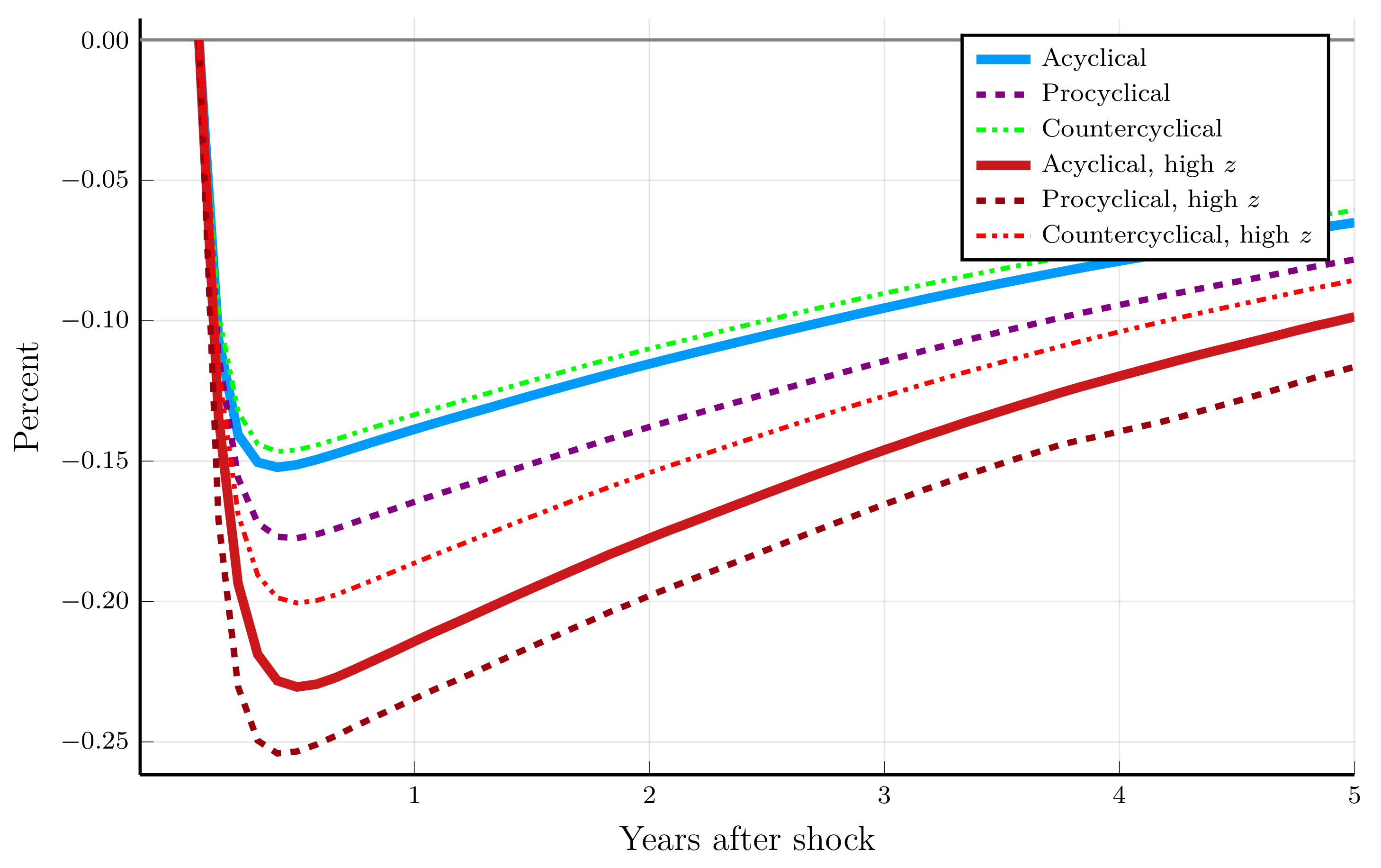
I investigate the consequences of increasing the value of nonwork by 5 percent. As shown in Figure A1, the average unemployment rate increases from 5.6 percent to 6.4 percent when the costs of credit are acyclical. Here, I investigate how increasing z interacts with credit-market cyclicality. For the cases where credit costs are procyclical and countercyclical, I solve the model using the algorithm listed in Section 3.2.1. Then, for each case, I compute the median unemployment rate from the ergodic distribution of each economy (reached by simulating the economy for 2000 years after throwing away the first 100 years of data). From these starting values, I simulate the economy for 5 years and repeat the simulation over 5000 replications. This is done for two different starting conditions. One uses standard normal draws to generate the initial shock in (24). The other replaces the initial value of the shock with a standard-normal draw plus 2 σ x . The average difference over the 5000 simulations is shown as the nonlinear impulse response. The nonlinear impulse responses are collected in Figure A2.
Figure A2. Nonlinear impulse responses of unemployment for two parameterizations of the flow value of nonwork.
Jrfm 18 00477 g0a2
Figure A2 shows how a higher value of nonemployment affects dynamics. The impulse responses are directly comparable to those from Figure 4, and I therefore repeat the analysis undergirding Figure 4 and report the results here (in these economies, z = 0.71 ). The three red lines show the effect of increasing z by 5 percent. For the baseline acyclical case, the solid red line shows the response of unemployment to a one-time, 2 σ x productivity shock for the economy characterized by acyclical credit costs. This line is comparable to the solid blue line. As predicted by theory, a higher z value implies that unemployment responds more to changes in productivity. This is the fundamental-surplus channel at work, and this channel applies to acyclical, procyclical, and countercyclical credit costs.
Compared to the acyclical economy, unemployment in the economy characterized by procyclical credit costs responds more to productivity changes than unemployment in the economy characterized by countercyclical credit costs. This can be see by comparing the broken dark-red line and the dotted bright-red line to the solid line. The pattern of cyclicality is consistent with Result 4—procyclical costs magnify the response of unemployment to productivity changes, and countercyclical costs minify the response of unemployment to productivity changes.
The main message of this exercise is that the qualitative conclusions are the same.

Notes

1
Daley et al. (2024) point out the pervasiveness of due diligence. They cite work by Lajoux and Elson (2011) and Cole et al. (2016) that documents the prevalence and costs of due diligence. Huang et al. (2023) document the labor costs of due diligence associated with mergers and acquisitions. If screening requires effort, then creditors’ flow cost of search can be thought of as costly effort, analogous to Shimer’s (2010) search-and-matching model in which a firm must devote some of its workforce to recruitment in order to hire an employee. Effort costs associated with screening are likely to be procyclical.
2
Ottonello and Song (2022) provide evidence consistent with the idea that financial intermediaries have greater access to funds in good states of the economy. They use high-frequency shocks to identify surprises in the market value of 18 financial intermediaries’ net worth. These financial shocks propagate to nonfinancial firms, but the propagation depends on the state of the aggregate economy, suggesting that financial intermediaries have access to more resources in good states.
3
Stein (2003) and Hall (2011) provide entry points to the the vast literature on financial markets. A recent example of how composition affects macroeconomic dynamics is provided by Guo et al. (2025). They document how a typical firm’s stock price falls by 1.2 percent on the day the firm announces its intent to sell equity and by 2.3 percent the following day. This evidence is interpreted as the effect of the firm’s revelation of private information. Private information creates a lemons-type problem, whereby firms need to signal their quality, making composition an important variable.
4
Although, Barnichon (2010) documents how the statistics presented by Shimer (2005) change when computed over later periods.
5
6
The vacancy rate is defined through the normalization of the labor force. If L t is the size of the labor force in period t, the number of matches per period is L t M t = M u t L t , v t L t . Because M exhibits constant returns to scale, canceling L t from both sides yields M t = M u t , v t , where v t is the vacancy rate in period t.
7
The repayment rule the creditor and entrepreneur agree upon solves
E t ψ t + 1 = arg max E v t E c t 1 α c B v t B c t α c .
Straightforward differentiation yields the result in (12). It is also straightforward to derive an expression for E t ψ t + 1 , but this is not needed for the analysis. The sharing rule in (12) is the essential component.
8
Further algebraic details can be found in Appendix B.1.
9
Further algebraic details can be found in Appendix C of the appendix.
10
Ryan (2023) shows how this condition can be interpreted as the value of posting an initial vacancy that is immediately filled.
11
The derivation uses that fact that 1 λ L 1 = 1 + λ L 1 + λ 2 L 2 + for some constant λ .
12
In Appendix D, I investigate increasing z, the flow value of nonwork.
13
14
Chodorow-Reich (2014) documents these relationships around the Great Recession (see also Duygan-Bump et al., 2015; Montoriol-Garriga & Wang, 2011). Chodorow-Reich et al. (2022) provide evidence about US lending around COVID-19. Adam (2024) provides evidence on access to finance in Saudi Arabia.
I thank an anonymous referee for making the connection to macroprudential policy.
15
The choice of this parameter value has generated much interest. In particular, Hagedorn and Manovskii (2008) calibrated a worker’s value of nonwork to be around 95 percent of the wage, consistent with the idea that a marginal worker is indifferent between work and nonwork in traditional, non-matching models of the labor market. Under this calibration, the model can generate the observed cyclicality of labor-market tightness. Yet, the notion that there is little improvement in a worker’s welfare from transitioning from unemployment to employment may be hard to accept. There are other criticisms (Pissarides, 2009). Shimer (2005), Costain and Reiter (2008), and Ljungqvist and Sargent (2017) provide more context.

References

  1. Adam, N. A. (2024). Perceived risk and external finance usage in small-and medium-sized enterprises: Unveiling the moderating influence of business age. Journal of Risk and Financial Management, 17(4), 150. [Google Scholar] [CrossRef]
  2. Barnichon, R. (2010). Productivity and unemployment over the business cycle. Journal of Monetary Economics, 57(8), 1013–1025. [Google Scholar] [CrossRef]
  3. Brügemann, B., & Moscarini, G. (2010). Rent rigidity, asymmetric information, and volatility bounds in labor markets. Review of Economic Dynamics, 13(3), 575–596. [Google Scholar] [CrossRef]
  4. Chairassamee, N., Hean, O., & Jabas, P. (2023). The financial impact of state tax regimes on local economies in the U.S. Journal of Risk and Financial Management, 16(10), 419. [Google Scholar] [CrossRef]
  5. Chodorow-Reich, G. (2014). The employment effects of credit market disruptions: Firm-level evidence from the 2008–2009 financial crisis. Quarterly Journal of Economics, 129, 1–59. [Google Scholar] [CrossRef]
  6. Chodorow-Reich, G., Darmouni, O., Luck, S., & Plosser, M. (2022). Bank liquidity provision across the firm size distribution. Journal of Financial Economics, 144(3), 908–932. [Google Scholar] [CrossRef]
  7. Christiano, L. J., Eichenbaum, M. S., & Trabandt, M. (2021). Why is unemployment so countercyclical? Review of Economic Dynamics, 41, 4–37. [Google Scholar] [CrossRef]
  8. Cole, R. A., Ferris, K. R., & Melnik, A. L. (2016). The direct cost of advice in M&A transactions in the financial sector. SSRN, 1458465. [Google Scholar] [CrossRef]
  9. Costain, J. S., & Reiter, M. (2008). Business cycles, unemployment insurance, and the calibration of matching models. Journal of Economic Dynamics and Control, 32(4), 1120–1155. [Google Scholar] [CrossRef]
  10. Daley, B., Geelen, T., & Green, B. (2024). Due diligence. The Journal of Finance, 79(3), 2115–2161. [Google Scholar] [CrossRef]
  11. Diamond, P. (1982). Wage determination and efficiency in search equilibrium. The Review of Economic Studies, 49(2), 217. [Google Scholar] [CrossRef]
  12. Diamond, P. (1990). Pairwise credit in search equilibrium. The Quarterly Journal of Economics, 105(2), 285–319. [Google Scholar] [CrossRef]
  13. Duygan-Bump, B., Levkov, A., & Montoriol-Garriga, J. (2015). Financing constraints and unemployment: Evidence from the Great Recession. Journal of Monetary Economics, 75, 89–105. [Google Scholar] [CrossRef]
  14. Ernst, E. (2019). Finance and jobs: How financial markets and prudential regulation shape unemployment dynamics. Journal of Risk and Financial Management, 12(1), 20. [Google Scholar] [CrossRef]
  15. Eyigungor, B. (2010). Specific capital and vintage effects on the dynamics of unemployment and vacancies. American Economic Review, 100(3), 1214–1237. [Google Scholar] [CrossRef]
  16. Garín, J., & Lester, R. (2019). The opportunity cost(s) of employment and search intensity. Macroeconomic Dynamics, 23(1), 216–239. [Google Scholar] [CrossRef]
  17. Gertler, M., & Trigari, A. (2009). Unemployment fluctuations with staggered nash wage bargaining. Journal of Political Economy, 117(1), 38–86. [Google Scholar] [CrossRef]
  18. Gomme, P., & Lkhagvasuren, D. (2015). Worker search effort as an amplification mechanism. Journal of Monetary Economics, 75, 106–122. [Google Scholar] [CrossRef]
  19. Guo, X., Ottonello, P., Winberry, T., & Whited, T. (2025). Firm heterogeneity and adverse selection in external finance: Micro evidence and macro implications. National Bureau of Economic Research. [Google Scholar] [CrossRef]
  20. Hagedorn, M., & Manovskii, I. (2008). The cyclical behavior of equilibrium unemployment and vacancies revisited. American Economic Review, 98(4), 1692–1706. [Google Scholar] [CrossRef]
  21. Hall, R. E. (2005). Employment fluctuations with equilibrium wage stickiness. American Economic Review, 95(1), 50–65. [Google Scholar] [CrossRef]
  22. Hall, R. E. (2011). The long slump. American Economic Review, 101(2), 431–469. [Google Scholar] [CrossRef]
  23. Hall, R. E. (2017). High discounts and high unemployment. American Economic Review, 107(2), 305–330. [Google Scholar] [CrossRef]
  24. Hall, R. E., & Milgrom, P. R. (2008). The limited influence of unemployment on the wage bargain. American Economic Review, 98(4), 1653–1674. [Google Scholar] [CrossRef]
  25. House, C. L. (2006). Adverse selection and the financial accelerator. Journal of Monetary Economics, 53(6), 1117–1134. [Google Scholar] [CrossRef]
  26. Huang, J., Yu, H., & Zhang, Z. (2023). External vs. in-house advising service: Evidence from the financial industry acquisitions. Journal of Risk and Financial Management, 16(2), 66. [Google Scholar] [CrossRef]
  27. Judd, K. L., Maliar, L., & Maliar, S. (2011). Numerically stable and accurate stochastic simulation approaches for solving dynamic economic models: Approaches for solving dynamic models. Quantitative Economics, 2(2), 173–210. [Google Scholar] [CrossRef]
  28. Kehoe, P. J., Lopez, P., Midrigan, V., & Pastorino, E. (2023). Asset prices and unemployment fluctuations: A resolution of the unemployment volatility puzzle. The Review of Economic Studies, 90(3), 1304–1357. [Google Scholar] [CrossRef]
  29. Kokonas, N. (2023). A note on the unemployment volatility puzzle. Oxford Economic Papers, 75(1), 55–74. [Google Scholar] [CrossRef]
  30. Lajoux, A. R., & Elson, C. M. (2011). The art of M&A (2nd ed.). McGraw-Hill. [Google Scholar]
  31. Ljungqvist, L., & Sargent, T. J. (2017). The fundamental surplus. American Economic Review, 107(9), 2630–2665. [Google Scholar] [CrossRef]
  32. Ljungqvist, L., & Sargent, T. J. (2018). Recursive macroeconomic theory (4th ed.). The MIT Press. [Google Scholar]
  33. Ljungqvist, L., & Sargent, T. J. (2021). The fundamental surplus strikes again. Review of Economic Dynamics, 41, 38–51. [Google Scholar] [CrossRef]
  34. Maliar, L., & Maliar, S. (2003). Parameterized expectations algorithm and the moving bounds. Journal of Business & Economic Statistics, 21(1), 88–92. [Google Scholar] [CrossRef]
  35. Montoriol-Garriga, J., & Wang, J. C. (2011). The great recession and bank lending to small businesses (Working Papers No. 11–16). Federal Reserve Bank of Boston. Available online: https://ideas.repec.org/p/fip/fedbwp/11-16.html (accessed on 20 August 2025).
  36. Mortensen, D. T. (1982). The matching process as a noncooperative bargaining (J. J. McCall, Ed.; pp. 233–258). University of Chicago Press. Available online: http://www.nber.org/books/mcca82-1 (accessed on 25 August 2025).
  37. Mortensen, D. T., & Nagypál, É. (2007). More on unemployment and vacancy fluctuations. Review of Economic Dynamics, 10(3), 327–347. [Google Scholar] [CrossRef]
  38. Ottonello, P., & Song, W. (2022). Financial intermediaries and the macroeconomy: Evidence from a high-frequency identification. National Bureau of Economic Research. [Google Scholar] [CrossRef]
  39. Petrosky-Nadeau, N. (2014). Credit, vacancies and unemployment fluctuations. Review of Economic Dynamics, 17(2), 191–205. [Google Scholar] [CrossRef]
  40. Petrosky-Nadeau, N., & Wasmer, E. (2013). The cyclical volatility of labor markets under frictional financial markets. American Economic Journal: Macroeconomics, 5(1), 193–221. [Google Scholar] [CrossRef][Green Version]
  41. Petrosky-Nadeau, N., & Wasmer, E. (2017). Labor, credit, and goods markets. The MIT Press. [Google Scholar]
  42. Petrosky-Nadeau, N., & Zhang, L. (2017). Solving the diamond-mortensen-pissarides model accurately. Quantitative Economics, 8(2), 611–650. [Google Scholar] [CrossRef]
  43. Pissarides, C. A. (1985). Short-run equilibrium dynamics of unemployment, vacancies, and real wages. The American Economic Review, 75(4), 676–690. [Google Scholar]
  44. Pissarides, C. A. (2000). Equilibrium unemployment theory (2nd ed.). MIT Press. [Google Scholar]
  45. Pissarides, C. A. (2009). The unemployment volatility puzzle: Is wage stickiness the answer. Econometrica, 77(5), 1339–1369. [Google Scholar] [CrossRef]
  46. Rogerson, R., & Shimer, R. (2011). Search in macroeconomic models of the labor market. In Handbook of labor economics (pp. 619–700). Elsevier. [Google Scholar] [CrossRef]
  47. Rogerson, R., Shimer, R., & Wright, R. (2005). Search-theoretic models of the labor market: A survey. Journal of Economic Literature, 43(4), 959–988. [Google Scholar] [CrossRef]
  48. Ryan, R. (2023). Responses of unemployment to productivity changes for a general matching technolog. Economics Bulletin, 43(4), 1749–1958. [Google Scholar]
  49. Ryan, R. (2024). Unemployment volatility: When workers pay costs upon accepting jobs. International Journal of Economic Theory, 20, 303–333. [Google Scholar] [CrossRef]
  50. Shimer, R. (2005). The cyclical behavior of equilibrium unemployment and vacancies. American Economic Review, 95(1), 25–49. [Google Scholar] [CrossRef]
  51. Shimer, R. (2010). Labor markets and business cycles. Princeton University Press. [Google Scholar]
  52. Silva, J. I., & Toledo, M. (2009). Labor turnover costs and the cyclical behavior of vacancies and unemployment. Macroeconomic Dynamics, 13(S1), 76–96. [Google Scholar] [CrossRef]
  53. Silva, J. I., & Toledo, M. (2013). The unemployment volatility puzzle: The role of matching costs revisited. Economic Inquiry, 51(1), 836–843. [Google Scholar] [CrossRef]
  54. Stein, J. C. (2003). Agency, Information and Corporate Investment. In Corporate finance (pp. 111–165). Elsevier. [Google Scholar] [CrossRef]
  55. Wang, B. (2023). The fundamental surplus revisited. Review of Economic Dynamics, 51, 1–15. [Google Scholar] [CrossRef]
  56. Wasmer, E., & Weil, P. (2004). The macroeconomics of labor and credit market imperfections. American Economic Review, 94(4), 944–963. [Google Scholar] [CrossRef]
  57. Zhang, S., & Lin, Z. (2025). The General Equilibrium Effects of Fiscal Policy with Government Debt Maturity. Journal of Risk and Financial Management, 18(7), 396. [Google Scholar] [CrossRef]
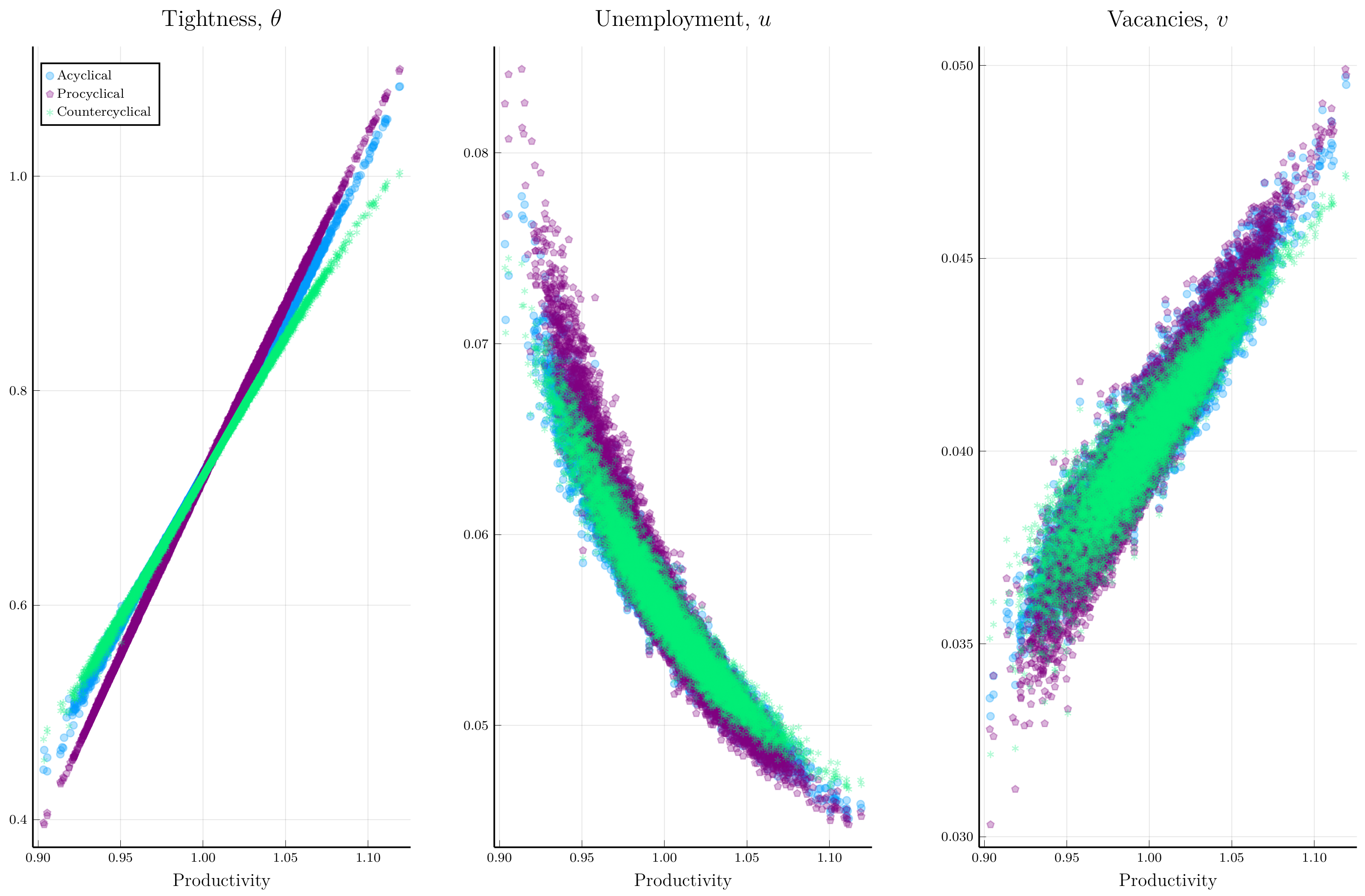
Figure 1. Tightness, unemployment, and vacancies from simulating the model starting from the ergodic distribution of acyclical, procyclical, and countercyclical parameterizations of the credit market.
Jrfm 18 00477 g001
Figure 2. Job-finding rates, job-filling rates, and wages from simulating the model starting from the ergodic distribution of acyclical, procyclical, and countercyclical parameterizations of the credit market.
Jrfm 18 00477 g002
Figure 3. Response of productivity to a 2-standard-deviation shock.
Jrfm 18 00477 g003
Figure 4. Nonlinear impulse responses of unemployment to a 2-standard-deviation shock to log productivity for acyclical, procyclical, and countercyclical parameterizations of the credit market.
Jrfm 18 00477 g004
Disclaimer/Publisher’s Note: The statements, opinions and data contained in all publications are solely those of the individual author(s) and contributor(s) and not of MDPI and/or the editor(s). MDPI and/or the editor(s) disclaim responsibility for any injury to people or property resulting from any ideas, methods, instructions or products referred to in the content.