Economic Attitudes and Financial Decisions Among Welfare Recipients: Considerations for Workforce Policy

Abstract

This study investigates economic decision-making behaviors among welfare recipients in Miami, Florida, by leveraging well-established experimental protocols: the Guessing Game, the Prudence Measurement Task, the Risk Aversion Task, and the Stag Hunt Game. For this purpose, our study defines financial decisions as the underlying individual preferences that serve as validated proxies for savings behavior, debt management, job-search intensity, and participation in cooperative finance. A central objective is to compare the behavior of welfare recipients to that of undergraduate students, a cohort typically used in experimental economics research. The analysis reveals significant differences between the two groups in strategic thinking and coordination, particularly across ethnic and gender lines. Non-Hispanic/Latino participants in Miami displayed significantly higher average guesses in the Guessing Game compared to their counterparts in Tucson, indicating potential discrepancies in the depth of strategic reasoning. Additionally, female participants in Tucson exhibited higher levels of coordination in the Stag Hunt Game compared to females in Miami, suggesting variance in cooperative behavior between these groups. Despite these findings, regression models demonstrate that location, gender, and ethnicity collectively account for only a small fraction of the observed variance, as evidenced by low R² values and substantial mean squared errors across all games. These results suggest that individual heterogeneity, rather than broad demographic variables, may be more influential in shaping economic decisions. This study underscores the complexity of generalizing findings from traditional student samples to more diverse populations, highlighting the need for further investigation into the socioeconomic factors that drive financial decision-making.

1. Introduction

Experimental economics has long relied on undergraduate students as the primary subject pool, raising a central methodological question: to what extent can findings derived from this homogenous group be generalized to broader societal populations? The external validity of student-based experiments has been rigorously scrutinized, with many studies indicating that when decontextualized tasks, typically used in laboratory settings, are applied to non-student populations, the results tend to mirror those from controlled environments. Artefactual field experiments (Harrison & List, 2004) and extra-laboratory experiments (Charness & Gneezy, 2012) have demonstrated this consistency (C. Camerer, 2011), although exceptions do exist (Belot et al., 2015; Cappelen et al., 2015). Notably, Fréchette and Schotter (2015) find that while there are discernible differences between students and professionals with domain-specific expertise, the behavioral patterns of the two groups are largely aligned, particularly when navigating standard economic tasks.

In this study, we extend this line of inquiry by replicating a series of well-established experimental protocols among welfare recipients enrolled in a welfare-to-work program in Miami, Florida. This population represents a demographic that is seldom engaged in experimental economic research, thus offering a robust test of the generalizability of findings typically observed in student populations. The welfare recipients we study are starkly distinct from the standard student sample in terms of socioeconomic status, life experiences, and exposure to economic decision-making frameworks. While previous field experiments (e.g., Cappelen et al., 2015) have explored non-student populations, few, if any, have systematically examined individuals from this socioeconomic stratum, making this study a stringent test of robustness. To facilitate a meaningful comparison, we juxtapose the behavioral responses of the Miami welfare recipients with a control group of undergraduate students from the University of Arizona, who participated in the same experimental tasks. The considerable disparity in socioeconomic background and life experiences between these two groups provides fertile ground for investigating whether decision-making principles—such as risk aversion, prudence, and beliefs about rationality—differ systematically. Additionally, we examine whether gender-based behavioral differences observed among students can be generalized to welfare recipients, and we further explore how Hispanic and non-Hispanic participants’ decisions compare within the welfare recipient group.

Our experimental design includes four well-known economic tasks: (a) the risk aversion measurement protocol of Holt and Laury (2002), (b) the prudence measurement task introduced by Noussair et al. (2014), (c) the Guessing Game or Beauty Contest (Nagel, 1995), and (d) a Stag Hunt coordination game. These paradigms are fundamental within the social sciences for probing various dimensions of economic behavior, including strategic thinking, risk preferences, and coordination. The choice to focus on welfare recipients is driven by their unique relevance to policy discussions around workforce development and financial independence. Understanding the economic attitudes, preferences, and decision-making processes of individuals reliant on public assistance is crucial for formulating interventions that can facilitate their transition into employment. More broadly, identifying the behavioral correlates of welfare dependency may aid in predicting which individuals are most at risk of prolonged welfare reliance, as well as those who are likely to transition successfully into the workforce. We employ correlational analysis to assess the data collected from these experiments. However, we acknowledge the inherent limitations of such an approach, particularly with respect to causality. It remains unclear whether any behavioral differences identified between welfare recipients and the student control group are a consequence of adverse life experiences or if they reflect pre-existing preferences and traits that preceded welfare dependency. Additionally, selection bias is a potential concern, as participation was voluntary, and we could not mandate involvement. That said, selection effects are common in both laboratory and field experiments, and we find no compelling reason to believe that this issue unduly influenced our results in this context.

1.1. The Tasks

Experimental methods in economics, originating in the mid-20th century, have advanced significantly in recent decades, transitioning from theory testing to a broad application in measuring individual preferences and comparing behaviors across population groups. In this study, we employ four experimental paradigms: the Guessing Game (Nagel, 1995), the Prudence Measurement Task (Noussair et al., 2014), the Risk Aversion Task (Holt & Laury, 2002), and the Stag Hunt Game, a coordination game rooted in game theory. These paradigms are not only foundational in experimental economics but also critical for understanding key economic behaviors, such as strategic thinking, prudence, risk aversion, and coordination behaviors central to workforce development and financial sustainability.

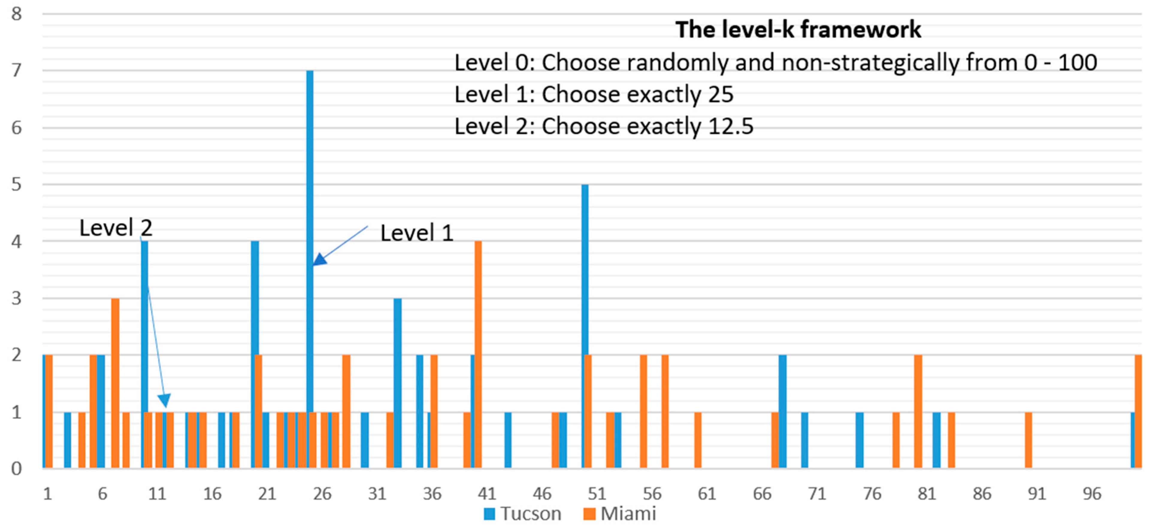
1.2. The Guessing Game: Measuring Strategic Thinking and Perceived Rationality

The Guessing Game, also known as the Beauty Contest, is designed to uncover insights into participants’ strategic thinking and their perceptions of others’ rationality. Nagel (1995) demonstrated that this game reveals individuals’ “depth of reasoning,” which reflects how many iterations of reasoning they apply to predict others’ behavior. The game involves guessing a number between 0 and 100, with the winner being the person whose guess is closest to a specified fraction (p) of the average guess. From a theoretical perspective, rational players would progressively eliminate dominated strategies, ultimately converging on zero as the Nash equilibrium. Iterated elimination of dominated strategies would lead to all players choosing zero, as rational actors recognize that no guess above zero would ever be optimal (Nagel, 1995). However, empirical evidence often diverges from this game-theoretic prediction, indicating limitations in the cognitive resources that individuals apply to such tasks (C. F. Camerer & Ho, 2015). This divergence may be explained by individuals relying on heuristic models when making decisions under strategic uncertainty. As suggested by Bozeman (2022), heuristic rules can often govern behavior, leading to rule compliance or deviations from strict rationality, especially when cognitive resources or time are limited. Bilancini et al. (2019) further explore the discrepancy between strategic behavior models and actual player behavior, suggesting that behavioral game theory better accounts for the systematic deviations observed in experimental settings. Additionally, Baron et al. (2020) highlight the importance of psychological testing in assessing and improving cognitive competencies, which is crucial for understanding the variance in strategic reasoning displayed by individuals in economic decision-making tasks such as the Guessing Game. In prior research, significant differences in strategic reasoning have been found between students and non-students. Belot et al. (2015) discovered that students exhibit a greater depth of reasoning than demographically representative non-student samples, supporting the hypothesis that welfare recipients, who differ from students in educational background and life experience, might display less strategic behavior in this task.

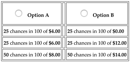
1.3. Prudence Measurement Task: Assessing Caution in Decision-Making

Prudence, a higher-order risk preference, is defined within the expected utility framework as a convex marginal utility function (Kimball, 1990). Research into the consistency of higher-order risk preferences has shown that individuals often exhibit consistent behavior regarding prudence, risk aversion, and temperance, supporting the theoretical models applied in experimental economics (Deck & Schlesinger, 2014). It reflects the propensity of individuals to exhibit greater caution when exposed to risk in lower-wealth states. Eeckhoudt and Schlesinger (2006) describe prudence in terms of risk apportionment—where prudent individuals prefer to face risks in high-wealth states rather than in low-wealth states. This notion of prudence has been further supported by experimental findings, which show that individuals often display higher levels of prudence when faced with gains and losses, as demonstrated by Brunette and Jacob (2019), who explored the relationship between prudence, risk aversion, and temperance in different economic contexts.

In the Prudence Measurement Task, participants choose between lotteries designed to test their preference for deferring risk to higher wealth states. The choices reflect whether individuals prioritize prudence when making financial decisions. In this study, we utilized two lotteries with different payoffs in Miami and Tucson, adjusting the monetary values to half for the Tucson cohort. Empirical studies suggest that prudence correlates with socioeconomic status. Noussair et al. (2014) found that prudent decision-making is positively associated with higher educational attainment, wealth accumulation, and financial stability. This suggests that university students, who generally have higher education levels than welfare recipients, might exhibit greater prudence. Natasha and Soenarno (2018) confirm that highly prudent individuals are more cautious in risk-taking, supporting the notion that prudence significantly impacts financial decision-making and may differentiate the welfare recipients from the student sample.

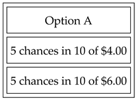
1.4. Risk Aversion Measurement Task: Evaluating Risk Preferences

Holt and Laury (2002) developed a widely used protocol to measure risk aversion through a series of binary choices between two lotteries. Participants choose between a relatively safe lottery and a riskier alternative, with the probability of the higher payoff increasing across ten choices. This design allows for the identification of risk-neutral, risk-averse, or risk-seeking behavior based on the number of safe choices made. The literature on the relationship between socioeconomic status and risk aversion is mixed. Breen et al. (2014) found that risk-averse individuals are less likely to pursue higher education, while Deckers et al. (2015) report that individuals from higher socioeconomic backgrounds tend to be less risk-averse. Gender and ethnicity are also known to influence risk preferences, with women and certain ethnic groups exhibiting higher risk aversion on average (Eckel & Grossman, 2008; Holt & Laury, 2002). In this study, we hypothesize that there will be no significant differences in risk aversion between the welfare recipients in Miami and the university students in Tucson. Recent findings by André et al. (2022) highlight that both risk aversion and ambiguity aversion can significantly shape financial decisions, particularly in the context of saving and annuity choices, further reinforcing the need to examine these preferences across varying demographic backgrounds and their impact on long-term financial behavior.

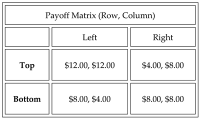
1.5. The Stag Hunt Game: Coordination and Strategic Uncertainty

The Stag Hunt Game, rooted in the philosophical writings of Jean-Jacques Rousseau and formalized by Skyrms (2004), is a two-player coordination game that examines the tension between individual risk and mutual cooperation. In the game, two hunters can either collaborate to catch a stag, which yields a higher payoff but requires mutual cooperation or individually hunt a rabbit, a lower payoff but risk-free option. The game features two Nash equilibria: a Pareto-optimal equilibrium (both players hunt the stag) and a risk-dominant equilibrium (both players hunt rabbits). Coordination on the Pareto-optimal outcome depends on each player’s belief that the other will also cooperate. However, if there is uncertainty about the other player’s strategy, individuals may opt for the risk-dominant equilibrium, leading to suboptimal outcomes.

Existing literature highlights the complexities of coordination under strategic uncertainty. Dipartimento and Marchetti (2019) found that players tend to choose the risk-dominant strategy when faced with ambiguity about the other player’s intentions. The Stag Hunt game thus serves as an ideal tool for measuring coordination and strategic uncertainty within different demographic groups. Avramopoulos (2018) suggests that incremental deployability can play a role in how individuals adapt to coordination challenges over time, which is relevant in the context of the Stag Hunt Game, where participants must continuously adjust their strategies based on perceived cooperation from others. We hypothesize that welfare recipients and students will exhibit similar levels of coordination, given the simplicity of the game structure.

2. Experimental Procedures

In Miami, four experimental sessions were conducted in July 2015, yielding a total of 56 participants. The initial session comprised eight participants, while the subsequent three sessions had 16 participants each. The sessions were hosted at Youth Co-op CareerSource South Florida—one of the primary administrators of the Temporary Assistance for Needy Families (TANF) program in Miami-Dade County, Florida. Recruitment of participants was facilitated through collaboration with case managers at the workforce center, allowing researchers to introduce the study during the center’s standard orientation sessions for welfare recipients. A 20-min briefing provided potential participants with an overview of the study, compensation, research limitations, and details on the consent process. This approach aligns with best practices in experimental economics, which emphasize transparency and informed consent (Charness et al., 2013).

Given the diversity of the Miami population, the sessions were conducted in both English and Spanish to accommodate linguistic preferences. All participants voluntarily agreed to participate, signing consent forms in their preferred language. The demographic composition of the Miami sample was predominantly female (61%) and Hispanic (62%). For English-speaking participants, the experiment was fully computerized using the Veconlab platform, developed by the University of Virginia (Holt, 1999), ensuring consistent and reliable data collection. For Spanish-speaking participants, the experiment was administered using pen and paper, with responses later entered into the system by bilingual experimenters to ensure accurate data recording. Bilingualism in the experimental process was vital to maintaining linguistic fidelity and ensuring that instructions and responses were accurately translated and understood by participants.

The second sample consisted of 58 undergraduate students from the University of Arizona. These sessions were conducted at the Economic Science Laboratory in February 2016. The recruitment of participants was carried out using the lab’s established participant pool, with voluntary participation encouraged through standard methods (Falk & Heckman, 2009). In this sample, 53% of participants were female, and 22% identified as Hispanic. The sessions were conducted entirely in English and, like the Miami sessions, utilized the Veconlab platform for data collection. The instructions used to implement these economic experiments were developed based on established methodologies from the experimental economics literature (C. F. Camerer & Ho, 2015; Fréchette & Schotter, 2015). They also incorporate technical language sourced from the VeconLab website (Holt, 2005). For the full English version of the instructions, see Appendix A.

Additional demographic characteristics further highlight the distinctiveness of the two study populations. In terms of age, welfare recipients from Miami had a mean age of 37.2 years (SD = 8.5), whereas the undergraduate student participants from Tucson had a mean age of 20.3 years (SD = 1.8), reflecting a substantial generational gap. Educational attainment also varied markedly: among welfare recipients, 20% had not completed high school, 50% held a high school diploma or GED, and 30% had pursued some college or vocational training. In contrast, all Tucson participants were actively enrolled in university programs, with declared majors in Economics (45%), Business (25%), and Psychology or other Social Sciences (30%). Finally, participants’ life contexts differed significantly. The Miami cohort was engaged in the TANF workforce-readiness program for an average of six months (SD = 3.1), indicating active involvement in government-supported employment preparation. Meanwhile, the Tucson students were recruited from the university’s standard laboratory participant pool, with no reported participation in welfare programs. These demographic contrasts underscore the divergent lived experiences of the two groups, reinforcing the significance of the behavioral convergence observed in the study.

In this paper, the term financial decisions specifically denotes the behavioral preferences and decision-making processes elicited through our four incentivized experimental tasks. Although these tasks do not directly measure actual financial transactions, prior literature has robustly validated their role as proxies for critical real-world financial behaviors. Thus, we utilize these tasks as empirically grounded indicators of financial decision-making relevant to welfare-to-work and workforce-development contexts.

To minimize potential selection bias, recruitment in Miami was conducted directly in partnership with TANF case managers during mandatory orientation and training sessions, ensuring that all eligible welfare recipients present had the opportunity to participate. This approach reduces reliance on passive or opt-in recruitment strategies and helps capture the diversity of the active welfare-to-work population. We also compared the demographic characteristics of our study sample to the broader eligible population and found no significant differences in age, gender, or ethnicity, supporting sample representativeness. While some degree of selection bias is unavoidable in any voluntary study, our recruitment design, coupled with guaranteed participation payments and bilingual accessibility, aligns with best practices in experimental and field economics for external validity (Harrison & List, 2004; Charness et al., 2013).

2.1. Session Structure and Compensation

The experimental sessions in Miami lasted approximately three hours, whereas sessions in Arizona were slightly shorter, averaging 2.5 h. Participants were financially compensated based on their performance, with Miami participants earning between USD 30.00 and USD 70.00, and Arizona participants earning between USD 20.00 and USD 50.00. These payment schemes adhered to the guidelines for incentivizing participants in experimental economics, where compensations are designed to balance motivation without causing undue financial hardship (C. F. Camerer & Hogarth, 1999). The design ensured that no participant could lose money in any of the tasks, thereby maintaining participant engagement while reducing the potential for adverse emotional responses that might skew the results.

The sequence of tasks was consistent across both locations. Participants first engaged in the Guessing Game, followed by the Prudence Measurement Task, the Risk Aversion Task, and, finally, the Stag Hunt game. This structured sequence was designed to minimize order effects, a common concern in experimental economics where earlier tasks can potentially influence behavior in subsequent tasks (Keren & Raaijmakers, 1988). Although randomization of task order is often suggested to mitigate these effects (Gneezy & Rustichini, 2000), it was determined that the order effects in this experiment would be negligible due to the relatively short duration of the tasks and the breaks between games. Furthermore, the consistent implementation of the games across both student and welfare recipient groups, coupled with the introduction of practice rounds, ensured that any practice or fatigue effects were likely uniform across all participants.

2.2. Data Collection and Coding

Data were coded systematically to facilitate subsequent analysis. Gender was coded as Male = 1 and Female = 0, Ethnicity as Hispanic = 1 and Non-Hispanic = 0, and Location as Miami = 1 and Tucson = 0. These coding conventions are standard in experimental economics and behavioral finance research, where categorical variables such as gender, ethnicity, and location are frequently used to examine group-level differences in economic behavior (Greene, 2012).

The data were subsequently analyzed using SPSS version 27.0, a robust statistical software package frequently employed in behavioral and experimental economics research (Field, 2024). This software was used to conduct both descriptive and inferential analyses, ensuring that the findings were statistically rigorous and suitable for publication in high-ranking economic journals.

2.3. Consideration of Order Effects

The potential influence of order effects was thoroughly considered in the experimental design. Order effects occur when earlier treatments or tasks affect participants’ responses in later tasks, a common concern in experimental and social science research (Campbell & Stanley, 2015). Researchers debated whether randomizing the order of the games would alleviate this issue, but concluded that the effects would be minimal due to the structured breaks, practice sessions, and relatively short duration of each game. The consistency in experimental conditions across sessions and locations ensured that any potential order effects would be uniformly distributed across the participant pool (List, 2007). Moreover, both groups—students and welfare recipients—were novices to the experimental tasks, meaning that any potential learning or fatigue effects would be comparable across groups. Given the brief and straightforward nature of the tasks, as well as the absence of complex inter-task dependencies, the decision to retain a fixed task sequence was deemed appropriate. This approach is supported by previous studies in experimental economics, which suggest that the potential for order effects diminishes in relatively short, self-contained games (Croson, 2005).

3. Results

This section provides an analysis of

Table 1. Descriptive Statistics of The Decisions Across the Four Games.

		Guessing Game (Average Guess/StD)	Prudence Measurement Task (Avg. % Prudent Choices)	Risk Aversion Measurement Task (Avg. # Safe Choices/StD)	Stag Hunt Game (% Playing Pareto Optimal Action/StD)
Range of responses		[0, 100]	[0, 1]	[0, 10]	[0, 1]
Miami	All Miami	36.30 (25.58)	55%	5.48 (2.10)	0.71 (0.46)
	Male	35.64 (25.73)	55%	5.36 (1.92)	0.77 (0.43)
	Female	36.74 (25.86)	56%	5.56 (2.23)	0.68 (0.48)
	Hispanic/Latino	29.83 (22.20)	60%	5.57 (2.48)	0.74 (0.44)
	Non-Hispanic/Latino	47.10 (27.67)	48%	5.33 (1.28)	0.67 (0.48)
Tucson	All Tucson	31.98 (21.42)	52%	5.55 (1.47)	0.84 (0.37)
	Male	28.04 (17.54)	44%	6.00 (1.47)	0.78 (0.42)
	Female	35.42 (24.06)	58%	5.16 (1.37)	0.90 (0.30)
	Hispanic/Latino	29.08 (20.63)	54%	5.85 (1.14)	0.92 (0.28)
	Non-Hispanic/Latino	32.82 (21.80)	51%	5.47 (1.55)	0.82 (0.39)

Note: Standard Deviation (StD).

and

Table 2. Estimates of Behavioral-Task Scores.

	Guessing Game	Prudence Task	Risk-Aversion Task	Stag-Hunt Game
Location (Miami = 1)	8.561 †	−0.010	−0.164	−0.997 †
	(4.744)	(0.414)	(0.371)	(0.517)
Gender (Female = 1)	−4.281	−0.315	0.340	−0.120
	(4.379)	(0.382)	(0.343)	(0.466)
Ethnicity (Minority = 1)	−11.355	0.335	0.297	0.517
	** (4.791)	(0.420)	(0.375)	(0.513)
Constant	36.521	0.141	5.327	1.651
	*** (3.803)	(0.414)	*** (0.298)	*** (0.436)
R2	0.065	0.014	0.015	0.034
Observations	114	114	114	114

Notes: Significance is flagged with the conventional asterisks: † p < 0.10, ** p < 0.01, *** p < 0.001. and standard errors clustered by experimental sessions in parentheses. The Guessing-Game score (0–100) and the count of safe lottery choices (0–10) are analyzed with OLS, whereas the binary outcomes from the Prudence Task and Stag-Hunt Game are estimated with Probit, reported as average marginal effects.

, which summarize the behavioral outcomes across four experimental games (the Guessing Game, Prudence Measurement Task, Risk Aversion Measurement Task, and Stag Hunt Game) for participants from two locations: Miami and Tucson. The data are further disaggregated by gender and ethnicity. Additionally, regression analyses are conducted to assess the impact of location, gender, and ethnicity on the performance in these games.

3.1. The Guessing Game—Strategic Thinking and Perceived Rationality of Others (Average Guess)

Table 1 shows that Miami participants had a higher average guess (36.30) compared to Tucson participants (31.98), suggesting that Tucson participants demonstrated slightly more strategic thinking. A lower guess implies greater depth of reasoning, as participants attempt to predict the guesses of others. The standard deviations (Miami: 25.58; Tucson: 21.42) indicate high variability in both groups, signaling diverse levels of sophistication within each group (Evgenia & Neycheva, 2014). Males in both locations exhibited slightly lower average guesses (Miami: 35.64; Tucson: 28.04) than females, suggesting that males tended to exhibit more strategic reasoning. The difference is particularly notable in Tucson, where males had an average guess significantly lower than females (35.42 for Tucson females), indicating a larger gender gap in strategic thinking. Non-Hispanic/Latino participants in Miami had a substantially higher average guess (47.10) compared to their counterparts in Tucson (32.82), implying lower levels of strategic thinking among non-Hispanic/Latinos in Miami. Conversely, Hispanic/Latino participants in both locations exhibited similar levels of strategic thinking, with averages close to 30.

Table 2 illustrates that the location variable is significant at the 10% level (B = 8.561, Std Error = 4.744), suggesting that being in Miami leads to a higher guess, indicative of less strategic reasoning. Ethnicity also has a significant negative effect on guesses (B = −11.355, Std Error = 4.791, p < 0.05), indicating that Hispanic/Latino participants tend to make lower (more strategic) guesses than non-Hispanic/Latino participants. The gender effect, while present, is not statistically significant.

Table 3. Comparison of Guessing Game (Average Guess).

Variables	Mean Value		Mean Difference	t-Value	p-Value
	Miami	Tucson
All	36.30	31.98	4.32	0.979	0.330
Male	35.64	28.04	7.60	1.226	0.226
Female	36.74	35.42	1.32	0.212	0.833
Hispanic/Latino	29.83	29.08	0.75	0.106	0.916
Non-Hispanic/Latino	47.10	32.82	14.27	2.270	0.027 *

Note: * significant at 10%.

supports the findings from Table 1 and Table 2 by reinforcing the importance of ethnicity in determining strategic thinking, particularly for non-Hispanic/Latino participants. It also confirms that while Tucson participants generally exhibit more strategic reasoning, the differences are not always statistically significant. Gender differences remain negligible across the analyses. The significant gap between non-Hispanic/Latino participants in Miami and Tucson suggests that future research could benefit from exploring additional demographic factors, such as education and socioeconomic status, to better understand these behavioral differences.

Figure 1 likely reveals that Tucson participants exhibited a more strategic, concentrated guessing pattern, while Miami participants showed more variability in their choices, with less emphasis on lower guesses. The distribution patterns in Figure 1 align with the findings from Table 1, Table 2 and Table 3, particularly highlighting the more strategic thinking observed in Tucson, especially among the non-Hispanic/Latino participants, compared to Miami.

3.2. Prudence Measurement Task—(Avg % Prudent Choices)

As shown in Table 1, participants from Miami exhibited slightly higher prudence (55%) compared to Tucson (52%). This small difference indicates a marginally greater preference for caution in financial decisions among Miami participants. Females were generally more prudent than males, especially in Tucson, where the gender gap was more pronounced (58% for females vs. 44% for males). This finding aligns with established literature, which suggests that women tend to be more risk-averse and prudent in financial decision-making (Eckel & Grossman, 2008) (Ebert & Wiesen, 2011). In Miami, Hispanic/Latino participants displayed more prudence (60%) than non-Hispanic/Latino participants (48%). A similar pattern is observed in Tucson, where Hispanic/Latino participants exhibited slightly higher prudence (54%) compared to non-Hispanic/Latino participants (51%).

Table 2 shows that none of the variables (location, gender, or ethnicity) significantly impact the prudence score, as reflected by the low R² value (0.014), suggesting that these demographic factors do not explain much of the variation in prudent behavior. This indicates that prudence might be influenced by other, unobserved factors.

Table 4. Comparison of Prudence Choice (Average % of Prudent Choices).

Variables	Mean Value		Mean Difference	t-Value	p-Value
	Miami	Tucson
All	0.55	0.52	0.04	0.386	0.701
Male	0.55	0.44	0.10	0.693	0.492
Female	0.56	0.58	−0.02	−0.175	0.862
Hispanic/Latino	0.60	0.54	0.06	0.377	0.708
Non-Hispanic/Latino	0.48	0.51	−0.03	−0.260	0.795

provides a comparison of the average percentage of prudent choices between participants in Miami and Tucson, broken down by gender and ethnicity. Table 4 supports the findings generated in Table 1 and Table 2, showing no significant differences in prudence based on location, gender, or ethnicity. While there are small, non-significant variations in the average percentage of prudent choices, these differences are consistent with the earlier results. The relatively stable prudence levels across all demographic groups suggest that prudence is less affected by these variables in this experimental setting.

The lack of significant differences across all categories suggests that prudence is relatively stable in the sample. The minimal variation in prudence choices between groups indicates that demographic factors such as gender, location, or ethnicity do not strongly influence prudent decision-making in this experimental setup. This finding aligns with the low R² value in Table 2’s regression model, suggesting that prudence may be influenced by other unmeasured factors such as individual experience, education, or cognitive ability.

3.3. Risk Aversion—Number of Safe Choices

Table 1 shows that both locations showed similar levels of risk aversion, with Miami participants making an average of 5.48 safe choices and Tucson participants making 5.55 safe choices. This suggests that location does not have a substantial effect on risk preferences. Tucson males displayed a higher average number of safe choices (6.00) compared to Miami males (5.36), indicating slightly more risk aversion. Meanwhile, Miami females were more risk-averse than Tucson females, making 5.56 safe choices on average compared to 5.16 in Tucson. Hispanic/Latino participants in both locations were more risk-averse than their non-Hispanic/Latino counterparts. In Miami, Hispanic/Latino participants made 5.57 safe choices compared to 5.33 for non-Hispanic/Latinos. Similarly, in Tucson, Hispanic/Latinos made 5.85 safe choices compared to 5.47 for non-Hispanic/Latino participants. These findings align with prior studies on risk preferences, such as Haering et al. (2020), which explored the consistency of higher-order risk preferences, indicating that prudence and risk aversion behaviors are largely stable across different contexts.

Table 2 illustrates that, similar to the Prudence Task, the regression model shows no significant effects of location, gender, or ethnicity on risk aversion. The low R² value (0.015) further suggests that demographic factors do not play a major role in explaining risk aversion.

Table 5. Comparison of Risk Aversion (Average # of Safe Choices).

Variables	Mean Value		Mean Difference	t-Value	p-Value
	Miami	Tucson
All	5.48	5.55	−0.07	−0.206	0.837
Male	5.36	6.00	−0.64	−1.317	0.194
Female	5.56	5.16	0.40	0.856	0.396
Hispanic/Latino	5.57	5.85	−0.27	−0.383	0.703
Non-Hispanic/Latino	5.33	5.47	−0.13	−0.344	0.732

provides a comparison of risk aversion across Miami and Tucson, broken down by gender and ethnicity. Table 5 supports the findings generated in Table 1 and Table 2, showing no significant differences in risk aversion based on location, gender, or ethnicity. The minimal variation in the average number of safe choices across these groups suggests that risk preferences are relatively stable and not heavily influenced by demographic factors such as geographic location or ethnicity. Across all groups (location, gender, ethnicity), the p-values are above 0.05, indicating that there are no statistically significant differences in risk aversion between Miami and Tucson participants. The lack of significant findings aligns with the regression models presented in Table 2, which had low R² values (0.015) for predicting risk aversion, suggesting that location, gender, and ethnicity are not substantial explanatory factors for safe choices in this experimental setting. This consistency across multiple analytical approaches underscores that individual-level factors—rather than broad demographic categories—are likely to drive variation in risk aversion within our sample. Consequently, these results highlight the importance of looking beyond observable demographics to understand the nuanced determinants of financial risk preferences among both welfare recipients and student populations.

Figure 2 reflects a relatively balanced distribution of safe choices between Miami and Tucson, with little to no significant differences between the two groups. The number of safe choices is expected to cluster around moderate levels, with participants exhibiting similar risk aversion tendencies across both locations. Any subtle differences in risk preferences by gender or ethnicity might be observable, but they are not expected to be pronounced, based on the results from Table 5. Overall, the visual representation in Figure 2 would align with the conclusion that demographic factors, such as location, gender, and ethnicity, do not strongly affect risk aversion in this experimental setup.

3.4. Stag Hunt—Percent of Playing Pareto Optimal Action

Table 1 shows Tucson participants were more likely to take the Pareto-optimal action (0.84) compared to Miami participants (0.71), suggesting higher levels of cooperation and coordination in Tucson. The lower standard deviation in Tucson (0.37 vs. 0.46 in Miami) further supports the idea that coordination behavior was more consistent in Tucson. In Tucson, females exhibited a much higher level of cooperation (0.90) compared to females in Miami (0.68). Meanwhile, males in both locations had similar coordination levels (Miami: 0.77, Tucson: 0.78). The significant gender difference in Tucson may indicate stronger cooperative tendencies among women in that sample. Hispanic/Latino participants in both locations were more likely to play the Pareto-optimal strategy than non-Hispanic/Latino participants. In Tucson, 92% of Hispanic/Latino participants played the optimal strategy, compared to 82% of non-Hispanic/Latino participants. The gap was narrower in Miami, with Hispanic/Latinos playing the optimal strategy 74% of the time compared to 67% for non-Hispanic/Latino participants.

Table 2 shows the location variable has a significant negative effect on the likelihood of playing the Pareto-optimal strategy (B = −0.997, Std Error = 0.517, p < 0.10), indicating that Miami participants are less likely to coordinate on the optimal strategy compared to Tucson participants, perhaps implying that education could serve as a factor that promotes greater levels of coordination; therefore, our null hypothesis that our groups would exhibit no difference in behavior does not hold. It would be interesting to further compare the coordination between these two groups by applying gradualism treatments (starting at a low stake while gradually increasing the stakes over time). Research in this area has found that certain groups coordinate most successfully at high stakes in the Gradualism treatment (Ye et al., 2020). This study found evidence that supports the belief-based learning model. In our study, we would like to understand better teamwork and coordination as presented in various business magazines (Hackman, 2009; Prusak, 2011) as part of a business endeavor.

The gender effect is not significant overall, but ethnicity has a positive and significant effect (B = 0.420, Std Error = 0.513, p < 0.05), suggesting that Hispanic/Latino participants are more likely to cooperate than non-Hispanic/Latino participants.

Table 6. Comparison of Coordination (% of Playing Pareto Optional Action).

Variables	Mean Value		Mean Difference	t-Value	p-Value
	Miami	Tucson
All	0.71	0.84	−0.13	−1.690	0.093 *
Male	0.77	0.78	−0.01	−0.041	0.967
Female	0.68	0.90	−0.23	−2.275	0.026 **
Hispanic/Latino	0.74	0.92	−0.18	−1.364	0.179
Non-Hispanic/Latino	0.67	0.82	−0.16	−1.404	0.165

Note: * significant at 10%, ** significant at 5%.

supports the findings generated in Table 1 and Table 2, particularly regarding the significant location effect on cooperation in the Stag Hunt game. Tucson participants, especially females, demonstrated higher levels of coordination compared to their Miami counterparts, confirming that location plays a role in promoting cooperative behavior. Gender differences were most pronounced among females, where Tucson females exhibited significantly higher coordination than Miami females. Ethnicity differences, while present, were not statistically significant, reinforcing the conclusion that demographic factors such as location and gender may have a more pronounced impact on coordination than ethnicity.

4. Conclusions

The results of our study provide meaningful insights into the decision-making processes of individuals from different demographic backgrounds, specifically welfare recipients in Miami and undergraduate students in Tucson, across four experimental games: the Guessing Game, Prudence Measurement Task, Risk Aversion Task, and Coordination (Stag Hunt) Game. While we found some statistically significant differences in strategic behavior and coordination, particularly regarding ethnicity and gender, the overall results suggest that broad demographic categories like location, gender, and ethnicity have limited explanatory power in accounting for the observed behavior.

In the Guessing Game, the most notable finding was the statistically significant difference in the strategic behavior of non-Hispanic/Latino participants between Miami and Tucson. Specifically, non-Hispanic/Latino participants in Miami displayed higher average guesses than their counterparts in Tucson, indicating a lower level of strategic thinking and assumed rationality of others. The lower average guesses observed in Tucson suggest that participants there engaged in deeper reasoning, moving closer to the Nash equilibrium (Kneeland, 2015), which is consistent with the strategic nature of this game (Bosch-Domenech et al., 2002) (Holt, 2007).

These findings align with the previous literature indicating that strategic depth of reasoning tends to vary significantly with education, cognitive ability, and socioeconomic background (Nagel, 1995; C. Camerer, 2011). In our study, Tucson students likely benefited from their academic environment and familiarity with abstract reasoning, contributing to their lower guesses. By contrast, Miami’s welfare recipients may not have had the same exposure to formal education and strategic exercises, which may have contributed to their relatively higher guesses. These findings reflect broader socioeconomic disparities that could influence cognitive and strategic decision-making abilities (Belot et al., 2015).

The Prudence Measurement Task, designed to measure individuals’ preferences for caution and risk apportionment in financial decisions, did not show any statistically significant differences between Miami and Tucson. This result suggests that prudence, as a behavioral trait, might be relatively stable across different socioeconomic groups and that broad demographic variables do not capture significant variation in cautious decision-making behavior. Although gender differences in prudence were minimal, Tucson females demonstrated slightly more prudent behavior than males, aligning with existing research showing that women tend to be more risk-averse and cautious in financial decision-making (Eckel & Grossman, 2008). However, the lack of significant differences overall suggests that prudence may be driven by more individual-specific factors such as personal experience with financial risks, cognitive abilities, or psychological traits like patience (Kimball, 1990; Noussair et al., 2014).

The small R² values observed in the regression models further underscore the difficulty in explaining prudence through basic demographic variables, reinforcing the importance of exploring more granular factors, such as educational attainment or personal financial history, in future research.

The Risk Aversion Task showed no significant differences in the average number of safe choices made between the Miami and Tucson participants, suggesting that risk preferences are relatively homogeneous across these groups. This is consistent with findings from previous research indicating that risk aversion tends to be relatively stable across populations, though individual differences are often significant (Holt & Laury, 2002). The lack of significant variation by location, gender, or ethnicity in this task aligns with studies suggesting that risk aversion is often influenced by personal experiences with risk, as well as cognitive and psychological factors, rather than demographic variables (Breen et al., 2014). While our study does show small trends indicating higher risk aversion among Tucson males and Miami females, these differences are not statistically robust and likely reflect random variation rather than meaningful behavioral patterns.

Given that risk aversion can play a crucial role in financial decisions, including those related to savings, investments, and labor market participation, future research should focus on more targeted predictors, such as socioeconomic status, family background, and financial literacy, to better understand the drivers of risk-averse behavior in different populations (Noussair et al., 2014; Breen et al., 2014).

In the Stag Hunt Game, which measures participants’ ability to cooperate and achieve socially optimal outcomes, we found significant differences in coordination behavior, particularly between Miami and Tucson females. Tucson females were significantly more likely to play the Pareto-optimal strategy compared to their Miami counterparts, suggesting stronger cooperative tendencies in this group. This result aligns with existing literature showing that women may be more cooperative and socially oriented in strategic games, depending on the context and social environment (Croson & Gneezy, 2009). The educational environment in Tucson may have promoted more cooperative behavior through a greater emphasis on collective problem-solving, while the socioeconomic stressors faced by Miami welfare recipients could have reduced their willingness or ability to engage in cooperative strategies (Hackman, 2009).

The overall higher coordination observed in Tucson compared to Miami is consistent with the literature suggesting that cooperative behavior can be influenced by institutional environments, group dynamics, and the perceived reliability of others (Skyrms, 2004; C. Camerer, 2011). Our study provides further evidence that location-specific factors, such as institutional support and community norms, may play a key role in fostering cooperative behavior.

5. Discussion

The small R² values and large mean squared errors observed across all four games suggest that demographic variables such as gender, location, and ethnicity are not sufficient to explain the behavioral differences observed in this study. This finding highlights the complexity of economic decision-making and suggests that individual-specific factors, such as education, cognitive ability, and personal experience, are likely to play a more important role in shaping financial preferences and behaviors than broad demographic categories. Despite the lack of significant differences in risk aversion, prudence, and overall coordination across demographic groups, the statistically significant differences observed in strategic thinking (Guessing Game) and coordination (Stag Hunt Game) suggest that targeted interventions may still be valuable. Specifically, educational programs aimed at improving strategic thinking and cooperative behavior, particularly for disadvantaged populations like welfare recipients, could help bridge the gap between different groups and improve economic outcomes (Hackman, 2009; Prusak, 2011). Additionally, financial literacy initiatives that emphasize the importance of long-term strategic planning and risk management may benefit populations with lower exposure to formal education, such as welfare recipients (Noussair et al., 2014).

Future research should consider collecting more detailed demographic data (e.g., education, work history, financial literacy) and exploring alternative preference parameters, such as delayed gratification and trust, which may reveal deeper insights into the decision-making processes of different populations (Levine & Zheng, 2015). Given the importance of individual heterogeneity, as suggested by the results, experimental designs that incorporate psychometric measures or cognitive tests could provide a more comprehensive understanding of how personal traits influence economic behavior (Noussair et al., 2014; Exadaktylos et al., 2013).

In conclusion, while our findings do not suggest major behavioral differences between welfare recipients and university students, they do highlight the importance of individual characteristics over broad demographic factors in determining economic decision-making. Policymakers should remain cautious when generalizing results from student populations to broader groups, but may find value in tailoring educational and cooperative interventions to the specific needs of disadvantaged populations.

References

1. André, E., Bommier, A., & Le Grand, F. (2022). The impact of risk aversion and ambiguity aversion on annuity and saving choices. Journal of Risk and Uncertainty, 65(1), 33–56. [Google Scholar] [CrossRef]
2. Avramopoulos, I. (2018). On incremental deployability. arXiv, arXiv:1805.10115. [Google Scholar]
3. Baron, I. S., Melania, M., & Agustina, H. (2020). The role of psychological testing as an effort to improve employee competency. GATR Journal of Management and Marketing Review, 5(1), 1–15. [Google Scholar] [CrossRef] [PubMed]
4. Belot, M., Duch, R., & Miller, L. (2015). A comprehensive comparison of students and non-students in classic experimental games. Journal of Economic Behavior & Organization, 113, 26–33. [Google Scholar] [CrossRef]
5. Bilancini, E., Boncinelli, L., & Mattiassi, A. (2019). Assessing actual strategic behavior to construct a measure of strategic ability. Frontiers in Psychology, 9, 2750. [Google Scholar] [CrossRef] [PubMed]
6. Bosch-Domenech, A., Montalvo, J. G., Nagel, R., & Satorra, A. (2002). One, two, (three), infinity, …: Newspaper and lab beauty-contest experiments. American Economic Review, 92(5), 1687–1701. [Google Scholar] [CrossRef]
7. Bozeman, B. (2022). Rules compliance behavior: A heuristic model. Perspectives on Public Management and Governance, 5(1), 36–49. [Google Scholar] [CrossRef]
8. Breen, R., van de Werfhorst, H. G., & Jaeger, M. M. (2014). Deciding under doubt: A theory of risk aversion, time discounting preferences, and educational decision-making. European Sociological Review, 30(2), 258–270. [Google Scholar] [CrossRef]
9. Brunette, M., & Jacob, J. (2019). Risk aversion, prudence, and temperance: An experiment in gain and loss. Research in Economics, 73(2), 174–189. [Google Scholar] [CrossRef]
10. Camerer, C. (2011). The promise and success of lab-field generalizability in experimental economics: A critical reply to levitt and list. Available online: https://ssrn.com/abstract=1977749 (accessed on 17 July 2025).
11. Camerer, C. F., & Ho, T. H. (2015). Behavioral game theory experiments and modeling. Handbook of Game Theory with Economic Applications, 4(1), 517–573. [Google Scholar] [CrossRef]
12. Camerer, C. F., & Hogarth, R. M. (1999). The effects of financial incentives in experiments: A review and capital-labor-production framework. Journal of Risk and Uncertainty, 19, 7–42. [Google Scholar] [CrossRef]
13. Campbell, D. T., & Stanley, J. C. (2015). Experimental and quasi-experimental designs for research. Ravenio Books. [Google Scholar]
14. Cappelen, A. W., Nygaard, K., Sørensen, E. Ø., & Tungodden, B. (2015). Social preferences in the lab: A comparison of students and a representative population. The Scandinavian Journal of Economics, 117(4), 1306–1326. [Google Scholar] [CrossRef]
15. Charness, G., & Gneezy, U. (2012). Strong evidence for gender differences in risk taking. Journal of Economic Behavior & Organization, 83(1), 50–58. [Google Scholar] [CrossRef]
16. Charness, G., Gneezy, U., & Imas, A. (2013). Experimental methods: Eliciting risk preferences. Journal of Economic Behavior & Organization, 87, 43–51. [Google Scholar] [CrossRef]
17. Croson, R. (2005). The method of experimental economics. International Negotiation, 10(1), 131–148. [Google Scholar] [CrossRef]
18. Croson, R., & Gneezy, U. (2009). Gender differences in preferences. Journal of Economic Literature, 47(2), 448–474. [Google Scholar] [CrossRef]
19. Deck, C., & Schlesinger, H. (2014). Consistency of higher order risk preferences. American Economic Review, 104(9), 2694–2723. [Google Scholar] [CrossRef]
20. Deckers, T., Falk, A., Kosse, F., & Schildberg-Hrisch, H. (2015). How does socio-economic status shape a child’s personality? Available online: https://www.iza.org/publications/dp/8977/how-does-socio-economic-status-shape-a-childs-personality (accessed on 17 July 2025).
21. Dipartimento, E., & Marchetti, S. (2019). An experiment on coordination in a modified stag hunt game. University of Pisa. Available online: https://www.ec.unipi.it/documents/Ricerca/papers/2019-246.pdf (accessed on 26 November 2024).
22. Ebert, S., & Wiesen, D. (2011). Testing for prudence and skewness seeking. Management Science, 57(7), 1334–1349. [Google Scholar] [CrossRef]
23. Eckel, C. C., & Grossman, P. J. (2008). Men, women, and risk aversion: Experimental evidence. Handbook of Experimental Economics Results, 1, 1061–1073. [Google Scholar] [CrossRef]
24. Eeckhoudt, L., & Schlesinger, H. (2006). Putting risk in its proper place. American Economic Review, 96(1), 280–289. [Google Scholar] [CrossRef]
25. Evgenia, N., & Neycheva, M. (2014). Strategic behavior and game theory. In Strategic business decisions in a risky and rapidly changing environment (pp. 102–145). Flat. [Google Scholar] [CrossRef]
26. Exadaktylos, F., Espín, A. M., & Brañas-Garza, P. (2013). Experimental subjects are not different. Scientific Reports, 3(1), 1213. [Google Scholar] [CrossRef] [PubMed]
27. Falk, A., & Heckman, J. J. (2009). Lab experiments are a major source of knowledge in the social sciences. Science, 326(5952), 535–538. [Google Scholar] [CrossRef] [PubMed]
28. Field, A. (2024). Discovering statistics using IBM SPSS statistics. Sage Publications Limited. [Google Scholar]
29. Fréchette, G. R., & Schotter, A. (Eds.). (2015). Handbook of experimental economic methodology. Oxford University Press. [Google Scholar]
30. Gneezy, U., & Rustichini, A. (2000). Pay enough or don’t pay at all. The Quarterly Journal of Economics, 115(3), 791–810. [Google Scholar] [CrossRef]
31. Greene, W. H. (2012). Econometric analysis (Pearson International ed.). Pearson Education, Limited. Available online: https://books.google.com/books?id=-WFPYgEACAAJ (accessed on 26 November 2024).
32. Hackman, J. R. (2009). Why teams don’t work. Interview by Diane Coutu. Harvard Business Review, 87(5), 98–105. [Google Scholar] [PubMed]
33. Haering, A., Heinrich, T., & Mayrhofer, T. (2020). Exploring the consistency of higher order risk preferences. International Economic Review, 61(1), 283–320. [Google Scholar] [CrossRef]
34. Harrison, G. W., & List, J. A. (2004). Field experiments. Journal of Economic Literature, 42(4), 1009–1055. Available online: https://www.aeaweb.org/articles?id=10.1257/0022051043004577 (accessed on 26 November 2024). [CrossRef]
35. Holt, C. A. (1999). Teaching economics with classroom experiments: A symposium. Southern Economic Journal, 65(3), 603–610. [Google Scholar] [PubMed]
36. Holt, C. A. (2005). Veconlab: Virtual economics laboratory. University of Virginia. Available online: https://veconlab.econ.virginia.edu/admin.html (accessed on 16 July 2025).
37. Holt, C. A. (2007). Markets, games, & strategic behavior. Pearson Addison Wesley Boston. Available online: http://library.mpib-berlin.mpg.de/toc/z2007_1050.pdf (accessed on 10 December 2024).
38. Holt, C. A., & Laury, S. K. (2002). Risk aversion and incentive effects. American Economic Review, 92(5), 1644–1655. [Google Scholar] [CrossRef]
39. Keren, G. B., & Raaijmakers, J. G. (1988). On between-subjects versus within-subjects comparisons in testing utility theory. Organizational Behavior and Human Decision Processes, 41(2), 233–247. [Google Scholar] [CrossRef]
40. Kimball, M. S. (1990). Precautionary saving in the small and the large. Econometrica, 58(1), 53. [Google Scholar] [CrossRef]
41. Kneeland, T. (2015). Identifying higher-order rationality. Econometrica, 83(5), 2065–2079. [Google Scholar] [CrossRef]
42. Levine, D. K., & Zheng, J. (2015). The relationship between economic theory and experiments. In Handbook of experimental economic methodology. Oxford University Press. [Google Scholar]
43. List, J. A. (2007). Field experiments: A bridge between lab and naturally occurring data. The BE Journal of Economic Analysis & Policy, 6(2), 0000102202153806371747. [Google Scholar]
44. Nagel, R. (1995). Unraveling in guessing games: An experimental study. The American Economic Review, 85(5), 1313–1326. [Google Scholar]
45. Natasha, R., & Soenarno, Y. N. (2018). The influence of prudence, cognitive ability, and personality on risk aversion. Journal of Psychology and Behavioral Science, 6(1), 43–50. [Google Scholar] [CrossRef]
46. Noussair, C. N., Trautmann, S. T., & van de Kuilen, G. (2014). Higher order risk attitudes, demographics, and financial decisions. The Review of Economic Studies, 81(1), 325–355. [Google Scholar] [CrossRef]
47. Prusak, L. (2011). Building a collaborative enterprise. Harvard Business Review, 89(7–8), 94–101. [Google Scholar]
48. Skyrms, B. (2004). The stag hunt and the evolution of social structure. Cambridge University Press. Available online: https://books.google.com/books?hl=en&lr=&id=JykQZ9-wkcAC&oi=fnd&pg=PR11&dq=Skyrms,+B.+(2004).+The+stag+hunt+and+the+evolution+of+social+structure.+England:+Cambridge+University+Press (accessed on 20 December 2024).
49. Ye, M., Zheng, J., Nikolov, P., & Asher, S. (2020). One step at a time: Does gradualism build coordination? Management Science, 66(1), 113–129. [Google Scholar] [CrossRef]
Figure 1. Frequency distribution of choices in the Guessing Game (Tucson vs. Miami).
Jrfm 18 00407 g001
Figure 2. Number of Safe Choices in the Two Locations, Risk Aversion Measurement Protocol.
Jrfm 18 00407 g002