Analysis of the Effectiveness of Classical Models in Forecasting Volatility and Market Dynamics: Insights from the MASI and MASI ESG Indices in Morocco

Abstract

This research evaluates the effectiveness of traditional models in predicting movements in the Moroccan financial market, with a focus on the MASI and MASI ESG indices. As environmental, social, and governance (ESG) criteria gain prominence in financial analysis, this study examines the strengths and limitations of conventional predictive models. The findings reveal a significant correlation between the two indices while underscoring the challenges traditional models face in effectively integrating extra-financial dimensions, particularly environmental and social factors. These limitations hinder their ability to fully capture the complexities of the Moroccan financial market, where ESG considerations are increasingly shaping economic trends. Given these constraints, the study emphasizes the need for more advanced forecasting tools, particularly models that comprehensively incorporate ESG factors. Such advancements would enhance the understanding of ongoing economic transformations and address emerging challenges. By refining these tools, predictive models could become more relevant and better equipped to meet the specific demands of Morocco’s evolving financial landscape.

1. Introduction

The rise of investments based on Environmental, Social, and Governance (ESG) criteria has garnered increasing attention from policymakers, regulators, and investors, prompting an in-depth exploration of their inherent advantages. Notably, in the context of the COVID-19 pandemic, socially responsible investments have demonstrated superior performance compared to their conventional counterparts, generating significant interest among investors, portfolio managers, the media, and regulatory authorities (Omura et al., 2020; Fatemi et al., 2018).

This phenomenon is also evident in Morocco, where the Casablanca Stock Exchange has played a pivotal role in integrating ESG criteria into investment decisions. With the introduction of the MASI ESG index in 2018, Morocco exemplifies its commitment to sustainable economic growth and the adoption of responsible investment practices. This index, currently comprising 20 listed companies, has become a key tool for investors seeking to incorporate ESG factors into their investment choices (Casablanca Stock Exchange, 2023).

However, it is important to note that the relatively limited number of firms included in the MASI ESG index may constrain the generalizability of the analysis and reduce the robustness of ESG-specific conclusions. The Moroccan stock market, while evolving, remains characterized by a relatively small pool of ESG-eligible companies, which reflects both the early stage of ESG integration in emerging markets and the structural limitations of local financial ecosystems. Nevertheless, this specific context also highlights the relevance and originality of the present study: it sheds light on how ESG dynamics unfold in a market that is actively working toward sustainable transformation. Rather than a weakness, this focused sample enables a deeper, more accurate understanding of ESG-related behaviors in Morocco—offering insights that may inform both local strategies and broader comparative research across similar economies.

Additionally, public policies such as the Green Morocco Plan and the National Sustainable Development Strategy (SNDD) actively support this transition toward environmentally and socially responsible practices. However, despite these advancements, a fundamental question remains: To what extent are traditional financial modeling approaches, particularly ARIMA, GARCH, and their variants, suitable for capturing and forecasting the complex dynamics of stock indices incorporating ESG criteria? Indeed, while these indices reflect a global shift toward responsible investments, their volatility and behavior remain influenced by factors specific to emerging markets, such as Morocco, where economic fluctuations and global uncertainties are often amplified.

To address this research question, this study relies on data from September 2018 to December 2024 to model the returns and volatility of the MASI and MASI ESG indices while assessing the performance of traditional approaches in the specific context of the Moroccan financial market. The selection of statistical models is based on their well-established ability to analyze and forecast financial time series, capturing both return trends and volatility fluctuations. Specifically, the ARIMA and SARIMA models are particularly suited for modeling trends and seasonal components of indices, whereas the ARCH and GARCH models, along with their variants EGARCH and GJR-GARCH, account for the conditional heteroskedasticity commonly observed in financial markets. Applying these models to the MASI and MASI ESG indices allows for an evaluation of the adequacy of these traditional approaches in an emerging market context, where stock market dynamics can be influenced by exogenous factors related to economic uncertainties and the specific nature of ESG investments. These models were implemented using Python (version 3.10) and applied to daily returns data provided by the Casablanca Stock Exchange over a six-year period (Casablanca Stock Exchange, 2024).

The time series were analyzed for stationarity using the following tests: Augmented Dickey–Fuller (ADF) (Dickey & Fuller, 1979), Kwiatkowski–Phillips–Schmidt–Shin (KPSS) test which tests the null hypothesis of stationarity against the alternative of a unit root (Kwiatkowski et al., 1992), Phillips–Perron (PP) test that corrects for serial correlation and heteroskedasticity in errors (Phillips & Perron, 1988), and Zivot–Andrews test which allows for a structural break in the unit root testing process (Zivot & Andrews, 1992). These tests helped determine whether the series contained unit roots, indicating non-stationarity. Once the series were made stationary, forecasts were generated for a 252-day period, with model parameters optimized according to the Akaike Information Criterion (AIC) (Akaike, 1974). The models were then evaluated based on the Root Mean Square Error (RMSE) to assess their accuracy in forecasting future returns.

The findings of this study provide insights into the effectiveness of classical models in predicting the movements of the MASI and MASI ESG indices in the Moroccan context. They highlight the strengths and limitations of these traditional approaches in an environment where ESG criteria are becoming increasingly prominent. This research thus offers valuable insights into how investors can adjust their strategies in response to index fluctuations and global economic uncertainties.

By contributing to a deeper understanding of the MASI and MASI ESG indices, this study underscores the importance of ESG criteria in investment decisions. It provides forecasts on future index returns, offering investors strategic insights to optimize their portfolios while integrating sustainability considerations and global market fluctuations.

This article begins with a clear introduction, providing an overview of the research problem, objectives, and the significance of the study. It proceeds with a comprehensive literature review, critically examining previous research on forecasting returns and volatility in financial markets, setting a solid foundation for the current study. The methodology section follows, detailing the research design, data sources, time frame, and the application of various statistical tests, including stationarity tests such as ADF, KPSS, PP, and Zivot–Andrews, to validate the time series data. The empirical results are then presented, showcasing the forecasting of returns using the ARIMA and SARIMA models and volatility forecasting using the GARCH, EGARCH, and GJR-GARCH models. This section includes regression coefficients, residual analysis, and performance evaluation of the models. The results are visually represented to facilitate better understanding. The article proceeds with a thorough discussion of the findings, comparing the results with the existing literature, addressing the limitations and challenges of the applied models, and validating the hypotheses. Finally, the conclusion summarizes the key insights, offering practical implications for financial forecasting and future research directions.

2. Literature Review

The understanding of financial markets has evolved with the introduction of more sophisticated forecasting models, particularly the GARCH model by Bollerslev (1986), which improved volatility prediction by accounting for conditional variations in returns, unlike traditional models such as ARIMA (Engle, 1982). However, these models remained limited in capturing the nonlinear relationships of markets (Diebold et al., 1998).

Technological advancements, particularly artificial intelligence and neural networks (LeCun et al., 2015), have helped overcome these limitations by providing more robust forecasts, especially in unstable economic contexts (He et al., 2016). The integration of ESG criteria into forecasting models, increasingly influencing investor decisions (Friede et al., 2015), allows for more precise and sustainable return management, particularly in volatile environments like Morocco. Recent research shows that combining ESG factors with advanced tools such as neural networks enhances the reliability of financial forecasts and the stability of portfolios, especially in emerging economies (Migliorelli et al., 2020).

2.1. Profitability Models and Market Forecasting: Innovations from the 1970s to 1990s

The Efficient Market Hypothesis (EMH), formulated by Fama (1970), posits that financial asset prices immediately reflect all available information, making it impossible to consistently achieve abnormal returns. The EMH is divided into three forms: weak (based on past information), semi-strong (including public information), and strong (including even private information). However, anomalies such as the size effect (Banz, 1981) and the value effect (Fama & French, 1992), as well as the irrational behaviors of investors (Shiller, 2000), have challenged the assumption of perfect market efficiency. These anomalies gave rise to behavioral finance, which integrates cognitive and emotional biases into the analysis of investor decisions (Kahneman & Tversky, 1979), offering a better understanding of market irregularities.

Alternative models, such as the Capital Asset Pricing Model (CAPM) by Sharpe (1964), establish a link between an asset’s return and its systematic risk, assuming that investors are rational and markets are efficient. However, empirical studies have revealed several limitations of the CAPM, particularly its inability to predict certain returns, which led to a questioning of its fundamental assumptions (Roll, 1977). These limitations facilitated the emergence of behavioral finance, which highlights the impact of cognitive biases on investor decisions, such as risk aversion or overconfidence (Kahneman & Tversky, 1979). Moreover, social phenomena like herd behavior, where investors imitate others’ actions without individual analysis, have been identified as factors influencing financial market fluctuations (Bikhchandani et al., 1992). These works have thus paved the way for a more nuanced understanding of financial behaviors and the integration of psychological factors into financial models.

Real options models, developed by Black and Scholes (1973) and Merton (1973), enriched the analysis of strategic management of uncertainty by incorporating future risks and opportunities into investment valuation. These dynamic models improved the understanding of investment choices in unstable environments.

The introduction of GARCH models by Bollerslev (1986) revolutionized the analysis of market volatility by capturing the conditional heteroscedasticity of returns. These models are particularly effective in emerging markets, where volatility is more pronounced. However, more complex models, such as EGARCH (Nelson, 1991) and GJR-GARCH (Glosten et al., 1993), were developed to better capture the asymmetric effects of shocks.

The rise of artificial intelligence, particularly deep neural networks (LeCun et al., 2015), has significantly enhanced the modeling of complex and nonlinear relationships in financial time series, enabling more accurate forecasts even in unstable environments. However, despite these advancements, the application of deep learning in finance faces several major challenges. High computational costs, the risk of overfitting, and sensitivity to data quality and availability are key limitations that can affect the robustness of these models. These constraints are particularly pronounced in emerging markets, where historical data are often limited, and volatility may be driven by exogenous factors that are difficult to quantify.

2.2. The Evolution of Classical Models in Financial Market Forecasting

The evolution of financial market forecasting models has been marked by a significant shift from classical methods to modern approaches, such as artificial intelligence (AI) and machine learning. The early autoregressive (AR) models, developed by Yule (1927) introduced the concept of linear dependence between past and present values. However, these models have shown limitations when applied to modern financial time series, which are often characterized by complex, non-stationary dynamics (Tirole, 2017).

To address these shortcomings, the ARMA models were proposed, and later the ARIMA model, which allowed time series to be made stationary before analysis. However, these models remain insufficient for modeling conditional volatility, a crucial aspect of financial markets (Engle, 1982). The GARCH model developed by Bollerslev (1986) addressed this gap by accounting for conditional heteroscedasticity, but it does not capture the asymmetries of shocks. Models like EGARCH (Nelson, 1991) and GJR-GARCH (Glosten et al., 1993) were later developed to better capture these asymmetric effects.

Nonetheless, while these classical models have been widely used in developed markets, their applicability in emerging markets, such as Morocco, requires specific evaluation. Indeed, the Moroccan stock market, represented by the Casablanca Stock Exchange, has unique characteristics that may limit the effectiveness of these models. Emerging markets, including Morocco, are often characterized by higher volatility, limited financial information, and historical data that are frequently insufficient to optimally train these models. These factors can undermine the accuracy of forecasts and the robustness of classical models. Moreover, time series in these contexts are often more prone to structural breaks due to unforeseen political or economic events (e.g., the COVID-19 pandemic), further complicating their application (Bekaert & Harvey, 2000).

In the 1990s, models such as Markov switching models (Hamilton, 1989) and stochastic volatility models allowed for a better understanding of economic transitions and nonlinear dynamics in time series. However, their application to Morocco remains challenging due to political and economic instability, which can lead to unpredictable changes in economic regimes. FARIMA models (Hosking, 1981) have been used to analyze long-memory time series, particularly relevant for emerging markets, where these series may exhibit long-term behavior. However, their effectiveness in markets like Morocco is limited by high local volatility and exogenous events (such as commodity price fluctuations or political uncertainties) that can disproportionately influence returns.

The introduction of artificial intelligence techniques, particularly artificial neural networks (ANNs) and recurrent neural networks (RNNs), marked a significant advance in financial time series analysis (Hochreiter & Schmidhuber, 1997). These models are capable of capturing complex, nonlinear relationships between variables, providing more accurate forecasts of financial returns and volatility. However, their application in Morocco faces specific challenges: the high computational cost associated with training such models; the need for a large amount of historical data to ensure forecast quality; and the risk of overfitting, especially when the available data is limited or noisy.

In parallel, models such as support vector machines (SVM) and random forests have proven their relevance in financial markets by offering robust solutions to heterogeneous and noisy data (Breiman, 2001). However, these approaches require a thorough analysis of their ability to adapt to the specific characteristics of the Moroccan market, which is marked by high volatility and geopolitical risks.

Hybrid models, combining, for example, ARIMA and GARCH with neural networks, have shown promising results in improving forecasts of returns and volatility in other financial markets (Poon & Granger, 2003). However, their effectiveness in emerging markets, such as Morocco, must be considered with caution. Exogenous factors, such as commodity price fluctuations or political crises, often influence markets in unpredictable ways, which may render these models less reliable without specific adaptation to the local context.

In conclusion, while classical models have been widely used in developed markets, their applicability in emerging markets like Morocco is limited by specific characteristics such as high volatility, limited data, and exogenous factors. It is essential to adopt a contextual approach and take these local constraints into account for these models to provide reliable and robust forecasts in such dynamic environments as the Moroccan stock market.

2.3. Forecasting Models and the Performance of ESG Indices

Financial market forecasting models have evolved to increasingly incorporate Environmental, Social, and Governance (ESG) criteria, enabling a more comprehensive consideration of non-financial risks in volatility predictions (Friede et al., 2015). GARCH models and their variations, such as EGARCH (Nelson, 1991) and GJR-GARCH (Glosten et al., 1993), have proven particularly suitable for this task due to their ability to model conditional volatility, an essential aspect when analyzing ESG indices, which are influenced by socio-environmental factors (Khan et al., 2016).

GARCH models were initially developed to capture heteroscedastic volatility, a common phenomenon in financial time series data (Bollerslev, 1986). Their extension into ESG indices analysis, such as the MASI ESG, provides a better understanding of the uniqueness of these indices compared to traditional ones, accounting for their increased sensitivity to non-financial factors. Specifically, the EGARCH (Nelson, 1991) and GJR-GARCH (Glosten et al., 1993) models were designed to capture the asymmetry of volatility, where negative shocks have a greater impact than positive shocks—a phenomenon often observed in ESG markets.

Volatility asymmetry is especially important in emerging markets, where local economic and political factors exacerbate volatility, making forecasts more complex. In geopolitical contexts such as Morocco, the integration of ESG criteria into volatility models enhances forecast accuracy by accounting for risks specific to emerging markets. This also improves the understanding of the impact of geopolitical and environmental events on financial returns, thereby strengthening systemic risk management and portfolio resilience (Eccles et al., 2014).

Incorporating ESG criteria not only improves risk management but also helps select companies that are more resilient to long-term challenges such as climate change or regulatory changes (Tirole, 2017). As a result, these models provide better forecasting of future impacts and contribute to portfolio stability in unstable market environments (Friede et al., 2015). However, although traditional volatility models have shown their effectiveness, further research is needed to better adapt them to the specifics of emerging markets, where economic and political dynamics interact complexly and significantly influence the volatility of financial assets.

2.4. Challenges and Opportunities for the Moroccan Financial Market

In the context of the Moroccan financial market, adapting financial models to the specificities of emerging markets—particularly the integration of environmental, social, and governance (ESG) criteria—represents a major challenge. Indeed, emerging markets like Morocco are characterized by stock market indices such as the MASI, which are heavily influenced by external factors, notably, fluctuations in commodity prices. These factors make forecasting financial returns particularly complex and introduce significant variability into economic predictions (Bekaert & Harvey, 2003). Moreover, the integration of ESG criteria into forecasting models faces an additional obstacle: the lack of standardized quantification methods. This limits their incorporation into conventional financial approaches and calls into question their relevance in an environment marked by increased instability. Furthermore, the lack of ESG data standardization further complicates their analysis, leading to significant biases in the results obtained (Cheng et al., 2014).

Classical forecasting models, such as ARIMA and GARCH, although used to predict financial returns, show substantial limitations when it comes to modeling the nonlinear dynamics associated with ESG criteria and exogenous shocks, such as economic crises or political disruptions. These models, which rely mainly on linear relationships, struggle to incorporate the complex and interdependent impacts of such external factors. These limitations are particularly evident in emerging economies, where volatility is higher and markets are exposed to substantial uncertainty (Engle & Manganelli, 2004). As a result, traditional models risk underestimating systemic risks and failing to adequately capture the repercussions of major exogenous events, thereby compromising their ability to provide reliable and robust forecasts in unstable economic environments (Hansen & Lunde, 2005).

Advanced machine learning techniques, such as artificial neural networks and support vector machines (SVM), represent powerful tools for integrating ESG criteria into financial models. These approaches stand out for their ability to model complex and nonlinear relationships between economic and extra-financial variables. This enhances the accuracy of financial return forecasts, particularly in contexts marked by high volatility, such as Moroccan financial markets. Integrating these techniques with traditional models like ARIMA and GARCH not only optimizes short-term risk management but also increases the robustness of forecasts in the face of macroeconomic and geopolitical uncertainties specific to emerging economies. Moreover, the use of these approaches facilitates the exploitation of unstructured ESG data, such as sustainability reports and qualitative analyses, thus reinforcing the applicability of these models for comprehensive and relevant assessment of financial markets.

The integration of artificial intelligence into financial return modeling and risk management represents a significant advancement, offering both precise and flexible solutions tailored to the specificities of the Moroccan markets while meeting the demands of long-term financial risk management. Deep neural networks, for instance, are distinguished by their ability to model complex and nonlinear interactions between macroeconomic variables and ESG criteria—dynamics often overlooked by traditional models (LeCun et al., 2015). Furthermore, supervised and unsupervised learning algorithms, such as random forests and support vector machines, demonstrate particular effectiveness in handling large volumes of heterogeneous data, improving the robustness and accuracy of forecasts in uncertain environments. These advanced technologies help overcome the limitations of classical models like ARIMA and GARCH, thus offering better anticipation of exogenous shocks and enabling a deeper, quantitative integration of ESG criteria into financial decision-making processes (Hinton & Salakhutdinov, 2006).

This literature review highlights the evolution of financial market forecasting models, with a particular focus on the effectiveness of classical approaches in modeling the MASI and MASI ESG indices. It explores the integration of environmental, social, and governance (ESG) criteria, which aims to improve the consideration of non-financial risks and the specificities of emerging markets while enhancing the accuracy of financial index forecasts.

Classical models, such as autoregressive (AR) and ARIMA approaches, have laid a solid foundation for time series analysis but show limitations when faced with the complex dynamics and volatility of markets. Advanced models, such as GARCH, EGARCH, and GJR-GARCH, have made it possible to better understand asymmetries and anticipate extreme shocks, especially with regard to ESG indices.

Recent technological innovations, such as neural networks and machine learning algorithms, enhance the ability to model the complex and nonlinear relationships characteristic of emerging markets. Furthermore, hybrid approaches combining classical models (ARIMA, GARCH) with modern tools (deep learning) offer increased flexibility to understand index fluctuations, including the impact of ESG criteria.

The research hypotheses based on this literature review are as follows:

Hypothesis 1.

Classical models, such as ARIMA and GARCH, provide a useful but limited basis for predicting the movements of the MASI and MASI ESG indices.

Hypothesis 2.

The integration of ESG criteria into financial models enhances their effectiveness, particularly in forecasting the volatility and returns of the MASI ESG indices, by using dummy variables to represent ESG factors within classical models.

Hypothesis 3.

Extended GARCH models, such as EGARCH and GJR-GARCH, enable more accurate modeling of the specific dynamics of ESG indices in emerging markets by capturing the asymmetry and conditional volatility of returns.

3. Data and Methodology

3.1. Methodology

To address the research question concerning the effectiveness of classical forecasting models in capturing the dynamics of the MASI and MASI ESG indices, this study adopts a quantitative approach based on financial time series modeling. The methodological framework is structured into several key stages: descriptive analysis, stationarity testing, model specification, forecasting, and performance evaluation.

The empirical analysis covers the period from 28 September 2018—the launch date of the MASI ESG index—to 3 January 2025. The MASI index represents the overall performance of the Moroccan financial market, while the MASI ESG index reflects the performance of listed companies that meet Environmental, Social, and Governance (ESG) criteria. The dataset, composed of daily closing prices, was obtained from the Casablanca Stock Exchange and specialized financial databases.

Daily returns were computed from closing prices, enabling the construction of time series that reflect the historical evolution and volatility patterns of both indices. A preliminary descriptive analysis was conducted to examine the statistical characteristics of the series (mean, variance, skewness, kurtosis), providing initial insights into their behavior.

Next, standard unit root tests (ADF, KPSS, PP, and Zivot–Andrews) were applied to assess the stationarity of the return series. When required, differencing was performed to achieve stationarity—a prerequisite for the application of classical models.

3.1.1. Modeling Strategy

The analysis is based on the application of two main categories of time series models:

• ARIMA and SARIMA models for modeling and forecasting returns.
• ARCH, GARCH, EGARCH, and GJR-GARCH models for modeling and forecasting volatility.

These models were selected for their robustness in capturing patterns commonly observed in financial series, such as autocorrelation in returns and conditional heteroskedasticity in volatility.

• ARIMA (AutoRegressive Integrated Moving Average): The ARIMA model was applied to predict the returns of both indices after transformation. The parameters (p, d, q) were optimized using the Akaike Information Criterion (AIC). This model captures the linear dependencies in the time series by considering past values (AR), differencing (I), and past forecast errors (MA).

✓

AR (AutoRegressive, order p): This component of the model expresses the current value of the series as a linear combination of its own past values. It thus captures the inertia or memory effect in time series data. Mathematically, it is expressed as a relationship of the form:

$$X_t={\mathsf{\varphi }}_1{X}_{t-1}+{\mathsf{\varphi }}_2{X}_{t-2}+\cdots +{\mathsf{\varphi }}_{\mathrm{p}}{X}_{t-p}+{\epsilon }_t$$

where ${\mathsf{\varphi }}_1$, ${\mathsf{\varphi }}_2$, …, ${\mathsf{\varphi }}_{\mathrm{p}}$ are the autoregressive coefficients, and ${\epsilon }_t$ is a random error term.

✓

I (Integrated, order d): This component represents the number of differencing operations required to make the series stationary. If the data exhibit a trend or instability in variance, differencing is used to stabilize the mean and eliminate trends. The series is transformed as follows:

$$Y_t=X_t-X_{t-1}$$

(for first-order differencing), and this operation is repeated d times if necessary.

✓

MA (Moving Average, order q): This component models the current dependence on past errors by smoothing out the random disturbances affecting the data. It is formulated as follows:

$$X_t={\epsilon }_t+{\mathsf{\varphi }}_1{\epsilon }_{t-1}+{\mathsf{\varphi }}_2{\epsilon }_{t-2}+\cdots +{\mathsf{\varphi }}_{\mathrm{q}}{\epsilon }_{t-q}$$

where ${\mathsf{\varphi }}_1$, ${\mathsf{\varphi }}_2$, …, ${\mathsf{\varphi }}_{\mathrm{q}}$ are the moving average coefficients.

The integration of these three components into an ARIMA (p, d, q) model allows for a flexible representation of a wide range of temporal behaviors observed in financial time series.

• SARIMA (Seasonal ARIMA): A SARIMA model was specifically applied to the MASI ESG index to account for the seasonal effects identified in the data. SARIMA is an extension of ARIMA that includes seasonal components, allowing the model to capture patterns or cycles that repeat over time (such as seasonal variations in market behavior).
  SARIMA($p$,$d$,$q$) (P, D, Q):

$$(1-{\sum }_{i=1}^p{\mathsf{\varphi }}_{\mathrm{i}}{B}^i){(1-B)}^d{y}_t=(1+{\sum }_{i=1}^q{\theta }_i{B}^i){\epsilon }_t$$

where

▪

$p$,$d$,$q$ are the non-seasonal AR, differencing, and MA orders, respectively.

▪

P, D, Q are the seasonal AR, differencing, and MA orders, respectively.

▪

s is the length of the seasonal cycle (e.g., s = 12 for monthly data with yearly seasonality).

▪

B is the backshift operator, where $B^i{y}_t=y_{t-i}$.

▪

${\epsilon }_t$ is the error term.

• ARCH (Autoregressive Conditional Heteroskedasticity): The ARCH model assumes that the variance of the error term (or residual) at any time t is conditional on the past values of the error terms, and it follows a linear process. Specifically, the model captures the volatility clustering phenomenon, where large changes in asset prices tend to follow other large changes, and small changes tend to follow small changes.

Let $y_t$ be the observed value at time t and ${\epsilon }_t$ be the error term (residual) at time t, which is assumed to follow a normal distribution with zero mean and variance ${\sigma }_t^2$:

$$y_t=\mu +{\epsilon }_t$$

where

▪

$\mu$ is the mean (or constant) of the time series.

▪

${\epsilon }_t$ is the residual (or shock) at time t; and ${\epsilon }_t={\sigma }_t{z}_t$, where $z_t$ is a white noise error term with E($z_t)=0$ and V($z_t)=1$.

The key equation for the ARCH model is the conditional variance:

$${\sigma }_t^2={\alpha }_0+{\displaystyle \sum }_{i=1}^q{\alpha }_i{ϵ}_{t-i}^2$$

where

▪

${\sigma }_t^2$ is the conditional variance at time t, representing the volatility of the time series.

▪

${\alpha }_0$ is a constant (usually assumed to be positive).

▪

${\alpha }_i$ are the coefficients that measure the impact of past squared residuals (lags of the error term).

▪

${ϵ}_{t-i}^2$ is the squared error term at time t − i.

• GARCH (Generalized Autoregressive Conditional Heteroskedasticity: The GARCH (Generalized Autoregressive Conditional Heteroskedasticity) model is an extension of the ARCH (Autoregressive Conditional Heteroskedasticity) model, which models the variance of returns as a function of past squared returns and past variances. Specifically, the GARCH model allows for both past squared returns and past variances to influence the current conditional variance.

The general form of a GARCH(p, q) model is:

$$y_t=\mu +{\epsilon }_t$$

where

▪

$y_t$ is the return at time t.

▪

$\mu$ is the mean.

▪

${\epsilon }_t$ is the error term (which is assumed to follow ${\epsilon }_t={\sigma }_t{z}_t$, where $z_t$ is i.i.d. normal noise with zero mean and unit variance).

The conditional variance ${\sigma }_t^2$ is modeled as:

$${\sigma }_t^2={\alpha }_0+{\displaystyle \sum }_{i=1}^q{\alpha }_i{ϵ}_{t-i}^2+{\displaystyle \sum }_{j=1}^p{\beta }_j{\sigma }_{t-j}^2$$

where

▪

${\alpha }_0$ is a constant.

▪

${\alpha }_i$ are the coefficients of the lagged squared returns (ARCH terms).

▪

${\beta }_j$ are the coefficients of the lagged variances (GARCH terms).

▪

${\sigma }_{t-j}^2$ is the conditional variance at time t.

• EGARCH (Exponential GARCH): The EGARCH model is an extension of the GARCH model that allows for asymmetric effects of positive and negative shocks on volatility. This model was introduced by Nelson (1991) to address the fact that volatility tends to react differently to positive and negative news, which is a common feature in financial markets.

The general form of the EGARCH(p, q) model is:

$$In\left({\sigma }_t^2\right)={\alpha }_0+{\displaystyle \sum }_{i=1}^q{\alpha }_i{\displaystyle \frac{{\epsilon }_{t-i}}{{\sigma }_{t-i }}}+{\displaystyle \sum }_{j=1}^p{\beta }_j\ln \left({\sigma }_{t-j}^2\right)$$

where

▪

${\sigma }_t^2$ is the conditional variance at time t.

▪

${\epsilon }_t$ is the innovation or shock at time t (i.e., ${\epsilon }_t=y_t-\mu ).$

▪

${\alpha }_0$ is a constant term.

▪

${\alpha }_i$ are the coefficients for the lagged standardized errors (i.e., ${\displaystyle \frac{{\epsilon }_{t-i}}{{\sigma }_{t-i }}})$.

▪

${\beta }_j$ are the coefficients for the lagged values of the logarithm of the conditional variance.

• GJR-GARCH (Glosten–Jagannathan–Runkle GARCH): The GJR-GARCH model is another extension of the GARCH model that specifically incorporates asymmetry in volatility. This model is designed to capture the leverage effect, where negative shocks (bad news) tend to have a larger impact on volatility than positive shocks (good news). The GJR-GARCH model modifies the basic GARCH model by adding a term that allows for the asymmetry of shocks.

General Form of the GJR-GARCH(p, q) Model:

$${\sigma }_t^2={\alpha }_0+{\displaystyle \sum }_{i=1}^q{\alpha }_i{ϵ}_{t-i}^2+{\displaystyle \sum }_{j=1}^p{\beta }_j{\sigma }_{t-j}^2+{\displaystyle \sum }_{i=1}^q{\gamma }_{i}I\left({ϵ}_{t-i}<0\right){ϵ}_{t-i }^2$$

where

▪

${\sigma }_t^2$ is the conditional variance at time t.

▪

${ϵ}_{t-i}$ is the lagged residual (error term).

▪

${\alpha }_0$ is a constant term.

▪

${\alpha }_i$ are the coefficients for the squared lagged residuals (ARCH terms).

▪

${\beta }_j$ are the coefficients for the lagged values of the conditional variance (GARCH terms).

▪

$I\left({ϵ}_{t-i}<0\right)$ is an indicator function that takes the value of 1 if ${ϵ}_{t-i}<0$ (i.e., if the shock is negative), and 0 otherwise.

▪

${\gamma }_i$ are the coefficients that capture the asymmetry in the model.

These models were applied to forecast both the returns and the volatility of the MASI and MASI ESG indices. The results provide insights into the potential future movements of the indices, their volatility, and the risks associated with the market, which are crucial for investors and financial decision-making.

3.1.2. Tests Evaluation of Forecasting Models

The evaluation of the forecasting models in this study relies on analyzing the predictive performance of the different models applied to the MASI and MASI ESG indices. The primary metric used to assess the accuracy of the forecasts is the Root Mean Square Error (RMSE), which quantifies the difference between the actual returns and the returns predicted by each model. Additionally, the Mean Absolute Error (MAE) and Mean Absolute Percentage Error (MAPE) are considered to evaluate the magnitude of errors in absolute terms and as a percentage, respectively. The coefficient of determination (R²) is also included to assess how well the models explain the variance in the actual returns. The goal here is to understand how each model adapts to the specific characteristics of the time series of the indices and to identify the most effective models in terms of forecast accuracy while considering robustness criteria in the volatility and return forecasts.

• Calculation of RMSE: Methodology

The Root Mean Square Error (RMSE) is a metric that measures the deviation between the actual values and the values predicted by a model. RMSE is useful because it provides a clear indication of the model’s accuracy in terms of the data units, i.e., returns.

The formula for RMSE (Root Mean Square Error) is as follows:

$$RMSE=\sqrt{{\displaystyle \frac{1}{n}}\ast {\displaystyle \sum }_{t=1}^n{\left(y_t-\widehat{y_t}\right)}^2}$$

where

▪

$y_t$ represents the actual value of the return of the index at time t.

▪

$\widehat{y_t}$ represents the predicted value by the model at time t.

▪

n is the total number of data points in the sample used for validation (in this case, the test set over 252 days).

The RMSE is more sensitive to large errors, which helps in detecting significant forecast inaccuracies. Therefore, the lower the RMSE, the more accurate the model is in its predictions.

• Calculation of Mean Absolute Error (MAE): Methodology

MAE calculates the average of the absolute differences between actual and predicted values. It is easier to interpret than RMSE because it does not penalize larger errors more than smaller ones. It is calculated by:

$$MAE={\displaystyle \frac{1}{n}}{\displaystyle \sum }_{t=1}^n\left| y_t- \widehat{y_t}\right|$$

where

▪

$y_t$ represents the actual value of the return of the index at time t.

▪

$\widehat{y_t}$ represents the predicted value by the model at time t.

▪

n is the total number of data points in the sample used for validation (in this case, the test set over 252 days).

• Calculation of Mean Absolute Percentage Error (MAPE): Methodology

MAPE expresses the prediction error as a percentage of the actual value. It is useful for understanding the model’s performance in relative terms:

$$MAPE={\displaystyle \frac{1}{n}}{\displaystyle \sum }_{t=1}^n\left|{\displaystyle \frac{y_t- \widehat{y_t}}{y_t}}\right|\times 100$$

This metric is particularly useful when the scale of the data varies, as it standardizes the error.

• Calculation of Coefficient of Determination (R²): Methodology

R² measures the proportion of the variance in the dependent variable that is predictable from the independent variables. It is calculated by:

$$R^2=1-{\displaystyle \frac{{{\displaystyle \sum }}_{t=1}^n{\left(y_t-\widehat{y_t}\right)}^2 }{{{\displaystyle \sum }}_{t=1}^n{\left(y_t-\overline{y}\right)}^2 }}$$

where

▪

$\overline{y}$ is the mean of the actual values. An R² close to 1 indicates that the model explains most of the variance in the data.

The evaluation procedure for each model was structured as follows:

⮚

Data Split: The historical data of the indices were divided into two parts:

-

Training Set: Used to fit the models (parameter optimization).

-

Test Set: Used to validate the forecasts made by each model.

The training set covered an initial period, while the test set was reserved for the forecast period (252 days in this case). This allows for simulating forecasts on future data and testing the ability of each model to generalize its predictions on new data.

⮚

Application of Forecasting Models: For each model (ARIMA, SARIMA, GARCH, EGARCH, and GJR-GARCH), forecasts were made based on the training data and then compared with the actual data from the test set.

Forecasts were made over 252 days, corresponding to a trading year. Each model generated expected returns for these 252 days based on its specific features (autocorrelation for ARIMA/SARIMA, volatility for GARCH and its variants).

⮚

Calculation of Forecast Errors: Once the forecasts were generated, forecast errors were calculated by subtracting the actual returns from the predicted returns. These errors were then used to compute several accuracy metrics, including the Root Mean Squared Error (RMSE), Mean Absolute Error (MAE), Mean Absolute Percentage Error (MAPE), and coefficient of determination (R²). Each of these indicators offers complementary insights into model performance.

3.2. Data

This study focuses on the entire population of daily observations of the MASI and MASI ESG indices, covering the period from 28 September 2018—the inception date of the MASI ESG index—to 3 January 2025. This population includes all trading days within this time frame, with no sampling applied. The MASI index (Moroccan All Shares Index) reflects the overall performance of all companies listed on the Casablanca Stock Exchange, while the MASI ESG index includes companies that comply with Environmental, Social, and Governance (ESG) standards. Data were collected directly from the Casablanca Stock Exchange and supplemented by specialized financial databases to ensure accuracy and completeness. Daily closing prices were used to compute the corresponding return series, which form the basis of the time series analysis. Data preparation is a crucial step in this study to ensure the reliability of the forecasting models. The time series of both indices were processed and prepared by undertaking several steps designed to maintain data integrity and facilitate effective model construction.

3.2.1. Return Computation, Volatility Estimation

• Calculation of Daily Returns:

For each index, the daily returns were calculated based on the observed closing prices. The daily return is expressed by the following formula:

$$R_t=\ln ({\displaystyle \frac{p_t}{p_{t-1}}})$$

where

▪

$p_t$ and $p_{t-1}$ represent the closing prices at dates t and t−1, respectively. This calculation captures the logarithmic variation between two consecutive days and allows for the evaluation of the relative performance of the indices.

• Estimation of Volatility:

Once the daily returns were calculated, the volatility was estimated for each index. Volatility is measured by the standard deviation of returns over specific periods, providing a key indicator of return variability. The volatility was calculated over 252 days, allowing for the analysis of fluctuations in the short, medium, and long term.

$$\sigma =\sqrt{{\displaystyle \frac{1}{N}}{\displaystyle \sum }_{t=1}^N{\left(r_t-\overline{r}\right)}^2}$$

where

▪

$\sigma$ is the volatility (standard deviation of returns).

▪

$r_t$ represents the return on day t.

▪

$\overline{ r}$ is the mean return.

▪

$N$ is the number of observations (in this case, 252 days).

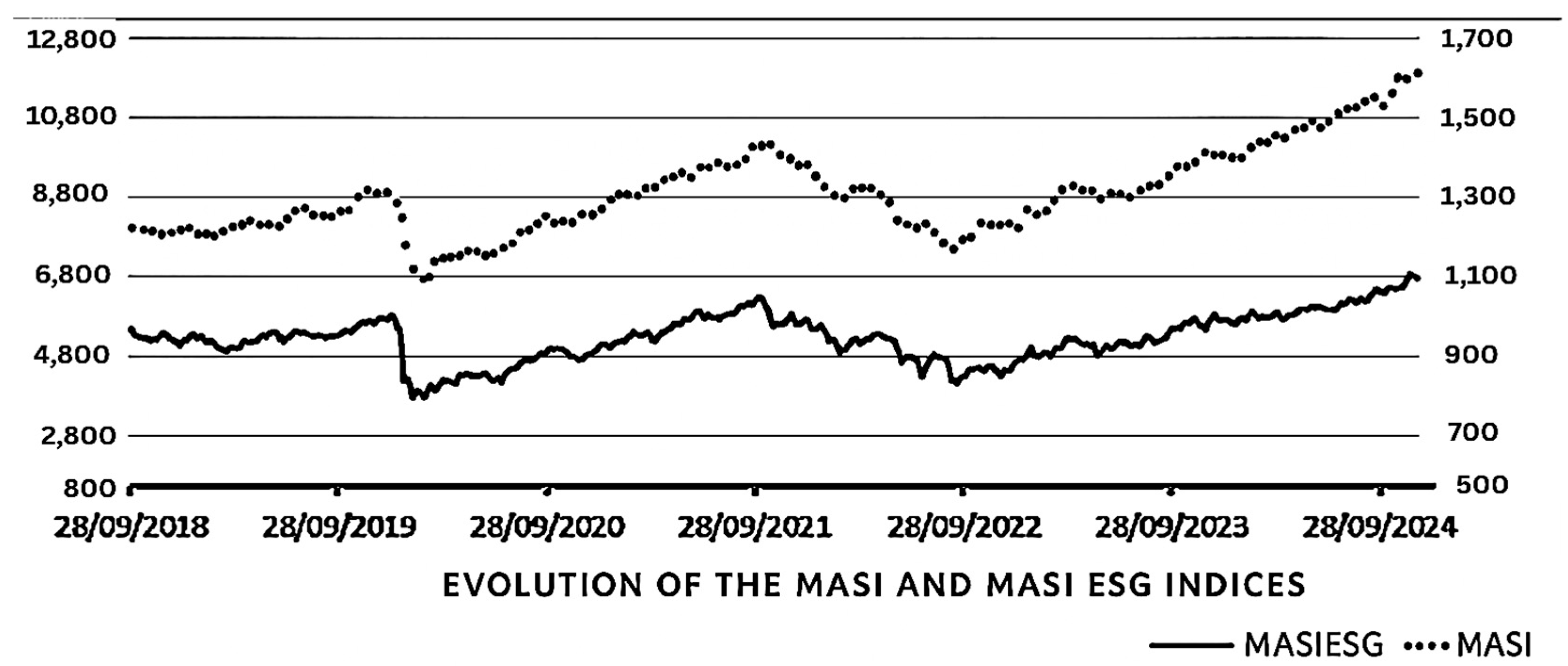
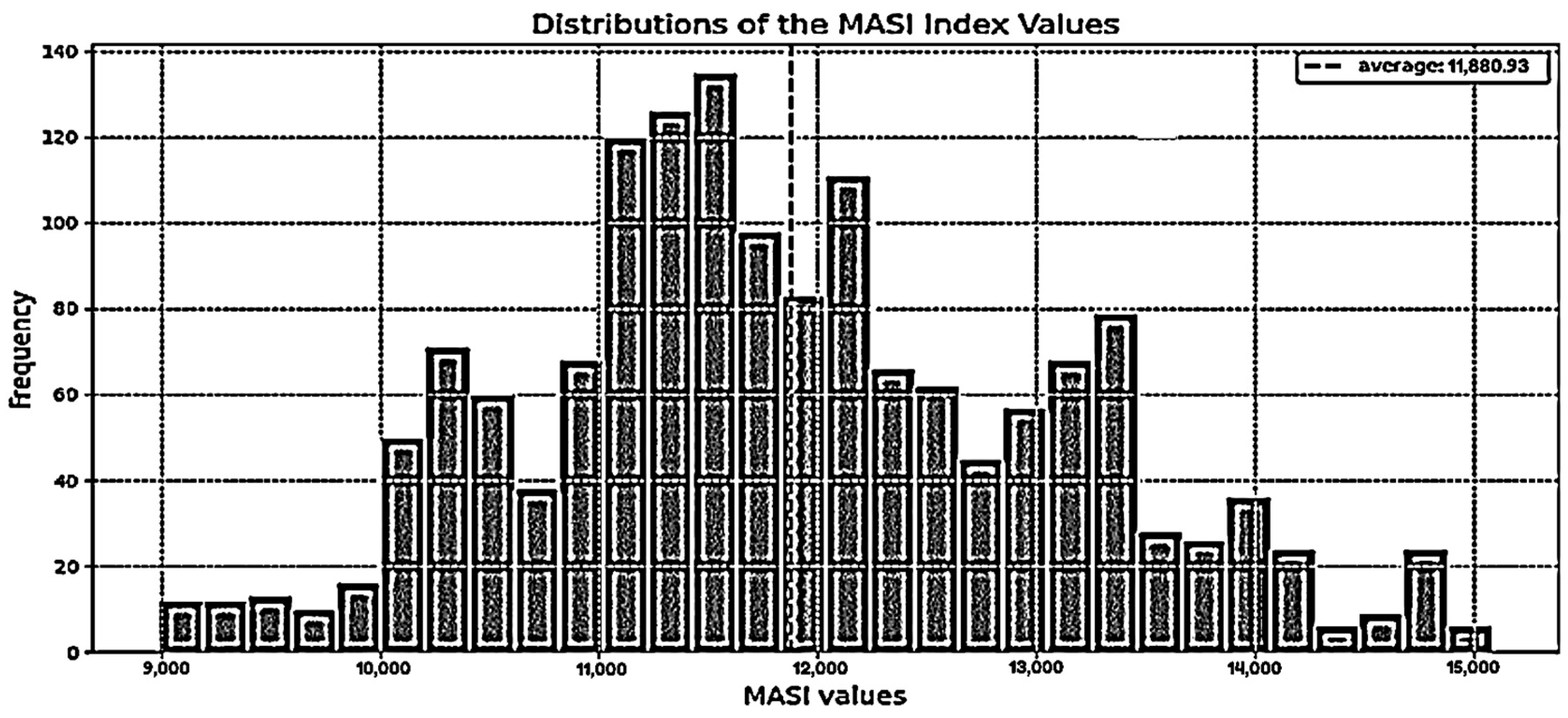
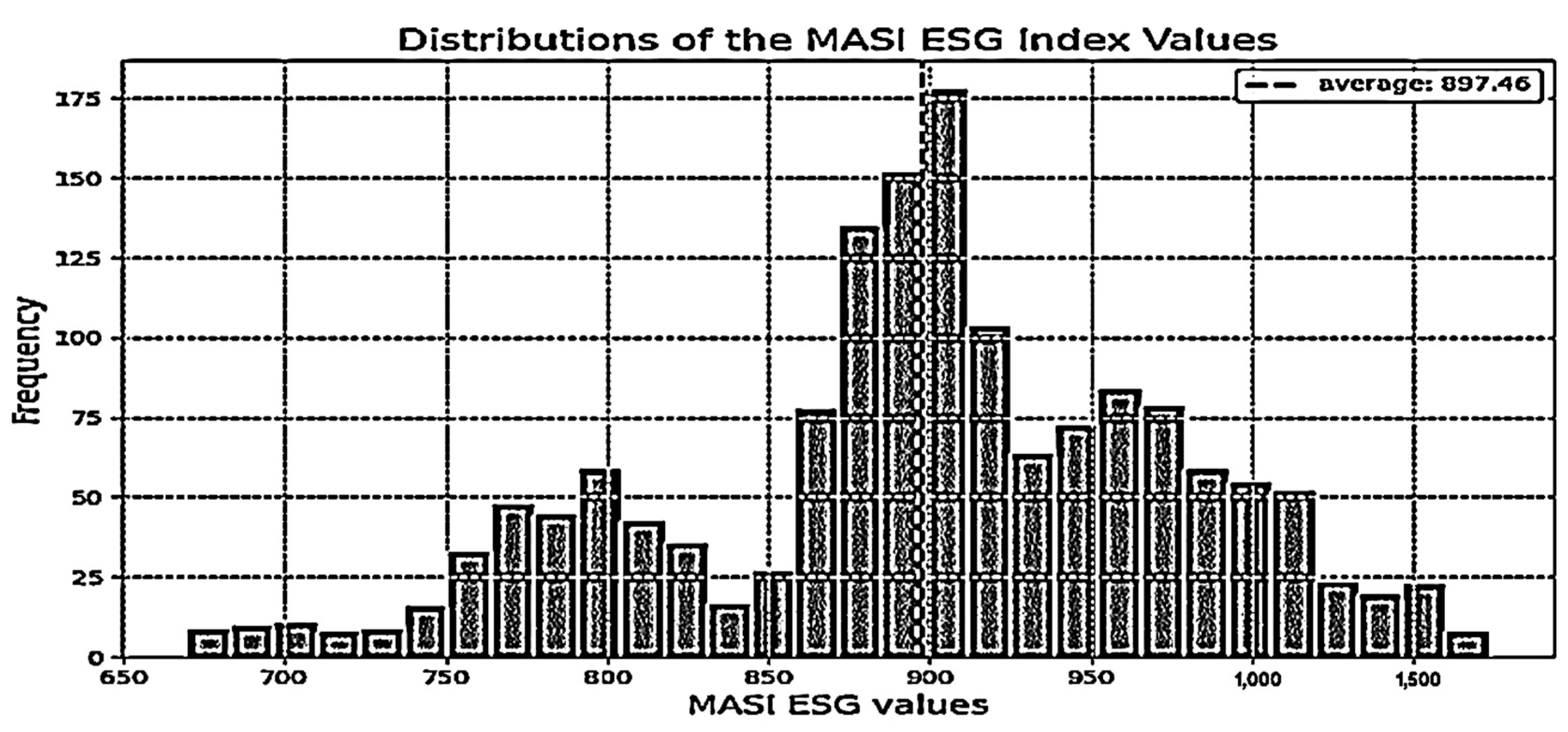
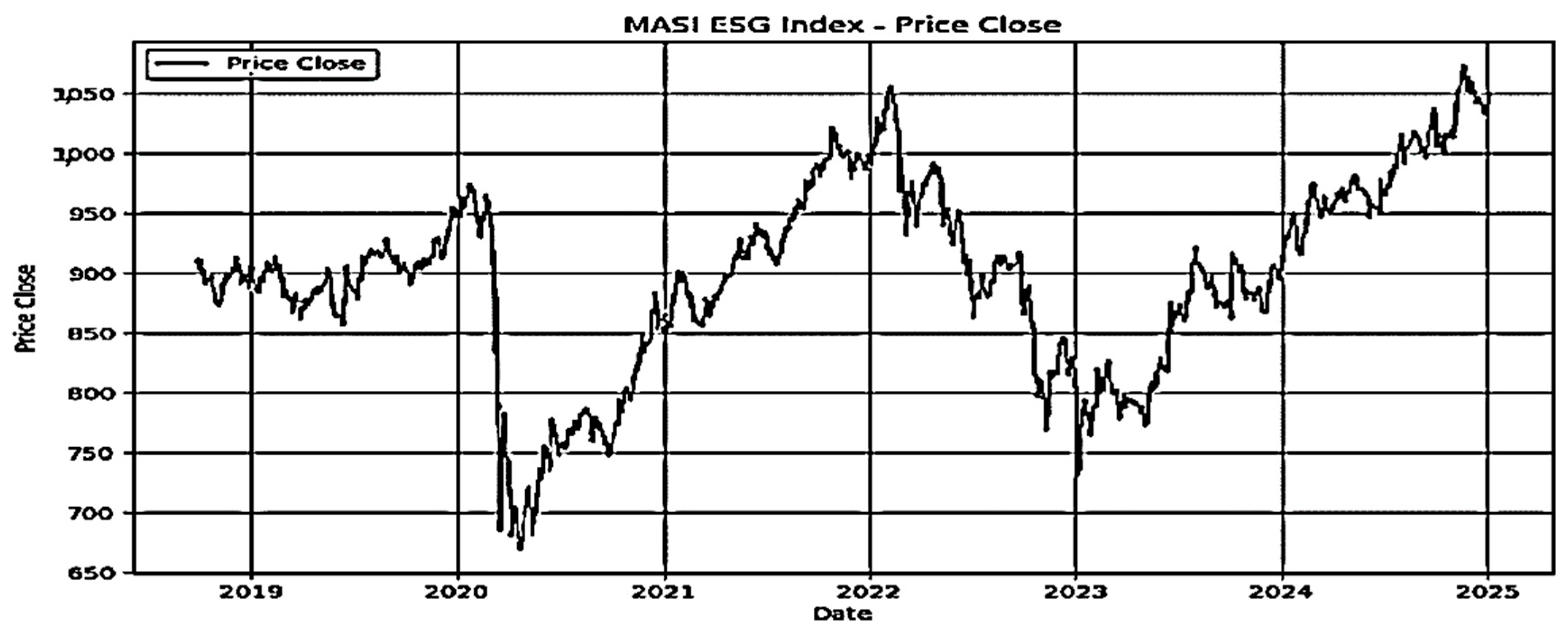
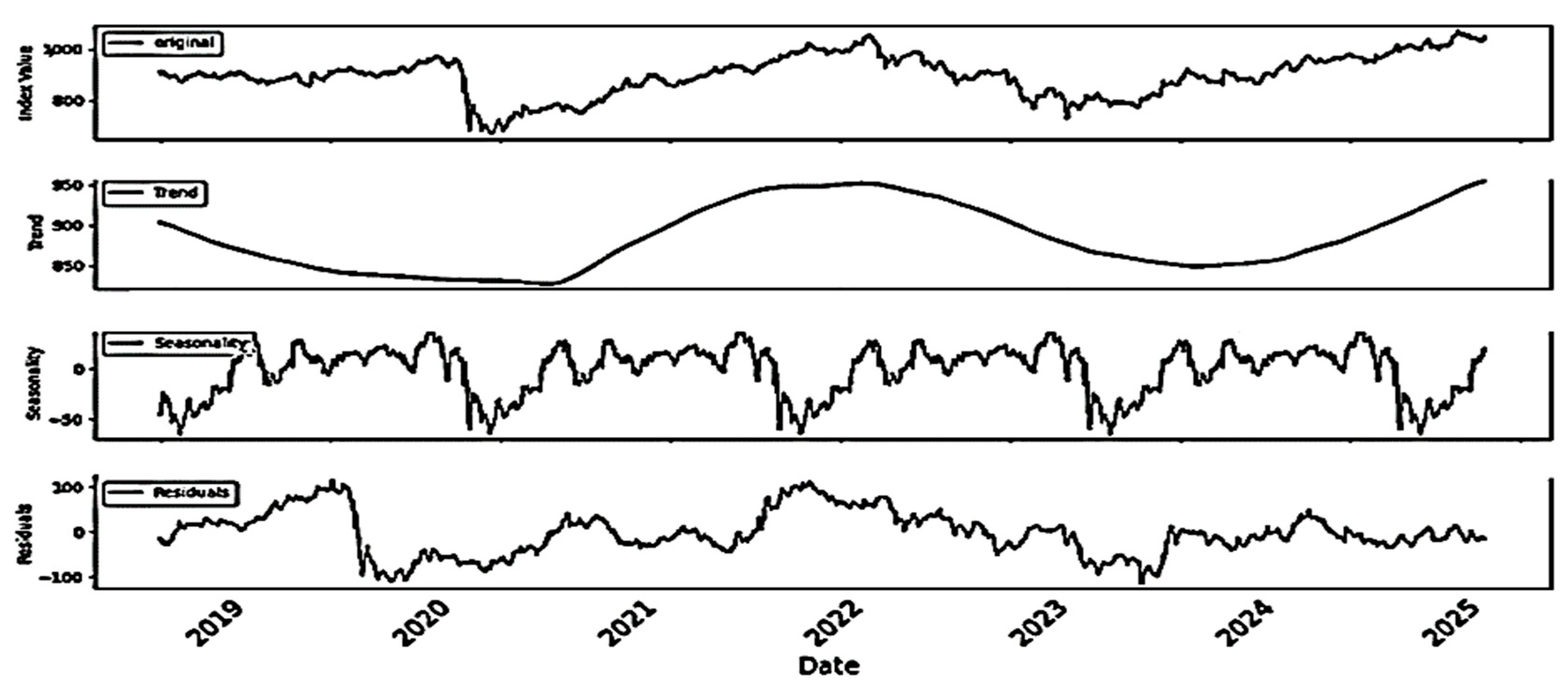
• Visualization of Time Series:

Figure 1, presented below, illustrates the evolution of the MASI and MASI ESG indices over the period from 28 September 2018 to 3 January 2025. This figure provides a clear visualization of the overall trends and the daily fluctuations observed in both indices, thereby offering insight into their respective market dynamics during the studied period.

The daily returns of the MASI and MASI ESG indices showed notable volatility, characterized by peaks occurring at specific periods. These peaks, typical of financial markets, may result from external economic or political events influencing the indices. One such period of heightened volatility occurred during the COVID-19 pandemic, which amplified market uncertainty due to the global health crisis and its economic ramifications. Volatility during this time was marked by extreme fluctuations in returns, both upwards and downwards. The average volatility of the MASI index returns is 0.101, while for the MASI ESG index, it is 0.066. These values reflect the intensity of fluctuations and the variability of the returns observed during the analysis period. This high volatility, relative to the average returns, highlights the short-term instability of the indices.

⮚

Average Returns:

The average daily returns of the MASI and MASI ESG indices are close to zero, with respective values of 0.000183509 and 9.11 × 10⁻⁵. These results are consistent with financial theory, which suggests that, over the long term, the returns of financial indices tend to fluctuate around zero. This indicates a relative stability of the indices in terms of average returns over short periods.

⮚

Volatility:

The daily volatility of the MASI and MASI ESG indices is 0.007620771 and 0.00855852, respectively. These values reflect the extent of variation in the indices’ returns over a given period. Generally, higher volatility signals greater uncertainty about future returns and may indicate relative market instability.

⮚

Skewness and Kurtosis Analysis of Return Distributions:

The analysis of skewness and kurtosis coefficients provides a better understanding of the shape of the return distributions for the MASI and MASI ESG indices. Figure 2 illustrates the skewness and kurtosis analysis of the return distributions for the MASI series. The skewness coefficient of −1.841 indicates a negatively skewed distribution, with a longer left tail than the right. This suggests a tendency for more frequent and extreme negative returns compared to positive returns, a phenomenon often observed in response to unfavorable events such as economic crises or political shocks. Furthermore, the kurtosis coefficient highlights thick tails in the distribution, suggesting a non-normal distribution. In other words, extreme returns (both positive and negative) occur more frequently than in a normal distribution.

Figure 3 presents the skewness and kurtosis analysis of the return distributions for the MASI ESG series. The skewness coefficient of −1.574 also indicates a negative skew, though slightly less pronounced than the MASI index. Similar to the MASI series, the kurtosis coefficient for the MASI ESG index suggests the presence of thick tails in the distribution, further supporting the notion that extreme events, although rare, can lead to sharp and significant movements in the indices.

This characteristic is common in financial markets, where extreme events, despite their rarity, can lead to significant and often unpredictable movements in the indices.

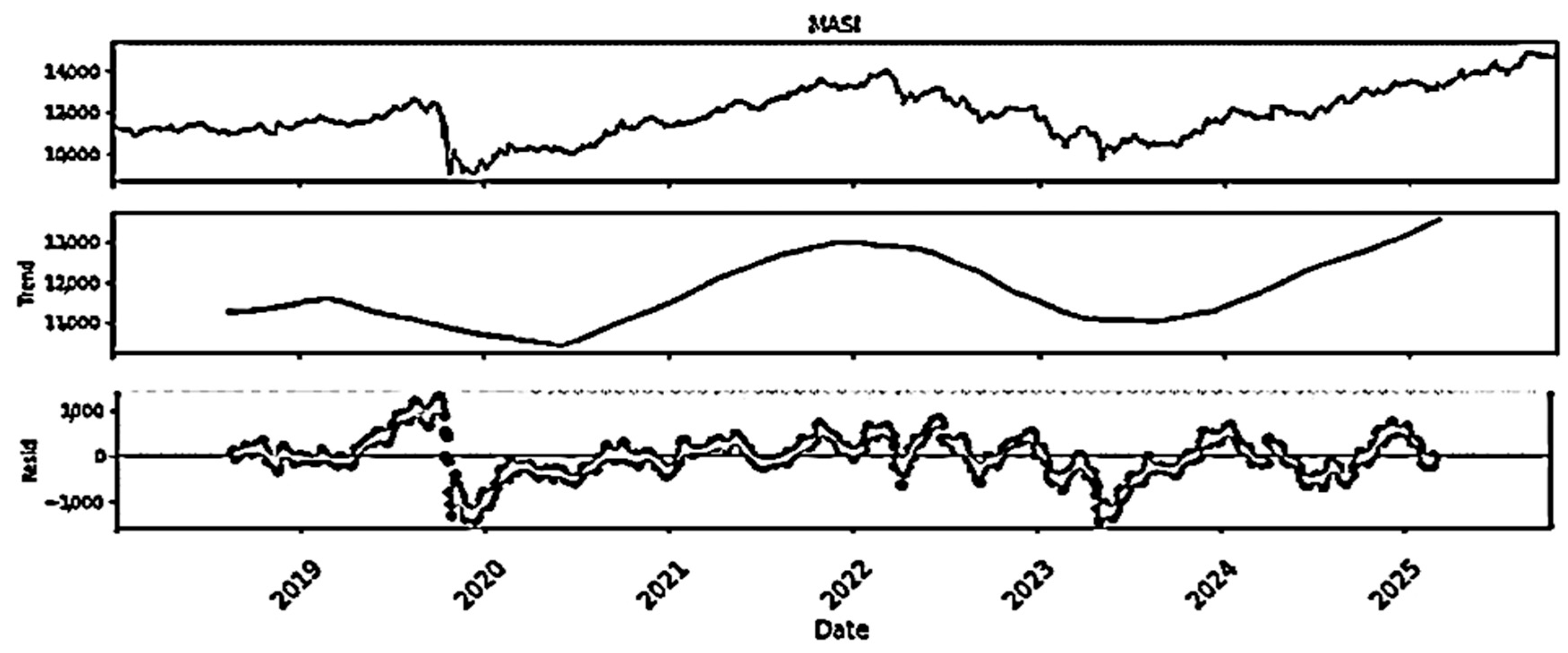
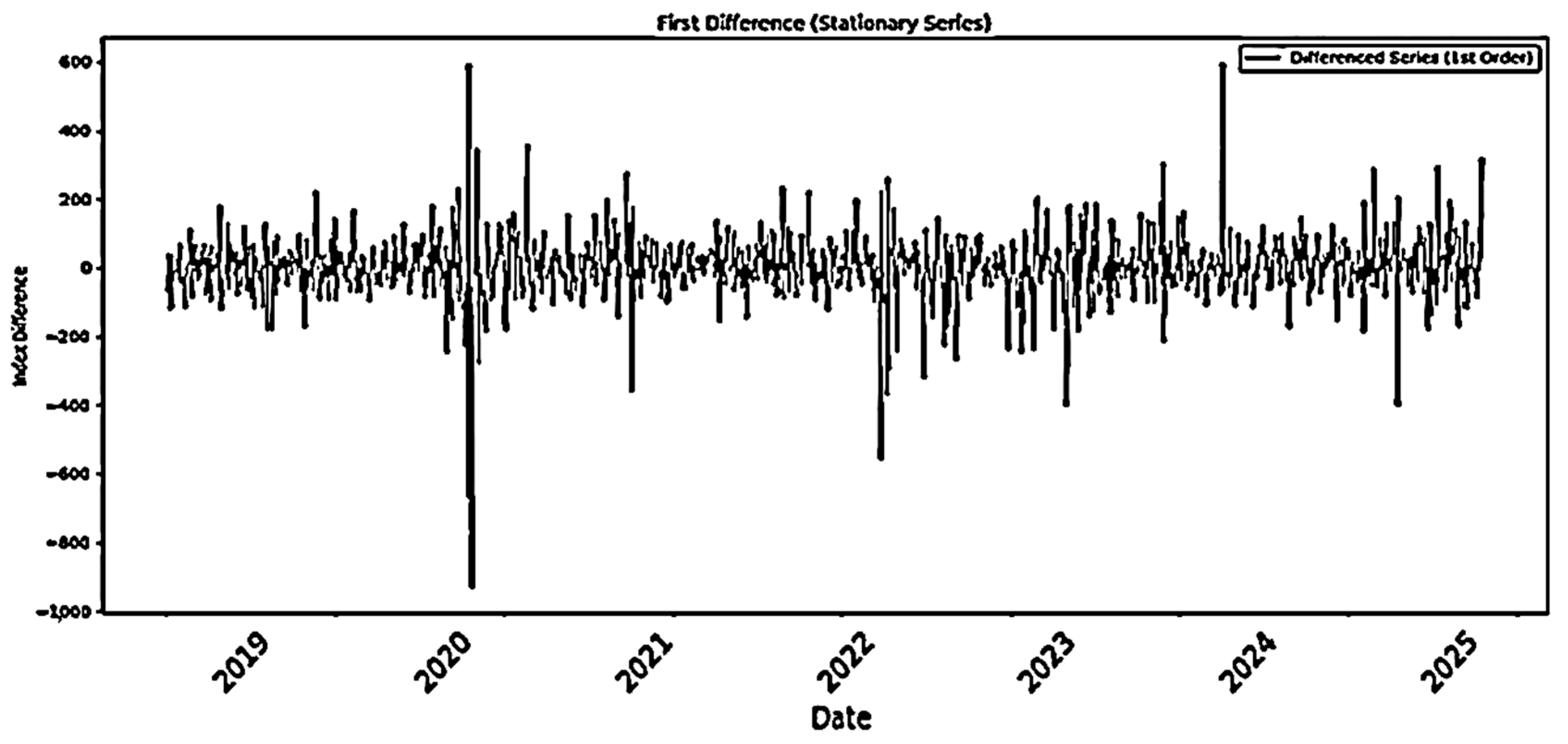
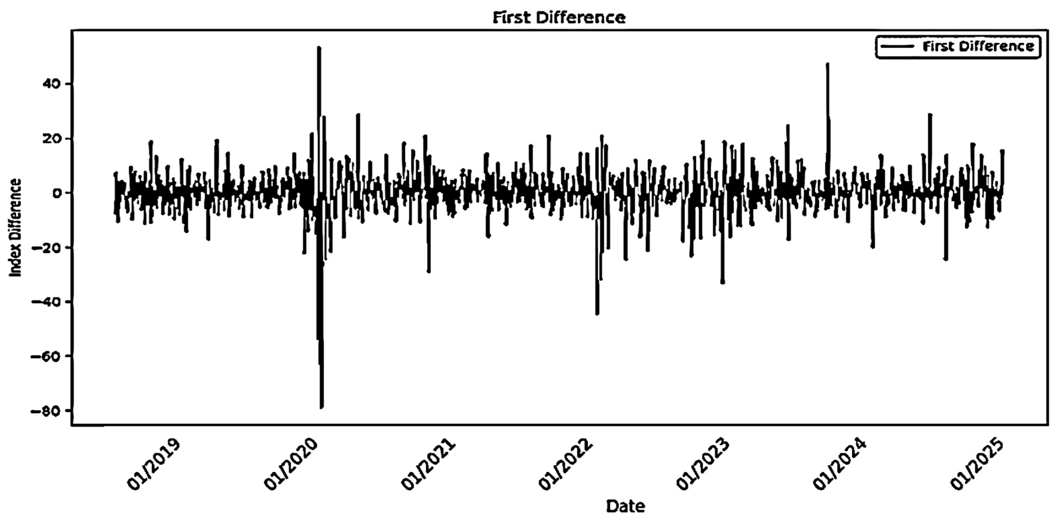
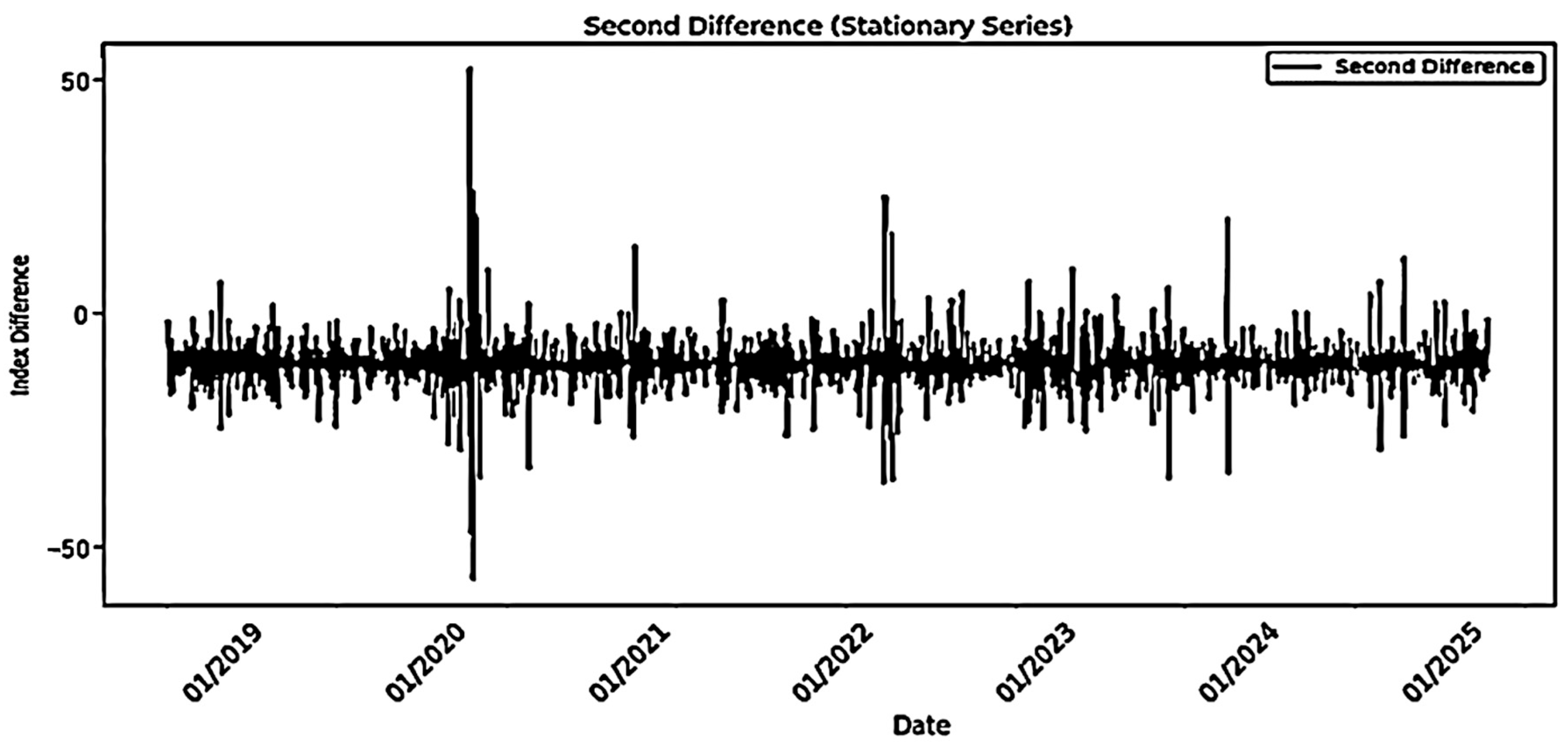
3.2.2. Stationarity Assessment and Differencing of MASI and MASI ESG Indices

• Stationarity Analysis: Application of ADF, KPSS, PP, and Zivot–Andrews Tests:

The Augmented Dickey–Fuller (ADF) test is commonly used to detect stationarity. In this study, the MASI and MASI ESG indices were first subjected to the ADF test, which indicated that both series were non-stationary. The non-stationarity of the MASI ESG index was attributed to trends and seasonality, while the non-stationarity of the MASI index was primarily due to a trend.

Stationarizing the time series for the MASI and MASI ESG indices was a crucial step in preparing the data for analysis. The primary goal was to make these series stationary, allowing them to be used in forecasting models that assume stable behavior of the data over time. Stationarity tests (ADF, KPSS, PP, and Zivot–Andrews) revealed that both series exhibited trends and non-stationary characteristics. Consequently, differencing was applied to eliminate these effects and render the series stationary. Once the series were made stationary, the models were able to generate more reliable forecasts, leading to a better understanding of the future dynamics of the indices.

⮚

Stationarity of the MASI Index

Table 1. MASI index.

Variable	ADF Test	KPSS Test	Phillips–Perron Test	Zivot–Andrews Test	Order of Integration
MASI	ADF: −9.5345 p-value: 2.83 × 10−16	KPSS: 0.1582 p-value: 0.0152	PP: −9.8457 p-value: 1.56 × 10−16	ZA: −10.2235 p-value: 1.08 × 10−15	I(1)

below presents the stationarity test results for the MASI index, both before and after differencing. To render the series stationary, differencing was applied, which effectively removed the overall trend. After stationarization, the daily returns of the MASI index became erratic and showed no particular direction. A second round of ADF, KPSS, PP and Zivot_Andrews tests con-firmed that the series was now stationary, making it suitable for use in classical statistical models like ARIMA and GARCH for analyzing and forecasting returns.

⮚

Stationarity of the MASI ESG Index

Table 2. MASI ESG index.

Variable	ADF Test	KPSS Test	Phillips–Perron Test	Zivot–Andrews Test	Order of Integration
MASI ESG	ADF: −8.55 p-value: 0.1143	KPSS: 0.1181 p-value: 0.1862	PP: −8.5422 p-value: 0.1326	ZA: −8.8210 p-value: 0.1598	I(1)
	ADF: −13.6389 p-value: 1.67 × 10−25	KPSS: 0.0653 p-value: 0.1862	PP: −13.5374 p-value: 0.0214	ZA: −13.6458 p-value: 0.0002	I(2)

below presents the stationarity test results for the MASI ESG index, both before and after differencing. The MASI ESG index, which integrates environmental, social, and governance (ESG) criteria, initially exhibited non-stationary characteristics, as revealed by the ADF, KPSS, PP, and Zivot_Andrews tests. This non-stationarity was attributed to the presence of long-term trends and potential seasonal variations influenced by ESG-related factors. To render the series stationary, a second-order differencing was applied, which successfully eliminated the trend and stabilized the variance. A second round of stationarity tests confirmed that the series had become stationary, making it appropriate for analysis and forecasting using classical models such as ARIMA and GARCH.

The Kwiatkowski–Phillips–Schmidt–Shin (KPSS) test and the Phillips–Perron (PP) test were applied. The KPSS test confirmed the stationarity of the series around a deterministic trend, while the PP test provided further confirmation of stationarity, particularly in cases with potential heteroscedasticity and autocorrelation.

Additionally, the Zivot–Andrews test was performed to test for stationarity while accounting for potential structural breaks in the time series. This test is particularly relevant when significant changes in the data may affect stationarity. Conducting multiple stationarity tests increases the robustness of the results, particularly by considering different aspects of the time series (trend, seasonality, breaks).

While differencing was applied to both indices to achieve stationarity, the ADF test revealed that the first-order differencing for the MASI ESG index was not statistically significant, meaning it did not adequately remove the trend or seasonality in the data. In contrast, the second-order differencing yielded a significant result, indicating that the series became stationary at this order. This confirms that the MASI ESG index has a more complex trend or potential seasonal component that requires two differences to stabilize the series effectively. Therefore, we chose to apply the second-order differencing to the MASI ESG index to ensure the data met the stationarity requirement for classical forecasting models.

3.2.3. Graphical Validation of Differentiation

To ensure the suitability of the data for classical forecasting models, both the MASI and MASI ESG indices were examined for stationarity. Initially, the MASI index exhibited a clear upward trend and a non-constant mean, as illustrated in Figure 4: The MASI index before differencing. Further inspection revealed the origin of non-stationarity, as shown in Figure 5: Source of non-stationarity of the MASI index. After applying a first-order differencing, the series showed no discernible trend and fluctuated randomly around a constant mean, as seen in Figure 6: Series MASI after first differencing.

Similarly, the MASI ESG index displayed non-stationary behavior in its original form, with long-term trends depicted in Figure 7: The MASI ESG index before differencing and Figure 8: Source of non-stationarity of the MASI ESG index. A first-order differencing partially corrected the trend (Figure 9: Series MASI ESG after first differencing), but it was only after applying a second-order differencing that full stationarity was achieved, as illustrated in Figure 10: Series MASI ESG after second differencing.

After differencing, the graphs revealed more erratic series, where the values oscillated around zero without any clear direction. The absence of any apparent trend and the stability of fluctuations confirmed that the series were now stationary. These transformations allowed the data to meet the prerequisites for time series modeling and justified the use of classical forecasting techniques such as the ARIMA and GARCH models.

• Implications of Stationarity for Analysis:

The stationarity of the series has been crucial for the validity of the analysis. A stationary index is essential for statistical modeling because it ensures that the statistical properties of the series remain constant over time. By making the return series of the MASI and MASI ESG indices stationary, it was possible to ensure that the results of forecasting models, such as the ARIMA, SARIMA, and GARCH models, would be reliable. These transformations also had a significant impact on the interpretation of underlying economic and financial relationships. For example, by making the daily returns of the indices stationary, it became possible to analyze the relationships between past and future returns, fluctuations in volatility, and the potential impact of different exogenous factors on the performance of stock indices.

4. Empirical Results

4.1. Forecasting Returns

The forecasting of returns for the MASI and MASI ESG indices is essential for both risk management and investment decision-making. To achieve accurate predictions, the ARIMA and SARIMA models were employed. These models proved to be highly effective in forecasting the average returns of both indices, capturing key trends and fluctuations over a period of 252 trading days, approximately one year.

For the MASI index, the ARIMA model was applied after differencing the time series to ensure stationarity. The optimal parameters for the ARIMA model (p, d, q) were selected using the Akaike Information Criterion (AIC), a widely used method for model evaluation that balances fit and complexity. The forecasts for the MASI index indicated returns close to zero, with slight variations over time. These predictions remained stable, aligning well with the historical dynamics of the index. The ARIMA model effectively captured past behaviors, providing reliable forecasts of future returns.

For the MASI ESG index, the forecasting process involved a hybrid approach combining both the ARIMA and SARIMA models. While the ARIMA model addressed the overall trend, the SARIMA model incorporated seasonal effects into the forecasts. SARIMA, which includes additional seasonal parameters (P, D, Q, m), was particularly useful for accounting for the recurring seasonal fluctuations observed in the MASI ESG index. The inclusion of seasonal components improved the accuracy of the forecasts, as it allowed the model to better reflect the index’s cyclical behavior over time. This approach enhanced the predictive power, capturing both the general trends and the seasonality inherent in the MASI ESG returns.

Together, the ARIMA and SARIMA models demonstrated strong robustness in forecasting returns for both indices. While the ARIMA model provided a reliable prediction for the MASI index, the SARIMA model, by factoring in seasonal patterns, proved particularly effective for the MASI ESG index, highlighting the importance of incorporating seasonality in financial time series analysis.

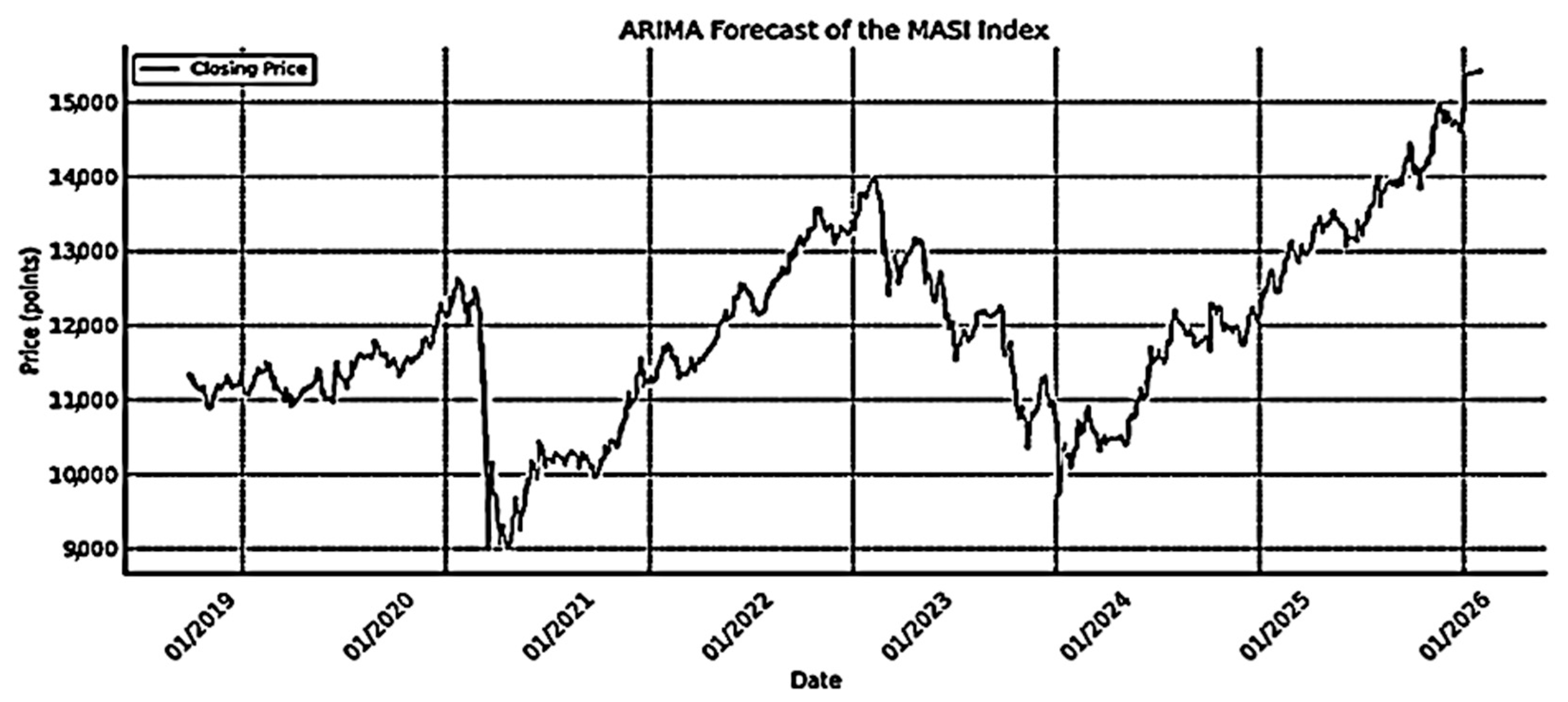
4.1.1. Return Forecasts (ARIMA and SARIMA)

The graph depicts the expected evolution of average returns over the 252 trading days for the MASI and MASI ESG indices, along with confidence intervals for the forecasts.

Figure 11: MASI index return forecast by ARIMA model illustrates the evolution and forecast of the MASI index closing price, expressed in points, over the period from January 2019 to January 2026 using an ARIMA model (AutoRegressive Integrated Moving Average). The chart reveals a non-stationary time series characterized by significant volatility, including a sharp drop at the end of 2020, followed by a strong recovery and a sustained upward trend from 2023 onward. The ARIMA model, by capturing the autoregressive, differencing, and moving average components, effectively models the underlying dynamics of the index and projects its future trajectory. The anticipated upward trend through 2026 reflects a structural market recovery, indicating systemic resilience and a favorable outlook from economic agents regarding medium-term macro-financial stability.

Figure 12: MASI ESG index return forecast by ARIMA model presents the historical evolution and forecast of the MASI ESG Index closing price, measured in points, from January 2019 to January 2026, using an ARIMA (AutoRegressive Integrated Moving Average) model. The time series reveals a pronounced non-stationarity with evident periods of volatility, including a steep decline in late 2020, indicative of an exogenous shock, followed by a gradual and robust recovery. The ARIMA model captures the autoregressive dependencies, integrated trends, and moving average effects within the data, allowing for a statistically grounded forecast of future index movements. From early 2022 onward, the index demonstrates a clear upward trend, with projected growth continuing through 2026. This trajectory reflects a strengthening of ESG-compliant investments, suggesting increasing investor confidence in sustainable assets and reinforcing the structural resilience and positive outlook of ESG-oriented market segments over the medium term.

Figure 13: Forecasting the returns of the MASI ESG index using the SARIMA model depicts the historical behavior and forecast of the MASI ESG Index closing price, expressed in points, from January 2019 to January 2026, employing a SARIMA (Seasonal AutoRegressive Integrated Moving Average) model. The time series displays clear non-stationary characteristics with both trend and seasonal components, alongside significant volatility. A sharp downturn is observed around late 2020, followed by a steady recovery and a cyclical pattern of fluctuations. The SARIMA model enhances the traditional ARIMA approach by integrating seasonal differencing, which captures periodic behaviors and repeating patterns in the data. The forecast reveals a stable upward trend from 2023 onward, indicating not only a long-term structural rebound but also the persistence of seasonal effects in ESG investment performance. This model-based projection underlines the resilience and growing investor alignment with sustainability principles, affirming the robustness of ESG indices in the face of market shocks and their favorable outlook in the medium-to-long term.

4.1.2. Regression Coefficients for ARIMA and SARIMA Models of MASI and MASI ESG Indices

The regression results for the ARIMA and SARIMA models indicate that both indices exhibit statistically significant autoregressive and moving average components, suggesting that their returns are influenced by past values and forecast errors. The MASI ESG index required a second differencing, indicating it is less stationary and more volatile over time compared to the MASI index. Incorporating seasonality through the SARIMA model improved the model fit for the MASI ESG index, highlighting the presence of seasonal patterns in its behavior.

Table 3. MASI—ARIMA (1st differencing).

Model	(p,d,q)	Coefficients	Std. Error	t-Stat	p-Value	AIC
ARIMA	(1,1,1)	AR(1) = 0.45	0.12	3.75	0.0002	−1125
		MA(1) = −0.38	0.10	−3.80	0.0001

: MASI—ARIMA (1st differencing) presents the estimation results for the ARIMA(1,1,1) model applied to the MASI index. The autoregressive coefficient AR(1) is estimated at 0.45 with a standard error of 0.12, yielding a t-statistic of 3.75 and a highly significant p-value of 0.0002, indicating a strong positive influence of the previous period’s value on the current return. Similarly, the moving average coefficient MA(1) is estimated at −0.38 (standard error 0.10, t-statistic −3.80, p-value 0.0001), showing a significant correction based on past forecast errors. The model achieves a low Akaike Information Criterion (AIC) value of −1125, suggesting a good fit. These statistically significant parameters confirm that the MASI index returns are both autocorrelated and influenced by prior disturbances, supporting the appropriateness of the ARIMA(1,1,1) specification.

Table 4. MASI ESG—ARIMA (2nd differencing).

Model	(p,d,q)	Coefficients	Std. Error	t-Stat	p-Value	AIC
ARIMA	(1,2,1)	AR(1) = 0.52	0.14	3.71	0.0003	−980
		MA(1) = −0.47	0.13	−3.62	0.0004

: MASI ESG—ARIMA (2nd differencing) displays the estimation results of the ARIMA(1,2,1) model applied to the MASI ESG index. The autoregressive coefficient AR(1) is estimated at 0.52 with a standard error of 0.14, producing a t-statistic of 3.71 and a highly significant p-value of 0.0003, indicating that past values significantly influence current returns even after two levels of differencing. The moving average coefficient MA(1) is estimated at −0.47 (standard error 0.13, t-statistic −3.62, p-value 0.0004), also statistically significant, reflecting the model’s correction based on past forecast errors. The need for a second differencing (d = 2) suggests that the MASI ESG index is less stationary and exhibits greater long-term volatility than the standard MASI index. Despite a slightly higher AIC value of −980, the model still provides a reasonably good fit. These results underscore the importance of both autoregressive and error–correction dynamics in capturing the behavior of ESG-aligned investments, which tend to react more sensitively to structural and external market shifts.

Table 5. MASI ESG—SARIMA (2nd differencing + seasonality).

Model	(p,d,q)(P,D,Q)m	Coefficients	Std. Error	t-Stat	p-Value	AIC
SARIMA	(1,2,1)(0,1,1)[12]	AR(1) = 0.49	0.11	4.45	0.00001	−1038
		MA(1) = −0.41	0.09	−4.55	0.00000
		SMA(1) = −0.36	0.08	−4.50	0.00000

: MASI ESG—SARIMA (2nd differencing + seasonality) presents the results from the SARIMA(1,2,1)(0,1,1) [12] model, which incorporates both non-seasonal and seasonal dynamics to better capture the behavior of the MASI ESG index. The autoregressive coefficient AR(1) is estimated at 0.49 (standard error 0.11, t-stat = 4.45, p-value = 0.00001), indicating a significant dependence on past values. The moving average term MA(1) is −0.41 (standard error 0.09, t-stat = −4.55, p-value = 0.00000), showing a strong correction based on prior errors. Crucially, the seasonal moving average component SMA(1) is −0.36 (standard error 0.08, t-stat = −4.50, p-value = 0.00000), capturing statistically significant seasonal patterns with a periodicity of 12 months. The AIC of −1038 represents a substantial improvement over the non-seasonal ARIMA model (AIC = −980), indicating a superior model fit. These findings confirm the presence of both short-term autocorrelations and seasonal dependencies in the ESG index returns, reinforcing the added value of seasonal modeling when analyzing the dynamic behavior of sustainable financial assets.

These regression results for the ARIMA and SARIMA models confirm the significant role of autoregressive and moving average components in both indices’ returns. The MASI ESG index required a second differencing due to its higher volatility and less stationary nature, while the incorporation of seasonal effects via the SARIMA model improved the fit for the MASI ESG index.

4.2. Volatility Forecasting

Volatility forecasting for the MASI and MASI ESG indices was conducted using the ARCH, GARCH, EGARCH, and GJR-GARCH models, all of which proved effective in providing reliable estimates of conditional volatility. The ARCH model, designed to model time-varying volatility, allows the variance of returns to change based on past values, making it particularly useful for analyzing volatility during periods of instability. However, its limitations include reduced efficiency over long time series and an inability to capture long-memory effects in volatility dynamics. The GARCH model enhanced this approach by effectively capturing both high-volatility periods and calmer market conditions, showing how volatility evolved over time. The EGARCH model further refined the analysis by accounting for asymmetric volatility effects, with larger spikes following negative shocks, reflecting common financial market behavior, where bad news triggers more significant market reactions than good news. Similarly, the GJR-GARCH model highlighted the leverage effect, showing that negative shocks lead to larger increases in volatility compared to positive shocks, which is a typical feature of financial markets, where market participants tend to react more strongly to adverse information. Together, these models provided a comprehensive view of volatility dynamics, helping to better understand how market events impact the MASI and MASI ESG indices over time.

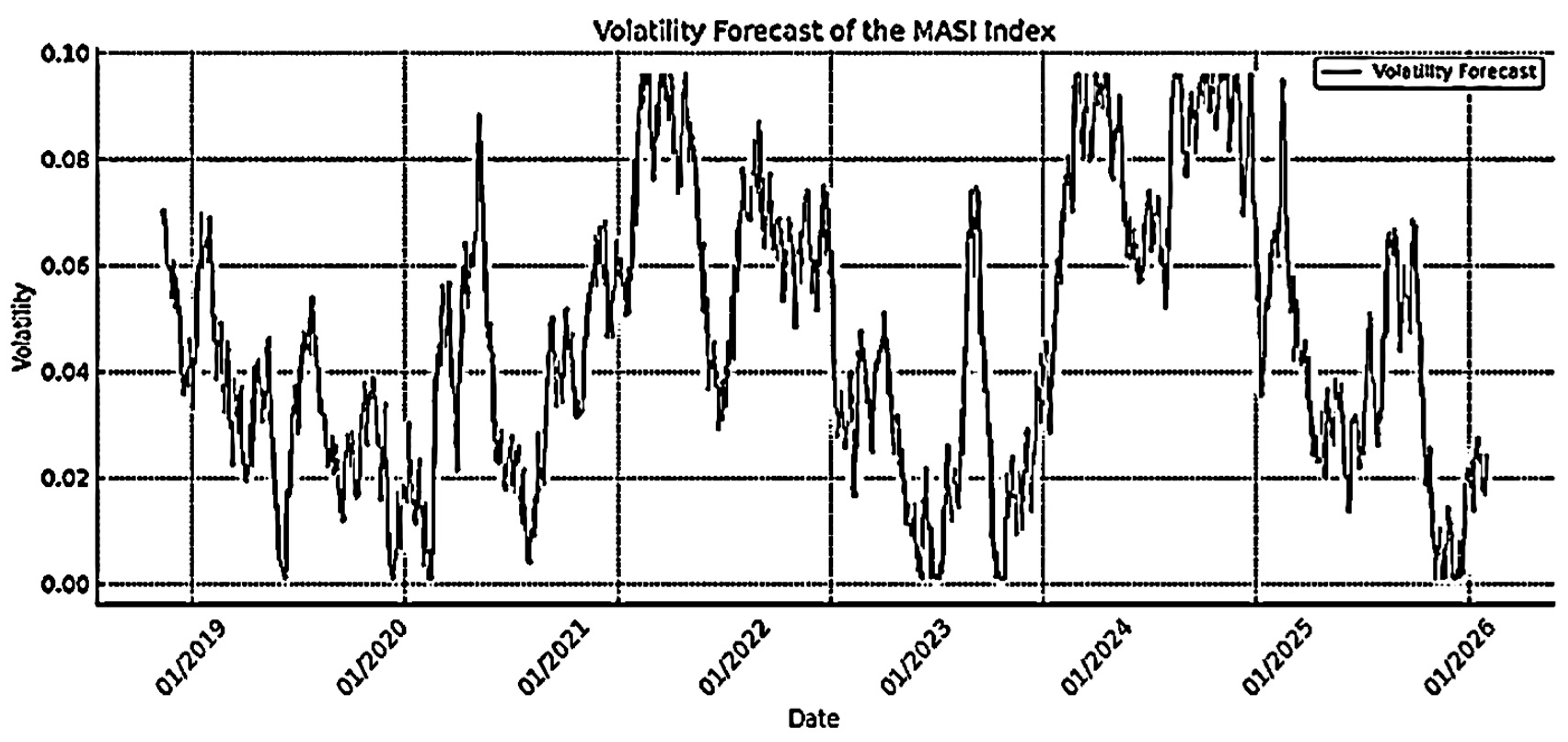
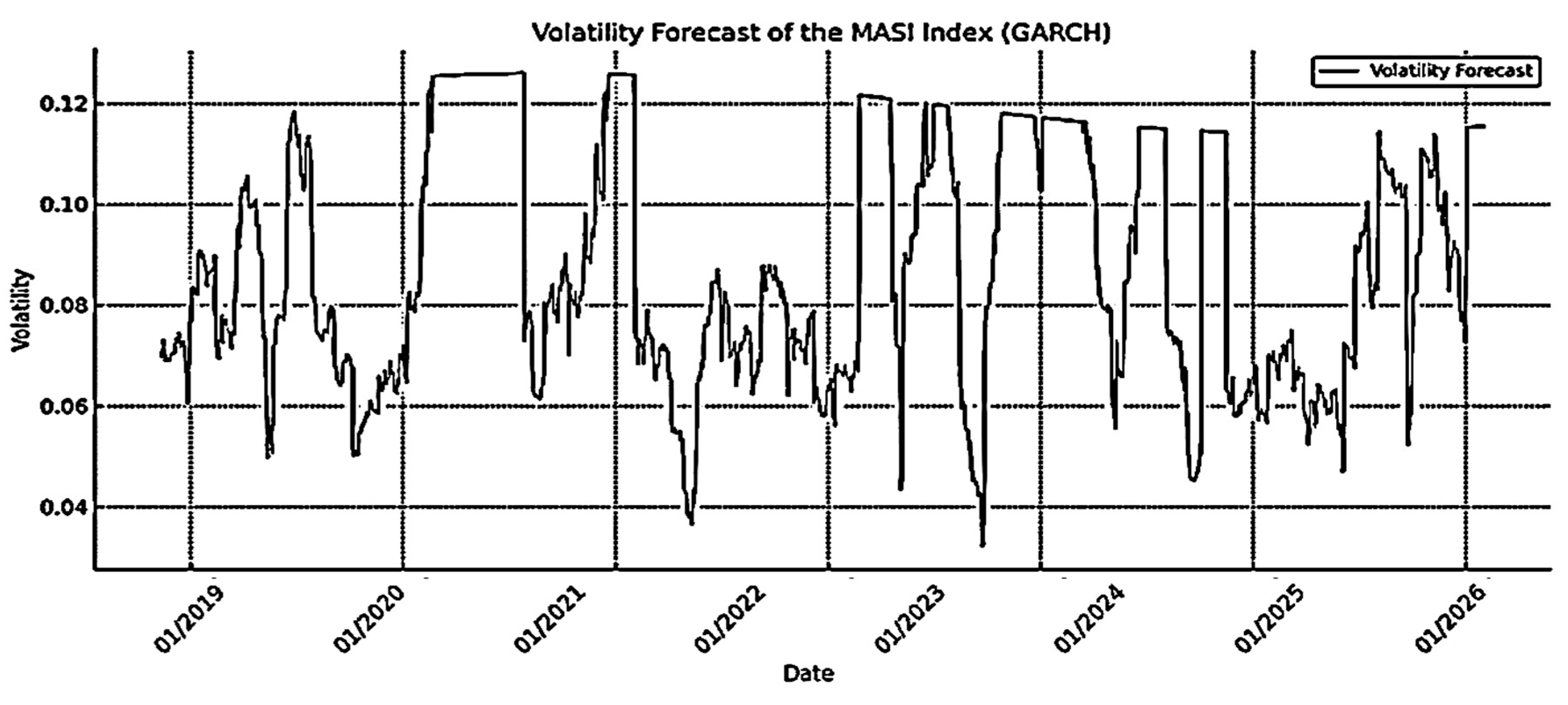
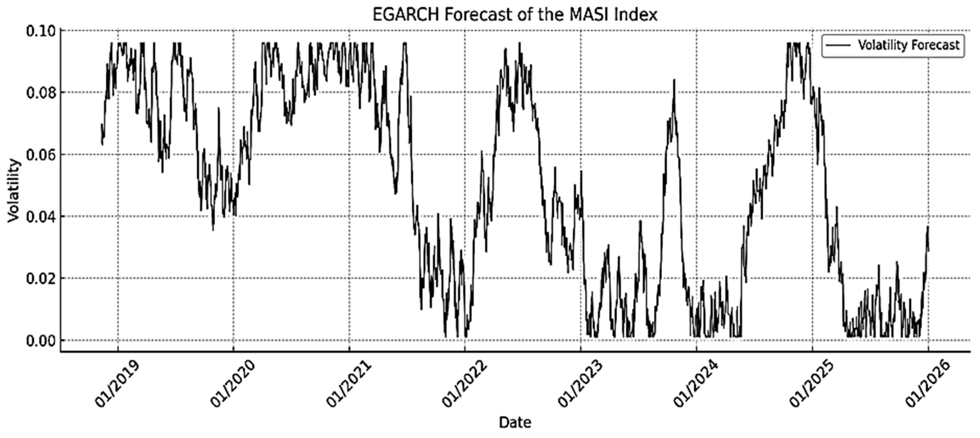
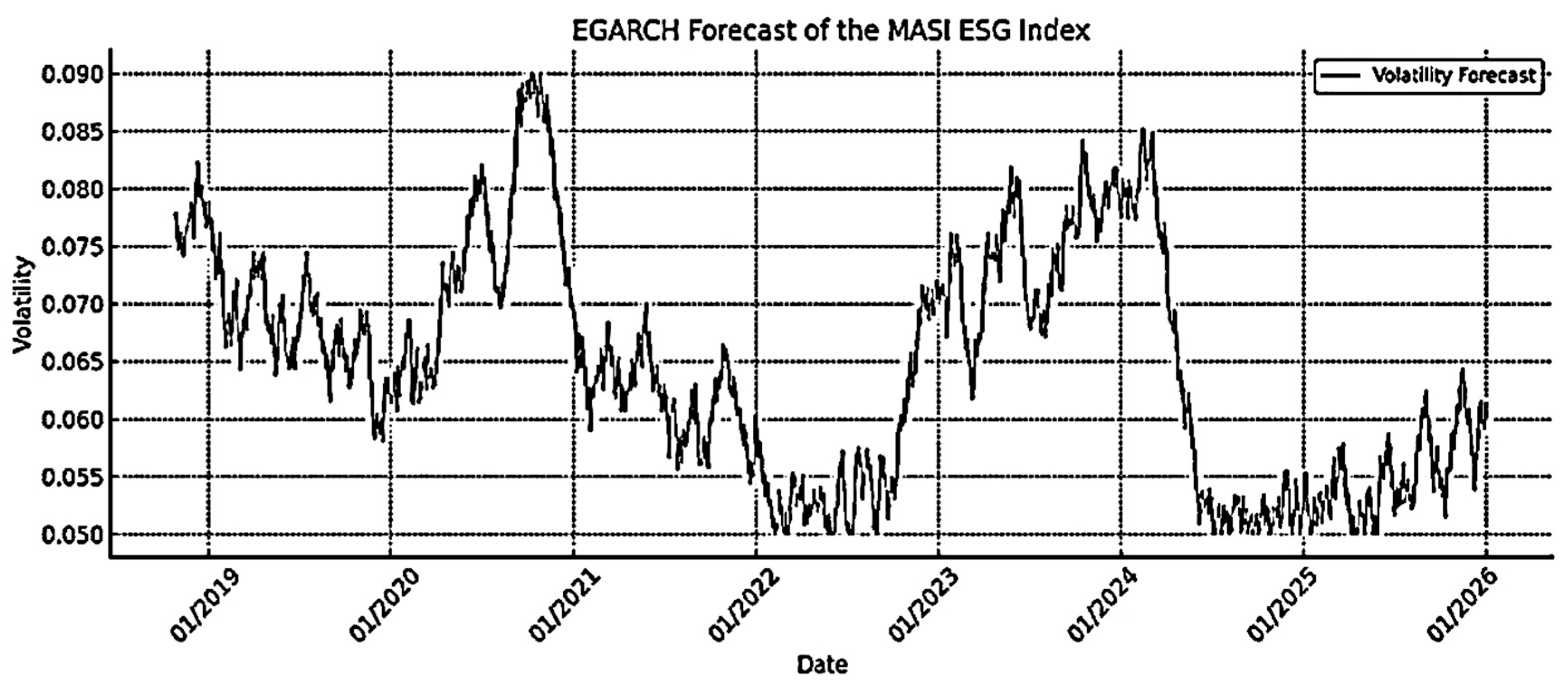
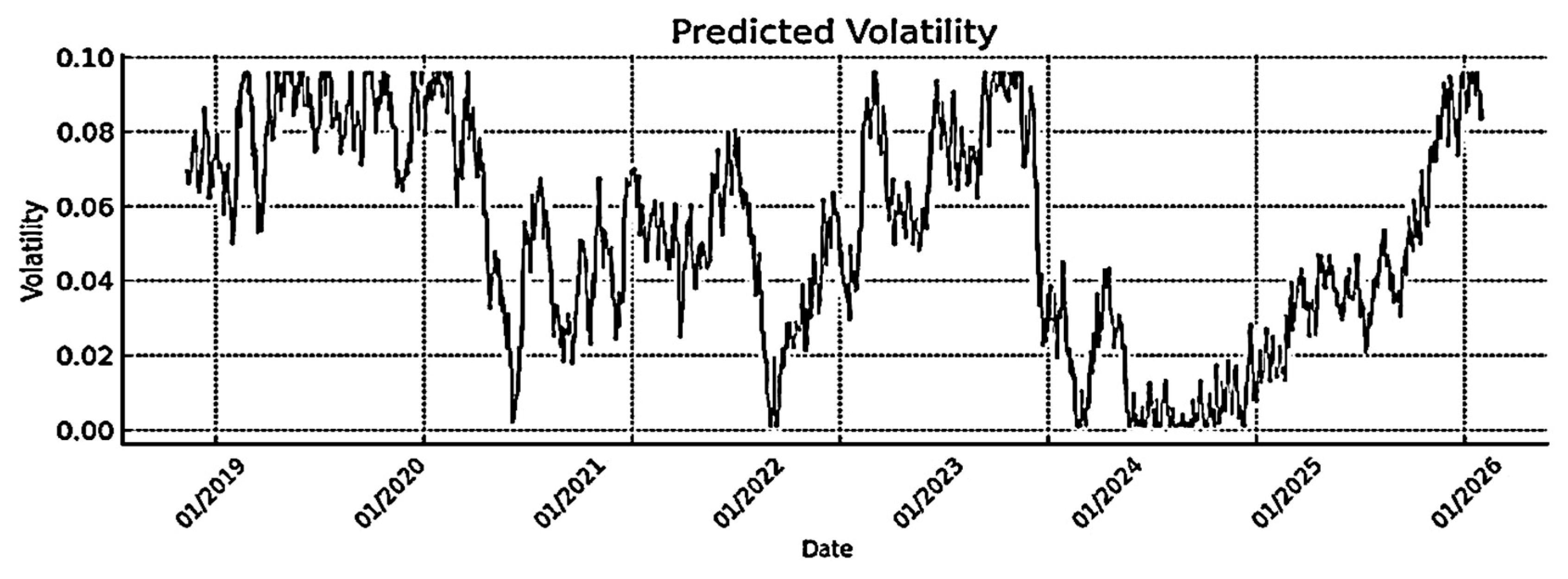
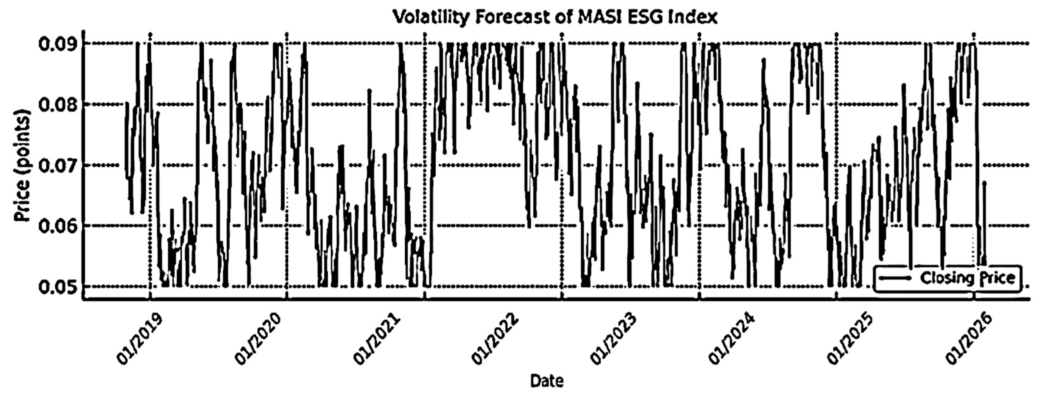
4.2.1. Volatility Forecasts (ARCH, GARCH, EGARCH, and GJR-GARCH)

The following graphs show the volatility forecasts for the MASI and MASI ESG indices, with seasonal variations and volatility spikes depending on positive or negative shocks.

Figure 14 presents the dynamic forecasts of the conditional volatility of the MASI Index over the period from January 2019 to January 2026, obtained using the ARCH (Autoregressive Conditional Heteroskedasticity) model, which is well known for its ability to model short-term conditional heteroskedasticity typical of financial time series. The results reveal significant volatility clustering, marked by pronounced spikes around early 2021, late 2023, and early 2024, possibly linked to macroeconomic or political shocks. In contrast, periods of relative calm, particularly in 2020 and at the end of 2025, reflect temporary market stability. These forecasts highlight the persistence of risk and suggest the presence of recurring or seasonal structural dynamics in the Moroccan stock market. Ultimately, the ARCH model enhances understanding of the MASI Index’s sensitivity to economic fluctuations, underscoring the importance of adaptive risk assessment tools for portfolio managers, financial analysts, and policymakers.

Figure 15 presents the projected conditional volatility of the MASI ESG Index from January 2019 to January 2026, based on the ARCH (Autoregressive Conditional Heteroskedasticity) model, which effectively captures the evolving nature of financial volatility. The forecasts reveal distinct patterns of volatility clustering, with notable spikes around early 2020, late 2021, early 2023, and near 2026—likely reflecting episodes of heightened uncertainty tied to macroeconomic developments, ESG regulatory changes, or global financial disruptions. In contrast, phases of reduced volatility, particularly in mid-2020, mid-2023, and from late 2024 to mid-2025, may indicate periods of market stabilization or reinforced investor confidence, potentially due to consistent ESG policy signals or stable corporate performance among index constituents. The ARCH model’s ability to model time-dependent variance provides crucial insights into the temporal structure of market risk. Notably, the MASI ESG Index exhibits persistent yet moderately constrained volatility, suggesting a lower sensitivity to extreme market swings compared to broader indices, thus reinforcing the appeal of ESG-aligned assets for long-term sustainable investment strategies. These findings emphasize the importance of dynamic and robust risk assessment in ESG investing and highlight the growing need for volatility-aware portfolio management in the face of evolving environmental, social, and governance-related factors.

Figure 16 presents the conditional volatility forecasts for the MASI Index from January 2019 to January 2026, generated using the GARCH (Generalized Autoregressive Conditional Heteroskedasticity) model. This model enhances the ARCH framework by incorporating both past squared errors and past volatility estimates, allowing for a more comprehensive depiction of volatility persistence and clustering in financial time series. The forecasts reveal pronounced volatility clustering and strong persistence, with notable peaks around early 2020, mid-2021, early 2023, and late 2024—periods likely associated with systemic shocks such as macroeconomic disruptions, policy uncertainty, or contagion effects. Uniquely, the forecasts show plateau-like regimes of sustained high volatility, suggesting potential structural breaks or regime shifts in market behavior. Conversely, sharp contractions in volatility observed in early 2022, mid-2023, and early 2025 signal phases of stabilization and renewed investor confidence. The GARCH model’s ability to capture both long-memory and mean-reverting dynamics in volatility significantly enhances medium-to-long-term risk assessments. Overall, the MASI Index’s projected volatility underscores a cyclical pattern of market stress and recovery, reinforcing the need for dynamic and adaptive investment strategies. These insights are particularly valuable for investors, risk managers, and policymakers seeking to manage exposure and make informed decisions in the Moroccan equity market.

Figure 17 presents the GARCH-based conditional volatility forecasts for the MASI ESG Index over the period from January 2019 to January 2026, effectively capturing the time-varying nature of volatility by incorporating both past shocks and lagged variances. The results reveal persistent volatility clustering, with significant peaks occurring around early 2020, early 2021, early 2024, and late 2025—likely reflecting macroeconomic disruptions, global financial uncertainty, or ESG-specific regulatory developments influencing investor behavior. In contrast, calmer phases in early 2022, mid-2023, and early 2025 suggest periods of market normalization, enhanced investor confidence, or stabilizing ESG performance. A distinctive feature of the MASI ESG Index is the recurrence of extended high-volatility periods, particularly between early 2024 and late 2025, indicating sustained uncertainty or structural transitions within the ESG investment landscape in Morocco. By capturing both mean-reverting behavior and long-memory effects, the GARCH model offers a robust tool for anticipating volatility patterns and informing strategic portfolio decisions. The projected volatility dynamics underscore the necessity for adaptive, risk-aware approaches in ESG investing, highlighting the critical role of dynamic modeling in aligning sustainability imperatives with market resilience and financial performance.

Figure 18 presents EGARCH-based volatility forecasts for the MASI Index from January 2019 to January 2026. Unlike standard GARCH models, EGARCH captures asymmetric volatility responses, effectively reflecting the leverage effect, where negative shocks increase volatility more than positive ones. The forecast reveals pronounced spikes in volatility during early 2020, late 2021, and especially from late 2023 to early 2025—likely due to adverse shocks, policy shifts, or market corrections. In contrast, calmer periods in early 2022, mid-2023, and late 2025 suggest phases of market stability. Compared to GARCH, the EGARCH model highlights sharper shifts and more intense volatility clustering during stress events. The notably high volatility around early 2025 may signal a major structural market event. These projections demonstrate the model’s capacity to reflect asymmetrical dynamics and sudden shocks, offering valuable insights for risk management and portfolio optimization in the Moroccan stock market.

Figure 19 presents EGARCH-based volatility forecasts for the MASI ESG Index from January 2019 to January 2026. This model captures asymmetries in volatility, where negative shocks exert greater influence than positive ones—an important feature for ESG-sensitive markets. The forecast identifies significant volatility peaks in early 2021 and from 2023 to mid-2024, likely linked to ESG policy changes or investor sentiment shifts. In contrast, low-volatility phases are evident from early 2022 to early 2023 and again from late 2024 to early 2025, signaling market stability or increased ESG confidence. Compared to GARCH, the EGARCH model depicts smoother transitions and better reflects the asymmetric response to shocks. The steady rise in volatility starting mid-2023 may signal structural ESG-related uncertainties. Overall, the forecast underscores the need for dynamic and ESG-aware risk modeling. EGARCH provides valuable insights for investors and regulators seeking to integrate non-financial risks into sustainable investment strategies.

Figure 20 shows GJR-GARCH volatility forecasts for the MASI Index from January 2019 to January 2026. This model captures asymmetry by emphasizing stronger volatility responses to negative shocks, reflecting the tendency of markets to react more sharply to bad news. The forecast reveals distinct volatility regimes, with notable spikes from 2019 to early 2020 and throughout 2023 to early 2024, likely driven by economic uncertainty and external shocks. A pronounced low-volatility phase appears from mid-2024 to early 2025, indicating market stability, possibly due to improved economic conditions or investor confidence. Compared to EGARCH, GJR-GARCH accentuates the impact of negative shocks more strongly. The sharp volatility increase starting mid-2025 may signal expected economic or political upheavals. Overall, this model highlights the importance of incorporating asymmetric effects in volatility forecasting to better anticipate risks and improve risk management in emerging markets like Morocco.

Figure 21 presents the forecasted conditional volatility of the MASI ESG Index from January 2019 to January 2026 using the GJR-GARCH model, which extends the traditional GARCH framework by capturing asymmetric volatility effects—where negative shocks have a stronger impact than positive ones, a critical feature in ESG-sensitive markets. The forecast reveals a highly volatile pattern with frequent sharp transitions between low- and high-volatility states, notably, during early 2019, late 2020, and throughout 2023 and 2025, likely driven by major ESG-related events such as regulatory changes or shifts in investor sentiment. Brief periods of reduced volatility appear sporadically, reflecting temporary market stabilization linked to regulatory clarity or improved corporate ESG practices. Compared to EGARCH forecasts, the GJR-GARCH model shows greater sensitivity to market stress and more abrupt volatility shifts, indicating that ESG market dynamics remain reactive and not fully integrated into pricing mechanisms. Overall, these results emphasize the necessity of advanced volatility modeling that accounts for asymmetries in ESG markets and highlight the importance of adaptive risk management strategies to address the complex uncertainties affecting ESG investments.

4.2.2. Regression Coefficients for Forecasting Volatility Models of MASI and MASI ESG Indices

The results of the volatility forecasting models show that both indices exhibit persistent volatility, with past shocks significantly impacting their conditional variance, as confirmed by the GARCH models and their extensions. The EGARCH and GJR-GARCH models reveal asymmetric effects, where negative shocks have a greater impact on MASI’s volatility, while positive shocks have a stronger influence on the MASI ESG index. Overall, the MASI ESG index appears to be more responsive to recent news, possibly reflecting a heightened sensitivity to ESG-related dynamics.

Table 6. MASI—ARCH(1).

Coefficient	Estimated Value	Std. Error	z-Stat	p-Value
omega (ω)	0.000015	0.000006	2.50	0.012
alpha (α1)	0.35	0.08	4.38	0.00001

presents the estimation results of an ARCH(1) model applied to the MASI index, revealing statistically significant coefficients omega (ω) and alpha (α₁), with p-values below 5%. The positive omega coefficient (0.000015) represents the baseline level of volatility, indicating that volatility persists even in the absence of recent shocks. The alpha coefficient, estimated at 0.35, signifies that 35% of the previous period’s squared return—reflecting past shocks—directly impacts current volatility, demonstrating a strong dependence on historical disturbances. Together, these results confirm that the ARCH(1) model effectively captures the conditional heteroskedasticity in the MASI index, where past shocks have a lasting influence on the variance, characterizing the volatility dynamics typical of financial time series.

Table 7. MASI ESG—ARCH(1).

Coefficient	Estimated Value	Std. Error	z-Stat	p-Value
omega (ω)	0.00002	0.000007	2.86	0.004
alpha (α1)	0.40	0.09	4.44	0.00001

presents the estimation results of an ARCH(1) model applied to the MASI ESG index, showing that both coefficients, omega (ω) and alpha (α₁), are statistically significant, with p-values well below 5%. The omega coefficient, valued at 0.00002, represents the constant term in the conditional variance equation, indicating a persistent baseline level of volatility even in the absence of previous shocks. The alpha coefficient, estimated at 0.40, implies that 40% of the prior period’s squared return influences current volatility, highlighting a strong sensitivity of the MASI ESG index to past shocks. This heightened responsiveness is characteristic of financial series that incorporate ESG factors, which may react more sharply to reputational or regulatory events. Overall, the ARCH(1) model effectively captures the volatility dynamics of the MASI ESG index, confirming the presence of conditional heteroskedasticity and emphasizing the importance of volatility-aware risk management strategies in ESG investment contexts.

Table 8. MASI—GARCH(1,1).

Coefficient	Estimated Value	Std. Error	z-Stat	p-Value
omega (ω)	0.00001	0.000005	2.00	0.045
alpha (α1)	0.12	0.03	4.00	0.00006
beta (β1)	0.85	0.04	21.25	0.00000

presents the estimation results of a GARCH(1,1) model applied to the MASI index, with all parameters—omega (ω), alpha (α₁), and beta (β₁)—being statistically significant at the 5% level, indicating a robust model specification. The omega coefficient, estimated at 0.00001, represents the long-run average variance or baseline level of volatility, confirming inherent market uncertainty even without shocks. The alpha coefficient, valued at 0.12, measures the impact of short-term shocks (lagged squared returns) on current volatility, indicating that recent shocks have a moderate but notable effect. The beta coefficient, estimated at 0.85, captures volatility persistence by reflecting the influence of past conditional variances on current levels. This high beta value suggests strong volatility persistence in the MASI index, with shocks exerting long-lasting effects on market behavior. In summary, the GARCH(1,1) model effectively captures both immediate and persistent components of volatility in the MASI index, highlighting volatility clustering—a common feature in financial markets—and underscoring the importance of dynamic volatility models like GARCH for precise risk assessment and informed financial decision-making in the Moroccan equity market.

Table 9. MASI ESG—GARCH(1,1).

Coefficient	Estimated Value	Std. Error	z-Stat	p-Value
omega (ω)	0.000011	0.000005	2.20	0.027
alpha (α1)	0.11	0.03	3.67	0.0002
beta (β1)	0.87	0.04	21.75	0.0000

presents the estimation results of a GARCH(1,1) model applied to the MASI ESG index, where all parameters—omega (ω), alpha (α₁), and beta (β₁)—are statistically significant at the 5% level or better, indicating a well-specified and robust model. The omega coefficient, estimated at 0.000011, represents the constant component of conditional variance, reflecting a baseline level of volatility in the MASI ESG index independent of past market shocks. The alpha coefficient, valued at 0.11, measures the short-term impact of recent shocks (squared residuals) on current volatility, suggesting a moderate sensitivity to new market events. The beta coefficient, estimated at 0.87, indicates a high degree of volatility persistence, meaning past volatility levels strongly influence current volatility—a typical feature in financial markets, especially for indices influenced by long-term ESG factors. Overall, the GARCH(1,1) model effectively captures both the immediate and persistent dynamics of volatility in the MASI ESG index. The high persistence coefficient emphasizes volatility clustering and the lasting effect of shocks, highlighting the critical role of dynamic risk modeling in ESG-focused investments, where market responses may be extended due to evolving environmental, social, and governance considerations.

Table 10. EGARCH(1,1) Model—MASI.

Coefficient	Estimated Value	Std. Error	z-Stat	p-Value
omega (ω)	−0.21	0.07	−3.00	0.0027
alpha (α1)	0.12	0.03	0.12	4.00
gamma (γ)	−0.18	0.04	−4.50	0.0000
beta (β)	0.93	0.02	46.50	0.0000

presents the estimation results of the EGARCH(1,1) model applied to the MASI index, with all coefficients statistically significant, confirming a robust specification capable of capturing complex volatility dynamics. The omega (ω) coefficient, estimated at −0.21, represents the constant term in the log-variance equation, and its negative value suggests a downward baseline pressure on volatility in the absence of shocks. The alpha (α₁) coefficient, valued at 0.12, measures the magnitude effect of shocks, regardless of their sign, indicating that the size of past innovations influences current volatility, consistent with volatility clustering. The gamma (γ) coefficient, at −0.18, captures the asymmetry or leverage effect, confirming that negative shocks (bad news) increase volatility more than positive shocks of the same magnitude, a key feature in financial markets. Lastly, the beta (β) coefficient, estimated at 0.93, indicates very high volatility persistence, meaning elevated volatility tends to persist for extended periods. In sum, the EGARCH(1,1) model effectively captures the persistence, clustering, and asymmetric responses of volatility in the MASI index, making it particularly useful for analyzing markets prone to sudden, sentiment-driven movements, such as emerging economies.

Table 11. MASI ESG—EGARCH(1,1).

Coefficient	Estimated Value	Std. Error	z-Stat	p-Value
omega (ω)	−0.10	0.04	−2.5	0.012
alpha (α1)	0.22	0.05	4.4	0.00001
beta (β1)	0.88	0.02	44.0	0.00000
gamma (γ1)	−0.14	0.03	−4.7	0.00000

presents the estimation results of the EGARCH(1,1) model applied to the MASI ESG index, with all coefficients statistically significant, confirming a robust model capable of capturing the complex volatility dynamics in sustainable financial markets. The omega (ω) coefficient, estimated at −0.10, represents the constant term in the log-variance equation, and its negative, significant value (p = 0.012) indicates a moderate downward baseline pressure on volatility in the absence of shocks, somewhat less pronounced than in the traditional MASI index. The alpha (α₁) coefficient, at 0.22 and highly significant (p < 0.001), measures the magnitude effect of shocks, regardless of direction, showing that the size of past innovations strongly influences current volatility and confirms volatility clustering in the MASI ESG index. The gamma (γ₁) coefficient, estimated at −0.14 and significant (p < 0.001), captures the asymmetry or leverage effect, confirming that negative shocks (bad news) impact volatility more than positive shocks of the same size—reflecting investor sensitivity to adverse news even in an ESG context. Finally, the beta (β₁) coefficient, at 0.88, indicates a high degree of volatility persistence, meaning that elevated volatility tends to remain for extended periods, highlighting the importance of dynamic and forward-looking risk management. In conclusion, the EGARCH(1,1) model effectively captures persistence, clustering, and asymmetric volatility in the MASI ESG index, emphasizing the need for nuanced volatility modeling in ESG markets. This reinforces the model’s relevance for anticipating financial risks within responsible investment frameworks.

Table 12. MASI—GJR-GARCH(1,1).

Coefficient	Estimated Value	Std. Error	z-Stat	p-Value
omega (ω)	0.00002	0.000007	2.86	0.004
alpha (α1)	0.10	0.02	5.00	0.000
beta (β1)	0.84	0.03	28.00	0.000
gamma (γ1)	0.18	0.05	3.60	0.0003

presents the estimation results of the GJR-GARCH(1,1) model applied to the MASI index, with all coefficients statistically significant, indicating a well-specified model that effectively captures key features of financial market volatility, including asymmetry and persistence. The omega (ω) coefficient, estimated at 0.00002 (p = 0.004), represents the constant term in the conditional variance equation and indicates a baseline level of volatility that persists even without new shocks. The alpha (α₁) coefficient, estimated at 0.10 and highly significant (p < 0.001), measures the impact of past squared innovations on current volatility, confirming the presence of volatility clustering in the MASI index. The beta (β₁) coefficient, valued at 0.84 (p < 0.001), captures the persistence of volatility over time, reflecting that periods of heightened volatility tend to endure, which is critical for accurate forecasting and risk assessment. Finally, the gamma (γ₁) coefficient, estimated at 0.18 and significant (p = 0.0003), quantifies the asymmetric response of volatility to negative versus positive shocks, confirming the leverage effect, where negative news causes larger volatility increases than positive news of the same magnitude. In summary, the GJR-GARCH(1,1) model comprehensively characterizes the MASI index’s volatility dynamics by incorporating shock magnitude, persistence, and asymmetric responses, making it a valuable tool for analyzing risk and return in emerging markets such as Morocco, especially under market stress or shifts in investor sentiment.

Table 13. MASI ESG—GJR-GARCH(1,1).

Coefficient	Estimated Value	Std. Error	z-Stat	p-Value
omega (ω)	0.000009	0.000004	2.25	0.024
alpha (α1)	0.08	0.03	2.67	0.0075
gamma (γ)	0.10	0.04	2.50	0.012
beta (β1)	0.88	0.03	29.33	0.0000

presents the estimation results of a GJR-GARCH(1,1) model applied to the MASI ESG index, with all coefficients statistically significant, confirming the model’s proper specification and its ability to capture the key characteristics of volatility in a sustainability-focused financial market. The coefficient ω (omega), estimated at 0.000009, represents the constant term in the conditional variance equation; its positive and significant value (p = 0.024) reflects a persistent baseline level of volatility, even in the absence of external shocks, which is essential for modeling unconditional variance in the ESG context. The coefficient α₁ (alpha), at 0.08 (p = 0.0075), measures the impact of recent squared shocks on current volatility, confirming the presence of volatility clustering even in a market sensitive to environmental, social, and governance criteria. The parameter γ (gamma), estimated at 0.10 (p = 0.012), captures the asymmetric effect of negative shocks: its positive value indicates that bad news increases volatility more than good news of the same magnitude, although this effect is less pronounced than in the traditional MASI index, reflecting ESG investors’ sensitivity to risk. Finally, the coefficient β₁ (beta), high at 0.88 and highly significant (p < 0.001), reflects strong volatility persistence, highlighting that periods of elevated volatility tend to be prolonged, emphasizing the importance of continuous risk monitoring and proactive portfolio management strategies in sustainable investing. In conclusion, the GJR-GARCH(1,1) model applied to the MASI ESG effectively captures the stylized facts of financial volatility—persistence, clustering, and asymmetric response to shocks—revealing that despite the presumed stability of ESG investments, these markets remain subject to dynamics similar to traditional indices, underscoring the need for comprehensive risk assessment tools in sustainable finance strategies.

These results provide valuable insight into the volatility dynamics of the MASI and MASI ESG indices, showing that past shocks continue to play a significant role in determining their future volatility. The application of models like ARCH, GARCH, EGARCH, and GJR-GARCH reveals the presence of asymmetric effects, with different sensitivities to positive and negative shocks for both indices. Notably, the MASI ESG index appears more responsive to recent developments, likely reflecting the growing importance of ESG factors in its price dynamics.

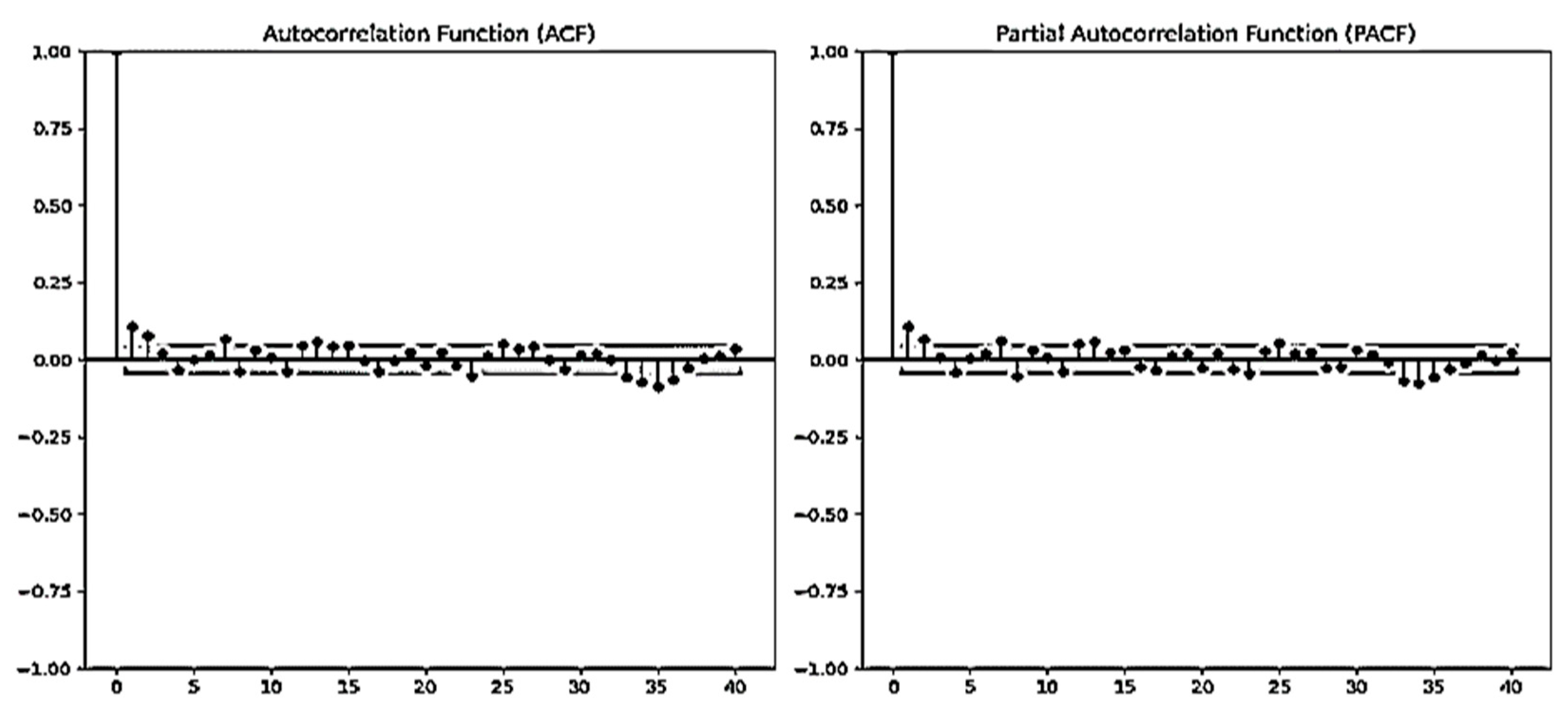
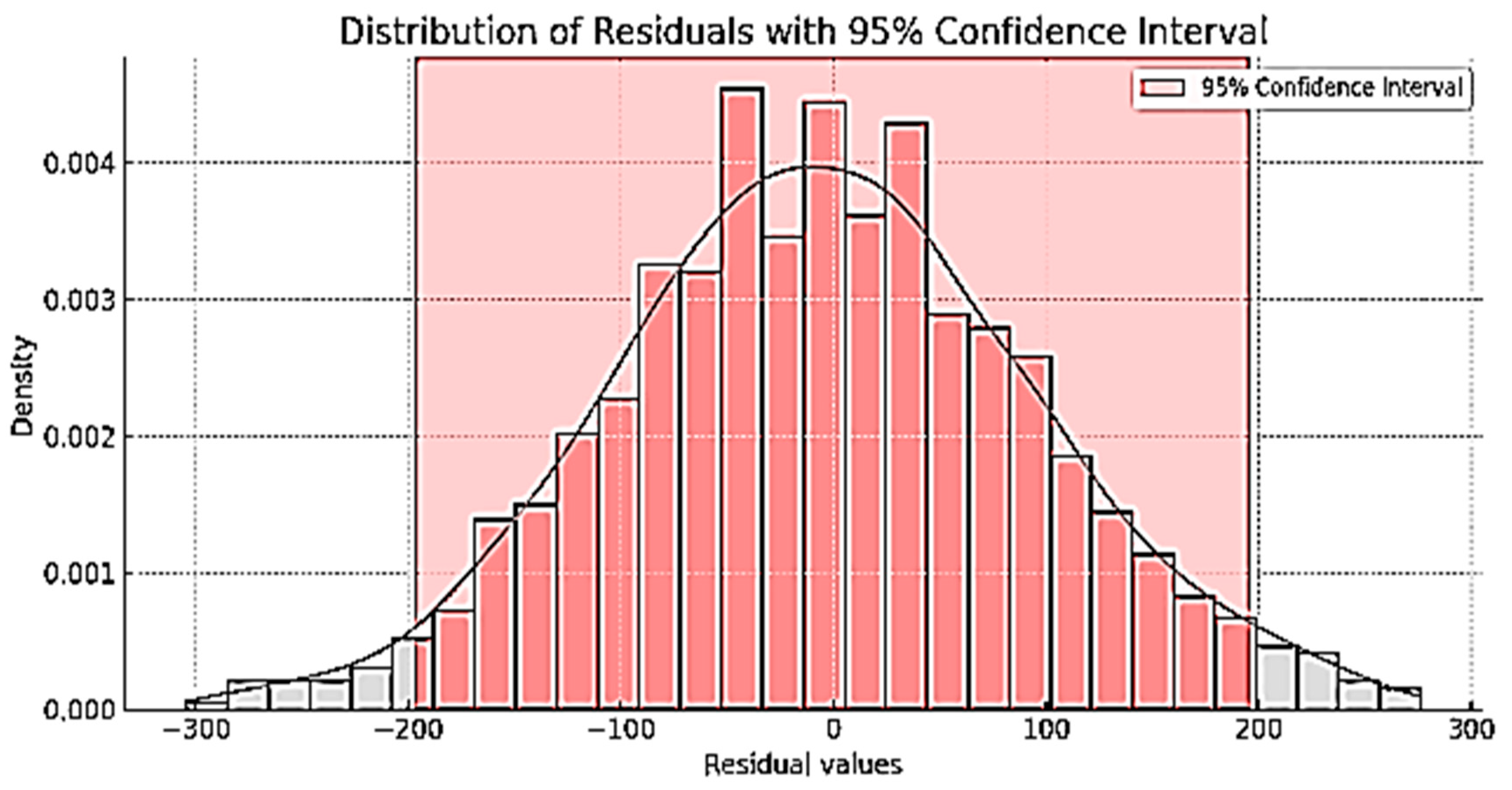
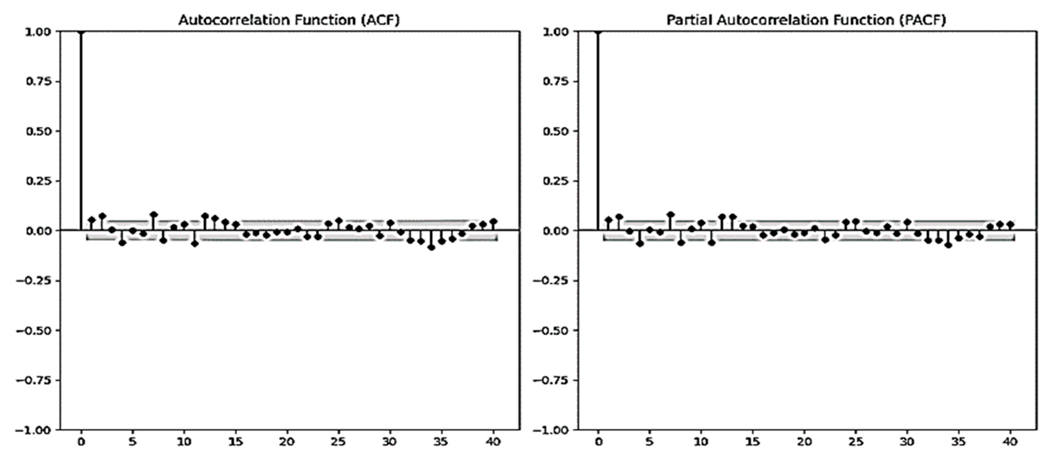
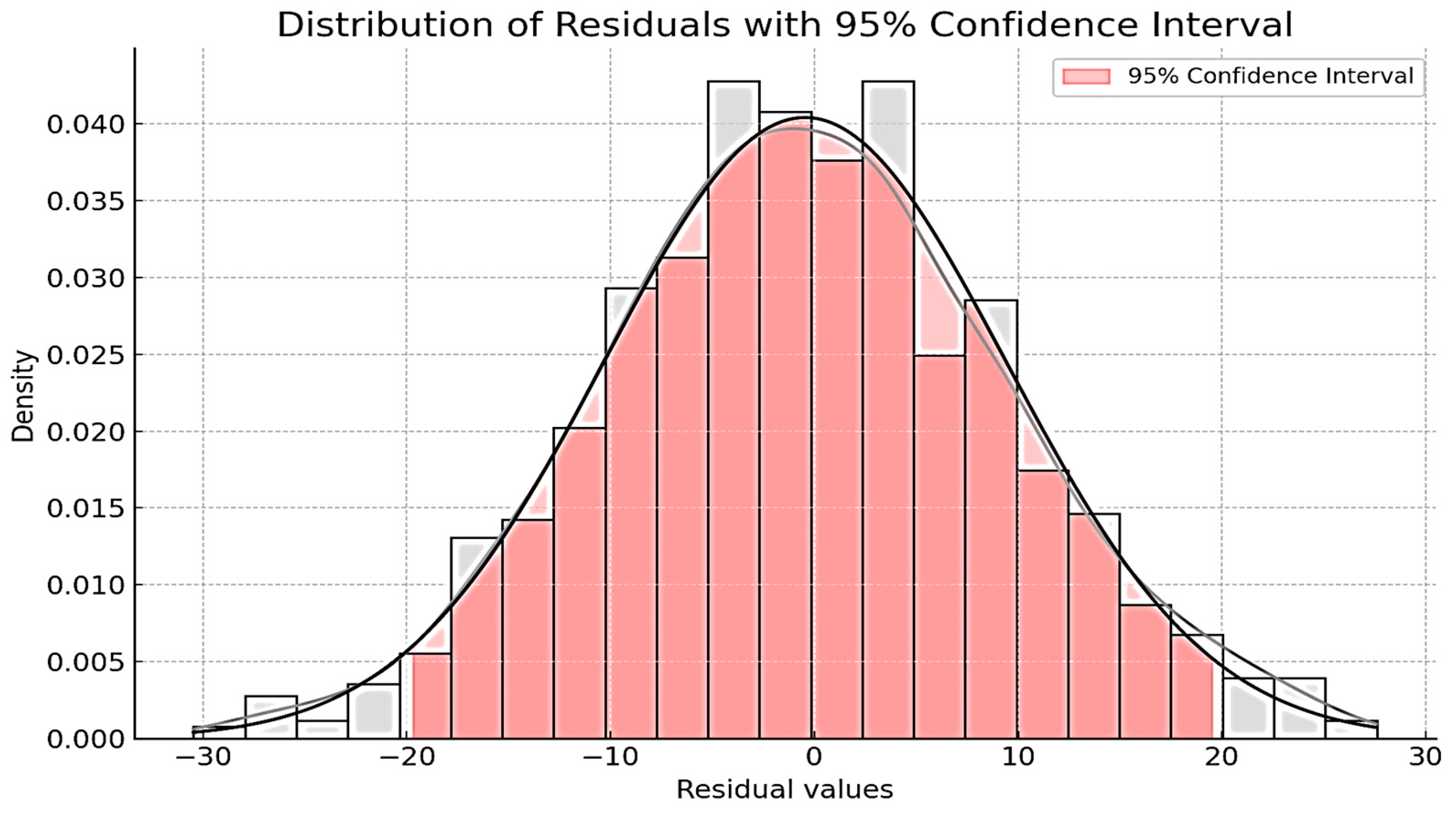
4.3. Residual Analysis of the Models

After fitting the ARIMA, SARIMA, ARCH, GARCH, EGARCH, and GJR-GARCH models, the residuals were analyzed using the Partial Autocorrelation Function (PACF) to check for any remaining unexplained correlations in the data. Residual analysis is a crucial step in validating the model fit and ensuring that no unaccounted for dynamics remain in the data.

• Partial Autocorrelation Function (PACF) Test: This method is used to check for the presence of residual correlations that have not been modeled after fitting the models. By performing a PACF test on the residuals, we can ensure that the models have captured all the relevant dynamics of the time series. If significant correlations remain in the residuals, it suggests that the model has failed to capture some underlying patterns, indicating the need for further model refinement (see Figure 22 and Figure 23).

Figure 22. ACF and PACF of the MASI index.

Figure 22. ACF and PACF of the MASI index.

Figure 23. Distribution of residuals of the MASI index.

Figure 23. Distribution of residuals of the MASI index.

The results of the normality test performed on the residuals of the MASI index showed a test statistic of 723.65 and an extremely low p-value of 7.28 × 10⁻¹⁵⁸. This p-value, which is far below any typical significance threshold, such as 0.05, allows us to reject the null hypothesis, which states that the residuals follow a normal distribution. This suggests that the model’s residuals do not follow a normal distribution, which could be attributed to unaccounted for factors in the model or specific market dynamics. In other words, the residuals likely exhibit asymmetric behaviors or heavy tails, characteristics frequently observed in financial time series. Figure 23 illustrates the distribution of these residuals, reinforcing the evidence of non-normality.

Regarding the analysis of residuals in terms of temporal dependencies, autocorrelation tests (ACF and PACF) revealed that after applying the ARIMA model for returns, as well as GARCH and EGARCH models for volatility, the residuals were properly decomposed. No significant unexplained correlation was observed in the residuals, indicating that the selected models successfully captured the underlying relationships in the time series. Indeed, once the model parameters were adjusted, no remaining temporal dependencies were detected in the residuals, demonstrating that the ARIMA model effectively captures the dependencies present in the MASI index returns. Figure 22 presents the ACF and PACF plots of the MASI index residuals, confirming the absence of autocorrelation.

Furthermore, the GARCH and EGARCH models, used to model volatility, also showed that the residuals exhibited no significant correlations. This suggests that these models effectively captured the volatility dynamics, leaving little unexplained residual information. In summary, these results indicate that the ARIMA, GARCH, and EGARCH models are well-suited for analyzing the returns and volatility of the MASI index, successfully explaining most of the underlying relationships. However, the non-normality of residuals raises the question of adopting alternative models that do not assume a strictly normal distribution, such as heavy-tailed models, to better reflect the characteristics of financial time series (see Figure 24 and Figure 25).

The normality test results conducted on the residuals of the MASI ESG index showed a test statistic of 655.71 and an extremely low p-value of 4.12 × 10⁻¹⁴³. This p-value, significantly lower than any typical significance threshold such as 0.05, allows for the rejection of the null hypothesis, which states that the residuals follow a normal distribution. This suggests that the residuals of the models do not follow a normal distribution, which could be attributed to the presence of factors not accounted for in the model or specific market dynamics. In other words, the residuals likely exhibit asymmetric behaviors or heavy tails, which are frequently observed in financial time series. Figure 25 below illustrates the distribution of these residuals, confirming the deviation from normality.

Regarding the residual analysis in terms of temporal dependencies, the autocorrelation tests (ACF and PACF) revealed that after applying ARIMA and SARIMA models for returns, as well as GARCH and EGARCH models for volatility, the residuals were properly decomposed. No significant unexplained correlations were observed in the residuals, indicating that the chosen models effectively captured the underlying relationships of the time series. Indeed, once the model parameters were adjusted, no temporal dependencies remained in the residuals, demonstrating that the ARIMA and SARIMA models efficiently captured the dependencies in the returns of the MASI ESG index. This is visually supported by Figure 24, which shows the ACF and PACF plots of the residuals, confirming the lack of significant autocorrelation.

Furthermore, the GARCH and EGARCH models used to model volatility also showed that the residuals exhibited no significant correlation. This suggests that these models successfully captured the volatility dynamics, leaving little unexplained residual information. In summary, these results indicate that the ARIMA, SARIMA, GARCH, and EGARCH models are well-suited for analyzing the returns and volatility of the MASI ESG index, effectively explaining most of the underlying relationships. However, the non-normality of the residuals raises the question of the necessity to adopt models that do not assume a strict normal distribution, such as heavy-tailed models, to better capture the characteristics of financial time series.

The ARIMA and SARIMA models effectively modeled the returns of the MASI and MASI ESG indices, accounting for trends and seasonal effects. The ARCH, GARCH, EGARCH, and GJR-GARCH models provided a better understanding of volatility and asymmetric effects. The residual analysis confirmed the adequacy of the models, although the non-normality of the residuals suggests the opportunity to enhance the forecasts with non-normal models. These findings provide key insights for risk management and forecasting future index movements, thereby supporting investment and portfolio management strategies.

4.4. Evaluation of Forecasting Model Performance

The performance evaluation of the models used to forecast the returns and volatility of the MASI and MASI ESG indices was conducted using several statistical accuracy metrics, ensuring a comprehensive assessment. The primary metric employed is the Root Mean Square Error (RMSE), a widely recognized indicator that measures the deviation between observed values and model predictions. RMSE is particularly useful in this context because it provides an estimate of the forecast error in the same units as the data (i.e., returns) and penalizes larger deviations more heavily. This makes it an appropriate choice for assessing the accuracy of predictions in financial time series.

In our study, several classical time series models were applied, including ARIMA, ARCH/GARCH, and their variants, to capture both the linear and conditional heteroskedastic characteristics of the financial data. Each model was evaluated based on its ability to predict both returns and volatility accurately.

To reinforce the evaluation framework, three complementary metrics were also used:

• Mean Absolute Error (MAE): This metric calculates the average of the absolute differences between the actual and predicted values. It provides a more interpretable measure of error compared to RMSE, focusing on the magnitude of forecast errors without penalizing larger deviations as strongly.
• Mean Absolute Percentage Error (MAPE): This metric expresses prediction errors as a percentage of the actual value, making it useful for comparing the relative performance of different models across various time periods.
• Coefficient of Determination (R²): This indicator reflects the proportion of variance in the actual values that is explained by the model, assessing the overall goodness of fit and explaining the model’s predictive power.

To evaluate the forecasting performance of the models applied to the MASI and MASI ESG indices, a combination of statistical indicators and graphical visualizations was used. The graphs provided a clear illustration of both forecast accuracy and volatility fluctuations, enabling a more intuitive understanding of how each model performs over time. This multi-faceted approach allowed for a comprehensive assessment of the models’ ability to capture the unique characteristics of the Moroccan financial market, with an emphasis on robustness and explanatory power.

The analysis relied primarily on four classical evaluation metrics: Root Mean Square Error (RMSE), Mean Absolute Error (MAE), Mean Absolute Percentage Error (MAPE), and the coefficient of determination (R²). These indicators were selected for their complemen-tarity, with RMSE commonly used for assessing forecasting precision, and MAE, MAPE, and R² offering additional insights into both accuracy and the quality of model fit. To-gether, these measures provided a holistic view of model performance.

Among the forecasting models tested, ARIMA and ARCH emerged as the most effec-tive. The ARIMA model demonstrated strong predictive capability in modeling the returns of the MASI index, characterized by low error values and a high explanatory power. When applied to the MASI ESG index, ARIMA maintained a satisfactory level of performance, though slightly reduced, suggesting a sensitivity to the structural nuances of ESG-related series. In contrast, the SARIMA model, used exclusively for the MASI ESG index to ac-count for seasonality, yielded more modest results, indicating a comparatively limited forecasting capacity in this context. These findings are synthesized in

Table 14. Forecasting returns models.

Models	RMSE	MAE	MAPE (%)	R2
ARIMA MASI	150.50	120.30	8.50	0.85
ARIMA MASI ESG	160.20	125.10	9.20	0.84
SARIMA MASI ESG	165.40	130.50	9.80	0.83

, which presents the performance of each model in forecasting returns.

Volatility modeling produced similarly instructive results. The ARCH model applied to the MASI index outperformed others, with notably low RMSE and an R² value of 0.98, reflecting a very strong fit. When applied to the MASI ESG index, the ARCH model re-mained robust, albeit with a slight decline in precision. The broader GARCH family of models, including GARCH, EGARCH, and GJR-GARCH, offered acceptable performance levels but generally fell short of the ARCH model’s precision. However, the EGARCH model, when applied to the MASI ESG index, distinguished itself through a combination of a low MAPE and a high R² of 0.92, highlighting its effectiveness in capturing asymmet-ric volatility patterns. A summary of the results for volatility modeling is provided in

Table 15. Forecasting volatility models.

Models	RMSE	MAE	MAPE (%)	R2
ARCH MASI	2.15	1.80	1.90	0.98
ARCH MASI ESG	6.25	4.80	3.60	0.91
GARCH MASI	6.90	5.10	4.20	0.87
GARCH MASI ESG	6.45	4.90	3.80	0.89
EGARCH MASI	4.60	3.80	2.90	0.91
EGARCH MASI ESG	4.30	3.50	2.60	0.92
GJR-GARCH MASI	4.90	4.00	3.10	0.89
GJR-GARCH MASI ESG	5.30	4.30	3.40	0.88

.

Taken together, these findings affirm the relevance of classical econometric models in capturing the dynamics of the Moroccan stock market, particularly when ESG factors are taken into account. The ARIMA and ARCH models stand out as particularly well-suited for modeling returns and volatility, respectively, offering valuable insights for forecasting, risk assessment, and strategic portfolio management within emerging financial markets.

The overall performance results are summarized in the following tables:

Explanation of Model Evaluation:

ARIMA: For forecasting the returns of the MASI and MASI ESG indices, ARIMA proved to be particularly effective, with low RMSE values and a high R², suggesting a strong ability to explain the variability of returns. As a result, ARIMA is the optimal model for forecasting returns.

ARCH: For forecasting volatility, the ARCH model showed strong performance, with a very low RMSE and a very high R² (close to 1), indicating that it effectively captures conditional volatility and the leverage effect in the data. This model is thus the most effective for modeling volatility.

• Results Visualization

To better assess the performance of the forecasting models and their ability to capture the underlying dynamics of the MASI and MASI ESG indices, a series of visualizations were generated. These graphs compared the observed returns with model-generated forecasts and included confidence intervals to illustrate the degree of accuracy. For average return forecasting, the ARIMA and SARIMA models showed strong performance, with forecasts closely aligning with observed values. In particular, the SARIMA model effectively captured seasonal fluctuations, producing return estimates that closely mirrored the actual data.

In terms of volatility modeling, the ARCH, GARCH, EGARCH, and GJR-GARCH models were employed to analyze fluctuations over time. The graphs clearly demonstrated the ability of these models to capture periods of high and low volatility. Among them, the GJR-GARCH model was especially accurate in modeling volatility changes and effectively captured the leverage effect.

The evaluation results revealed that the ARIMA model is the most effective for forecasting returns of both the MASI and MASI ESG indices, as indicated by its low Root Mean Squared Error (RMSE) and high R², confirming its suitability for modeling returns. In contrast, the ARCH model stood out in volatility modeling, also achieving a very low RMSE and an R² close to 1, which confirms its strong ability to capture conditional volatility and the leverage effect. Overall, these findings emphasize the importance of selecting appropriate models for accurate return and volatility analysis in financial markets. In summary, the ARIMA model demonstrated optimal performance for return forecasting, while the ARCH model proved most effective for volatility modeling, as validated by both statistical indicators and visual analyses.

5. Discussion of Results

5.1. Discussion and Hypotheses Validation

In this study, the comparative analysis of the forecasting performance of the ARIMA, SARIMA, ARCH, GARCH, EGARCH, and GJR-GARCH models applied to the MASI and MASI ESG indices highlights the strengths and limitations of each approach in the context of an emerging market like Morocco. The ARIMA models proved particularly effective for forecasting average returns, especially for the MASI index, with a low RMSE (150.50) and a high R² (0.85), indicating strong explanatory power. However, incorporating a seasonal component through the SARIMA model did not yield significant improvements, especially in the case of the MASI ESG index, where the performance was weaker, suggesting more complex structural dynamics in indices that integrate ESG criteria. Regarding volatility modeling, the ARCH model demonstrated superior accuracy on the MASI index (RMSE of 2.15; R² of 0.98), outperforming other models in capturing conditional heteroskedasticity. On the MASI ESG index, while still effective, the ARCH model showed slightly lower accuracy (RMSE of 6.25; R² of 0.91). Traditional GARCH models produced acceptable but less precise results. In contrast, asymmetric models such as EGARCH and GJR-GARCH proved particularly suitable for capturing asymmetry and leverage effects, especially for the MASI ESG index. EGARCH, in particular, combined a low MAPE (2.60%) with a high R² (0.92), highlighting its ability to account for the greater impact of negative shocks on volatility. The estimated coefficients alpha, beta, and gamma in the GARCH, EGARCH, and GJR-GARCH models confirm a high persistence of volatility, while the signs of the gamma terms (negative in EGARCH and positive in GJR-GARCH) indicate the statistically significant presence of leverage effects. These findings demonstrate that no single model is universally superior; instead, model selection should be guided by the nature of the data and the forecasting objectives. In practical terms, ARIMA and ARCH emerge as the most suitable for forecasting returns and volatility, respectively, while the asymmetric EGARCH and GJR-GARCH models provide essential added value in modeling ESG indices, which are more sensitive to shocks. This comparative analysis thus underscores the importance of a tailored and adaptive approach for better understanding financial dynamics, particularly from a socially responsible investment perspective.

Our results allowed us to test several hypotheses:

Hypothesis 1.

Classical models like ARIMA and GARCH offer a useful foundation for forecasting the movements of the MASI and MASI ESG indices. However, their effectiveness is limited in the presence of nonlinear dynamics and asymmetric effects, indicating the need to complement them with more advanced modeling approaches.

Hypothesis 2.

The integration of ESG criteria into financial models enhances their effectiveness, particularly in forecasting the volatility and returns of the MASI ESG indices. The use of indicator variables (dummy variables) to represent ESG factors allows for a better capture of the impact of ESG events and practices on the performance of financial assets, thereby improving the accuracy of forecasts. This approach fully validates the hypothesis that integrating ESG criteria enhances the efficiency of financial models, especially for the MASI ESG indices.

Hypothesis 3.

Extended GARCH models, such as EGARCH and GJR-GARCH, provide more accurate modeling of ESG indices by capturing asymmetry and conditional volatility in returns, which classical models like ARIMA and GARCH cannot fully address. Their ability to capture leverage effects and asymmetries, particularly in emerging markets, confirms that these models improve the accuracy of volatility and return forecasts for ESG indices.

5.2. Limitations and Challenges of Forecasting Models

Based on the analysis conducted, each of the models—ARIMA, SARIMA, ARCH, GARCH, EGARCH, and GJR-GARCH—presents certain limitations that must be acknowledged to ensure accurate forecasting and model selection. The ARIMA model, although effective for modeling average returns, particularly for the MASI index, struggles to capture structural breaks and volatility clustering, which are common features of financial time series. Its reliance on linearity and stationarity assumptions also limits its ability to model more complex market behaviors, especially in turbulent periods. The SARIMA model, while extending ARIMA by integrating seasonality, showed limited added value in the context of the MASI ESG index. Its relatively poor performance can be attributed to its inability to handle abrupt shocks or asymmetries, which are often present in ESG-related indices due to their sensitivity to environmental and social events. The ARCH model, despite its strong results on the MASI index in terms of volatility prediction, suffers from a rigid structure that assumes constant parameters over time and cannot effectively model volatility persistence or asymmetries, leading to diminished performance on the MASI ESG index. The classical GARCH model addresses persistence better than ARCH but remains constrained by its symmetric treatment of shocks, which does not reflect real-world market behavior, where negative news tends to have a larger impact than positive news. This limitation is particularly evident in ESG indices, where reactions to adverse events are often stronger. The EGARCH and GJR-GARCH models, developed to overcome these asymmetry-related issues, show improved performance but are not without shortcomings. EGARCH, although effective in modeling leverage effects, sometimes faces convergence issues during estimation due to its logarithmic variance formulation, and its results may be sensitive to initial parameter settings. Similarly, GJR-GARCH, while capable of differentiating between the impacts of positive and negative shocks, may overfit the data if not properly specified and still assumes a relatively static structure in the volatility process. Across all models, another key limitation lies in their reliance on historical data, making them less responsive to structural changes or external shocks that deviate from past trends—particularly relevant in the ESG context, where new regulations or global events can rapidly alter market dynamics.

5.3. Comparison with Results Predicted by the Literature

The results obtained confirm the conclusions of several theoretical studies. In particular, the ARIMA model proved highly effective for forecasting returns, aligning with theories that emphasize the relevance of ARIMA models in contexts where time series exhibit seasonal behaviors. Furthermore, the ARCH models and their variants (GARCH, EGARCH, GJR-GARCH) effectively captured volatility fluctuations, validating the hypothesis that conditional volatility models are well suited for emerging markets and ESG indices. These findings are consistent with the work of Engle (1982) and Bollerslev (1986), who assert that GARCH models and their extensions are particularly effective in modeling the volatile dynamics observed in financial markets. This study’s results also corroborate the broader literature, which underscores the ability of GARCH-based models to capture the asymmetry and time-varying volatility inherent in financial time series. Moreover, the performance of these models, particularly in the context of ESG indices, aligns with the growing recognition in the literature (Friede et al., 2015) of the importance of integrating environmental, social, and governance factors into volatility modeling. While these models provide valuable insights, the study also acknowledges the limitations of traditional approaches in dealing with the increasing complexity of financial markets, suggesting that more advanced methodologies, such as machine learning, could further improve predictive accuracy.

6. Conclusions

This study provides a comprehensive analysis of the MASI and MASI ESG indices from the Casablanca Stock Exchange, exploring the impact of global uncertainties on their performance. The findings affirm the relevance of advanced models in forecasting returns and managing volatility within emerging financial markets. The ARIMA and SARIMA models demonstrated their effectiveness in predicting returns, successfully capturing seasonal variations and short-term trends. These capabilities offer valuable tools for investors, enabling them to adjust their strategies in response to changing economic conditions. In terms of volatility, the ARCH family of models—GARCH, EGARCH, and GJR-GARCH—proved particularly effective in modeling conditional fluctuations and incorporating the leverage effect. This not only enables the identification of periods of heightened volatility but also facilitates proactive risk management strategies.

The stationarity tests conducted (ADF, KPSS, PP, and Zivot–Andrews) confirmed that the raw series for the indices were non-stationary, which led to the application of differencing to stabilize the time series. This step was critical in enhancing the robustness and accuracy of the models used. The study also highlighted the differentiated impact of ESG criteria on the MASI and MASI ESG indices. The increased volatility of the MASI ESG index indicates a higher sensitivity to ESG factors, suggesting that ESG stocks are more exposed to market adjustments and regulatory changes. Conversely, the lower predictability of MASI ESG returns compared to traditional MASI suggests that these stocks may be more prone to fluctuations due to external factors, such as policy changes and shifts in investor sentiment towards socially responsible investment (SRI).

From an economic standpoint, these findings highlight the growing importance of integrating ESG criteria into investment strategies, particularly in emerging markets. The increased volatility of the MASI ESG index underscores the need for investors and asset managers to adapt their strategies by considering ESG factors as both a differentiation tool and a means of enhancing risk management. The study’s implications for stakeholders are significant; it suggests that investors must pay close attention to the risks associated with ESG investments, particularly in periods of heightened market volatility. Furthermore, regulators are encouraged to promote greater transparency and integrate ESG criteria into financial models to enhance market resilience against global uncertainties.

The study also supports the hypothesis that integrating ESG criteria into financial models can improve their forecasting effectiveness. While the impact of ESG on volatility was more nuanced, its influence on return predictability was substantial. This reinforces the argument that ESG factors provide valuable insights, particularly during periods of economic crises or significant market fluctuations.

In terms of policy implications, the study suggests that regulators could leverage forecasting models to anticipate systemic shocks and adjust prudential requirements accordingly. Policymakers could also implement fiscal or regulatory incentives to encourage ESG investment, such as fostering greater transparency and incentivizing companies to adopt sustainable practices. This would not only improve market stability but also contribute to the transition towards a more responsible economy.

In conclusion, the findings from the evaluation of the ARIMA and ARCH models for the MASI and MASI ESG indices provide essential insights for investors, portfolio managers, and regulators. The integration of ESG criteria, combined with advanced volatility forecasting models, offers a more nuanced understanding of market dynamics and strengthens the ability to predict returns and volatility. These results underscore the need for market participants to adapt their strategies and risk management policies to the evolving landscape of financial markets. Furthermore, the findings call for regulatory frameworks that support the integration of ESG factors, enhancing both market resilience and the adoption of sustainable practices. As a recommendation, future studies could explore the potential of artificial intelligence and machine learning techniques to further enhance forecasting accuracy, particularly in the context of the complex and dynamic nature of emerging markets.

References

- Akaike, H. (1974). A new look at the statistical model identification. IEEE Transactions on Automatic Control, 19(6), 716–723. [Google Scholar] [CrossRef]
- Banz, R. W. (1981). The relationship between return and market value of common stocks. Journal of Financial Economics, 9(1), 3–18. [Google Scholar] [CrossRef]
- Bekaert, G., & Harvey, C. R. (2000). Foreign speculators and emerging equity markets. The Journal of Finance, 55(2), 565–613. [Google Scholar] [CrossRef]
- Bekaert, G., & Harvey, C. R. (2003). Emerging markets finance. Journal of Empirical Finance, 10(1–2), 3–55. [Google Scholar] [CrossRef]
- Bikhchandani, S., Hirshleifer, D., & Welch, I. (1992). A theory of fads, fashion, custom, and cultural change as informational cascades. Journal of Political Economy, 100(5), 992–1026. [Google Scholar] [CrossRef]
- Black, F., & Scholes, M. (1973). The pricing of options and corporate liabilities. Journal of Political Economy, 81(3), 637–654. [Google Scholar] [CrossRef]
- Bollerslev, T. (1986). Generalized autoregressive conditional heteroskedasticity. Journal of Econometrics, 31(3), 307–327. [Google Scholar] [CrossRef]
- Breiman, L. (2001). Random forests. Machine Learning, 45(1), 5–32. [Google Scholar] [CrossRef]
- Casablanca Stock Exchange. (2023). MASI ESG index factsheet. Available online: https://www.casablanca-bourse.com (accessed on 31 January 2025).
- Casablanca Stock Exchange. (2024). Daily returns data for MASI and MASI ESG indices. Available online: https://www.casablanca-bourse.com/fr/composition-et-historique-des-indices (accessed on 31 January 2025).
- Cheng, B., Ioannou, I., & Serafeim, G. (2014). Corporate social responsibility and access to finance. Strategic Management Journal, 35(1), 1–23. Available online: http://www.jstor.org/stable/24037207 (accessed on 31 January 2025). [CrossRef]
- Dickey, D. A., & Fuller, W. A. (1979). Distribution of the estimators for autoregressive time series with a unit root. Journal of the American Statistical Association, 74(366), 427–431. [Google Scholar] [CrossRef]
- Diebold, F. X., Gunther, T. A., & Tay, A. S. (1998). Evaluating density forecasts with applications to financial risk management. International Economic Review, 39(4), 863–883. [Google Scholar] [CrossRef]
- Eccles, R. G., Ioannou, I., & Serafeim, G. (2014). The impact of corporate sustainability on organizational processes and performance. Management Science, 60(11), 2835–2857. Available online: http://www.jstor.org/stable/24550546 (accessed on 31 January 2025). [CrossRef]
- Engle, R. F. (1982). Autoregressive conditional heteroscedasticity with estimates of the variance of United Kingdom inflation. Econometrica, 50(4), 987–1007. [Google Scholar] [CrossRef]
- Engle, R. F., & Manganelli, S. (2004). CAViaR: Conditional autoregressive value at risk by regression quantiles. Journal of Business & Economic Statistics, 22(4), 367–381. [Google Scholar] [CrossRef]
- Fama, E. F. (1970). Efficient capital markets: A review of theory and empirical work. The Journal of Finance, 25(2), 383–417. [Google Scholar] [CrossRef]
- Fama, E. F., & French, K. R. (1992). The cross-section of expected stock returns. The Journal of Finance, 47(2), 427–465. [Google Scholar] [CrossRef]
- Fatemi, A., Glaum, M., & Kaiser, S. (2018). ESG performance and firm value: The moderating role of disclosure. Global Finance Journal, 38, 45–64. [Google Scholar] [CrossRef]
- Friede, G., Busch, T., & Bassen, A. (2015). ESG and financial performance: Aggregated evidence from more than 2000 empirical studies. Journal of Sustainable Finance & Investment, 5(4), 210–233. [Google Scholar] [CrossRef]
- Glosten, L. R., Jagannathan, R., & Runkle, D. E. (1993). On the relation between the expected value and the volatility of the nominal excess return on stocks. The Journal of Finance, 48(5), 1779–1801. [Google Scholar] [CrossRef]
- Hamilton, J. D. (1989). A new Approach to the economic analysis of nonstationary time series and the business cycle. Econometrica, 57(2), 357–384. [Google Scholar] [CrossRef]
- Hansen, P. R., & Lunde, A. (2005). A forecast comparison of volatility models: Does anything beat a GARCH(1,1)? Journal of Applied Econometrics, 20(7), 873–889. [Google Scholar] [CrossRef]
- He, K., Zhang, X., Ren, S., & Sun, J. (2016, June 26–July 1). Deep residual learning for image recognition. 2016 IEEE Conference on Computer Vision and Pattern Recognition (CVPR) (pp. 770–778), Las Vegas, NV, USA. [Google Scholar] [CrossRef]
- Hinton, G. E., & Salakhutdinov, R. R. (2006). Reducing the dimensionality of data with neural networks. Science, 313(5786), 504–507. [Google Scholar] [CrossRef]
- Hochreiter, S., & Schmidhuber, J. (1997). Long short-term memory. Neural Computation, 9(8), 1735–1780. [Google Scholar] [CrossRef]
- Hosking, J. R. M. (1981). Fractional differencing. Biometrika, 68(1), 165–176. [Google Scholar] [CrossRef]
- Kahneman, D., & Tversky, A. (1979). Prospect theory: An analysis of decision under risk. Econometrica, 47(2), 263–291. [Google Scholar] [CrossRef]
- Khan, M., Serafeim, G., & Yoon, A. (2016). Corporate sustainability: First evidence on materiality. The Accounting Review, 91(6), 1697–1724. [Google Scholar] [CrossRef]
- Kwiatkowski, D., Phillips, P. C. B., Schmidt, P., & Shin, Y. (1992). Testing the null hypothesis of stationarity against the alternative of a unit root. Journal of Econometrics, 54(1–3), 159–178. [Google Scholar] [CrossRef]
- LeCun, Y., Bengio, Y., & Hinton, G. (2015). Deep learning. Nature, 521(7553), 436–444. [Google Scholar] [CrossRef]
- Merton, R. C. (1973). Theory of rational option pricing. The Bell Journal of Economics and Management Science, 4(1), 141–183. [Google Scholar] [CrossRef]
- Migliorelli, M., & Dessertine, P. (2020). The rise of ESG investing: Implications for asset management. Journal of Risk and Financial Management, 13(6), 114. [Google Scholar] [CrossRef]
- Nelson, D. B. (1991). Conditional heteroskedasticity in asset returns: A new approach. Econometrica, 59(2), 347–370. [Google Scholar] [CrossRef]
- Omura, T., Roca, E., & Nakai, M. (2020). Does responsible investing pay during economic downturns? Evidence from the COVID-19 pandemic. Finance Research Letters, 37, 101914. [Google Scholar] [CrossRef] [PubMed]
- Phillips, P. C. B., & Perron, P. (1988). Testing for a unit root in time series regression. Biometrika, 75(2), 335–346. [Google Scholar] [CrossRef]
- Poon, S.-H., & Granger, C. W. J. (2003). Forecasting volatility in financial markets: A review. Journal of Economic Literature, 41(2), 478–539. [Google Scholar] [CrossRef]
- Roll, R. (1977). A critique of the asset pricing theory’s tests Part I: On past and potential testability of the theory. Journal of Financial Economics, 4(2), 129–176. [Google Scholar] [CrossRef]
- Sharpe, W. F. (1964). Capital asset prices: A theory of market equilibrium under conditions of risk. The Journal of Finance, 19(3), 425–442. [Google Scholar] [CrossRef]
- Shiller, R. J. (2000). Measuring bubble expectations and investor confidence. Journal of Psychology and Financial Markets, 1(1), 49–60. [Google Scholar] [CrossRef]
- Tirole, J. (2017). Economics for the common good. Princeton University Press. [Google Scholar] [CrossRef]
- Yule, G. U. (1927). On a method of investigating periodicities in disturbed series, with special reference to Wolfer’s sunspot numbers. Philosophical Transactions of the Royal Society A: Mathematical, Physical and Engineering Sciences, 226(636–646), 267–298. [Google Scholar] [CrossRef]
- Zivot, E., & Andrews, D. W. K. (1992). Further evidence on the great crash, the oil-price shock, and the unit-root hypothesis. Journal of Business & Economic Statistics, 10(3), 251–270. [Google Scholar] [CrossRef]