From Disruption to Integration: Cryptocurrency Prices, Financial Fluctuations, and Macroeconomy

Abstract

This paper examines cryptocurrency shock transmission to financial markets and the macroeconomy using a Bayesian structural VAR with Pandemic Priors from 2015 to 2024. By affecting overall risk appetite, cryptocurrency price shocks generate positive financial market spillovers, accounting for 18% of equity and 27% of commodity price fluctuations. Real economic effects are significant in driving investment but remain limited, contributing only 4% to unemployment and 6% to industrial production variance. However, cryptocurrency shocks explain 18% of price-level forecast error variance at long horizons. Narrative analysis reveals sentiment and technology as primary shock drivers. These findings demonstrate cryptocurrency’s deep financial system integration with important inflation implications for monetary policy.

1. Introduction

Cryptocurrency has evolved from negligible value to a major multi-trillion-dollar asset class, reaching an all-time high of USD 3.8 trillion in January 2025. Bitcoin alone surged from under USD 0.001 in 2010 to over USD 111,000 in May 2025 with extraordinary volatility and growth over more than a decade. Institutional adoption has accelerated integration with the existing finance markets: MicroStrategy holds 582,000 bitcoins worth approximately USD 61.25 billion, making it the world’s largest corporate bitcoin holder. Bitcoin ETFs have achieved remarkable success, with 12 spot Bitcoin ETFs collectively surpassing USD 100 billion in assets under management and holding over 1.1 million bitcoin (about 5% of all bitcoin in existence). This rapid evolution from speculative experiment to mainstream financial asset raises critical questions about cryptocurrency’s transmission effects on financial systems and the broader economy.

Understanding these dynamics requires identifying what drives such price changes. Cryptocurrencies respond to shocks across various areas: technological developments (protocol upgrades, network improvements), regulatory changes (legal recognition, trading restrictions), monetary policy shifts affecting demand for alternative assets, infrastructure developments (exchange launches, institutional adoption), network effects (user growth, corporate integration), and sentiment-driven events that reflect market psychology and speculation. The different nature of these driving forces raises important questions. Do policies primarily influence cryptocurrency markets, making them vulnerable to regulatory and monetary oversight? Do technological advances and network growth drive persistent price changes? Do sentiment and speculation dominate, disconnecting bitcoin markets from economic fundamentals?

In addition to being a source of price innovations, cryptocurrency spillovers to the financial system and real economic activity represent another important dimension to explore. Do traditional financial connections through bank loans and household wealth fully capture how crypto assets transmit their effects? The decentralized nature of cryptocurrency markets, their global accessibility, and their integration with emerging financial technologies create new pathways through which digital asset movements influence economic outcomes. Recent institutional adoption by businesses, pension funds, and sovereign wealth funds has created direct balance sheet exposures, while cryptocurrency-backed lending and derivatives have deepened integration with the finance system. Then what is the macroeconomic implication of such financial integration?

This paper attempts to fill three critical gaps that remain unaddressed in this rapidly growing literature. First, no study has systematically validated cryptocurrency shock identification through narrative analysis across multiple event categories. Second, existing studies predominantly employ correlation-based measures that cannot establish causality between cryptocurrency movements and macroeconomic outcomes. Third, it lacks methodology in structural modeling, which is capable of handling extreme crisis periods like COVID-19 when conventional econometric relationships deteriorate.

To address these questions, this paper examines bitcoin price shock transmission using a Bayesian structural vector autoregression (BSVAR) framework that incorporates Pandemic Priors to handle extreme observations during COVID-19. This approach isolates the cryptocurrency shocks that are independent of simultaneous movements in macroeconomic and financial variables, then traces how these shocks affect inflation, unemployment, industrial production, monetary aggregates, equity prices, commodities, and financial stress indicators.

This study validates the identified cryptocurrency shocks through narrative analysis, systematically categorizing bitcoin events into six types: technological, sentiment, monetary, regulatory, infrastructure, and network effect shocks. This method provides external validation and reveals which event types consistently drive cryptocurrency market innovations. Variance decomposition is further utilized to measure how much cryptocurrency shocks contribute to fluctuations in macroeconomic and financial variables over different time periods.

This study reveals three key insights. First, it finds spillover effects on financial markets via shifting overall risk appetite and driving comovement across financial asset categories. Second, it evaluates transmission mechanisms to the economy, which is significantly expansionary yet limited in magnitude. Third, sentiment and technology drive exogenous crypto innovations.

The empirical findings carry implications for monetary authorities and financial regulators, suggesting the need for systematic monitoring of cryptocurrency spillovers and incorporation of these developments into policy frameworks.

2. Literature Review

The cryptocurrency literature has rapidly evolved to examine both the drivers of crypto market dynamics and their spillover to broader financial and economic systems. This synthesis reviews research across three interconnected areas: identifying cryptocurrency shock sources, analyzing the spillover to financial markets, and exploring the largely uncharted territory of macroeconomic transmission channels.

2.1. Sources and Identification of Cryptocurrency Shocks

As cryptocurrency markets have expanded in both size and influence, understanding the origins of price movements has gained critical importance. While the literature recognizes multiple sources of exogenous innovations, systematic classification remains underdeveloped. Technology shocks—such as protocol upgrades, hard forks, and network improvements—constitute fundamental drivers that set cryptocurrencies apart from other mainstream financial assets (Brandvold et al., 2015; Liu et al., 2021).

Regulatory developments emerge as another pivotal source of cryptocurrency price innovations. Empirical evidence reveals asymmetric responses to policy announcements and enforcement actions (Auer & Claessens, 2018; Chokor & Alfieri, 2021). The global nature of cryptocurrency markets amplifies regulatory impact, as demonstrated by Borri and Shakhnov (2020), who show that policy changes in major jurisdictions transmit worldwide due to the borderless characteristics of digital asset trading. In contrast to regulatory shocks, sentiment-driven innovations stem from institutional adoption announcements, media coverage, and collective investor psychology and they exhibit notable persistence while creating distinct volatility clustering patterns (Demir et al., 2018; Wu et al., 2019).

Rather than operating through direct liquidity channels, monetary policy influences on cryptocurrency markets primarily function via portfolio rebalancing mechanisms (Bouri et al., 2017). Meanwhile, network effect shocks arising from adoption milestones, corporate integration, and ecosystem developments generate positive feedback loops that cascade across interconnected cryptocurrency platforms.

Although the list of determinants of cryptocurrency returns continues expanding, most studies concentrate on individual shock categories or rely on correlation-based methodologies that fail to establish causality. This research advances beyond these limitations by systematically categorizing events into six shock types while employing narrative regression analysis for structural identification validation. This approach represents the first rigorous application of narrative identification techniques to cryptocurrency markets, drawing on proven success in monetary policy literature (Romer & Romer, 2004).

2.2. Financial Market Transmission Mechanisms

The propagation of cryptocurrency shock to other financial markets operates fundamentally through mechanisms established by modern portfolio theory. Seminal work from Markowitz (1952) demonstrated that rational investors construct portfolios based on expected returns, variances, and covariances, creating the theoretical foundation for understanding how shocks to one asset class propagate through portfolio rebalancing to affect other assets. This framework was extended by Tobin (1958) and Tobin (1969), whose Portfolio Balance Theory explains how investors adjust their asset holdings in response to price changes to maintain optimal risk-return profiles.

Portfolio theory generates specific predictions about how cryptocurrency price movements affect financial assets. When cryptocurrency prices increase, portfolio rebalancing mechanisms create spillover effects to other assets, depending on their correlation structure and portfolio weights. The Capital Asset Pricing Model from Sharpe (1964) predicts that assets with similar systematic risk exposures should exhibit stronger comovement patterns, explaining why cryptocurrency shocks primarily affect equity markets while notably excluding bonds or commodities (Caporale et al., 2018; Katsiampa et al., 2019). The selective nature of these spillovers reflects the risk characteristics of cryptocurrencies as speculative growth assets rather than safe havens or inflation hedges.

Beyond portfolio effects, behavioral finance theory explains how cryptocurrency price movements signal broader shifts in risk appetite. Work by Baker and Wurgler (2007) on an investor sentiment framework demonstrates how mood-driven trading creates systematic factors affecting all risky assets, while work by Christie and Huang (1995) on herding behavior predicts that retail-dominated markets like cryptocurrencies serve as leading indicators of broader risk appetite. Crisis periods amplify these dynamics through Forbes and Rigobon (2002) contagion mechanisms, where diversification benefits vanish and cryptocurrencies display elevated correlations with other speculative assets during market stress (Charfeddine et al., 2020).

Institutional participation further alters how cryptocurrency prices affect other financial markets by creating direct financial linkages. Work by Brunnermeier and Pedersen (2009) on funding liquidity theory explains how institutional leverage and margin requirements create transmission channels between asset markets, suggesting enhanced institutional involvement may transform cryptocurrencies from isolated speculative assets to integrated components of the global financial system. These developments strengthen the transmission of cryptocurrency price shocks to other financial markets through institutional portfolios, derivative markets, and cross-border arbitrage strategies.

2.3. Macroeconomic Transmission: An Understudied Area

Despite extensive documentation of financial market spillovers, macroeconomic transmission mechanisms of cryptocurrency price shocks remain understudied. This line of research can be traced back to Keynes (1937) aggregate demand framework and Hicks (1937) IS-LM model, arguing that asset price changes should transmit to real economic activity when asset markets reach sufficient size and integration.

From the household perspective, the wealth effect channel, formalized by Modigliani and Brumberg (1954) life-cycle hypothesis and extended by Ando and Modigliani (1963), predicts that cryptocurrency appreciation increases household net worth, leading to higher consumption and aggregate demand. Case et al. (2005) demonstrate that wealth effects operate most strongly for assets perceived as permanent stores of value, suggesting that cryptocurrency’s evolution from speculative instrument to institutional asset class should strengthen this transmission mechanism.

From the supply side, the investment channel operates through Tobin (1969) Q theory, where cryptocurrency price movements may influence venture capital flows and technology sector investment through the relative cost of new capital formation. Jermann and Quadrini (2012) demonstrate that asset price volatility creates real options effects on investment timing, while Bloom (2009) show that uncertainty shocks delay irreversible investment decisions. Those investment-related channels predict the real effects of cryptocurrency shocks.

Financial markets amplify these direct transmission mechanisms through credit and balance sheet channels, as identified by Bernanke et al. (1999)’s financial accelerator model. This framework predicts that financial asset price changes affect balance sheets of firms and financial intermediaries, which in turn influence the credit availability and credit spreads. Adrian and Shin (2010) demonstrate that asset price volatility affects financial intermediary capacity, while He and Krishnamurthy (2013) show how dealer constraints create procyclical leverage effects.

Despite these strong theoretical foundations, existing empirical research exhibits critical limitations, such as unidirectional focus on financial spillovers while neglecting macroeconomic transmission, inadequate handling of structural breaks during crisis periods, and a lack of comprehensive feedback effect analysis.

To address these gaps, this study employs a structural VAR model incorporating cryptocurrency returns, financial variables (stocks, bonds, exchange rates), and macroeconomic indicators (industrial production, prices, unemployment, monetary aggregates). Cascaldi-Garcia (2022) Pandemic Priors is implemented to preserve structural relationships during COVID-19 disruption. This analysis directly examines the transmission mechanisms and feedback loops that theory predicts but the literature inadequately examines.

3. Data and Methods

A monthly Bayesian VAR in levels with the following eight endogenous variables is estimated.

Three macroeconomic variables are included. The (log) PCE price index serves as the measure of inflation, capturing the price level of personal consumption expenditures. The CPI is considered as a robustness check. Industrial production in log levels represents real economic activity and has historically displayed extreme variations during economic downturns. The unemployment rate provides a direct measure of labor market conditions, representing the number of unemployed as a percentage of the labor force.

The monetary variable is the (log) Barnett (1980) Divisia M4 index obtained from the Center of Financial Stability. It provides a more accurate and broader measure of money supply than conventional simple-sum approaches (Chen & Valcarcel, 2025a). While conventional measures simply add up different types of monetary assets equally—like regarding cash, savings accounts, and term deposits as equivalent—Divisia M4 recognizes that not all monetary assets are created equal. It assigns different weights to monetary components based on how easily they can be spent, giving more importance to highly liquid forms like cash and checking accounts, and less weight to money tied up in certificates of deposit or other less liquid forms. The monetary aggregates using the Divisia method become particularly valuable for indicating monetary policy when short-term interest rates approach zero and become uninformative (Chen & Valcarcel, 2021, 2025b; Keating et al., 2019).

The SVAR includes four financial variables, including the bitcoin price. The (log) S&P 500 index represents equity market valuations. The Commodity Research Bureau (CRB) commodity index is a representative indicator of global commodity markets and measures the aggregated price direction of various commodity sectors. It serves as an ad hoc solution in Christiano et al. (1999) to resolve the price puzzle and is then widely used to incorporate forward-looking information in an SVAR system. We include the (log) cryptocurrency price level, indicated by bitcoin price, as a measure of alternative asset pricing and digital financial innovation. Lastly, the baseline model incorporates the financial stress index generated by the St. Louis Fed, which captures financial market conditions and overall financial stress. The excess bond premium (EBP) constructed by Gilchrist and Zakrajšek (2012) and the Cleveland financial stress index are considered as alternatives.

The sample period extends from January 2015 through November 2024. The sample begins in January 2015 rather than Bitcoin’s 2010 inception for three reasons: (1) Bitcoin price data before 2015 exhibits extreme volatility and thin trading that could distort VAR estimates; (2) the focus on macroeconomic transmission requires Bitcoin to have achieved sufficient market capitalization to plausibly affect broader markets; (3) Bitcoin’s market structure fundamentally changed around 2014–2015 with the emergence of regulated exchanges, institutional infrastructure, and standardized trading protocols, making pre-2015 data less representative of cryptocurrency markets integrated with the financial system.

Importantly, this sample period spans the COVID-19 pandemic, necessitating the use of Pandemic Priors to properly account for the extreme observations during this period.

3.1. Pandemic Prior

The onset of the COVID-19 pandemic caused macroeconomic variables to display complex patterns that hardly follow any historical pattern. From an empirical perspective, this episode poses a challenge to how to deal with such unusual behavior while retaining historical relationships, producing reliable forecasts, and providing correct interpretations of economic shocks.

Employing conventional Minnesota priors could be misleading, as a very low number of extreme pandemic observations distort the estimated persistence of the variables, affecting forecasts and giving a myopic view of the economic effects after a structural shock. Instead, a straightforward solution is adopted to deal with these extreme episodes by extending the Minnesota Prior with time dummies (Cascaldi-Garcia, 2022). The technical details are provided in Appendix B; this subsection outlines the key features of the estimation methodology.

Following the notation from Bańbura et al. (2010), the baseline model takes a VAR setup with n variables, T periods, and p lagsas

$${\mathbf{Y}}_t=\mathbf{c}+{\mathbf{1}}_{t=a+1}{\mathbf{d}}_{a+1}+\dots +{\mathbf{1}}_{t=a+h}{\mathbf{d}}_{a+h}+{\mathbf{A}}_1{\mathbf{Y}}_{t-1}+\dots +{\mathbf{A}}_p{\mathbf{Y}}_{t-p}+{\mathbf{u}}_t$$

(1)

where ${\mathbf{d}}_{a+1}$ through ${\mathbf{d}}_{a+h}$ are h vectors with n time dummies for a predefined number of h periods from $t=a+1$ through $t=a+h$ (which can be the COVID-19 crisis), and ${\mathbf{1}}_{t=i}$ is an indicator function that takes the value 1 for the pandemic periods and 0 otherwise. This structure extends the VAR to the idea that there may be an abnormal period when the relationship between the variables diverges from history.

The parameter $\varphi$ plays an important role for the Pandemic Priors, as it governs the prior associated with the time dummies. When $\varphi \to 0$, the prior for the time dummies is fairly uninformative, and the time dummies soak the variance of the pandemic period—essentially treating these observations as extraordinary events that should not influence our understanding of normal economic relationships. When $\varphi \to \infty$, full signal is taken from the pandemic period, the time dummies shrink toward zero, and that information is treated as any other observation—forcing the model to explain extreme pandemic variations through standard economic coefficients, potentially distorting them. The Pandemic Priors nest the boundary cases of an uninformative prior that soaks all the variance and a conventional Minnesota Prior, with the optimal $\varphi$ striking a balance between acknowledging the unusual nature of pandemic data while still extracting useful information from it.

A data-driven method is adopted to select the optimal level of $\varphi$ by finding the one that maximizes the marginal density of the model, defined as ${\varphi }^{\ast }=arg{max}_{\varphi }ln{p}_{\varphi }\left(\mathbf{Y}\right)$. If the optimal ${\varphi }^{\ast }\to \infty$, the data favor a model with a conventional Minnesota Prior. If the optimal ${\varphi }^{\ast }\to 0$, the data favor a model in which the observations from the selected period are downplayed to some degree, and the time dummies from the Pandemic Priors become active.

The overall prior tightness is set as $\lambda =0.2$ and $\varphi$ is optimally selected at ${\varphi }^{\ast }=0.1$ in the baseline model. This low value suggests the necessity of using the Pandemic Prior approach, as it indicates that the data strongly favor a model in which the observations from the pandemic period are substantially downplayed, and thus the time dummies from the Pandemic Priors become active in capturing the unusual relationships during this extreme episode.

3.2. Identification Strategy and Analysis

The structural identification in the structural VAR employs recursive ordering. The complete recursive ordering is as follows: (1) PCE price index; (2) unemployment rate; (3) industrial production; (4) Divisia M4; (5) cryptocurrency price; (6) S&P 500; (7) CRB commodity index; (8) Financial Stress Index.

The mapping between reduced-form residuals and structural shocks is given by the following:

$${\mathbf{u}}_t={\mathbf{A}}_0^{-1}{\epsilon }_t$$

where ${\mathbf{u}}_t$ is the vector of reduced-form residuals, ${\epsilon }_t$ is the vector of structural shocks, and ${\mathbf{A}}_0$ is the contemporaneous coefficient matrix. Under recursive identification, ${\mathbf{A}}_0$ is lower triangular:

$${\mathbf{A}}_0=\left(\begin{array}{cccccccc}1& 0& 0& 0& 0& 0& 0& 0\\ a_{21}& 1& 0& 0& 0& 0& 0& 0\\ a_{31}& a_{32}& 1& 0& 0& 0& 0& 0\\ a_{41}& a_{42}& a_{43}& 1& 0& 0& 0& 0\\ a_{51}& a_{52}& a_{53}& a_{54}& 1& 0& 0& 0\\ a_{61}& a_{62}& a_{63}& a_{64}& a_{65}& 1& 0& 0\\ a_{71}& a_{72}& a_{73}& a_{74}& a_{75}& a_{76}& 1& 0\\ a_{81}& a_{82}& a_{83}& a_{84}& a_{85}& a_{86}& a_{87}& 1\end{array}\right)$$

This ordering follows standard macroeconomic VAR literature (e.g., Christiano et al. (1999); Ramey (2016)) where slow-moving variables (prices, output, employment) precede fast-moving financial variables. Cryptocurrency is ordered fifth to allow contemporaneous responses to macroeconomic fundamentals while restricting contemporaneous feedback to financial variables. Importantly, the main findings are robust to alternative variable orderings, as demonstrated in the robustness checks (Section 6.1). Specifically, a test of positioning cryptocurrency price, which is the last within the recursive structure, shows virtually indistinguishable impulse response functions.

After estimating the reduced-form VAR parameters and the mapping matrix, the impulse response functions are generated to trace cryptocurrency shock transmission mechanisms to both financial and macroeconomic variables over 30-month horizons. These impulse responses reveal the dynamic path of adjustment in those included variables following a one-standard-deviation positive cryptocurrency shock. The confidence bands are calculated using posterior draws from the Bayesian estimation.

Forecast error variance decompositions at 6, 12, and 30 months quantify the relative importance of crypto shocks in explaining fluctuations across different time horizons. These decompositions reveal what percentage of the forecast error variance in each variable can be attributed to cryptocurrency innovations at short, medium, and long-term horizons.

To validate the identification strategy and provide an economic interpretation of the estimated shock series, a narrative approach is implemented, examining the correspondence between the estimated structural shocks and historical cryptocurrency events. A detailed list of cryptocurrency market developments in the sample is constructed.

For each event category, dummy variables are constructed and narrative regressions are estimated where the estimated structural cryptocurrency shock series serves as the dependent variable. The explanatory variables include dummy variables for each event category in each month. The coefficient on each event category dummy variable measures the average magnitude of crypto shocks associated with that particular type of event. This approach tests whether the identified shocks systematically correspond to observable cryptocurrency market events and, in turn, validates that the structural identification captures meaningful economic developments in the cryptocurrency space rather than statistical artifacts. The robustness analysis includes sensitivity checks across multiple dimensions. Alternative variable orderings in the SVAR are examined, testing different positions for cryptocurrency in the recursive identification scheme.

Alternative measures for key variables are substituted, including CPI inflation instead of PCE, the excess bond premium, and the Cleveland financial stress index instead of the St. Louis measure. The Pandemic Prior specifications are further varied, testing different values of $\varphi$ and alternative pandemic period definitions.

4. Results

4.1. Impulse Responses to Crypto Shocks

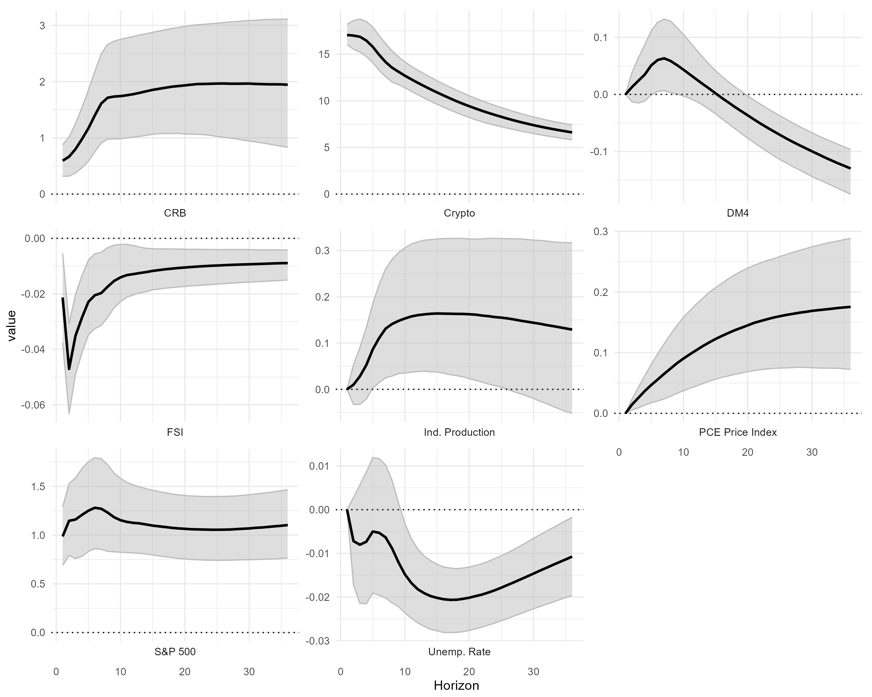
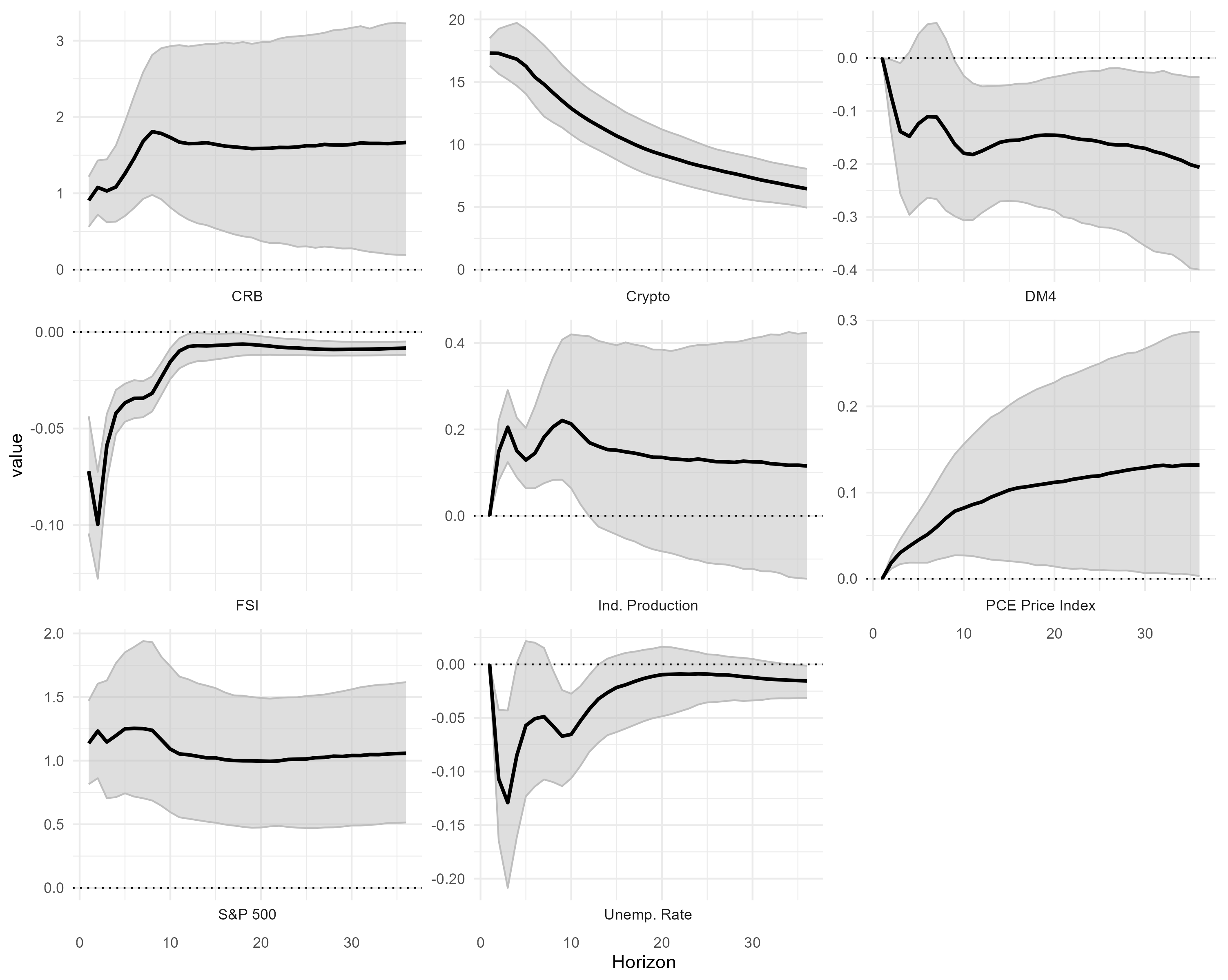
Figure 1 shows impulse responses that are generated from the Bayesian VAR model using the Pandemic Prior. The responses are the dynamic effects of a one-standard-deviation positive cryptocurrency shock (demonstrated by a 15.8% exogenous increase of the bitcoin price) on all eight endogenous variables over a 30-month horizon. The black solid lines represent the median responses, while the gray shaded areas indicate the credible intervals (68% posterior probability bands).

The sustained 1.2% increase of the S&P 500 index and the CRB commodity response of 2% provide direct empirical validation of modern portfolio theory, i.e., assets with similar systematic risk exposures exhibit stronger comovement patterns, and cryptocurrencies show integration to risk assets rather than isolated speculative instruments. The Financial Stress Index’s initial drastic alleviation, followed by recovery, further suggests that the overall risk appetite varies with crypto shocks.

The delayed 0.15% positive response of industrial production and the persistent 0.02% decline in unemployment validate investment-related channels where asset price movements influence investment through relative capital costs, with timing reflecting real options effects, where firms optimize irreversible decisions based on market conditions. Unemployment drop may also operate through life-cycle wealth effects, where cryptocurrency appreciation increases household net worth, leading to higher consumption and aggregate demand. Furthermore, it is premature to rule out the role of a financial accelerator, with which the improvement in the credit condition, signaled by the alleviated financial stress, enhances economic activities.

The initial increase and the ensuing gradual decline of Divisia M4 reveals the immediate expansion of money demand and contractionary monetary policy implemented to offset the expansionary effect of the crypto shocks. The gradual yet persistent 0.15% PCE price increase demonstrates demand-driven inflationary pressure.

These results encourage rethinking the economic role of cryptocurrencies. The empirical validation of wealth effects, investment channels, and financial accelerator mechanisms demonstrates that cryptocurrencies now exhibit transmission mechanisms characteristic of systemically important assets.

4.2. Contribution of Crypto Shocks to Fluctuations

The forecast error variance decomposition measures what percentage of each variable’s forecast error variance is explained by cryptocurrency shocks at different horizons. For example, crypto shocks explain 0.6% of unemployment forecast error variance at 6 months, rising to 3.8% at 30 months.

In

Table 1. Variance Decomposition: Contribution of crypto shocks to other variables.

	Crypto Shocks
Responses/Horizon	h = 6	h = 12	h = 30
Unemp.	0.6%	1.3%	3.8%
PCE Price	3.6%	7.6%	17.6%
Ind. Prod.	1.3%	3.7%	6.2%
DM4	1.4%	1.6%	2.0%
Crypto	87.7%	74.3%	59.3%
FSI	5.7%	6.5%	8.2%
CRB	9.3%	18.5%	27.2%
S&P 500	17.7%	17.2%	13.7%

Note: This table shows the percentage of variation in each macroeconomic and financial variable explained by the cryptocurrency market shocks at different forecasting horizons (6, 12, and 30 periods ahead).

, financial market integration is evident through substantial crypto shock contributions to asset prices. Crypto shocks explain 87.7% of cryptocurrency’s own forecast errors at 6 months (declining to 59.3% at 30 months as other shocks become more important), while contributing 17.7% to S&P 500 forecast errors at 6 months. The high contributions to commodities (9.3% rising to 27.2%) and Financial Stress Index (5.7% to 8.2%) demonstrate crypto shocks have become significant drivers of financial market volatility, consistent with portfolio theory where correlated risk assets share common factors.

Real-financial linkages remain relatively weak, with crypto shock contributions to industrial production rising modestly from 1.3% to 6.2% and unemployment from 0.6% to 3.8% across horizons. These low contributions indicate that while cryptocurrency shocks do transmit to real economic activity, their quantitative importance for explaining fluctuations in production and employment is limited compared to other macroeconomic shocks.

Price-level effects become increasingly important over longer horizons, with crypto shock contributions to PCE price forecast errors rising dramatically from 3.6% to 17.6%. In comparison, innovations in other financial variables (i.e., S&P500 index, commodity price index and financial stress index) in combination contribute 10.1% forecast error at 30 months. This substantial increase suggests positive crypto shocks generate persistent inflationary pressures through effects on the aggregate demand, consistent with new Keynesian models. The moderate contributions to monetary aggregates (1.4% to 2.8% for DM4) indicate crypto shocks primarily operate through portfolio channels rather than conventional money demand.

4.3. Narrative Analysis of Crypto Shocks

Lastly, the structural identification is validated by a narrative regression, following the approach of Romer and Romer (1989) and extended by Romer and Romer (2004). Categorical variables $E_{it}$ are constructed for each event category i in month t, where $E_{it}=+1$ if a positive event of type i occurs in month t, $E_{it}=-1$ if a negative event of type i occurs in month t, and $E_{it}=0$ if no event occurs. The list of events is provided in

Table 2. Timeline of major crypto market events by category and impact, 2014–2021.

Month	Category	Impact	Description
2014-02	Technology	Negative	Mt. Gox Hack
2016-07	Technology	Negative	DAO Hard Fork
2017-04	Regulatory	Positive	Japan Legal Recognition
2017-08	Technology	Negative	Bitcoin Cash Hard Fork Split
2017-08	Technology	Positive	Bitcoin SegWit Activation
2017-09	Regulatory	Negative	China ICO Ban
2017-12	Network	Positive	Bitcoin Futures Launch on CME
2017-12	Sentiment	Positive	Bitcoin First Major Peak
2018-01	Regulatory	Negative	South Korea Trading Rules
2018-05	Network	Positive	Ethereum Name Service Launch
2019-06	Sentiment	Positive	Facebook Libra Announcement
2019-09	Monetary	Positive	ECB Negative Interest Rates
2019-09	Infrastructure	Positive	Bakkt Launch
2019-10	Infrastructure	Positive	Fidelity Digital Assets Launch
2019-11	Infrastructure	Positive	Silvergate Bank Launch
2020-03	Monetary	Positive	Fed COVID Emergency Rate Cut
2020-05	Technology	Positive	Bitcoin Halving Event
2020-05	Network	Positive	Reddit Community Points Launch
2020-08	Infrastructure	Positive	MicroStrategy First Bitcoin Purchase
2020-09	Network	Positive	Binance Smart Chain Launch
2020-10	Regulatory	Negative	US CFTC BitMEX Charges
2020-10	Network	Positive	Square Bitcoin Investment
2020-10	Infrastructure	Positive	PayPal Enables Crypto Trading
2020-12	Technology	Positive	Ethereum 2.0 Beacon Chain Launch
2020-12	Regulatory	Negative	Ripple SEC Lawsuit
2021-02	Sentiment	Positive	Tesla Bitcoin Investment
2021-02	Infrastructure	Positive	Tesla Bitcoin Acceptance
2021-02	Network	Positive	Mastercard Crypto Integration
2021-03	Monetary	Positive	Turkish Lira Crisis
2021-04	Network	Positive	Coinbase Direct Listing
2021-05	Sentiment	Negative	Musk Environmental Tweet
2021-06	Regulatory	Positive	El Salvador Bitcoin Legal Tender
2021-08	Technology	Positive	Ethereum London Hard Fork (EIP-1559)
2021-08	Network	Positive	Visa NFT Purchase

Note: This table chronicles key cryptocurrency market events from February 2014 to August 2021. Events are color-coded by impact: green rows indicate positive developments that generally supported crypto adoption or market sentiment, while red rows represent negative events that created headwinds or market stress.

and

Table 3. Timeline of major crypto market events by category and impact, 2021–2024.

Month	Category	Impact	Description
2021-08	Network	Positive	NFT Sales Peak on OpenSea
2021-08	Network	Positive	MetaMask Hits 10M Users
2021-09	Infrastructure	Positive	Twitter Bitcoin Tipping
2021-09	Regulatory	Negative	China Comprehensive Crypto Ban
2021-10	Regulatory	Positive	First Bitcoin ETF Approval
2021-11	Technology	Positive	Bitcoin Taproot Upgrade
2022-01	Monetary	Negative	Fed Rate Hike Signal
2022-01	Sentiment	Negative	Facebook Libra Abandonment
2022-03	Regulatory	Positive	US Crypto Executive Order
2022-03	Monetary	Negative	First Fed Rate Hike
2022-03	Regulatory	Positive	Ukraine Crypto Law
2022-04	Infrastructure	Positive	Strike Global Payments Launch
2022-05	Sentiment	Negative	Terra/LUNA Collapse
2022-06	Technology	Negative	Solana Network Outage
2022-06	Sentiment	Negative	Celsius Network Collapse
2022-06	Sentiment	Negative	Three Arrows Capital Collapse
2022-09	Technology	Positive	Ethereum Merge to PoS
2022-11	Sentiment	Negative	FTX Collapse
2022-12	Monetary	Positive	Bank of Japan Yield Control
2023-01	Sentiment	Negative	Genesis Bankruptcy
2023-01	Technology	Positive	Bitcoin Ordinals Launch
2023-03	Infrastructure	Negative	Silvergate Bank Collapse
2023-03	Sentiment	Negative	SVB Collapse
2023-03	Monetary	Positive	Credit Suisse Crisis
2023-03	Monetary	Negative	Fed Banking Crisis Response
2023-03	Technology	Positive	Arbitrum Layer 2 Launch
2023-03	Technology	Positive	Polygon zkEVM Launch
2023-03	Infrastructure	Negative	Binance CFTC Lawsuit
2023-04	Regulatory	Positive	EU MiCA Regulation
2023-05	Monetary	Positive	US Debt Ceiling Crisis
2023-05	Network	Positive	Microsoft Web3 ID Launch
2023-06	Regulatory	Negative	SEC Crypto Exchange Lawsuits
2023-06	Sentiment	Positive	BlackRock Bitcoin ETF Filing
2023-08	Infrastructure	Positive	Base Launch by Coinbase

Note: This table chronicles key cryptocurrency market events from August 2021 to August 2023. Events are color-coded by impact: green rows indicate positive developments that generally supported crypto adoption or market sentiment, while red rows represent negative events that created headwinds or market stress.

, and the selection process is exhibited in a detailed event categorization protocol in Appendix A. The narrative regression specification is as follows:

$${\epsilon }_t^{\mathrm{crypto}}=\alpha +\sum _{i=1}^6{\beta }_i{E}_{it}+u_t$$

(2)

where ${\epsilon }_t^{\mathrm{crypto}}$ represents the estimated structural cryptocurrency shock series from the VAR, and ${\beta }_i$ measures the average magnitude of crypto shocks associated with the directional impact of event category i. Heteroskedasticity-consistent HC1 standard errors are adopted to account for potential heteroskedasticity in the shock series.

The regrssion results are reported in

Table 4. Narrative analysis of crypto shocks.

Variable	Coefficient	Confidence Interval
tech_shock	1.02 **	[−0.07, 2.11]
	(2.06)
sentiment_shock	1.36 ***	[0.32, 2.40]
	(3.15)
monetary_shock	−0.07	[−1.24, 1.10]
	(−0.26)
regulatory_shock	0.84	[−0.17, 1.85]
	(1.52)
infrastructure_shock	0.02	[−1.11, 1.14]
	(0.05)
network_shock	0.32	[−0.88, 1.52]
	(0.73)
(Intercept)	−0.04	[−0.37, 0.30]
	(−0.20)
$R^2$	11.1%
Number of Observations	111

Note: This table presents regression results examining the impact of different types of cryptocurrency market events on the crypto shocks. Coefficients represent the estimated effect size, with statistical significance indicated by asterisks: ** p < 0.05, *** p < 0.01. HC1 robust t-statistics are reported in parentheses below each coefficient to account for heteroskedasticity. Confidence intervals are constructed using HC1 robust standard errors.

. Technology shocks demonstrate a significant association with the identified crypto shocks (coefficient = 1.02, t = 2.06). Positive technological developments, such as protocol upgrades and network improvements, generate approximately 1 standard deviation higher crypto innovations, while negative technological events, like technical disruptions and security breaches, produce correspondingly opposite innovations. This validates the capacity of the structural identification to capture major technological developments and their directional impacts in cryptocurrency markets.

Sentiment shocks show the strongest significant relationship (coefficient = 1.36, t = 3.15), reflecting the asymmetric importance of market psychology and institutional adoption. Positive sentiment events involving favorable regulatory announcements and institutional adoption generate larger positive innovations, while negative sentiment events, including market crashes and regulatory crackdowns, produce correspondingly negative innovations. The larger magnitude compared to technology shocks confirms the speculative and sentiment-driven nature of cryptocurrency markets, where directional market psychology has amplified effects.

Regulatory, monetary, infrastructure, and network effect shocks show statistically insignificant associations. These events either operate through different transmission channels, have offsetting positive and negative effects that cancel out in the aggregate, or are captured by other macroeconomic variables in the VAR system rather than appearing as exogenous crypto innovations.

The R² of 11.1% is consistent with narrative identification studies in monetary policy (e.g., Romer and Romer (2004)) where discrete event variables explain only part of the continuous shock series. The employment of dummy variables captures only the directional impact of events (positive/negative) rather than their actual magnitude. For instance, a minor protocol upgrade and a major institutional adoption announcement both receive the same coding (+1), despite potentially having vastly different market impacts. This approach inherently limits explanatory power, but it ensures the directional identification of shock sources.

5. Discussion

5.1. Cryptocurrency Shock Sources: Sentiment and Technology Dominance

The narrative analysis reveals that cryptocurrency shocks are primarily driven by sentiment (coefficient = 1.36, t = 3.15) and technology (coefficient = 1.02, t = 2.06), while regulatory, monetary, infrastructure, and network shocks show statistical insignificance. This sentiment dominance validates Baker and Wurgler (2007) investor sentiment framework, which predicts sentiment-driven assets exhibit amplified price movements beyond fundamental values. The significant technology coefficient validates that, rather than a pure speculative bubble, cryptocurrencies represent genuine innovation-sensitive assets where technological developments generate measurable economic value.

However, the sentiment dominance contradicts strong-form efficient market hypothesis assumptions that prices should reflect only fundamental information. The statistical insignificance of regulatory and monetary shocks opposes studies emphasizing policy uncertainty as a primary driver (Auer & Claessens, 2018; Chokor & Alfieri, 2021).

5.2. Sentiment-Financial Market Transmission

Cryptocurrency shocks explain substantial financial market variance (17.7% equity, 27.2% commodities) with immediate spillovers (1.2% S&P 500, 2% CRB commodity price responses). These spillovers validate portfolio rebalancing mechanisms from Markowitz (1952) and Capital Asset Pricing Model predictions from Sharpe (1964), in which assets with similar systematic risk exhibit stronger comovement. The sentiment-financial linkage validates behavioral finance theory regarding risk appetite (Baker & Wurgler, 2007), where mood-driven trading creates systematic factors affecting multiple asset classes.

These findings fundamentally contradict early cryptocurrency literature claiming diversification benefits (Bouri et al., 2017). Rather than providing portfolio diversification, cryptocurrencies now function as systematic risk amplifiers and indicate deep financial integration rather than market segmentation.

5.3. Real Economy Transmission

Cryptocurrency shocks transmit to real variables through delayed industrial production responses (0.15%) and persistent unemployment effects (0.02% decline), explaining modest variance (6.2% industrial production, 3.8% unemployment). The delayed response pattern most strongly supports Tobin (1969) Q theory, where firms optimize irreversible investment timing based on relative capital costs, as investment decisions require time for planning and implementation. The simultaneous improvement of Financial Stress Index provides secondary support for financial accelerator mechanisms described in Bernanke et al. (1999), operating through enhanced credit conditions.

Nevertheless, the quantitatively modest effects (6.2% and 3.8% variance contributions) contradict the strong wealth effect that predicts substantial real responses to asset price changes. As a driving force of crypto shocks, technology effects remain economically limited.

5.4. Inflation Dynamics: Demand-Side Validation with Policy Response

Cryptocurrency shocks contribute 18% to long-term price variance with persistent inflationary effects (0.15% price increase). Divisia M4 responses show initial expansion followed by contraction, indicating endogenous monetary policy adjustment. These effects validate New Keynesian demand-side transmission, where asset appreciation stimulates aggregate demand and, in turn, leads to monetary tightening. The increasing importance over time (3.6% to 18%) confirms cumulative demand effects and distinguishes cryptocurrency shocks from typical transitory financial disturbances.

The demand-driven nature of this inflation, combined with the persistent price effects despite M4 contraction, suggests the Federal Reserve’s accommodative approach rather than aggressive stabilization to crypto-driven inflation.

5.5. Theoretical Integration and Policy Implications

Aforementioned findings support a dual-channel framework where sentiment drives financial integration and technology drives real transmission. This framework supports behavioral innovation synthesis while opposing single-factor explanations that treat cryptocurrencies as purely speculative or fundamental assets.

The sentiment-financial linkage suggests financial regulators should monitor cryptocurrency markets as systematic risk sources while distinguishing sentiment-driven volatility from technology-driven value creation. The technology-real linkage indicates central banks should incorporate cryptocurrency developments in forecasting, particularly for inflation dynamics where 18% variance contribution warrants explicit policy attention.

6. Robustness Check

6.1. Alternative Ordering in SVAR

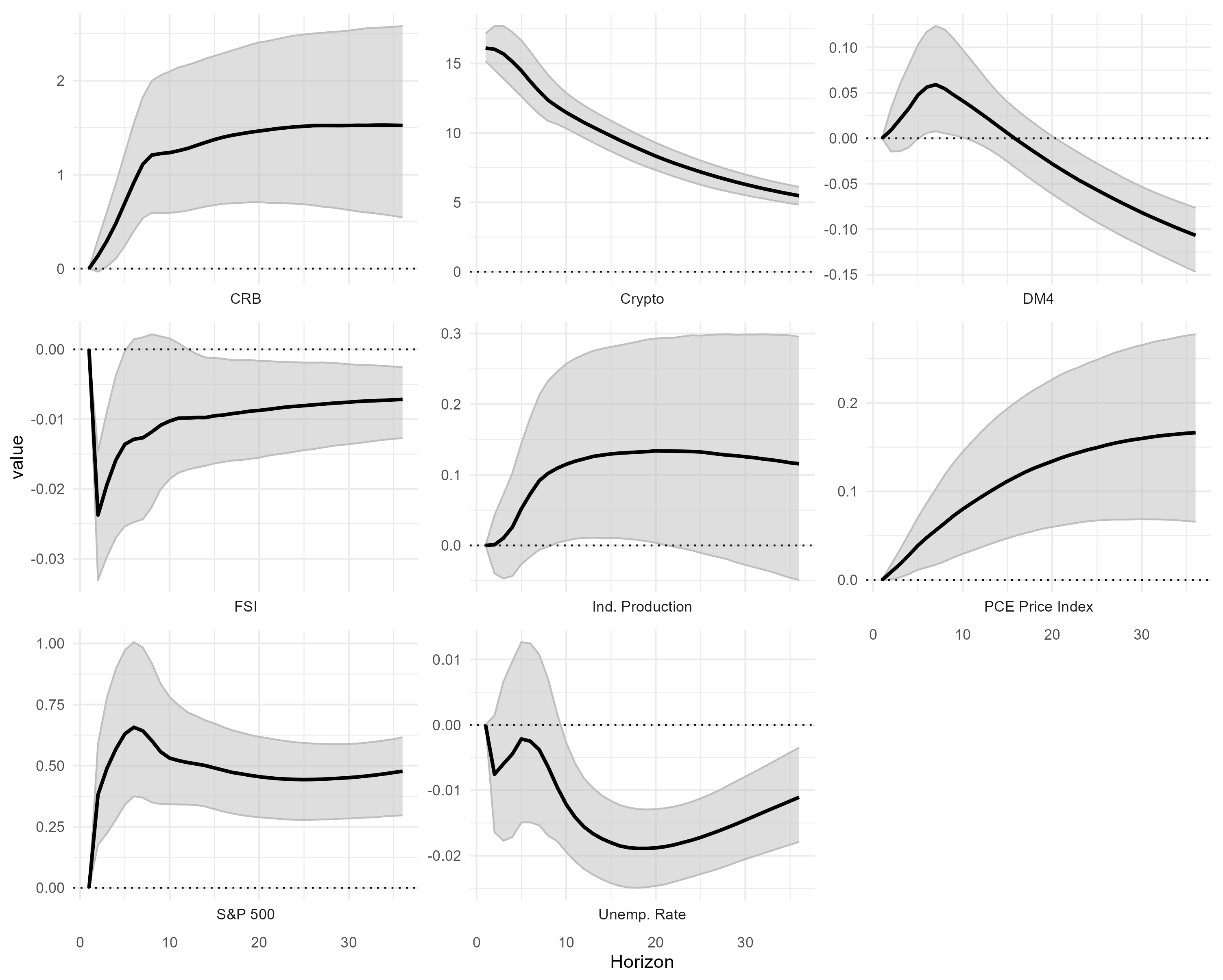
The baseline identification orders cryptocurrency price fifth in the recursive structure, implying that crypto prices do not contemporaneously respond to shocks from financial variables (S&P 500, CRB commodity index, and financial stress index). This assumption may be restrictive given the increasing integration of cryptocurrency markets with other financial markets.

To test the sensitivity to this identification assumption, the SVAR is re-estimated with cryptocurrency price ordered last in the recursive structure. This alternative ordering allows crypto prices to respond contemporaneously to all other variables in the system, including financial market innovations. Under this specification, cryptocurrency shocks represent innovations that are orthogonal to contemporaneous movements in all macroeconomic and financial variables.

Figure 2 shows the impulse response functions under the alternative ordering are virtually indistinguishable from the baseline results. Unreported tests that consider changing orders within macroeconomic variables and within financial variables generate qualitatively identical results. This robustness indicates that the main findings regarding cryptocurrency shock transmission mechanisms and macroeconomic effects are not sensitive to the specific contemporaneous restrictions imposed in the identification scheme.

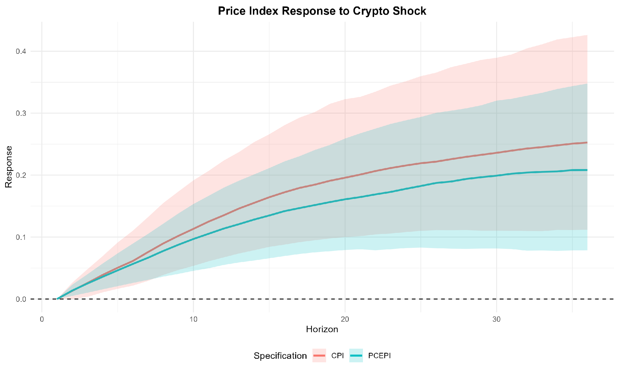
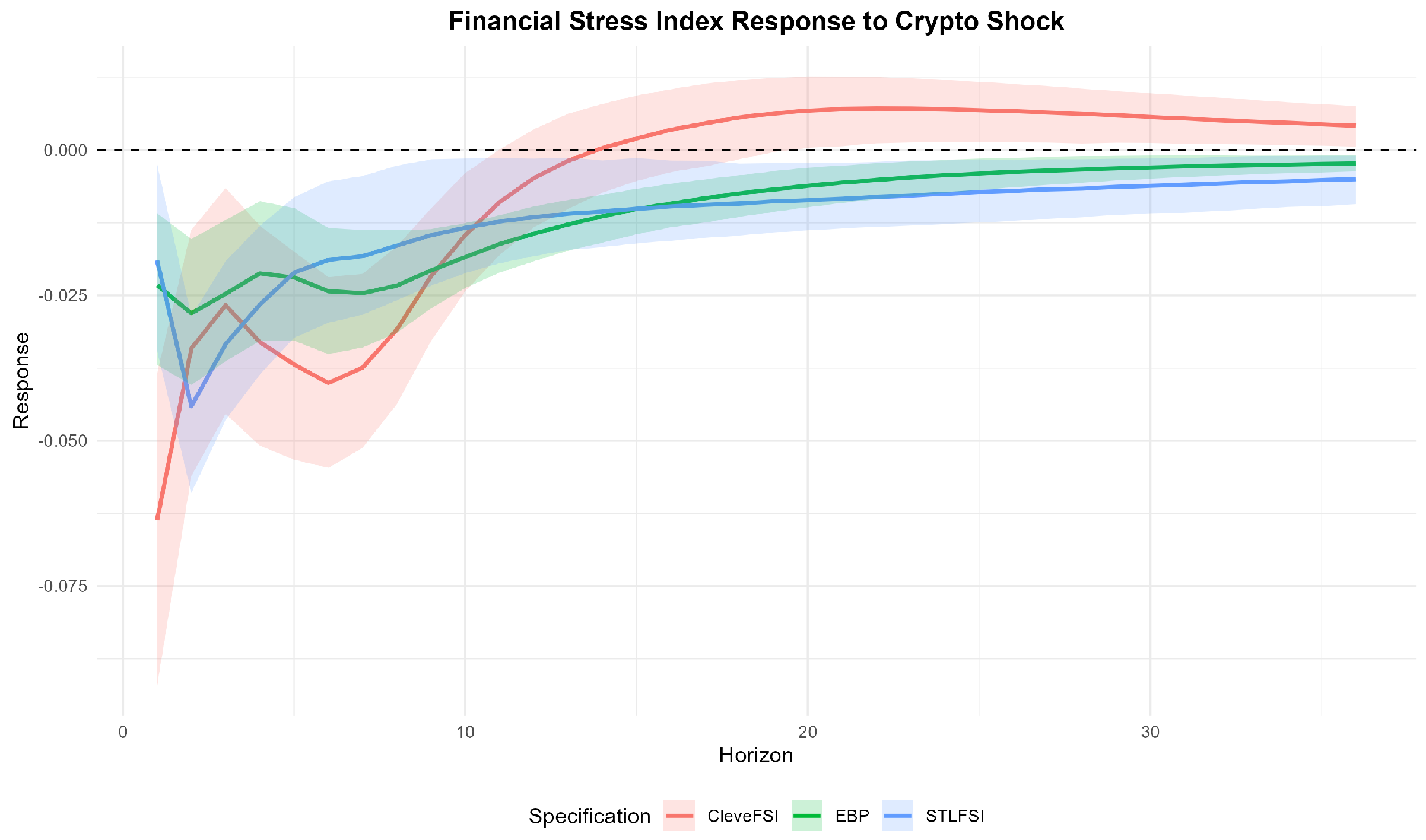
6.2. Alternative Measures of Price Level and Financial Stress

The baseline specification employs the PCE price index and St. Louis Fed Financial Stress Index as measures of inflation and financial conditions. To verify the robustness to alternative variable definitions, the SVAR is re-estimated using the CPI price index and alternative financial stress measures: the Excess Bond Premium (EBP) of Gilchrist and Zakrajšek (2012) and the Cleveland Fed Financial Stress Index.

Figure 3 and Figure 4 show that the impulse responses of price level and financial stress variables to cryptocurrency shocks remain qualitatively similar across specifications. The CPI and PCE price indices exhibit nearly identical gradual positive responses to crypto shocks, confirming that the inflation findings are robust to the choice of price measure. Similarly, all three financial stress indicators—St. Louis FSI, EBP, and Cleveland FSI—display comparable initial declines followed by gradual recovery patterns, indicating that cryptocurrency shocks consistently reduce financial stress across different measures of financial market conditions. This robustness validates the baseline results and demonstrates that the documented transmission mechanisms are not artifacts of specific variable choices.

6.3. Alternative Pandemic Prior Setting

The Pandemic Priors methodology involves a key hyperparameter $\varphi$ that controls the tightness of the prior distribution around the pandemic-period relationships. The baseline specification uses the optimally selected $\varphi =0.1$, chosen via grid search over 25 values ranging from 0.001 to 500, based on marginal likelihood maximization. This optimally selected value indicates moderate shrinkage for the pandemic dummy coefficients.

A specification is estimated with strong beliefs that COVID-19 had no substantial effects on structural relationships by setting $\varphi =500$. This prior is essentially the Minnesota prior, where Pandemic periods are treated equally as the rest of the sample. Figure 5 shows a less persistent decline in unemployment, a less persistent reduction in industrial production, and more contractionary DM4 movement in response to a positive cryptocurrency shock. This confirms that assumptions about pandemic-period structural changes can meaningfully affect the estimated transmission mechanisms of cryptocurrency shocks to macroeconomic variables and thus the Minnesota prior is inappropriate for this sample spanning the Pandemic. Meanwhile, the results in the paper, except those for the real economy, are qualitative robust to the tightness setting of the Pandemic prior.

7. Conclusions

This analysis provides empirical evidence, challenging the outdated view that cryptocurrency markets operate in isolation from financial and macroeconomic systems. The notable spillover effects from cryptocurrency price innovations are documented primarily due to its implication of overall risk appetite in financial markets and stimulus in investments.

The variance decomposition reveals that cryptocurrency shocks have become quantitatively important drivers of financial market volatility, accounting for substantial portions of equity and commodity price fluctuations. Most notably, cryptocurrency shocks explain nearly 18% of price-level forecast error variance at long horizons, suggesting they generate persistent inflationary pressures through demand-side effects.

The narrative analysis validates the structural identification and reveals that sentiment and technology shocks constitute the primary drivers of cryptocurrency market innovations. This explains why cryptocurrency shocks can transmit independently to the broader economy—they originate from sources largely orthogonal to conventional macroeconomic fundamentals.

These findings carry important implications for policy makers. Given that cryptocurrency shocks contribute 18% to long-term price variance with persistent inflationary effects, monetary policy authorities should incorporate cryptocurrency developments in forecasting and monitor these markets for demand-driven inflation pressures. Financial regulators should monitor cryptocurrency markets as systematic risk sources and distinguish sentiment-driven volatility from technology-driven value creation, as crypto shocks now account for a substantial portion of financial market variance.

The integration of cryptocurrency markets with financial and macroeconomic systems represents a fundamental shift in the global financial architecture. The dual-channel framework reveals that sentiment drives financial integration while technology drives real transmission. Rather than simply providing portfolio diversification, cryptocurrencies may now function as systematic risk amplifiers. The era of treating cryptocurrency markets as a separate, disconnected asset class may be coming to an end.

Admittedly, this analysis has several limitations. First, focusing solely on Bitcoin may not capture the heterogeneous effects across the broader cryptocurrency ecosystem. Second, the relatively short sample period limits the examination of longer-term structural relationships. Third, recursive identification imposes restrictive contemporaneous assumptions that may not reflect high-frequency market interactions. Fourth, narrative event categorization involves subjective judgment. Finally, the linear VAR framework may miss nonlinearities and regime changes in shock transmission.

Future research on cryptocurrency price shocks should prioritize a granular investigation into the dynamic impacts on various components of the economy, such as consumption, investment, income, etc. Additionally, refinement in SVAR identification—including sign restrictions, external instruments, and heteroskedasticity-based identification—could address the limitations of recursive ordering assumptions.