Article

The Nonlinear Impact of Environmental, Social, Governance on Stock Market Performance Among US Manufacturing and Banking Firms

Department of Economics, American University, Washington, DC 20016, USA
*
Author to whom correspondence should be addressed.
J. Risk Financial Manag. 2025, 18(6), 293; https://doi.org/10.3390/jrfm18060293
Submission received: 17 April 2025 / Revised: 18 May 2025 / Accepted: 19 May 2025 / Published: 28 May 2025
(This article belongs to the Section Financial Markets)

Abstract

Results of studies have varied significantly regarding the effect of ESG investment on firm value. This paper weighs in on this issue by analyzing how changes in ESG scores impact excess stock market returns (alpha) and risk-adjusted returns (Sharpe ratio). We also analyze the differential impact of ESG investments on financial performance among US manufacturing and banking firms. Using quantile regression analysis, our results show a nonlinear relationship, characterized by a U-shaped relationship between ESG ratings and alpha but an inverted U-shaped relationship between ESG and the Sharpe ratio. These findings, along with results pertaining to the impact of ESG components, help explain conflicts in the literature regarding the effect of ESG investment on firm value.

1. Introduction

While companies have reported Environmental, Social, Governance (ESG) events for many years, they did not start to disclose ESG investments until the late 2000s, or shortly after the United Nations Global Compact report. Shortly thereafter, data service companies1 started to provide a somewhat standardized method of rating companies on their ESG activities. Investors can thus assess a company’s performance and risk relative to its sustainability and governance practices. As such, ESG scores2 can be viewed as a third dimension in which investors evaluate a company for investment.
Companies have responded by devoting significant resources to detailing their ESG activities and goals. Are companies simply trying to improve their image to various stakeholders, or are there fundamental value changes that are suggested in environmental, governance, and social scores or measurements? ESG advocates have argued that higher ESG scores lead to less risk and lower costs of capital (Damodoran, 2023). So, if an asset is less risky, then the risk premium should be lower. Damodoran (2023) adds that because it is unclear whether ESG projects lead to lower risk and/or lower cost of financing, then perhaps the primary purpose of ESG is to disclose material issues. Other scholars, such as Miralles-Quirós et al. (2018) and Pierce and Aguinis (2013), have argued that the costs of ESG investment outweigh the benefits after a certain threshold of investment has been reached.
Empirical findings are equally divided. A growing body of work attributes this inconsistency to nonlinearity: Lahouel et al. (2022), Barnett and Salomon (2012), and others (see Wu & Chang, 2022), show that ESG can exhibit a U- or inverted U-shaped relation to firm performance. Yet four critical gaps remain. First, most studies still impose linear models, implicitly assuming a constant marginal effect of ESG spending. Second, prior research has centered on accounting metrics such as Tobin’s Q or ROA/ROE, thereby overlooking market-based indicators of excess return and risk-adjusted return. Third, disparate industries are commonly pooled, even though manufacturing and banking differ fundamentally in regulation, capital structure, and stakeholder scrutiny, making a one-size-fits-all ESG–value link implausible. Fourth, existing work rarely asks whether the benefits and costs of ESG vary across the performance distribution—or whether identical ESG outlays can push returns and risk in opposite directions.
The present study addresses these shortcomings by analyzing a decade-long panel of large manufacturing3 and banking companies4. We relate quarterly ESG scores to two market-based measures—excess stock returns (α) and the Sharpe ratio—and estimate nonlinear effects through quantile regression combined with the Sasabuchi–Lind–Mehlum test. This approach allows us to trace U- and inverted U-shaped patterns, and their turning points, at the 25th, 50th, 75th, and 90th percentiles, thereby capturing heterogeneity that mean regressions obscure.
Three principal insights emerge. First, the same ESG spending produces a U-shaped relationship with excess returns and an inverted U-shaped relationship with risk-adjusted returns, helping reconcile earlier mixed findings in the literature. Second, the sectoral comparison reveals a mirror-image pattern: manufacturers appear to underinvest in environmental and governance initiatives, whereas banks tend to overinvest environmentally, while governance and social investments exhibit U-shaped patterns with average scores falling below the estimated thresholds—implying scope for performance gains through either trimming or intensifying ESG efforts, depending on marginal returns. Third, by quantifying the optimal ESG level for each performance quartile and comparing it with the firm’s actual scores, we offer concrete benchmarks for managers considering whether to scale up or scale back ESG investment. Collectively, these contributions advance the ESG–value debate by providing a return-versus-risk framework, revealing distribution-sensitive nonlinearities and identifying sector-contingent investment thresholds.

2. Literature Review

Much of the research to date covering the value of ESG investing has focused on the behavior of the investor rather than the firm. That is, some investors prefer to invest in companies that have a strong ESG record. However, there has been an active debate about whether ESG improvements impact current and/or future firm valuations. Our research delves into three intertwined strands: the financial impact of ESG investments, the potential for nonlinear effects of ESG on financial performance, and the varied effects of individual ESG dimensions.

2.1. Effect of ESG Ratings on Financial Performance

The relationship between ESG ratings and financial performance can be viewed through different theoretical constructs. Christensen et al. (2022) argue that balancing all parties’ or stakeholders’ interests enhances corporate value. Similarly, legitimacy theory stresses a social contract between corporations and society, where breaches can lead to reduced consumer demand or increased regulatory pressures. There is also signaling theory, which argues that strong ESG performance reduces financing costs and increases corporate value (Richardson & Welker, 2001; Plumlee, 2015; Dunn et al., 2018), generally measured by Tobin’s Q (Kim & Kim, 2014; Wong et al., 2021). Similarly, the resource-based theory highlights the strategic use of internal resources, such as human capital, a key subcomponent of social, to gain a competitive advantage (Tensie et al., 2021).
Conversely, a strand of the literature grounded in trade-off theory—which views ESG spending as a potential misallocation of scarce corporate resources (Friedman, 1970; Aupperle et al., 1985; Devinney, 2009)—argues that excessive ESG outlays may raise operating costs and depress profitability. Recent empirical evidence is consistent with this view: Azmi et al. (2021) found a concave (inverted U) relationship between ESG activity and bank value in emerging economies. These results suggest diminishing returns once ESG investment surpasses an optimal level.
Those that are critical of ESG investments cite agency theory, which proposes that managers may engage in ESG activities to enhance their own reputations rather than boost corporate profits; the result may lead to wasted resources and diminished firm value (Miralles-Quirós et al., 2018). This dynamic is further elaborated by the “too-much-of-a-good-thing” (TMGT) meta-theory proposed by Pierce and Aguinis (2013), whereby the positive impacts of ESG initiatives can become negative when they exceed a certain threshold, as additional ESG costs surpass their benefits.
Over the past ten years, there have been several empirical studies that test these theories, as shown in the following table, which is organized by theory.
Authors (Date)TheoryESG Data SetResponse VariableResults
Christensen et al. (2022)StakeholderFirms worldwideAbsolute CARHigher levels of ESG disclosure lead to higher stock market volatility and returns.
Ahsan and Qureshi (2020)Stakeholder100 best US corporate citizen firmsTobin’s Q ESG boosts Tobin’s Q but not ROE or ROA.
Miralles-Quirós et al. (2018)Stakeholder theory-Book value/share; EPSEnvironmental practices are valued in environmentally sensitive industries.
Koundouri et al. (2022) StakeholderSTOXX Europe ESG Leaders 50Beta; D/E; ROA/ROEESG lowers equity risk and boosts ROA/ROE but not in the automotive sector.
Landi and Sciarelli (2019) StakeholderItalian companiesAbnormal returnsESG has no significant impact on abnormal returns.
(Wu & Chang, 2022)Trade-offTaiwanese firmsTobin’s QESG has half-convex effect in low-profit firms and concave effect in median/high-profit firms.
(Azmi et al., 2021)Trade-offEmerging market banksTobin’s Q/ROAESG activity boosts bank performance but with diminishing returns. Environmental-friendly projects boost bank value.
(Dunn et al., 2018)SignalingMSCI WorldBook/market, Market capLow-ESG-rated firms have higher risk/betas. Social and governance strongly linked to risk.
(Kim & Kim, 2014)SignalingHospitality sectorROA CSR investments reduce systemic risk in restaurants/casinos but not other segments.
(Richardson & Welker, 2001)SignalingCanadian firmsROEPositive relationship between social disclosures and the cost of equity.
(Wong et al., 2021)SignalingMalaysian firmsTobin’s Q/ROAESG ratings reduce cost of capital and increase Tobin’s Q.
Christensen et al. (2022) used an event study technique to assess how differences in ESG ratings impact stock market performance. They found that higher levels of ESG disclosure increase disagreements among rating agencies, leading to higher stock market volatility. Similarly, Wu and Chang (2022) found that among the 100 best US corporate citizens (firms), ESG enhances value as measured by Tobin’s Q, though the effect on accounting measures, such as ROE and ROA, is less evident. In contrast, Koundouri et al. (2022) found that ESG values do indeed have a positive impact on profitability measures, such as ROE and ROA, and also lower the firm’s stock price volatility or beta. Landi and Sciarelli (2019), however, in an earlier study, found that a change in ESG ratings does not impact abnormal returns.
Turning to trade-off theory, Wu and Chang (2022) found that firms with low Tobin’s Q will experience diminishing marginal returns to ESG to a greater extent than firms with higher Tobin’s Q. However, in the long run, the returns to ESG investment will increase, causing a U-shaped relationship between ESG and financial returns. Similarly, Azmi et al. (2021) examined the impact of ESG on bank performance. They found that ESG investments improve cash flow and efficiency but lower ROE. Their results also show that environmental projects versus investment in social or governance result in higher return. Miralles-Quirós et al. (2018), in an earlier study, also found that environmental projects add value, but only to firms in non-environmentally sensitive industries. In contrast, they found that the market positively values social and government practices in environmentally sensitive industries.
Another strand of the literature views ESG ratings as an information signal of risk and/or value. Dunn et al. (2018) explored this issue and found that ESG scores provide information that can change investors’ view of risk. Their study builds on Kim and Kim’s (2014) study of the hospitality industry; these authors found that ESG ratings lower systemic risk among restaurants and casinos. Their work builds on Richardson and Welker (2001), who studied the impact of social disclosures and found that releasing social information raises the cost of equity, at least among firms with a relatively low return on equity. As a result, they conjecture that social disclosure signals lower performance and/or higher risk. Wong et al. (2021) also examined the impact of ESG on borrowing cost, but they found that ESG certification lowers the cost of capital and raises a firm’s Tobin’s Q. Their findings suggest that obtaining ESG certification signals financial value to the firm. Conversely, Lin et al. (2023)5 caution that ESG investments may not always provide proportional returns, potentially due to increased operational costs, but Koundouriet al. (2022) countered that ESG might stabilize returns by reducing investment risk.

2.2. Literature Review on the Nonlinear Effects of Variables

Barnett and Salomon (2012) and Lahouel et al. (2022) argue that the discrepancies observed in studies examining the relationship between ESG criteria and financial performance are largely due to nonlinear, curvilinear relationships, indicating a more complex reality than previously understood. Barnett and Salomon (2012) add that a U-shaped relationship between corporate social performance and financial outcomes exists because while initial ESG efforts enhance a firm’s reputation and financial gains, overly ambitious efforts may reduce returns due to escalating costs and increasing stakeholder skepticism.
Lahouel et al. (2022) extend this discussion by suggesting that the costs associated with ESG initiatives in stimulating financial performance might follow a U or inverted U shape, depending on the trajectory of the costs and benefits curves, as depicted in Figure 1a,b below. The shape of the costs and benefits curve varies based on the level of upfront investment and the timing of the returns to this investment.
In Figure 16, Lahouel et al. (2022) show that the benefits of ESG investment (the orange line) have diminishing returns, while the costs (the blue line) accelerate, indicating an inverted U-shaped curve. This inverted U curve is similar to the one postulated by Pedersen et al. (2021), with the Sharpe ratio being the measurement of financial performance. In contrast, the relationship may be characterized as a U curve as shown in Figure 1b, whereby the benefits of ESG investment are accelerating, while the ESG costs show a concave or diminishing relationship with financial performance.
These findings were further substantiated by the results of Bagh et al. (2024), who employed a dynamic panel model to test the effects of ESG on the sustainable growth of US and Chinese companies. Their results showed that there was initially a positive effect, but as ESG performance increased beyond a certain threshold, the effect on sustainable growth turned negative, indicating an inverse U-shaped relationship. Sun et al. (2019) had comparable results in an earlier study, but they note the negative effect does not apply to firms with high marketing capabilities. Wu and Chang (2022) also found a concave–convex relationship between ESG and firm valuation but noted the effect differs by financial performance quantile.
Moreover, many7 of the econometric studies that found an inverted U curve between ESG and financial performance used Tobin’s Q or ROA (see Lahouel et al. (2022))/ROE as the response variable. Still, others, such as Nuber et al. (2020) and Naimy et al. (2021), found a U-shaped relationship between ESG and Tobin’s Q and/or ROA in their study of German and East Asian markets, respectively. Chen et al. (2018) also found a U-shaped relationship in their study of US companies. Fuente et al. (2022) also found the inverted U-shaped relationship, which they explain by ESG and its components first enhancing value by building trust and mitigating risk; however, these firms then experience diminishing returns to risk mitigation.
Our paper builds on these studies by using excess returns and risk-adjusted returns to test the impact of ESG and its subcomponents. To the best of our knowledge, researchers have not used excess market returns as a response variable. In addition, we build on Wu and Chang’s (2022) methodology by using quantile regression to assess differences in the linear and nonlinear effects across the range of the distribution.

2.3. Differences in E, S, and G Ratings on Financial Performance

Studies by Gompers et al. (2003) and Bebchuk et al. (2013) laid the foundation for exploring the governance dimension, showing that top-tier governance was linked to positive abnormal returns in the 1990s. However, they found minimal effect with the same companies from 2000 to 2008, indicating a maturing market understanding of governance-related profitability. Similarly, Hong and Kacperczyk (2009) noted that companies with low social responsibility scores, or ‘sin’ companies, often had positive abnormal returns surrounding a rating change, pointing to complex market reactions to different ESG dimensions.
Furthering this research, Nollet et al. (2016) explored both linear and nonlinear relationships between ESG factors and return on capital. They found a negative linear correlation between CSP and return on capital but a U-shaped relationship in nonlinear models, indicating CSP’s positive long-term impact on CFP. The U-shaped relationship was only present, however, between governance and CFP, highlighting governance’s crucial role in CSR investments and its influence on the CSP-CFP relationship.
Building on these foundational studies, recent research by La Torre et al. (2020) reveals a statistically significant impact of ESG sub-indexes (environmental, social, and governance) on company stock returns, but only in a few industries, like energy and utilities, where ESG investments appear to affect profitability. When considering the nonlinearity effects of individual ESG components, El Khoury et al.’s (2023) study of Middle Eastern financial firms found that governance has a concave relationship in its effect on accounting performance (e.g., ROA), but a convex relationship with the stock market returns.
Pedersen et al. (2021) further explored these impacts through the theory of the ESG-efficient frontier, highlighting that governance typically offered ethical investment opportunities without compromising returns; they theorize that robust governance predicts strong future fundamentals. However, environmental and social dimensions proved less reliable as predictors of future value.
Teng et al. (2022) followed up with their study of the impact of ESG risk on corporate sustainable growth (SGR). Using quantile regression, they found that ESG significantly negatively affects SGR, particularly in the upper SGR quantiles, suggesting that ESG investments are a drag on profitability among strong performing firms. Furthermore, Teng et al. (2022) found that ESG risk impacts SGR to a greater extent in environmentally sensitive industries.
Most recently, Agarwala et al. (2024) found a U-shaped relationship between the overall ESG score and market performance. Further breakdown of the ESG score showed that while social and governance dimensions exhibit a positive linear relationship with all performance metrics, the environmental dimension displays a U-shaped relationship with market performance. In contrast, Bagh et al. (2024), in their study of US and Chinese firms, found that environmental and social ratings exhibit a significant, positive effect on sustainable growth. However, the effect moves from a linear to an inverted U-shaped relationship due to diminishing returns of ESG on growth.
While the literature is replete with studies covering the linear and nonlinear impact of ESG on financial performance, there is still a gap in using these methods to cover industry differences. As such, this study fills this gap by assessing the nonlinear impact of ESG ratings on both excess returns and risk-adjusted returns among manufacturing and banking firms. By studying two different industries, we disentangle the disparate effects of ESGs on financial performance, which will explain some of the conflicting results of other studies regarding the effect of ESG ratings on firm financial performance.

3. Data

The data set covers ESG ratings by company for 10 years (2013 to 2022) and includes 53 aerospace and automotive firms (manufacturing companies) and 36 large banking firms. These companies were included since they all had MSCI scores for some of the ten-year time period and had revenues greater than USD 1 billion8.
This time period covers the inception of the MSCI ESG data in 2013 through 2022, which was the last year that ESG was available when research on the project began. We chose two key parts of the manufacturing industry, aerospace and automotive, and the banking industry to compare the effect of ESG on stock market performance in a service versus manufacturing environment.
Monthly ESG ratings were taken from the MSCI database. We converted the monthly data to quarterly to match the company financial data used in our analysis. MSCI data includes monthly weighted ESG ratings, industry-adjusted ESG ratings, and separate ratings for environmental, social, and governance by company9. In addition, the data set includes ratings for ESG components, as shown in Table 1.
Environmental includes 13 issues that are organized into the course subcomponents: climate change, natural capital or resource, pollution and waste, and environmental opportunities. See ESG Ratings Methodology (msci.com) for a list of the 13 items organized into the four subcomponents that comprise the environmental rating.
Social covers health and safety, human capital development, labor management, and supply chain labor standards, which are issues in the human capital subcomponent. Social also covers consumer financial protection, privacy and data security, product safety and quality, and responsible investment, all of which are part of product liability. Lastly, social covers community relations and controversial sources that are part of stakeholder opposition, as well as access to health care and opportunities in nutrition and health that are part of social opportunities.
Corporate governance covers pay, ownership and control, and accounting, while corporate behavior includes business ethics and tax transparency.
MSCI ratings are determined by analysts who evaluate the level of risk each company faces in the three areas. Information used to arrive at the rating comes from company reports regarding their operations as well as relevant macro-level data. The rating is based on the difference between the best practices in the industry and the company’s governance, environmental, and social policies.

3.1. Variable Definitions

This paper explores how weighted average ESG ratings impacts company value, as determined by excess stock returns and risk-adjusted returns. As such, we first needed to calculate and/or estimate the response variables. To do so, we calculated the stock market return as the log difference in returns. We calculated the Sharpe ratio as the average annualized, monthly equity risk premium13 (monthly return minus the 90-day US treasury bill rate), divided by the average, annualized standard deviation of the monthly equity risk premium.
S h a r p e   r a t i o = a n n u a l i z e d   m o n t h l y   r i s k   p r e m i u m a n n u a l i z e d   m o n t h l y   s t a n d a r d   d e v i a t i o n   o f   r e t u r n s
We then estimated the quarterly alpha per company using the four factor Fama-French14 rolling regression model to estimate the constant or alpha as shown in Equation (2). The alpha or constant represents the excess return for the firm as opposed to its expected return as predicted by its benchmark, which is the four Fama French variables. To estimate alpha, we use a window of 3115 quarters and a rolling regression.
R e t u r n i t = β o + β 1 E X i t + β 2 S m b i t + β 3 H m l i t + β 4 M o m i t + + ϵ i t
In this regression return for i, t refers to the stock market return for company i in quarter t. We then used the Fama French 4 factor or Carhart (1997) model to estimate stock market returns. Ex refers to the quarterly return on the S&P 500 minus the quarterly 90-day US treasury rate or risk-free rate. Smb is the quarterly return for small minus big companies in the market, while Hml is the quarterly return for high price-to-book ratios for growth companies minus low price-to-book ratios for value companies. Finally, momentum is the return for a momentum index16 for the S&P 500.

3.2. Descriptive Statistics

Table 2 shows descriptive statistics of all variables used in the study.
In Table 2, we see the average quarterly alpha and Sharpe ratio of −0.3% and 0.06, with large standard deviations for both variables. As such, we see there is a large dispersion in the response variables, which is explained in part by differences between the manufacturing and banking sectors. We also see higher annual alpha and Sharpe ratios in the manufacturing versus banking sectors. In contrast, we find higher ESG and ESG component scores in the banking versus manufacturing sector. We will explore these relationships further in the regression analysis.

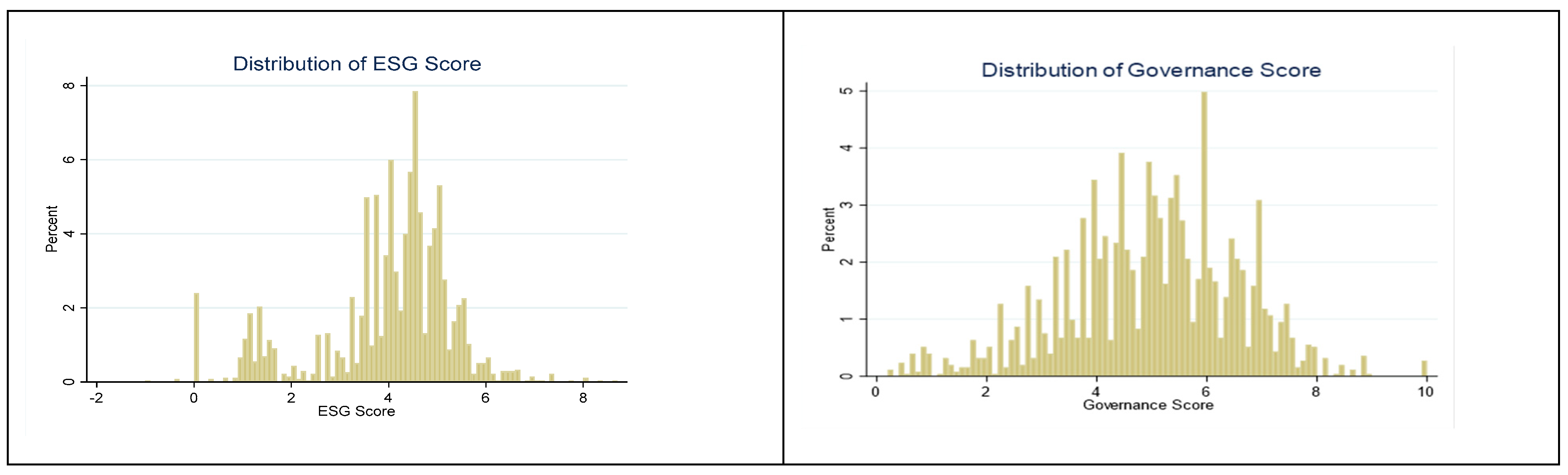
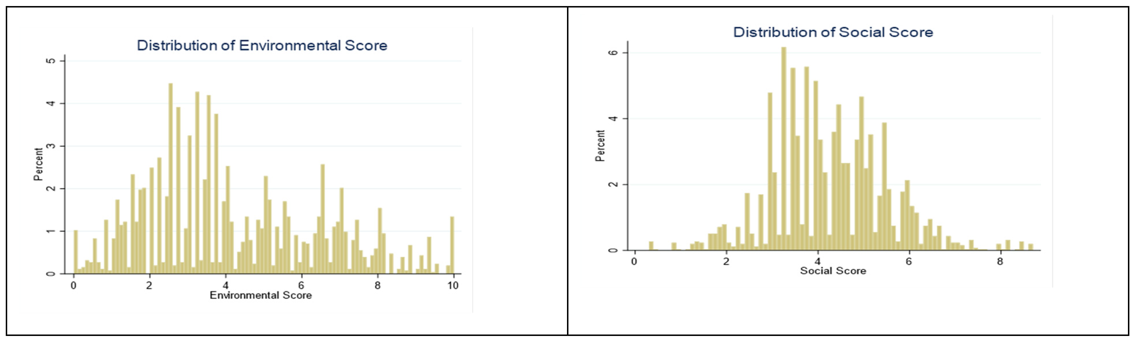
3.3. Exploratory Data Analysis

We see from from the histograms in Figure 2 that weighted ESG, governance, and social all have near-bell-shaped curves, with the highest frequency at or near their means. In contrast, the frequency of environmental scores shows a large dispersion, with the highest frequency being below the mean.
Figure 3 presents scatterplots of weighted ESG versus alpha and the Sharpe ratio.
From the figures, we see a fairly tight distribution of alpha near zero and ESG scores between 4 and 6. For the Sharpe ratio17 the distribution is also very tight around zero, with ESG scores fairly evenly dispersed between 1 and 6.
Given the dense nature of the data, the scatterplots were run again but using the lowess smoother technique, which can be advantageous in visualizing nonlinear relationships. The lowess smoother plot of alpha vs. ESG appears to be linear and negative across the distribution. For the Sharpe ratio lowess smoother plot, there appears to be an inverted U relationship, though slight, between ESG values of 2 and 6. We will explore these relationships further in the regression analysis.

4. Hypotheses

Building on the theoretical and empirical foundations discussed earlier, this section develops a testable framework to explain the complex relationship between ESG scores and firm financial performance. We first examine the overall nonlinear effect and then assess the differential effects of ESG subcomponents across two industries (manufacturing and banking), followed by the marginal effects of curve positioning.

4.1. Conceptual Foundation: Overall Nonlinear Effects of ESG on Firm Performance

Stakeholder theory and legitimacy theory suggest that moderate ESG investments enhance corporate reputation, reduce financing costs, and increase firm value (Christensen et al., 2022). Signaling theory further argues that ESG disclosures provide credible information about firm quality and lower risk, improving access to capital (Richardson & Welker, 2001; Dunn et al., 2018; Wong et al., 2021). However, agency theory and the “too-much-of-a-good-thing” (TMGT) meta-theory warn that excessive ESG spending may reflect managerial self-interest and lead to overinvestment, resulting in diminishing or even negative returns (Pierce & Aguinis, 2013; Miralles-Quirós et al., 2018). Pedersen et al. (2021) further propose that ESG acts as a third dimension in investor decision making, meaning that different measures of financial performance (e.g., excess returns vs. risk-adjusted returns) may reflect different nonlinear patterns.
Hypothesis 1:
There is a nonlinear relationship between overall ESG scores and firm financial performance. As ESG investment increases, firm performance may exhibit a U-shaped or inverted U-shaped pattern, depending on risk–return trade-offs, industry characteristics, and the performance measure used (such as excess returns or Sharpe ratio).

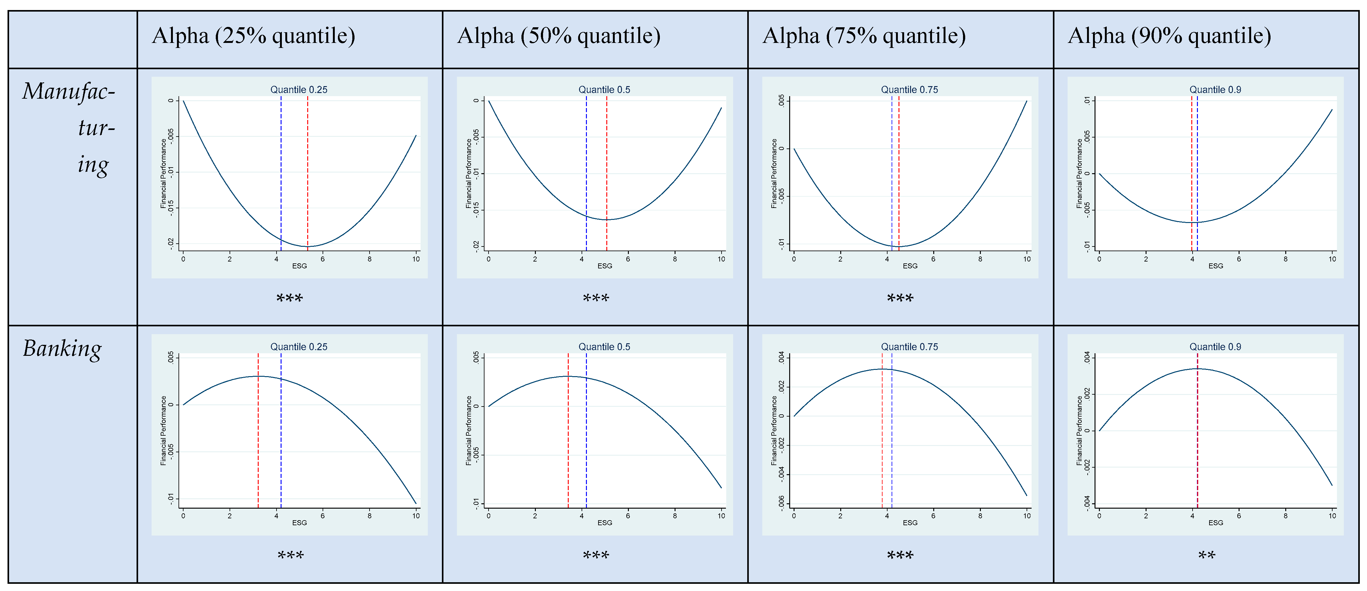
4.2. Dimension-Specific Nonlinearity in Industries

4.2.1. Manufacturing Sector—Conceptual Foundation

In capital-intensive manufacturing, large, fixed investments in governance systems (e.g., supply chain audits) and environmental improvements (e.g., emissions abatement) often generate negative returns initially before scale economies emerge, leading to a potential U-shaped relationship (Barnett & Salomon, 2012; Azmi et al., 2021). In contrast, social responsibility initiatives (such as employee safety programs or community engagement) may provide quick reputational benefits at lower cost but offer diminishing returns as stakeholder expectations are met, resulting in a possible inverted U shape (El Khoury et al., 2023).
Hypothesis 2A:
Among manufacturing firms, governance and environmental scores are expected to exhibit a U-shaped relationship with firm financial performance, while social scores are expected to show an inverted U-shaped relationship.

4.2.2. Banking Sector—Conceptual Foundation

Banking activities are highly dependent on regulatory approval and customer trust. Improvements in governance and social responsibility can reduce compliance, conduct, and reputational risks, potentially creating a U-shaped relationship between ESG and performance (Gompers et al., 2003; Pedersen et al., 2021). Environmental initiatives, however, are less directly tied to core banking activities and may result in higher costs without proportional financial benefit at higher levels of investment, implying a possible inverted U shape (Lin et al., 2023).
Hypothesis 2B:
Among banking firms, governance and social scores are expected to exhibit a U-shaped relationship with firm financial performance, while environmental scores are expected to show an inverted U-shaped relationship.

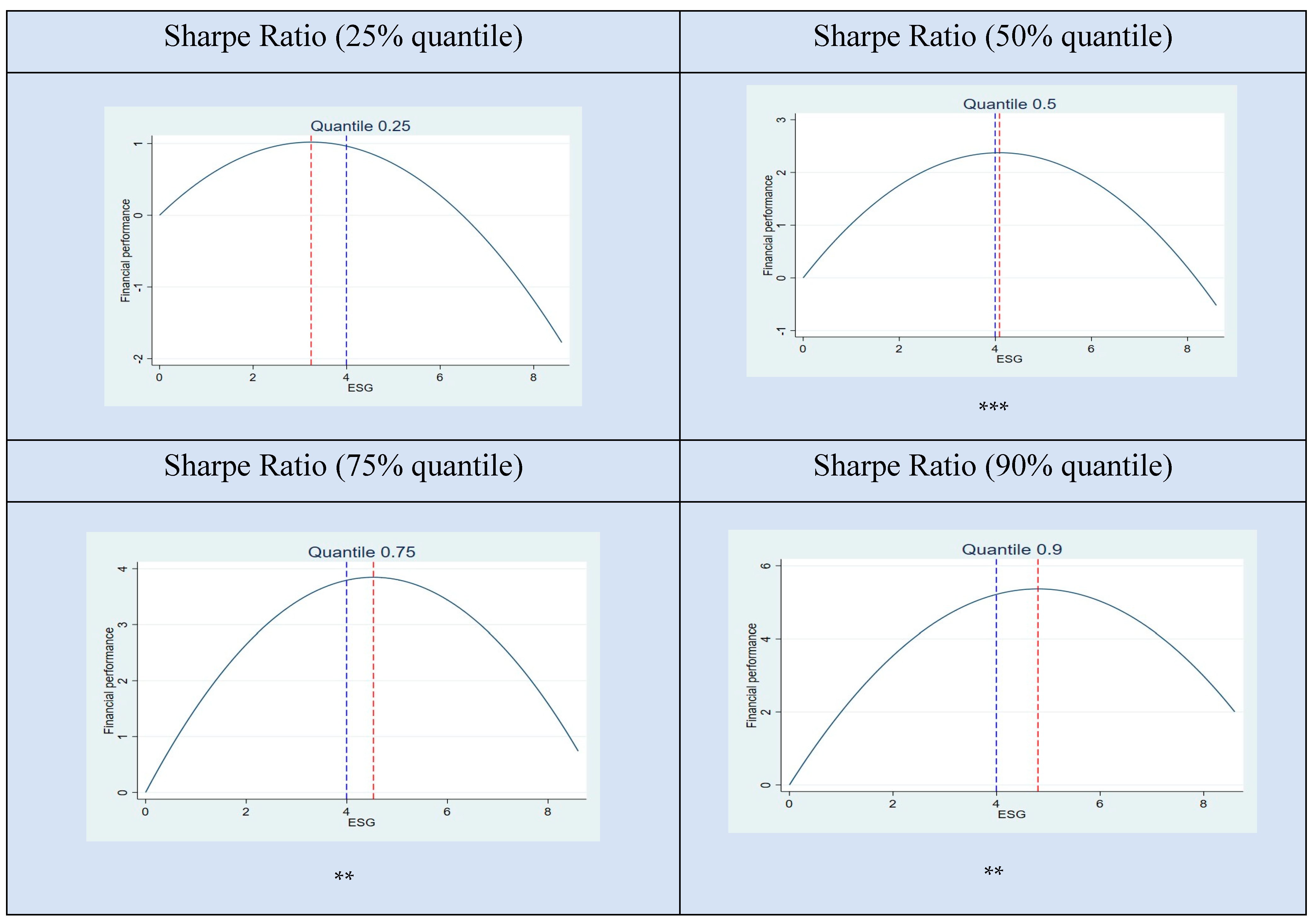
4.3. Conceptual Foundation: Marginal Effects Conditional on Curve Position

Microeconomic theory of concave and convex functions suggests that the marginal benefit of incremental ESG spending depends on the firm’s position along the curve. Firms to the left of the curve’s minimum (in a U shape) can gain from additional investment, whereas firms to the right of an inverted U-shaped peak may face diminishing or negative returns.
Hypothesis 3:
The marginal financial effect of additional ESG spending is expected to be positive for firms situated left of the U curve minimum (or left of the inverted U curve peak) and negative for firms situated right of those turning points.

5. Methodology

To test these hypotheses, we used quantile regression model(s) as shown in equations 3 through 6 below. We employed quantile regression18 to analyze the potentially nonlinear and heterogeneous effects of ESG ratings on financial performance, specifically excess returns and Sharpe ratios. This method is well suited to our research question because it accommodates the non-normal and heavy-tailed distribution often observed in financial return data. Also, it allows us to examine differences in the relationship between ESG and firm performance across the return distribution rather than assuming a constant effect as in mean-based OLS.
Our approach is also grounded in the recent literature (e.g., Wu & Chang, 2022), which has adopted quantile regression to capture similar forms of heterogeneity in ESG–performance relationships. By applying this method to our sector-specific analysis, we extend existing research and provide novel insights into the role of individual ESG dimensions in different industries. That said, we recognize the limitations of quantile regression. Estimates at the tails of the distribution (e.g., the 5th or 95th percentile) can be noisy due to small sample sizes and higher sensitivity to outliers. Moreover, the method lacks conventional model fit statistics like R-squared in OLS, making it more challenging to evaluate overall model performance or compare across quantiles. Despite these limitations, we believe quantile regression is an appropriate and effective tool for capturing the nuanced, nonlinear relationships that are central to our study.
These four equations are similar except for ESG and its squared term, as we ran separate models for each ESG subcomponent to avoid multicollinearity. See Table 3a–c for a correlation matrix19 for the total sample and both industries.20
A l p h a i t = β o + β 1 E S G i t + β 2 E S G i t 2 + β 3 R e v i t + β 4 D / E i t + β 5 I n t A i t + ϵ i t ,   Q R
A l p h a i t = β o + β 1 G i t + β 2 G i t 2 + β 3 R e v i t + β 4 D / E i t + β 5 I n t A i t + ϵ i t ,   Q R
A l p h a i t = β o + β 1 E i t + β 2 E i t 2 + β 3 R e v i t + β 4 D / E i t + β 5 I n t A i t + ϵ i t ,   Q R
A l p h a i t = β o + β 1 S i t + β 2 S i t 2 + β 3 R e v i t + β 4 D / E i t + β 5 I n t A i t + ϵ i t ,   Q R
Equations (3)–(6) were run for alpha and also for the Sharpe ratio. In addition, we segmented the sample into manufacturing and banking and showed results for each sector. ESGit refers to the weighted ESG index for company i over quarter t, while G, E, and S refer to the government, environmental, and social score for company i over quarter t, respectively. Weights for the weighted ESG index were predetermined by MSCI. We used the squared variable for ESG, E, S, and G in Equations (3)–(6) to account for the nonlinearities.
Our methodology follows the approach of Nollet et al. (2016), Fuente et al. (2022), and Wu and Chang (2022), who used a squared term in their modeling of the effect of ESG on firm financial performance.
We confirmed the presence of a U-shaped (or inverted U-shaped) relationship using the Sasabuchi–Lind–Mehlum (SLM) test (Lind & Mehlum, 2010; Sasabuchi, 1980) alongside Haans et al.’s (2016). If the Sasabuchi test statistic21 confirms a nonlinear relationship, we can then assess whether firms are under- or overinvesting in ESG and/or the ESG components by comparing the mean ESG or ESG component level to the minimum or maximum in the quartile. For the SLM test to confirm the presence of a U or inverted U-shaped relationship,
  • The coefficient β 2 in Equations (3)–(6) must be positive (for a U shape) or negative (for an inverted U shape) and statistically significant.
  • Both of the following conditions must hold:
    (a)
    The slope at the lower bound of the ESG value E S G low , calculated as β 1 + 2 β 2 . E S G low , must be significantly less than zero (for a U shape) or greater than zero (for an inverted U shape).
    (b)
    The slope at the upper bound of the ESG value ( E S G high ), calculated as β 1 + 2 β 2 . E S G high , must be significantly greater than zero (for a U shape) or less than zero (for an inverted U shape).
  • The threshold, calculated as β 1 / 2 β 2 , must lie within the data range, and the Fieller confidence interval C ^ low ,   C ^ high for the threshold lies within the data range.

6. Results and Discussion

We first estimate using quantile regression the impact of ESG ratings and ESG subcomponent ratings on the excess stock market return (alpha) and Sharpe ratio. The results using alpha and the Sharpe ratio as the response variables are shown in Table 4 and Table 5, respectively. Table 6 shows the quantile regression results by industry using alpha as the response variable. Separate regressions were run for weighted ESG, G, E, and S, with the results separated by a horizontal line in each of the Tables. The results are also shown visually in Figure 4 below, displaying the regression relationship between weighted ESG on financial performance (alpha) by quantile.
The x-axis represents weighted ESG values, and the y-axis represents financial performance (alpha). The star (s) under the figures indicate the quantile where the Sasabuchi test statistic is significant, meaning that the slopes of the initial and terminal lines are different, indicating a U or inverted U shape relationship. The red dashed line shows the ESG investment threshold or maximum/minimum level, while the blue dashed line marks the mean ESG rating by quantile. To interpret the results, we assume that ESG ratings are equivalent to investment in ESG or its subcomponent, meaning that a higher/lower rating indicates higher/lower investment.
From the results of Figure 5 and Table 4, it is clear that ESG investment impacts financial returns as shown in the significant coefficients for the linear and quadratic terms and the significant Sasabuchi test statistic in each of the quantiles. This result is somewhat consistent with Teng et al. (2022), who found ESG to negatively impact sustainable growth in the upper quantiles. We also see in Table 4 that the 95% Fieller interval for the extreme point (extremum) lies inside the specified interval, meaning we can make inferences about the U-shaped curve drawn. We also observe that in each of the quantiles, the blue lines are just left of the minimum threshold (red line), meaning that firms can either reduce their ESG investment or increase it beyond the threshold to increase financial performance.
Turning to the Sharpe ratio, as shown in Figure 6 below and Table 5, we see that in each of the quantiles for the total sample, the relationship between ESG ratings and financial performance is characterized by an inverted U-shaped relationship. The Sasabuchi test confirms the presence of a nonlinear relationship in the 50%, 75%, and 90% quartiles. Thus, when using the Sharpe ratio as the response variable, it seems that ESG investment yields positive risk-adjusted returns up to a certain point or threshold. After a certain ESG level, ESG investment actually reduces the Sharpe ratio. This finding comports with the results of Pedersen et al. (2021) suggesting a trade-off between the Sharpe ratio and ESG investment after a certain threshold has been reached.
We also see in Figure 6 that in the 75% and 90% quartiles, the blue line is left of the red line, indicating that firms are underinvesting in ESG. For the 50% quartile, the blue and red lines are located at the threshold level, suggesting firms in this quartile are investing at or near the optimal amount for ESG.
To verify the robustness of our main findings, we re-estimated the alpha using a rolling Fama French three-factor model (excluding the momentum factor), applying a 31-quarter window. This alternative measure of alpha was then used to re-run the quantile regressions. The results remain qualitatively similar—specifically, the shape of the relationship (U- or inverted U-shaped), the estimated turning points, and the relative position of the mean ESG value to the optimal threshold all exhibit only minor differences. This suggests that the observed nonlinear patterns are not driven by the inclusion of the momentum factor in the original alpha estimation.
Due to space constraints, we present a representative robustness figure using this alternative alpha measure in Appendix A Figure A2. The figure closely mirrors the patterns in the baseline analysis (Figure 5): although the result at the 25th percentile is no longer statistically significant, the U-shaped relationships remain significant at the 50th, 75th, and 90th percentiles. Moreover, the relative positioning of the ESG mean and threshold values remains consistent, further reinforcing the robustness of our findings.

6.1. Subcomponents

Moving to the subcomponents, we observe in Figure 7 below that the Sasabuchi test statistic is significant in each of the quantiles for governance ratings, and the Fieller intervals for the extreme points all lie within the specified interval for the quantiles, which supports the validity of this inference. We also see that the blue line is left of the red line in each of the quantiles, suggesting that firms are investing far less than the minimal threshold or that there are diminishing returns to investing in governance among the companies with larger excess returns. This finding fits with the results of Nollet et al. (2016), who also found a U-shaped relationship between governance and stock market performance.
This shaped relationship appears to be influenced by banking firms (See Figure 8) in the 25%, 50%, and 75% quantiles and by manufacturing in the 90% quantiles, where the Sasabuchi statistics are significant, as shown in Table 6 and Figure 8. Importantly, the Fieller intervals for the extreme points lie within the specified intervals for these quantiles, suggesting that the estimated turning points are statistically reliable. This finding provides additional support for the validity of the nonlinear relationships observed for both the banking and manufacturing sectors across the different quantiles, reinforcing confidence in the robustness of these findings.
Turning to environmental ratings, we see in Figure 7 and Table 4 that the Sasabuchi test statistic is not significant in the total sample. In addition, neither the linear coefficient nor quadratic coefficient for environmental is significant. However, in Table 6, we see the Sasabuchi test statistic is significant in the banking industry in each of the quantiles. Moreover, the Fieller interval for the extreme point (extremum) lies within the specified interval for all four quantiles, further supporting the validity of the observed nonlinear relationship in the banking sector. From Figure 8, we, therefore, can conclude that the relationship between investing in environmental in the banking industry is characterized by an inverted U curve. This indicates that beyond the turning point, banking firms experience diminishing returns from additional investments in environmental programs within these quantiles. Furthermore, we see in Figure 8 that the blue line is located just past the red line in the banking industry, suggesting that banking firms in each of the quantiles are slightly overinvesting in environmental programs. This result is consistent with the findings of Miralles-Quirós et al. (2018), who noted that environmental investment yield positive returns in non-environmentally sensitive industries, such as banking.
In contrast, the manufacturing sector shows a U-shaped relationship. For the 25%, 50%, and 75% quantiles, the blue line lies to the left of the red line with a significant Sasabuchi test statistic, indicating firms are in the diminishing returns phase. However, at the 90% quantile, the blue line lies to the right of the red line, suggesting firms have passed the turning point and are realizing positive financial returns from further environmental investments.
Finally, turning to the social rating, we see the Sasabuchi test statistic is significant in Table 4 in all quantiles, and the Fieller interval for the extreme point lies inside the specified interval in each of the quantiles. Moreover, we see in Table 6 that the Sasabuchi test statistic is significant in the manufacturing industry in all quantiles for the social regressions. These findings indicate an inverted U-shaped relationship between investing in social projects and excess returns. Furthermore, we see the blue line is left of the optimal level, suggesting increasing returns to social programs for manufacturing companies in these quantiles.
To summarize, weighted ESG ratings appear to have a nonlinear relationship with financial performance, which is characterized by a U-shaped curve relative to alpha and an inverted U-shaped relationship relative to the Sharpe ratio. Thus, there are conflicting findings based on alpha (excess return) versus the Sharpe ratio (risk-adjusted return) as to whether firms with higher financial performance should increase or reduce their ESG investments.
Governance scores had the strongest impact in the banking sector, with statistically significant U-shaped relationships observed at 25%, 50%, and 75% quantiles. In contrast, the manufacturing sector only showed significance at higher quantiles, suggesting a different sensitivity to governance across industries.
Environmental scores influenced both sectors but with different patterns: manufacturing exhibited a U-shaped relationship, while banking showed an inverted U-shaped relationship. In manufacturing, the blue line lay to the left of the turning point, suggesting firms were near the bottom of the curve, and could improve returns either by reducing or substantially increasing environmental investments. In banking, the blue line lay to the right of the turning point, indicating overinvestment and suggesting that reduced environmental spending may optimize financial returns. Both patterns were statistically significant.
The social component presented yet another pattern. In manufacturing, an inverted U shape was observed, with the red line consistently to the right of the blue line, implying underinvestment in social initiatives. In banking, a U-shaped relationship was found, with firms again positioned left of the turning point, suggesting they were near the bottom of the curve and could improve returns either by reducing or increasing social investments beyond the threshold. Finally, we see some consistent patterns for the control variables. First, the coefficient for revenue is negative and significant in Table 4, and the coefficient for intangible assets is negative and significant in Table 4 and Table 5. These results suggest that the smaller companies had better financial performance. Also, overall debt-to-equity did not appear to impact financial returns. However, we did see a negative coefficient for debt-to-equity in the 25, 50%, and 90% quantiles for banking, suggesting that a lower ratio has a positive impact for banking companies on financial returns.

6.2. Policy Implications and Recommendations

This study demonstrates that the relationship between ESG ratings and firm financial performance is nonlinear and varies by firm performance levels, ESG subcomponents, and industry contexts. The evidence of U-shaped (with excess returns, alpha) and inverted U-shaped (with risk-adjusted returns, Sharpe ratio) relationships suggests that interpreting a standard ESG score without an industry context is likely of limited value. Below, we first outline a general multi-level framework and then distill the distinct managerial and regulatory actions that flow from the manufacturing and banking results.
  • A performance- and industry-sensitive ESG framework
Because the marginal effect of ESG spending changes with (i) a firm’s position on the U or inverted U curve and (ii) its sector, both regulators and investors should replace “one-size-fits-all” checklists with tiered disclosure and assessment rules. Firms, in turn, should embed an internal return-versus-cost threshold for each E, S, and G pillar into their capital-budgeting process. In banking, where we show that high leverage erodes risk-adjusted returns, ESG criteria should also be integrated directly into risk-weighted asset and capital allocation models to avoid value-destroying overinvestment.
2.
Manufacturing (aerospace/automotive)
Our quantile regressions indicate that environmental (E) and governance (G) scores follow a U shape, while the sample mean lies left of the turning point. Most manufacturers, therefore, underinvest in energy-saving technology, supply chain audits, and board independence. By investing more in environmental and/or governance projects toward or beyond the estimated threshold, firms over time can raise both excess returns (α) and Sharpe ratios. From an investor’s perspective, equity analysts may identify alpha opportunities in manufacturing firms with low E/G scores and negative excess returns. These firms are likely to rebound once their ESG investment surpasses the optimal threshold.
The social (S) dimension displays an inverted U shape, with the mean still to the left of the peak. Additional spending on safety, employee training, and community engagement should deliver further gains, but managers must monitor marginal returns to avoid crossing the peak where benefits taper off.
Regulatory and financing levers. Industry bodies can publish process-specific carbon benchmarks, while tax credits, green-loan subsidies, and accelerated depreciation allowances should target firms that are demonstrably below the E/G efficiency threshold so that scarce green capital is not spread too thinly.
3.
Banking
For banks, the environmental score exhibits an inverted U shape, and the mean score already lies right of the peak, suggesting overinvestment in in-house environmental initiatives (e.g., low-impact premises). By contrast, both governance and social pillars show U shapes with low mean scores, signaling underinvestment in risk-control systems, board oversight, financial inclusion, and workforce diversity.
Banks should therefore rebalance their ESG budgets: trim low-yield “green showcase” projects and redirect funds toward governance and social programs that lower compliance and reputational risk, thereby improving risk-adjusted performance.
Supervisory guidance. Beyond traditional green-credit guidelines, supervisors could introduce a dual metric—an upper limit on own-operations environmental spending alongside a required minimum share of green assets—while raising capital add-ons for banks whose G or S scores remain below the industry median.

7. Conclusions

This study assesses the impact of ESG ratings on excess stock market returns and risk-adjusted returns among a group of large, US manufacturing and banking companies. The objective is to determine if investing in ESG overall and by ESG component impacts the financial performance of these companies. In our analysis, we examined both linear and nonlinear effects across performance levels and industries.
Our findings indicate that a nonlinear relationship exists between ESG ratings and financial performance. Differences emerge in the shape of the relationship, with a U-shaped relationship found when alpha is the response variable versus an inverted U-shaped relationship seen when the Sharpe ratio is the dependent variable. Furthermore, there are differences between industries in how investing in governance, environmental, and social projects impacts financial performance. In banking, governance and social scores exhibit U-shaped relationships, while environmental scores display an inverted U shape, suggesting overinvestment risks. In manufacturing, governance and environmental scores show U-shaped patterns, with firms positioned on the left side of the curve, indicating underinvestment.
This study is unique in several ways. First, we use excess returns (alpha) and risk-adjusted returns (Sharpe ratio) to measure financial performance. In doing so, we look at how ESG ratings impact both returns and risk adjusted returns. In addition, we disentangle the U- versus inverted U-shaped relationship between ESG ratings and financial performance. This is carried out by analyzing the impact of ESG ratings on financial performance (both alpha and the Sharpe ratio) overall, by industry, and by quantile. Third, we use quantile regression analysis to look at the differential, nonlinear effects of ESG and ESG components on financial performance.
To summarize, ESG ratings do appear to impact financial performance, but the relationship varies based on stock market returns of the company, the ESG component, and the industry. This study adds to the literature showing that ESG investments as reflected in ESG scores impact company value. One shortcoming of this and similar studies is using variation in stock market returns, which can be impacted by a vast array of events, as a measurement of change in value. There are other potentially more direct measurements of how firm value is impacted by ESG investments, which may include Tobin’s Q, return on assets and/or equity, merger premiums, and others. We leave it to other research to explore these relationships further and assess how investing in ESG impacts a firm’s financial performance.

Author Contributions

Conceptualization, R.S. and Y.W.; methodology, Y.W.; software, R.S. and Y.W.; validation, R.S. and Y.W.; formal analysis, R.S. and Y.W.; investigation, R.S. and Y.W.; resources, R.S.; data curation, R.S.; writing—original draft preparation, R.S. and Y.W.; writing—review and editing, R.S. and Y.W.; visualization, Y.W.; supervision, R.S.; project administration R.S.; funding acquisition, R.S. All authors have read and agreed to the published version of the manuscript.

Funding

This research received no external funding.

Institutional Review Board Statement

Not applicable.

Informed Consent Statement

Not applicable.

Data Availability Statement

Data for this study was obtained from the MSCI ESG database found in Wharton Research Services. See Wharton Research Data Services. Stock market data was obtained from the Center for Research in Security Prices CRSP) database which is also found in Wharton Research Services. See Center for Research in Security Prices, LLC (CRSP).

Conflicts of Interest

The authors declare no conflict of interest.

Appendix A

Figure A1. Alpha plotted across quantiles for social ratings in both industries. Standard errors in parentheses; *** p < 0.01, ** p < 0.05, * p < 0.1.
Jrfm 18 00293 g0a1
Figure A2. Robustness check—concave–convex effect and optimal value of weighted ESG across quantiles on alpha. Standard errors in parentheses; *** p < 0.01, ** p < 0.05, * p < 0.1.
Jrfm 18 00293 g0a2

Notes

1
Includes MSCI, S&P Global, Sustainalytics, and Refinitiv.
2
ESG ratings and scores are synonymous and refer to the numeric evaluation that a rating agency gives to the company for E, S, G, and the weighted ESG score. In contrast, ESG investment refers to the dollar amount that a company has spent in a given time period on ESG activities. ESG performance is synonymous with ESG investment.
3
Manufacturing companies are represented by aerospace and automotive companies.
4
Service companies are represented by banks.
5
Revelli and Viviani (2015) and Landi and Sciarelli (2019) also challenge the direct positive impact of ESG on stock performance.
6
Figure 1 is taken from Lahouel et al. (2022).
7
See Buallay et al. (2022) and El Khoury et al. (2023), who have found inverted U-shaped relationships in the tourism sector and banking performance in the MENAT region. Similarly, research in the Chinese market by Pu (2022) confirms the prevalence of inverted U-shaped patterns.
8
We only included larger companies because of the significant stock market volatility with smaller companies.
9
For each company, E, S, and G are weighted based on all the environmental and social key issues as well as the governance pillar score.
10
Environmental includes 13 issues that are organized into the course subcomponents: climate change, natural capital or resource, pollution and waste, and environmental opportunities. See ESG Ratings Methodology (msci.com) for a list of the 13 items organized into the four subcomponents that comprise the environmental rating.
11
Social covers health and safety, human capital development, labor management, and supply chain labor standards, which are issues in the human capital subcomponent. Social also covers consumer financial protection, privacy and data security, product safety and quality, and responsible investment, all of which are part of product liability. Lastly, social covers community relations and controversial sources that are part of stakeholder opposition, as well as access to health care and opportunities in nutrition and health that are part of social opportunities.
12
Corporate governance covers pay, ownership and control, and accounting, while corporate behavior includes business ethics and tax transparency.
13
To calculate the average annualized monthly equity risk premium, we take the average risk premium over the prior 12 months and multiply this amount by 12. The same method was applied to calculating the average, annualized standard deviation. As a result, the first Sharpe ratio entry for a firm would be in month 13, which covers the average risk premium and standard deviation for the prior 12 months.
14
We tested our results using a three-factor model (removing momentum). The results were very similar.
15
A total of 31 quarters were used for the window in the alpha estimation, as that is the average number of quarters for each company in the database.
16
This index is calculated by subtracting the equal weighted average of the lowest performing firms from the equal weighed average of the highest performing firms, lagged one month (Carhart, 1997).
17
We restricted the bottom range to -6 n the Lowess smoother figure in order to focus the data on the potential patterns. In doing so, roughly 4 Sharpe ratios were removed, but they remained in the regression analysis and summary data in Table 2.
18
See Koenker and Bassett (1978) for a discussion of quantile regression.
19
In the banking sector, there was some collinearity between intangible assets and revenues.
20
Using the Granger causality test, we also tested for reverse causality in Equations (3)–(6). In all cases, we did not find evidence to suggest reverse causality or that past values of Alpha impacted any of the ESG variables.
21
Refers to a t-statistic that evaluates whether there is a significant difference between two slopes, with one formed from the minimum X point to the minimum point on a curve versus the slope formed from the maximum X point to the minimum point on a curve.

References

  1. Agarwala, N., Jana, S., & Sahu, T. N. (2024). ESG disclosures and corporate performance: A non-linear and disaggregated approach. Journal of Cleaner Production, 437, 140517. [Google Scholar] [CrossRef]
  2. Ahsan, T., & Qureshi, M. A. (2020). The nexus between policy uncertainty, sustainability disclosure and firm performance. Applied Economics, 53(4), 441–453. [Google Scholar] [CrossRef]
  3. Aupperle, K. E., Carroll, A. B., & Hatfield, J. D. (1985). An empirical examination of the relationship between corporate social responsibility and profitability. Academy of Management Journal, 28(2), 446–463. [Google Scholar] [CrossRef]
  4. Azmi, W., Hassan, M. K., Houston, R., & Karim, M. S. (2021). ESG activities and banking performance: International evidence from emerging economies. Journal of International Financial Markets, Institutions and Money, 70, 101277. [Google Scholar] [CrossRef]
  5. Bagh, T., Zhou, B., Alawi, S. M., & Azam, R. I. (2024). ESG resilience: Exploring the non-linear effects of ESG performance on firms’ sustainable growth. Research in International Business and Finance, 70(Pt A), 102305. [Google Scholar] [CrossRef]
  6. Barnett, M. L., & Salomon, R. M. (2012). Does it pay to be really good? Addressing the shape of the relationship between social and financial performance. Strategic Management Journal, 33, 1304–1320. [Google Scholar] [CrossRef]
  7. Bebchuk, L. A., Cohen, A., & Wang, C. C. Y. (2013). Learning and the disappearing association between governance and returns. Journal of Financial Economics, 108(2), 323–348. [Google Scholar] [CrossRef]
  8. Buallay, A., Al-Ajmi, J., & Barone, E. (2022). Sustainability engagement’s impact on tourism sector performance: Linear and nonlinear models. Journal of Organization Change Management, 35, 361–384. [Google Scholar] [CrossRef]
  9. Carhart, M. M. (1997). On persistence in mutual fund performance. The Journal of Finance, 52(1), 57–82. [Google Scholar] [CrossRef]
  10. Chen, C. J., Guo, R. S., & Hsiao, Y. C. (2018). How business strategy in non-financial firms moderates the curvilinear effects of corporate social responsibility and irresponsibility on corporate financial performance. Journal of Business Research, 92, 154–167. [Google Scholar] [CrossRef]
  11. Christensen, G., Serafeim, G., & Sikochi, A. (2022). Why is corporate virtue in the eye of the beholder. The Case of ESG ratings. Accounting Review, 97(1), 147–155. [Google Scholar] [CrossRef]
  12. Damodoran, A. (2023, October 22). ESG is beyond redemption: May it RIP. Financial Times. Available online: https://www.ft.com/content/d4082c75-3141-4a58-935b-60a44c22897a (accessed on 1 December 2024).
  13. Devinney, T. M. (2009). Is the socially responsible corporation a myth? The good, the bad, and the ugly of corporate social responsibility. The Academy of Management Perspectives, 23(2), 44–56. [Google Scholar] [CrossRef]
  14. Dunn, J., Fitzgibbons, S., & Pomorski, L. (2018). Assessing risk through environmental, social and governance exposures. Journal of Investment Management, 16(1). [Google Scholar]
  15. El Khoury, R., Nasrallah, N., & Alareeni, B. (2023). The determinants of ESG in the banking sector of MENA region: A trend or necessity? Competitiveness Review: An International Business Journal, 33(1), 7–29. [Google Scholar] [CrossRef]
  16. Friedman, M. (1970). A theoretical framework for monetary analysis. Journal of Political Economy, 78(2), 193–238. [Google Scholar] [CrossRef]
  17. Fuente, G., Ortiz, G., & Velasco, P. (2022). The value of a firm’s engagement in ESG practices: Are we looking at the right side? Long Range Planning, 55(4). [Google Scholar] [CrossRef]
  18. Gompers, P. A., Ishii, J. L., & Metrick, A. (2003). Corporate governance and equity prices. Quarterly Journal of Economics, 118(1), 107–155. [Google Scholar] [CrossRef]
  19. Haans, R., Pieters, C., & He, Z. (2016). Thinking about U: Theorizing and testing U- and inverted U-shaped relationships in strategy research. Strategic Management Journal, 37(7), 1177–1195. [Google Scholar] [CrossRef]
  20. Hong, H., & Kacperczyk, M. (2009). The price of sin: The effects of social norms on markets. Journal of Financial Economics, 93(1), 15–36. [Google Scholar] [CrossRef]
  21. Kim, K. M., & Kim, Y. H. (2014). Corporate social responsibility and shareholder value of restaurant firms. International Journal of Hospitality Management, 40, 120–129. [Google Scholar] [CrossRef]
  22. Koenker, R., & Basset, G. (1978). Regression quantiles. Econometrica: Journal of the Econometric Society, 46(1), 33–50. [Google Scholar] [CrossRef]
  23. Koundouri, P., Pittis, N., & Plataniotis, A. (2022). The impact of ESG performance on the financial performance of European area companies: An empirical examination. Environmental Sciences Proceedings, 15(1), 13. [Google Scholar] [CrossRef]
  24. Lahouel, B. B., Zaied, Y. B., Managi, S., & Taleb, L. (2022). Re-thinking about U: The relevance of regime-switching model in the relationship between environmental corporate social responsibility and financial performance. Journal of Business Research, 140, 498–519. [Google Scholar] [CrossRef]
  25. Landi, G., & Sciarelli, M. (2019). Towards a more ethical market: The impact of ESG rating on corporate financial performance. Social Responsibility Journal, 15(1), 11–27. [Google Scholar] [CrossRef]
  26. La Torre, M., Mango, F., Cafaro, A., & Leo, S. (2020). Does the ESG index affect stock return? Evidence from the Eurostoxx50. Sustainability, 12, 6387. [Google Scholar] [CrossRef]
  27. Lin, Y., Wu, Y., Qian, L., & Lu, Z. (2023). ESG ratings and corporate value, investment returns: A controversial story and an evolving logic. Available online: https://business.sohu.com/a/712759717_121123881 (accessed on 2 March 2025).
  28. Lind, J. T., & Mehlum, H. (2010). With or without U? The appropriate test for a U-shaped relationship. Oxford Bulletin of Economics and Statistics, 72(1), 109–118. [Google Scholar] [CrossRef]
  29. Miralles-Quirós, M. M., Miralles-Quirós, J. L., & Gonçalves, L. M. V. (2018). The value relevance of environmental, social, and governance performance: The Brazilian case. Sustainability, 10(3), 574. [Google Scholar] [CrossRef]
  30. Naimy, V., El Khoury, R., & Iskandar, S. (2021). ESG versus corporate financial performance: Evidence from East Asian Firms in the industrials sector. Studies of Applied Economics, 39(3). [Google Scholar] [CrossRef]
  31. Nollet, J., Filis, G., & Mitrokostas, E. (2016). Corporate social responsibility and financial performance: A non-linear and disaggregated approach. Economic Modelling, 52, 400–407. [Google Scholar] [CrossRef]
  32. Nuber, C., Velte, P., & Hörisch, J. (2020). The curvilinear and time-lagging impact of sustainability performance on financial performance: Evidence from Germany. Corporate Social Responsibility Environmental Management, 27(6), 232–243. [Google Scholar] [CrossRef]
  33. Pedersen, L., Fitzgibbons, S., & Pomorski, L. (2021). Responsible investing: The ESG-efficient frontier. Journal of Financial Economics, 142(2), 572–597. [Google Scholar] [CrossRef]
  34. Pierce, J. R., & Aguinis, H. (2013). The too-much-of-a-good-thing effect in management. Journal of Management, 39(2), 313–338. [Google Scholar] [CrossRef]
  35. Plumlee, M. (2015). Voluntary environmental disclosure quality and firm value: Further evidence. Journal of Accounting and Public Policy, 34, 336–361. [Google Scholar] [CrossRef]
  36. Pu, G. (2022). A non-linear assessment of ESG and firm performance relationship: Evidence from China. Economic Research-Ekonomska Istraživanja, 36(1). [Google Scholar] [CrossRef]
  37. Revelli, C., & Viviani, J. L. (2015). Financial performance of socially responsible investing: What have we learned? A meta-analysis. Business Ethics: A European Review, 24(2), 158–185. [Google Scholar] [CrossRef]
  38. Richardson, A., & Welker, M. (2001). Social disclosure, financial disclosure and the cost of equity capital. Accounting, Organizations and Society, 26(7–8), 597–616. [Google Scholar] [CrossRef]
  39. Sasabuchi, S. (1980). A test of a multivariate normal mean with composite hypotheses determined by linear inequalities. Biometrika, 67(2), 429–439. [Google Scholar] [CrossRef]
  40. Sun, W., Yao, S., & Govind, R. (2019). Reexamining corporate social responsibility and shareholder value: The inverted-U-shaped relationship and the moderation of marketing capability. Journal of Business Ethics, 160, 1001–1017. [Google Scholar] [CrossRef]
  41. Teng, X., Ge, Y., Wu, K. S., Chang, B. G., Kuo, L., & Zhang, X. (2022). Too little or too much? Exploring the inverted U-shaped nexus between voluntary environmental, social and governance and corporate financial performance. Frontier Environmental Science, 10, 969721. [Google Scholar] [CrossRef]
  42. Tensie, W., Ulrich, A., Tracy, V. H., & Casey, C. (2021). ESG and financial performance. uncovering the relationship by aggregating evidence from 1000 plus studies published between 2015–2020. NYU Stern Center for Sustainable Business. [Google Scholar]
  43. Wong, W. C., Batten, J. A., Mohamed-Arshad, S. B., Nordin, S., & Adzis, A. A. (2021). Does ESG Certification add firm value? Finance Research Letters, 39, 101593. [Google Scholar] [CrossRef]
  44. Wu, K. S., & Chang, B. G. (2022). The concave-convex effects of environmental, social, and governance on high-tech firm value: Quantile regression approach. Corporate Social Responsibility Environmental Management, 29, 1527–1545. [Google Scholar] [CrossRef]
Figure 1. (a) Inverted U curve; (b) U curve.
Jrfm 18 00293 g001
Figure 2. Histogram of ESG and ESG components.
Jrfm 18 00293 g002aJrfm 18 00293 g002b
Figure 3. Scatterplot of alpha and the Sharpe ratio versus ESG.
Jrfm 18 00293 g003
Figure 4. Concave–convex effect and optimal value of weighted ESG across quantiles on alpha. *** p < 0.01,** p < 0.05, * p < 0.1.
Jrfm 18 00293 g004
Figure 5. Effect of weighted ESG across quantiles on the Sharpe ratio (total sample). Standard errors in parentheses; *** p < 0.01, ** p < 0.05, * p < 0.1.
Jrfm 18 00293 g005
Figure 6. Effect of ESG components across quantiles on alpha. Standard errors in parentheses; *** p < 0.01, ** p < 0.05, * p < 0.1.
Jrfm 18 00293 g006aJrfm 18 00293 g006b
Figure 7. Alpha plotted across quantiles for governance ratings in both industries. Standard errors in parentheses; *** p < 0.01, ** p < 0.05, * p < 0.1.
Jrfm 18 00293 g007
Figure 8. Alpha plotted across quantiles for environmental ratings in both industries. *** p < 0.01, ** p < 0.05, * p < 0.1.
Jrfm 18 00293 g008
Table 1. Listing of ESG components and subcomponents.
ESG ComponentsESG Subcomponent and Weight
Environmental10Climate change
Natural capital (natural resource)
Pollution and waste (waste management)
Environmental opportunities
Social11Human capital
Product liability
Stakeholder opposition
Social opportunities
Governance12Corporate governance
Corporate behavior
Table 2. Summary statistics.
VariableObservationsMeanStandard DeviationRange
Min, Max
Manufacturing MeanBanking
Mean
Alpha2796−0.0030.02−0.23, 0.34−0.0−0.03
Sharpe ratio21910.061.11−13, 8 0.15−0.04
% Banking22760.450.50, 1--
Weight-averaged ESG22764.11.240, 8.63.64.5
Governance22765.031.60.2, 104.75.4
Environmental22764.252.380, 104.24.3
Social22764.21.240.3, 104.34.1
Total revenue
(in millions of USD)
24715786897295, 57,77649266709
Debt/equity24710.96.8−121, 2141.10.8
Intangible assets
(in millions of USD)
2471703513,1890, 82,20577667338
Table 3. (a) Correlation matrix—total sample (obs = 2110). (b) Correlation matrix—aerospace/automotive sample (obs = 1236). (c) Correlation matrix—banking sample (obs = 874).
(a)
ESGESG2GovGov2EnvEnv2SocSoc2RevD/EInt. A
ESG1.000
ESG20.9631.000
Gov−0.113−0.1521.000
Gov2−0.153−0.1960.9881.000
Env−0.051−0.0530.7900.7761.000
Env2−0.050−0.0730.7490.7130.9341.000
Soc−0.115−0.1420.9250.9230.7300.6801.000
Soc2−0.146−0.1810.8870.8820.6400.5730.9721.000
Revenue−0.014−0.010−0.097−0.0730.081−0.025−0.098−0.0691.000
Debt/Equi−0.003−0.012−0.018−0.014−0.005−0.011−0.014−0.0130.0351.000
Int. Ass−0.011−0.029−0.046−0.033−0.049−0.017−0.029−0.024−0.410−0.0051.000
(b)
ESGESG2GovGov2EnvEnv2SocSoc2RevD/EInt. A
ESG1.00
ESG20.961.00
Gov−0.08−0.151.00
Gov2−0.10−0.170.991.00
Env−0.03−0.060.870.851.00
Env2−0.01−0.050.750.720.971.00
Soc−0.07−0.130.940.930.750.671.00
Soc2−0.10−0.160.880.860.660.560.971.00
Revenue−0.02−0.04−0.06−0.05−0.02−0.05−0.11−0.051.00
Debt/Equi0.010.010.170.02−0.01−0.01−0.01−0.020.051.00
Int. Ass−0.04−0.050.28−0.01−0.04−0.04−0.01−0.010.11−0.041.00
(c)
ESGESG2GovGov2EnvEnv2SocSoc2RevD/EIntA
ESG1.00
ESG20.991.00
Gov0.450.411.00
Gov20.420.380.971.00
Env0.310.32−0.38−0.051.00
Env20.270.28−0.35−0.070.971.00
Soc0.760.77−0.13−0.090.400.351.00
Soc20.750.78−0.13−0.090.400.350.991.00
Revenue−0.10−0.10−0.52−0.350.520.490.0130.121.00
Debt/Equi−0.03−0.02−0.12−0.160.02−0.010.010.020.091.00
Int. Ass−0.04−0.04−0.50−0.230.470.440.200.180.740.101.00
Table 4. Effect of ESG ratings on alpha—quantile regression.
25%50%75%90%
VariableAlphaAlpha6AlphaAlpha
ESG−0.010 ***−0.013 ***−0.015 ***−0.017 ***
(0.00)(0.00)(0.00)(0.01)
ESG-squared0.001 **0.001 **0.002 **0.002 **
(0.00)(0.00)(0.00)(0.00)
Total revenue −3.30 × 10⁻⁷ ***−3.13 × 10⁻⁷ ***−2.90 × 10⁻⁷ ***−2.71 × 10⁻⁷ **
(0.00)(0.00)(0.00)(0.00)
Debt/equity2.70 × 10−5−1.06 × 10⁻⁵−6.11 × 10⁻⁵−1.04 × 10⁻⁴
(0.00)(0.00)(0.00)(0.00)
Intangible assets−1.05 × 10⁻⁶ ***−7.38 × 10⁻⁷ ***−3.19 × 10−73.83 × 10−8
(0.00)(0.00)(0.00)(0.00)
Slope—low end−0.011 **−0.0131 ***−0.0159 ***−0.0182 ***
Slope—high end 0.0102 **0.012 ***0.0151 ***0.017 ***
Sasabuchi test statistic2.16 **0.0123 ***2.99 ***2.46 ***
Threshold (−β1/(2 β2))/within data range4.460/Yes4.432/Yes4.406/Yes4.391/Yes
95% Fieller interval for extreme point[3.942; 6.945][4.054; 5.323][4.017; 5.363][3.930; 5.924]
Gov−0.004 **−0.004 ***−0.005 ***−0.006 ***
(0.001)(0.001)(0.001)(0.001)
Gov-squared0.0003 **0.0004 *0.0004 ***0.0004 **
(0.00)(0.00)(0.00)(0.00)
Total revenue −3.36 × 10⁻⁷ **−3.22 × 10⁻⁷ ***−3.05 × 10⁻⁷ ***−2.91 × 10⁻⁷ **
(0.00)(0.00)(0.00)(0.00)
Debt/equity.0000−0.0001−6.00 × 10−5−0.0001
(0.00)(0.00)(0.00)(0.00)
Intangible assets−1.36 × 10⁻⁶ ***−9.74 × 10⁻⁷−4.99 × 10⁻⁷−1.14 × 10⁻⁷
(0.00)(0.00)(0.00)(0.00)
Slope—low end)−0.004 **−0.004 **−0.005 ***−0.006 **
Slope—high end 0.003 **0.003 **0.03 ***0.04 ***
Sasabuchi test statistic1.98 **2.99 ***3.09 ***2.4 **
Threshold (−β1/(2 β2)/within data range5.833/Yes5.943/Yes6.05/Yes6.11/Yes
95% Fieller interval for extreme point[3.218; 9.739][4.88; 7.28][5.09; 7.32][4.84; 8.12]
Env0.0000.0000.0000.000
(0.00)(0.00)(0.00)(0.00)
Env-squared0.00000.0000.000−3.64 × 10⁻⁶
(0.00)(0.00)(0.00)(0.00)
Total revenue −3.65 × 10⁻⁷ ***−3.55 × 10⁻⁷ ***−3.42 × 10⁻⁷ ***−3.30 × 10⁻⁷
(0.00)(0.00)(0.00)(0.00)
Debt/equity0.000−0.0000−0.0006−1.05 × 10−4
(0.00)(0.00)(0.00)(0.00)
Intangible assets−1.35 × 10⁻⁶ ***−9.83 × 10⁻⁷ ***−4.93 × 10⁻⁷−5.81 × 10⁻⁸
(0.00)(0.00)(0.00)(0.00)
Slope—low end)−0.0005−0.000--
Slope—high end 0.00070.0001--
Sasabuchi test statistic0.510.20--
Threshold (−β1/(2 β2)/within data range3.837/No1.764/No−7.604/No85.473/No
95% Fieller interval for extreme point[−Inf, Inf][−Inf, Inf][−Inf; +Inf][−Inf; +Inf]
Social0.009 ***0.008 ***0.007 **0.006
(0.00)(0.008)(0.00)(0.00)
Social-squared−0.001 ***−0.001 ***−0.001**−0.001
(0.00)(0.00)(0.00)(0.00)
Total revenue −3.70 × 10⁻⁷ ***−3.73 × 10⁻⁷ ***−3.77 × 10⁻⁷ ***−3.81 × 10⁻⁷ **
(0.00)(0.00)(0.00)(0.00)
Debt/equity1.07 × 10−5−2.94 × 10⁻⁵−7.23 × 10⁻⁵−1.17 × 10−4 *
(0.00)(0.00)(0.00)(0.00)
Intangible assets−1.32 × 10⁻⁶ ***−9.39 × 10⁻⁷ ***−5.29 × 10⁻⁷−1.05 × 10⁻⁷
(0.00)(0.00)(0.00)(0.00)
Slope—low end−0.004 **0.009 ***0.003 ***0.007 *
Slope—high end 0.004 **−0.009 ***−0.002 ***−0.007 *
Sasabuchi test statistic2.7 **3.04 **2.17 **1.31 *
Threshold (−β1/(2 β2)/within data range4.35/Yes4.962/Yes4.34/Yes4.32/Yes
95% Fieller interval for extreme point[3.905; 5.397][3.950; 5.140][3.741; 6.455][−Inf, Inf]
Observations2276227622762276
Standard errors in parentheses; *** p < 0.01, ** p < 0.05, * p < 0.1.
Table 5. Effect of ESG ratings on Sharpe ratios—quantile regression.
25%50%75%90%
VARIABLESSharpeSharpeSharpeSharpe
ESG0.6321.175 ***1.687 **2.223 **
(0.53)(0.41)(0.53)(0.80)
ESG-squared−0.0955−0.143 ***−0.187 **−0.223 **
(0.06)(0.05)(0.06)(0.09)
Total revenue −1 × 10⁻⁵−1 × 10⁻⁵−8 × 10⁻⁶−6 × 10⁻⁶
(0.00)(0.00)(0.00)(0.00)
Debt/equity0.001−0.003−0.007−0.010
(0.01)(0.01)(0.01)(0.01)
Intangible assets−8.26 × 10⁻⁵ ***−7.40 × 10⁻⁵ ***−6.50 × 10⁻⁵ **−5.60 × 10⁻⁵
(0.00)(0.00)(0.00)(0.00)
Slope—low end0.6301.162 ***1.699 ***2.236 **
Slope—high end −1.043 **−1.284 ***−1.527 **−1.770 **
Sasabuchi test statistic1.2502.59 ***2.16 **1.69 **
Threshold (−β1/(2 β2)/within data range3.238/Yes4.086/Yes4.529/Yes4.798/Yes
95% Fieller interval for extreme point[−Inf; 8.502] U [4.010; +Inf][3.211; 4.771][3.902; 6.661][4.092; 43.893]
Gov−0.1808−0.0740.3850.150
(0.16)(0.155)(0.238)(0.35)
Gov-squared0.0060.002−0.004 **−0.009 **
(0.12)(0.0157)(0.024)(0.036)
Total revenue 0.000−0.0000−8.77 × 10⁻⁶−7.11 × 10⁻⁶
(0.00)(0.00)(0.00)(0.00)
Debt/equity0.0006−0.003−0.0063−0.010
(0.01)(0.07)(0.01)(0.02)
Intangible assets−6.00 × 10⁻⁵ ***−5.00 × 10⁻⁵ **−0.000 ***−0.000
(0.00)(0.00)(0.00)(0.00)
Slope—low end--0.0380.15
Slope—high end --−0.032−0.02
Sasabuchi test statistic--0.1201.020
Threshold (−β1/(2 β2)/within data range--5.46/Yes8.77/Yes
95% Fieller interval for extreme point--[−Inf; +Inf][−Inf; +Inf]
Env0.1050.0790.0520.028
(0.12)(0.087)(0.114)(0.164)
Env-squared−0.0070.0060.013−0.019
(0.012)(0.010)(0.013)(0.018)
Total revenue 0.0000.000−8.09 × 10⁻⁶−5.76 × 10⁻⁶
(0.00)(0.00)(0.00)(0.00)
Debt/equity0.001−0.002−0.006−0.009
(0.01)(0.005)(0.01)(0.01)
Intangible assets0.0000.000−0.0001 **0.000
(0.00)(0.00)(0.00)(0.00)
Slope—low end----
Slope—high end ----
Sasabuchi test statistic----
Threshold (−β1/(2 β2)/within data range----
95% Fieller interval for extreme point----
Soc−0.34 *−0.258 ***−0.69 ***−0.083
(0.09)(0.161)(0.213)(0.32)
Soc-squared0.018 **0.009 **−0.002 *−0.012
(0.021)(0.169)(0.022)(0.03)
Total revenue −0.000−8.10 × 10⁻⁶−4.78 × 10⁻⁶−1.54 × 10⁻⁶
(0.00)(0.00)(0.00)(0.00)
Debt/equity0.002−0.002−0.006−0.010
(0.06)(0.01)(0.01)(0.00)
Intangible assets−0.001 **−5.00 × 10⁻⁵ ***−5.00 × 10⁻⁵ *−0.000
(0.00)(0.00)(0.00)(0.00)
Slope—low end----
Slope—high end ----
Sasabuchi test statistic----
Threshold (−β1/(2 β2)/within data range----
95% Fieller interval for extreme point----
Observations2191219121912191
Standard errors in parentheses; *** p < 0.01, ** p < 0.05, * p < 0.1.
Table 6. Effect of ESG ratings on alpha by industry—quantile regression.
25%25%50%50%75%75%90%90%
Mfg.BankingMfg.BankingMfg.BankingMfg.Banking
VARIABLESalphaalphaalphaalphaalphaalphaalphaalpha
ESG−0.012 **−0.004−0.013 ***−0.005 **−0.006 **−0.016 ***−0.019 ***−0.008 *
(0.00)(0.00)(0.00)(0.00)(0.00)(0.01)(0.01)(0.00)
ESG-squared0.001 **0.0000.002 ***0.0000.0000.002 ***0.002 **0.001
(0.00)(0.00)(0.00)(0.00)(0.00)(0.00)(0.00)(0.00)
Total revenue −1.57 × 10⁻⁶ ***−1.52 × 10⁻⁷ **−1.53 × 10⁻⁶ ***−1.30 × 10⁻⁷ ***−1.07 × 10⁻⁷*−1.47 × 10⁻⁶ ***−1.43 × 10⁻⁶ **0.000
(0.00)(0.00)(0.00)(0.00)(0.00)(0.00)(0.00)(0.00)
Debt/equity0.000−0.002 **0.000−0.003 ***−0.003 ***0.0000.000−0.004 ***
(0.00)(0.00)(0.00)(0.00)(0.00)(0.00)(0.00)(0.00)
Intangible assets−2.04 × 10⁻⁶ ***0.000−1.58 × 10⁻⁶ ***2.08 × 10−7 *3.39 × 10−7 ***−8.98 × 10−7 *0.0004.67 × 10−7 **
(0.00)(0.00)(0.00)(0.00)(0.00)(0.00)(0.00)(0.00)
Slope—low end−0.0123 ***-−0.0146 ***−0.005 **−0.0179 ***−0.007 ***−0.020 ***−0.008 **
Slope—high end 0.013 **-0.0152 **0.0000.018 ***0.0010.02 **0.003
Sasabuchi test statistic2.1 **-2.94 **0.0402.63 ***0.5102.14 **0.670
Threshold (−β1/(2 β2)4.178/Yes-4.211/Yes8.44/Yes4.243/Yes7.019/Yes4.260/Yes6.307/Yes
95% Fieller interval [3.384; 7.040]-[3.684; 5.257][−Inf; 5.672] U [−2.066; +Inf][3.658; 5.607][−Inf; 5.238] U [−3.267; +Inf][3.528; 6.919][−Inf; 4.802] U [0.374; +Inf]
Gov0.000−0.005 ***−0.002−0.004 ***−0.005 *−0.000−0.001 *−0.002 **
(0.00)(0.00)(0.00)(0.00)(0.00)(0.00)(0.00)(0.00)
Gov-squared0.0000.000 ***0.0000.000 ***0.000 ***0.0000.001 *0.000
(0.00)(0.00)(0.00)(0.00)(0.00)(0.00)(0.00)(0.00)
total revenue −1.83 × 10⁻⁶ ***−1.24 × 10⁻⁷ **−1.80 × 10⁻⁶ ***−1.19 × 10⁻⁷ ***−1.75 × 10⁻⁶ ***−1.15 × 10⁻⁷ **−1.71 × 10⁻⁶ ***0.000
(0.00)(0.00)(0.00)(0.00)(0.00)(0.00)(0.00)(0.00)
debt/equity3.54 × 10−5−0.002 *1.22 × 10−5−0.002 ***−2.29 × 10⁻⁵−0.003 ***−4.76 × 10⁻⁵−0.004 ***
(0.00)(0.00)(0.00)(0.00)(0.00)(0.00)(0.00)(0.00)
intangible assets−2.85 × 10⁻⁶ ***2.87 × 10⁻⁸−2.33 × 10⁻⁶ ***1.26 × 10⁻⁷−1.55 × 10⁻⁶ **2.19 × 10⁻⁷ *−1.00 × 10−63.17 × 10−7 *
(0.00)(0.00)(0.00)(0.00)(0.00)(0.00)(0.00)(0.00)
Slope—low end-−0.005 ***−0.2−0.004 ***−0.005 **−0.003 ***−0.001 **−0.002
Slope—high end -0.004 ***0.0010.003 ***0.0030.002 ***0.005 *0.005
Sasabuchi test statistic-5.57 ***0.524.78 ***1.262.4 ***1.36 *0.49
Threshold (−β1/(2 β2)-5.664/Yes7.03/Yes5.979/Yes6.19/Yes6.546/Yes6.023/Yes8.116/Yes
95% Fieller interval [−Inf; +Inf][5.103; 6.319][−Inf; +Inf][5.383; 6.762][−Inf; +Inf][5.492; 8.750][−Inf; +Inf][−Inf; 5.343] U [−0.292; +Inf]
Env−0.001 **0.002 ***−0.001 **0.002 ***0.005 ***0.0020.0000.002 *
(0.00)(0.00)(0.00)(0.00)(0.00)(0.00)(0.00)(0.00)
Env-squared0.000−0.0003 ***0.000−0.000 ***−0.000 ***0.0000.000−0.000 **
(0.00)(0.00)(0.00)(0.00)(0.00)(0.00)(0.00)(0.00)
Total revenue −1.88 × 10⁻⁶ ***−1.58 × 10⁻⁷ **−1.89 × 10⁻⁶ ***−1.50 × 10⁻⁷ ***−1.91 × 10⁻⁶ ***−1.38 × 10⁻⁷ **−1.92 × 10⁻⁶ ***0.000
(0.00)(0.00)(0.00)(0.00)(0.00)(0.00)(0.00)(0.00)
Debt/equity3.28 × 10−5−0.00213 **1.19 × 10⁻⁵−0.003 ***−2.05 × 10⁻⁵−0.00323 ***−4.08 × 10⁻⁵−0.004 ***
(0.00)(0.00)(0.00)(0.00)(0.00)(0.00)(0.00)(0.00)
Intangible assets−2.97 × 10⁻⁶ ***3.19 × 10⁻⁷ **−2.40 × 10⁻⁶ ***3.62 × 10⁻⁷ ***−1.53 × 10⁻⁶ **4.22 × 10⁻⁷ ***0.0004.72 × 10−7 **
(0.00)(0.00)(0.00)(0.00)(0.00)(0.00)(0.00)(0.00)
Slope—low end−0.001 ***0.002 ***−0.0060.002 ***−0.005 ***0.002−0.0030.001 **
Slope—high end 0.007 ***−0.004 ***0.006−0.003 ***0.006 ***−0.0030.005−0.0002 **
Sasabuchi test statistic2.70 ***2.96 ***2.73 ***3.56 ***1.36 *2.75 ***0.751.83 **
Threshold (−β1/(2 β2)5.338/Yes3.215/Yes5.0763.421/Yes4.502/Yes2.751/Yes3.967/Yes4.216/Yes
95% Fieller interval [4.074; 6.723][1.759; 4.099][3.637; 6.197][2.289; 4.201][−Inf; +Inf][2.081; 4.938][−Inf; +Inf][−2.747; 8.455]
Social0.011 ***−0.004 **0.011 ***−0.0030.011 ***0.0000.0112 **−0.002
(0.00)(0.00)(0.00)(0.00)(0.00)(0.00)(0.00)(0.00)
Social-squared−0.001 ***0.000−0.001 ***0.000−0.001 ***0.000−0.00123 **0.000
(0.00)(0.00)(0.00)(0.00)(0.00)(0.00)(0.00)(0.00)
Total revenue −1.76 × 10⁻⁶ ***−1.62 × 10⁻⁷ **−1.76 × 10⁻⁶ ***−1.39 × 10⁻⁷ ***−1.76 × 10⁻⁶ ***−1.73 × 10⁻⁶ ***−1.76 × 10⁻⁶ ***0.000
(0.00)(0.00)(0.00)(0.00)(0.00)(0.00)(0.00)(0.00)
Debt/equity0.000−0.003 ***−9.73 × 10⁻⁶−0.003 ***−4.52 × 10⁻⁵−0.0034 ***−7.61 × 10⁻⁵−0.004 ***
(0.00)(0.00)(0.00)(0.00)(0.00)(0.00)(0.00)(0.00)
Intangible assets−2.85 × 10⁻⁶ ***0.000−2.32 × 10⁻⁶ ***0.000−1.73 × 10⁻⁶ ***3.00 × 10⁻⁷ **−1.21 × 10−64.36 × 10−7 **
(0.00)(0.00)(0.00)(0.00)(0.00)(0.00)(0.00)(0.00)
Slope—low end0.011 ***−0.004 **0.011 ***−0.004 **0.011 **−0.003 *0.011 **−0.002
Slope—high end −0.0100.004 **−0.0100.0003 **−0.0100.002 *0.010 **0.001
Sasabuchi test statistic2.70 ***1.67 **3.35 ***1.67 **2.52 ***1.02 *1.76 **0.32
Threshold (−β1/(2 β2)4.528/Yes4.735/Yes4.537/Yes4.962/Yes4.548/Yes5.332/Yes4.556/Yes6.147/Yes
95% Fieller interval [4.026, 5.7][−Inf; 2.324] U [−1.288; +Inf][4.127, 5.339][3.763; 46.321][4.013, 6.033][−Inf; +Inf][3.765, 21.196][−Inf; +Inf]
Observations12481028124810281248102812481028
Standard errors in parentheses; *** p < 0.01, ** p < 0.05, * p < 0.1.
Disclaimer/Publisher’s Note: The statements, opinions and data contained in all publications are solely those of the individual author(s) and contributor(s) and not of MDPI and/or the editor(s). MDPI and/or the editor(s) disclaim responsibility for any injury to people or property resulting from any ideas, methods, instructions or products referred to in the content.

