Abstract
This paper addresses the problem of constructing optimal equity portfolios under volatile market conditions by minimizing realized volatility—an alternative risk quantifier that more accurately captures short-term market fluctuations than traditional variance-based approaches. This issue is particularly relevant for investors seeking robust risk management strategies in dynamic and uncertain environments. We propose a mathematical optimization framework that determines portfolio weights by minimizing realized volatility, subject to expected return constraints. The model is empirically validated using historical data from stocks listed in the Stock Exchange of Thailand 50 (SET50) index. Through a comparative analysis of realized volatility and variance-based optimization across multiple portfolio sizes and return levels, we find that portfolios constructed using realized volatility consistently achieve higher Sharpe ratios, indicating superior risk-adjusted performance. We further introduce an efficiency metric based on the Euclidean distance between optimal portfolio weight vectors to evaluate the stability of allocations under extended investment horizons. The findings underscore the practical advantages of realized volatility in portfolio construction, offering enhanced responsiveness to market dynamics and improved performance outcomes. The novelty of this study lies in integrating realized volatility into a constrained portfolio optimization model and empirically demonstrating its superiority, thereby extending traditional mean-variance methods in both scope and effectiveness.
1. Introduction
Financial markets are inherently prone to periods of heightened volatility, which can significantly influence global economic stability and investment outcomes. Such periods underscore the critical need for robust portfolio evaluation and diversification strategies, spanning a broad spectrum of financial instruments, from short-term bonds to long-term assets like stock indices and mutual funds. Historically, market volatility, particularly in bonds, has occasionally resulted in negative returns and sharp reversals, affecting the performance of mutual funds and stock indices alike Al-Najjar et al. (2021); Jiang et al. (2022); Pástor and Vorsatz (2020). These fluctuations highlight the importance of continuous vigilance and strategic risk management across various financial instruments, each with unique risk profiles, ranging from the relative safety of bank deposits to the volatility driven by systematic risks Acharya et al. (2016).
Traditionally, variance-based quantifiers have been the dominant tool for assessing volatility in financial markets. However, recent advancements in financial methodologies, particularly those utilizing high-frequency data, have enhanced our ability to capture the complex dynamics of market behavior. A key contribution in this area is the introduction of coherent risk measures by Artzner et al. (1999), which laid the foundation for modern risk management practices. Among these advancements is the concept of realized volatility, which provides a more granular understanding of market behavior compared to traditional models. Realized volatility, by capturing daily fluctuations, offers a timely and nuanced view of market risk, enabling more effective portfolio management and risk mitigation.
This paper focuses on two core risk metrics: variance (standard deviation) and realized volatility. These quantifiers, both derived from market price data, are straightforward in their application and interpretation. Standard deviation reflects historical risk by measuring the dispersion of returns from their mean, whereas realized volatility provides a more immediate assessment of market conditions by accounting for daily price movements.
Individual investors, who often lack access to the sophisticated tools and resources available to institutional investors, are particularly susceptible during periods of market volatility. This group faces distinct challenges in managing risk and diversifying portfolios, frequently balancing rational decision-making with behavioral influences Paisarn et al. (2021); Seth et al. (2020). Research shows that individual investors tend to focus on practical, returns-oriented metrics, rather than broader market indicators Prasad et al. (2021). Additionally, there is growing interest in leveraging alternative data sources, such as Google search trends, to predict market downturns during heightened volatility, underscoring the need for more strategic and adaptive risk management approaches in varying market conditions Smales (2021).
Mathematical models play an integral role in addressing the complexities of portfolio optimization, especially in the face of market volatility. These models provide a structured approach to balancing the trade-off between maximizing returns and minimizing risk, which becomes particularly important during periods of economic uncertainty. Studies have shown that diversification strategies, such as the application of Markowitz portfolio theory, are highly effective in managing risk across various markets, including the ASEAN region during periods of growth Singvejsakul et al. (2019). In addition, advanced techniques like copula models have been utilized to analyze risk, return, and diversification in specific stock markets, offering valuable insights into index performance Chaiwuttisak (2023); Thongkairat and Yamaka (2021).
The relevance of realized returns and volatility in financial stability and portfolio optimization is further underscored by studies of S&P 500 stocks during crisis periods, which have highlighted significant fluctuations in the beta coefficient and correlations between market indices and stock prices Akter and Nobi (2018). These findings illustrate the importance of beta as a risk quantifier and provide a foundation for the development of risk management strategies that can be applied across different markets.
Building on these insights, this paper introduces a novel mathematical framework for managing investment risk by incorporating realized volatility—a refined risk quantifier derived from daily logarithmic returns. Unlike conventional variance, which captures average deviation from historical returns, realized volatility reflects the cumulative variation in asset values over time. This path-dependent property enables it to more precisely capture short-term market fluctuations and react promptly to evolving risk conditions. As such, realized volatility offers a dynamic and responsive alternative to traditional volatility quantifiers, particularly valuable during periods of market turbulence or structural shifts.
Although variance-based portfolio optimization has served as the foundation of modern portfolio theory since the pioneering work of Markowitz, it is based on the assumption of constant volatility and typically relies on historical data aggregated over extended periods. This approach may result in delayed recognition of market instability. In contrast, realized volatility—motivated by continuous-time finance and supported by the theory of quadratic variation—offers superior granularity and responsiveness. Foundational studies by Andersen et al. (2003); Barndorff-Nielsen and Shephard (2002); Corsi (2009) have shown the effectiveness of realized volatility in capturing dynamic patterns of market uncertainty, leading to its growing use in volatility modeling, forecasting, and portfolio management.
In this study, we extend the use of realized volatility to a constrained portfolio optimization framework. We develop an approach that aims to minimize portfolio volatility risk—quantified through realized volatility—while ensuring a targeted expected return and compliance with portfolio allocation constraints. Our empirical application focuses on stocks listed in the SET50 index, representing a real-world setting with relatively high market volatility. In such environments, the responsiveness of realized volatility makes it especially suitable for portfolio construction. In addition to analyzing portfolio risk, we evaluate performance using the Sharpe ratio, a standard measure of risk-adjusted return. This allows for a direct comparison between realized volatility– and variance-based optimization approaches in terms of investment efficiency.
It is important to note that, while our optimization model focuses on minimizing volatility-related risk for a given target return, it remains consistent with the foundational ideas of the Markowitz framework. Rather than solving a multi-objective problem that simultaneously maximizes return and minimizes variance, we adopt a single-objective formulation with a return constraint. This approach is analytically tractable and widely accepted in the literature. By varying the return constraint, one can trace out a family of efficient portfolios that collectively form the efficient frontier. Hence, the spirit of Pareto optimality central to Markowitz’s theory is preserved, even though the optimization is structured around a fixed-return setting.
To evaluate the effectiveness of the proposed approach, we compare it with the classical variance-based optimization model. The assessment considers not only portfolio composition and allocation stability but also risk-adjusted performance via the Sharpe ratio. By computing Sharpe ratios for portfolios generated under each framework, we demonstrate that realized volatility–based portfolios consistently yield superior returns per unit of risk across all return targets and portfolio sizes. In addition, we introduce an efficiency metric based on the Euclidean distance between optimal weight vectors to assess the stability of portfolio allocations when the investment horizon is extended. This metric quantifies how resilient each risk quantifier is to new information, offering further insight into the robustness and consistency of the resulting portfolios under real-world rebalancing scenarios.
Our results indicate that portfolios constructed using realized volatility consistently demonstrate greater adaptability in asset allocation, superior Sharpe ratios, and higher stability under extended evaluation periods—particularly over short- to medium-term investment horizons. These outcomes reinforce the theoretical foundations of realized volatility and highlight its effectiveness as a forward-looking, resilient risk quantifier. Importantly, the proposed framework is not intended to replace traditional variance-based approaches but to serve as a complementary tool. By enhancing sensitivity to market fluctuations while maintaining analytical simplicity, our model offers practical value to portfolio managers seeking to balance precision with interpretability in dynamic financial environments.
This study contributes to the existing literature in several distinct ways. First, while prior works have applied realized volatility in forecasting and modeling contexts, its systematic integration into a constrained portfolio optimization framework—directly compared against variance within an emerging market setting—remains underexplored. Second, we introduce a normalized Euclidean distance–based efficiency metric to evaluate the stability of optimal portfolio weights as the investment window is extended, offering a novel perspective on portfolio robustness that is both model-agnostic and operationally intuitive. Third, our empirical analysis on SET50 constituents provides new insights into asset selection behavior under competing risk quantifiers, including firm-level interpretations and selection frequency patterns, which are rarely addressed in previous volatility optimization studies. These contributions distinguish our work from both traditional Markowitz-style models and recent applications of volatility measures in the ASEAN context (e.g., regime-switching models or machine learning–driven approaches), thereby offering a transparent, interpretable, and practically applicable framework for volatility-aware portfolio construction.
The remainder of this paper is organized as follows: Section 2 outlines the theoretical foundation for risk management and return optimization, detailing the mathematical models and methodologies used in this study. Section 3 presents the empirical findings from applying these models to the SET50 index, including a detailed comparison of Sharpe ratios. Section 4 concludes with key insights and potential avenues for future research.
2. Mathematical Model
Recent advances in portfolio optimization have increasingly focused on enhancing risk assessment methodologies, particularly through the use of high-frequency data and improved volatility estimation techniques. While traditional mean-variance optimization, introduced by Markowitz, remains a foundational model, its reliance on constant volatility and historical variance limits its responsiveness to short-term market dynamics. In response to these limitations, the concept of realized volatility has gained prominence. Seminal works such as those by Andersen et al. (2003); Barndorff-Nielsen and Shephard (2002); Corsi (2009) demonstrated the efficacy of realized volatility in capturing intraday and temporal market movements. More recent contributions have explored the use of realized quantifiers in volatility forecasting, risk management, and portfolio allocation, often highlighting their superiority in adapting to changing financial environments and in improving empirical fit.
Despite these advancements, relatively few studies have directly integrated realized volatility into constrained portfolio optimization models aimed at practical implementation for equity markets—particularly in the context of emerging markets like Thailand. This study fills this gap by developing a novel mathematical framework that leverages realized volatility to construct optimal portfolios under expected return constraints. We benchmark this approach against the classical variance-based method to demonstrate its practical and statistical advantages. In doing so, our work contributes to both the theoretical evolution and empirical applicability of volatility-based risk management tools. This section situates our model within the broader methodological landscape and sets the foundation for the mathematical formulation presented next.
Consider a scenario where n represents the number of underlying stocks in a portfolio, with denoting the spot price of stock i at time , where .
Let represent the portfolio, where each denotes the quantity of stock i held at time . In this model, is not restricted to integer values but may take any non-negative real number. This continuous setting is commonly adopted in portfolio theory and reflects practical situations in which fractional shares are allowed, such as through proportional allocations, synthetic positions, or large institutional portfolios where trading units can be split finely.
The value of portfolio X at time t is defined as follows:
Assuming an initial capital at time , we set . Consequently, the value of portfolio X can be expressed in terms of the portfolio weights as follows:
where the relationship between X and W is given by the following:
The weights satisfy the following constraints:
and
The proposed model can also accommodate scenarios where short selling is allowed, indicated with . In such cases, the constraint (3) would be modified to . However, for the sake of clarity and ease of interpretation, this paper will focus on the case where short selling is excluded.
Let be an integer representing the number of trading days, and consider the sequence of portfolio values , where . In this study, we introduce two new approaches to measuring the risk of an investment portfolio, detailed in the subsequent subsections.
2.1. Risk Quantifier Based on Variance of Percentage Returns
Consider a portfolio, X, held from time with an initial investment, . At a subsequent time, , where , the portfolio is liquidated. The percentage return of portfolio X on day j relative to is defined as follows:
Here, quantifies the profit or loss from the sale of portfolio X on day j, which may be positive, negative, or zero.
The average percentage return of portfolio X over m trading days is given by the following:
where m denotes the final trading day, , on which the position is intended to be closed.
2.2. Risk Quantifier Based on Realized Volatility
To construct a path-sensitive quantifier of portfolio risk, we adopt realized volatility, computed from logarithmic returns. First, we define the cumulative logarithmic return of portfolio X at time as follows:
where is the value of the portfolio on day j, and is the initial investment at time . This expression captures the cumulative return up to day j, accounting for compounding effects and enabling a continuous-time interpretation of return evolution.
To evaluate risk over the investment horizon, we derive daily logarithmic returns as the first differences of the cumulative log-returns, i.e., . These differences correspond to the logarithmic return of the portfolio from day j to day , consistent with the following definition:
We then compute the realized volatility of portfolio X over m trading days by aggregating the squared daily log-returns as follows:
This formulation is widely used in empirical finance as a non-parametric estimate of return variability and serves as a discrete approximation of the quadratic variation in continuous-time financial models. It provides a more granular and timely quantifier of risk than the standard deviation of cumulative returns, particularly in environments characterized by frequent price changes and short-term volatility clustering.
2.3. Determining the Optimal Portfolios Using and
2.4. Comparison of the Two Risk Quantifiers
The two risk quantifiers employed in this study—variance of percentage returns and realized volatility of logarithmic returns —capture distinct dimensions of portfolio risk and are based on fundamentally different assumptions. A systematic comparison between them reveals why realized volatility, although less traditional in classical portfolio theory, offers a more robust and effective tool for capturing short-term risk dynamics.
The risk quantifier , as defined in (7), quantifies the dispersion of percentage returns around their sample mean over a historical window of m trading days. This approach is intuitive and widely used in traditional portfolio theory, where risk is typically equated with return variability. However, it has two main limitations: (i) it relies on the assumption that returns are symmetric and linearly additive over time, and (ii) it may underrepresent compounding and nonlinear effects that are critical in high-volatility or high-frequency environments.
By contrast, realized volatility , defined in (9), measures the cumulative variation of logarithmic returns, capturing the actual pathwise movement of portfolio values. From a stochastic modeling perspective, the realized variance (the square of realized volatility) approximates the quadratic variation of the underlying asset price process, in line with the foundations of modern continuous-time finance. Under weak regularity conditions, the realized variance converges in probability to the quadratic variation for any semimartingale as the sampling interval decreases. Christensen and Podolskij (2007) developed probabilistic laws governing this convergence. For additional theoretical results, see Rujeerapaiboon et al. (2025) for models with time-varying volatility, and Rujivan (2025) for models with jumps. From an empirical standpoint, Liu et al. (2015) compared realized variance to alternative estimators using high-frequency data and found it to be highly reliable, particularly in volatile markets.
An important structural distinction lies in the data inputs: aggregates squared deviations from the mean return, whereas captures day-to-day return fluctuations directly. This makes realized volatility far more responsive to volatility clustering and abrupt market shifts, enhancing its utility in short-horizon risk monitoring and enabling more agile portfolio rebalancing. The use of logarithmic returns further ensures time consistency and analytical tractability, consistent with the continuous compounding framework employed in most financial models.
In practical terms, realized volatility has become a central tool in financial econometrics, with applications in risk forecasting, option pricing, and asset allocation. Within the context of this study, its advantages are empirically validated through two key performance metrics. First, realized volatility–based portfolios consistently yield higher Sharpe ratios than those constructed using variance, across all portfolio sizes and return levels. This demonstrates superior risk-adjusted performance. Second, we introduce an efficiency metric based on the Euclidean distance between optimal portfolio weight vectors under baseline and extended investment horizons. Realized volatility–based portfolios exhibit greater stability under these extensions, confirming their robustness to new market information and their suitability for dynamic asset allocation.
In summary, while both and are mathematically valid measures of risk dispersion, realized volatility offers clear theoretical, empirical, and practical advantages. Its ability to capture short-term risk dynamics, align with continuous-time modeling, and deliver superior performance in both Sharpe ratios and allocation stability makes it a compelling choice for modern portfolio optimization.
2.5. Evaluating the Efficiency of and
To evaluate the efficiency and robustness of the risk quantifiers and , we extend the original optimization framework by incorporating a longer evaluation period and examining the resulting changes in optimal portfolio compositions.
Let represent an integer number of additional trading days. For , the risk quantifier is extended to by substituting m in (10) and (11) with . The optimal portfolio derived by incorporating k additional trading days for the computation of is denoted as .
Similarly, for , the risk quantifier is extended to by replacing m in (14) and (11) with , while maintaining the constraints in (12) and (13). The corresponding optimal portfolio, incorporating k additional trading days for the computation of , is denoted as .
To assess how stable the portfolio weights remain when the time horizon is extended, we introduce an efficiency metric based on the Euclidean distance between the original and extended optimal weight vectors. This metric quantifies the overall shift in allocation and is normalized by the number of assets n to maintain comparability across different portfolio sizes.
The efficiency of the model based on is measured as follows:
and similarly, the efficiency of is given by the following:
These metrics are designed to take values in the interval , where a value close to 1 indicates that the portfolio structure remains largely unchanged after the extension (high stability or “efficiency”), while a value closer to 0 suggests a significant shift in weights. In extreme cases, a value of 0 would reflect a complete reallocation of the portfolio, such as when entirely new stocks replace existing ones—possibly due to updated market information. This is not a flaw but a feature: the metric accurately captures how reactive a given risk quantifier is to new data. The Euclidean distance is particularly well suited to this purpose because it is symmetric, interpretable, and sensitive to both minor adjustments and major reallocations. Therefore, it serves as a meaningful proxy for the stability and reliability of the portfolio optimization model under evolving market conditions.
These efficiency metrics are calculated for and 30 trading days, which correspond approximately to one-and-a-half weeks, three weeks, and six weeks of trading activity, respectively. Although they do not align exactly with calendar weeks, these values were chosen to represent typical short-, medium-, and intermediate-term rebalancing horizons commonly used in empirical portfolio studies. This allows us to investigate the sensitivity of the optimization results across multiple investment horizons and evaluate how resilient and stable the proposed risk quantifiers are under realistic extensions of the investment window. By examining the resulting efficiency values, we gain valuable insights into how consistently each risk quantifier supports allocation decisions as the time horizon evolves.
3. Empirical Study
This section applies the mathematical model introduced in Section 2, focusing on optimizing risk within the SET50 stocks1. The analysis is based on historical closing price data for stocks listed in the SET50 index, covering the period from October 2019 to November 2024 (5 years), with a total of trading days2.
We construct the risk-return profile , based on percentage return variance, and the portfolio volatility quantifier , based on the realized volatility of logarithmic returns. These metrics serve as objective functions in the portfolio optimization problems defined in (10) and (14), respectively, and are subject to the constraints specified in (11) through (13). The primary goal is to determine the portfolio weights that minimize risk for a given target return level.
The numerical optimization is performed using the NMinimize[] function in MATHEMATICA, a versatile tool that supports a variety of global and local optimization methods, including differential evolution, Nelder–Mead, and interior-point algorithms. Constraints are defined symbolically within the problem formulation and passed directly to NMinimize[], ensuring strict enforcement of non-negativity, budget constraints, and the return target. We rely on MATHEMATICA’s automatic solver selection and convergence diagnostics, which have shown robust and consistent behavior across repeated runs and different market conditions in our setting.
NMinimize[] handles both the nonlinearity of the objective functions and the non-convexity introduced via the constraints effectively. To ensure numerical stability and reproducibility, input price data are preprocessed through a rigorous cleaning procedure, removing missing or anomalous values and aligning time indices across all stocks. Log-returns and percentage returns are computed from the cleaned time series, and objective functions are vectorized to enhance computational efficiency.
Upon completing the optimization, we conduct a comprehensive evaluation to assess the stability, performance, and interpretability of the two risk quantifiers. This includes comparing the resulting portfolios, analyzing efficiency across various investment horizons, and examining consistency under different return scenarios. The comparative analysis provides practical insights into how the choice of risk quantifier affects portfolio construction, particularly in the context of emerging markets such as the SET50.
This evaluation not only validates the effectiveness of the realized volatility-based approach but also illustrates the operational viability of the proposed framework. By integrating advanced risk metrics with robust numerical tools, the study bridges the gap between theoretical modeling and real-world portfolio management applications.
3.1. Managing Investment Risk Using and
This study adopts two alternative risk quantifiers to guide portfolio selection: the traditional variance-based quantifier and the realized volatility quantifier . Through a comprehensive combinatorial optimization procedure, we identify the optimal weight vectors and , which minimize portfolio risk under each respective framework, given an expected return level r and a portfolio size of n stocks.
In the variance-based approach, the optimal portfolio comprises the n stocks that yield the lowest portfolio risk quantified as , where represents the estimated variance of portfolio returns. Conversely, under the realized volatility framework, the optimal portfolio is defined as the set of n stocks minimizing , which measures the cumulative variation in returns over time, calculated from high-frequency return data or historical daily log returns.
To compare the risk-adjusted performance of these portfolios, we compute the Sharpe ratio for each optimal portfolio. The Sharpe ratio is defined as the ratio of expected return to portfolio risk, with the risk term determined by the respective quantifier:
Here, the risk-free rate is assumed to be zero, consistent with the convention for short-horizon or relative performance evaluation in emerging markets.
From a risk management standpoint, investors seeking to minimize downside exposure should consider these empirically derived optimal portfolios. By construction, they represent combinations that deliver the lowest risk for a given return threshold within the SET50 universe. This study investigates portfolio configurations for , across expected return levels ranging from 1% to 5%. The following subsections present detailed analyses of the resulting optimal portfolios and their corresponding Sharpe ratios, highlighting the comparative performance under both risk quantifiers
3.1.1. Optimal Pairs of Stocks
Table 1 and Table 2 present the optimal two-stock portfolio combinations selected from the SET50 index under two distinct risk quantification frameworks: realized volatility and traditional variance. The results show that portfolio composition is highly sensitive to the choice of risk quantifier, with different stock pairings emerging across return levels when minimizing either or .

Table 1.
Two-stock portfolios optimized under realized volatility: portfolio composition, realized volatility, and Sharpe ratios.
Table 2.
Two-stock portfolios optimized under variance: portfolio composition, variance, and Sharpe ratios.
Under the realized volatility framework, the selected stock pairs change notably with increasing return targets. The portfolio begins with (ADVANC, SCC) at a 1% return, then shifts through combinations such as (SCC, SCGP), (ADVANC, BDMS), and (AOT, INTUCH), ultimately arriving at (KCE, GULF) for a 5% return. This progression suggests that higher return goals drive the optimizer toward more cyclical or growth-oriented stocks such as KCE and GULF, despite their higher volatility levels.
In contrast, the variance-based approach exhibits less diversification across return levels. The pair (TTB, TU) is repeatedly selected at 1% and 2%, followed by (CBG, SCGP) at 3%, and (KCE, SCGP) at both 4% and 5%. This persistence suggests that variance minimization leads to more conservative, lower-variance portfolios but potentially at the expense of return diversity.
Sharpe ratio comparisons confirm the realized volatility framework’s superiority. At a 1% return target, the Sharpe ratio reaches 0.33 under realized volatility, compared to only 0.02 under variance. As r increases, the realized volatility Sharpe ratio decreases to 0.13 at 5%, yet remains above the variance-based counterpart, which stays flat at 0.02–0.03. This demonstrates the greater sensitivity of Sharpe performance to return targeting under , offering stronger trade-offs between risk and reward.
3.1.2. Optimal Triplets of Stocks
Table 3 and Table 4 present three-stock portfolios optimized under realized volatility and variance minimization. Again, portfolio composition diverges significantly depending on the risk quantifier.
Table 3.
Three-stock portfolios optimized under realized volatility.
Table 4.
Three-stock portfolios optimized under variance.
Under the realized volatility criterion, portfolio composition evolves markedly across return levels—from (ADVANC, TU, BBL) at 1%, to (SCGP, TTB, SCC), (SCGP, CBG, TTB), (CBG, KCE, SCGP), and finally (KCE, ADVANC, BGRIM) at 5%. The shifting combinations reflect the optimizer’s flexibility to integrate stocks across different industries, aiming to balance rising expected returns with manageable realized volatility.
Variance-based optimization, in contrast, results in more repetitive stock selection. (ADVANC, TU, TTB) appears at 1%, followed by (SCGP, TTB, TU), (SCGP, KCE, TU). By the 4% and 5% targets, (CBG, KCE, SCGP) is chosen twice consecutively. This repeated appearance suggests that variance-based models may overly concentrate exposure to a small set of historically low-variance assets.
The Sharpe ratios again favor the realized volatility approach. At a 1% target, realized volatility yields 0.14 versus 0.02 under variance. As return targets increase, Sharpe ratios under stabilize around 0.15–0.18, while the variance-based Sharpe ratios only modestly rise to a peak of 0.04. This contrast indicates that portfolios under realized volatility scale better with increasing return demands, maintaining favorable risk-return characteristics.
3.1.3. Optimal Combinations of Four Stocks
The optimal four-stock portfolios reported in Table 5 and Table 6 further highlight how risk quantifier selection influences asset allocation decisions across target returns.
Table 5.
Four-stock portfolios optimized under realized volatility.
Table 6.
Four-stock portfolios optimized under variance.
Under realized volatility, the portfolio begins with defensive and low-volatility assets such as (ADVANC, TU, AOT, BDMS) at 1%, then gradually incorporates growth stocks like SCGP and CBG as r increases. By 5%, the optimal combination becomes (KCE, KTC, SCGP, CBG), suggesting greater tolerance for individual stock risk in pursuit of higher returns.
Under the variance framework, the optimizer starts with (ADVANC, TU, IVL, KCE) and follows a path through recurring stocks such as KCE, SCGP, and TU. These stocks dominate selections across multiple levels, reflecting the model’s preference for stability and low historical variance.
Sharpe ratios across return levels further distinguish the two approaches. Realized volatility portfolios improve from 0.11 at 1% to 0.17 at 5%, while variance-based portfolios show only marginal gains, peaking at 0.04. The sensitivity of Sharpe performance to r is notably higher under realized volatility, suggesting its superior responsiveness to changing return objectives.
3.1.4. Optimal Combinations of Five Stocks
Table 7 and Table 8 provide five-stock portfolios under both optimization frameworks. Realized volatility continues to deliver more dynamic portfolio compositions and stronger Sharpe performance.
Table 7.
Five-stock portfolios optimized under realized volatility.
Table 8.
Five-stock portfolios optimized under variance.
Portfolios under realized volatility begin with (ADVANC, KCE, TTB, SCC, STGT) and evolve through a broader mix of growth and cyclical assets such as CBG, KCE, and BGRIM. At higher return targets, stocks like TISCO and KTC also appear, reflecting increased portfolio diversification as risk tolerance rises.
In contrast, the variance-based model begins with (ADVANC, KCE, TTB, IVL, TU) and largely retains its reliance on familiar low-variance assets, only shifting to new names like GPSC and PTTGC at the 5% level. This indicates a more conservative and rigid structure as return goals increase.
Sharpe ratios underscore the realized volatility model’s advantage. At a 1% return, it delivers a Sharpe ratio of 0.20—five times higher than the variance-based model (0.04). While both frameworks show decreasing Sharpe ratios as return targets rise, the realized volatility model retains stronger performance, ending at 0.16 versus 0.02 for variance. These results reaffirm that the realized volatility approach offers greater sensitivity and adaptability to increasing return requirements, maintaining superior risk-adjusted outcomes across portfolio sizes.
3.1.5. Stock Selection Frequency
This subsection investigates the consistency of stock selections across optimized portfolios constructed under return constraints, using two alternative risk quantifiers: realized volatility and traditional variance. Employing monthly realized volatility () as the risk quantifier, we generated 20 optimal portfolios covering various configurations—portfolio sizes to 5 and return targets to (see Table 1, Table 2, Table 3, Table 4, Table 5, Table 6, Table 7 and Table 8). We then examined how frequently each stock was selected across these portfolios, thereby identifying stocks that exhibit robustness under volatility-sensitive optimization.
As shown in Figure 1a, SCGP emerges as the most frequently selected stock, appearing in 12 of the 20 portfolios, followed by KCE with nine appearances. These results indicate that both stocks offer a favorable balance between return stability and low realized volatility, making them central components of risk-minimizing strategies. Table 9 provides further context by summarizing key attributes of these top-ranked stocks, including sector classification, SET ESG ratings, market capitalization, and selection frequency.
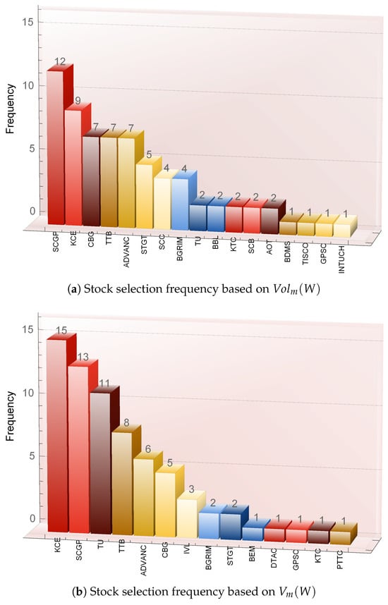
Figure 1.
Stock selection frequency based on two different risk quantifiers: realized volatility and variance. The comparison highlights the stocks most frequently selected across both risk-based methodologies, illustrating their prominence in risk-conscious investment strategies, as discussed in Section 3.1.5.
Table 9.
Top-selected stocks: sector, key financial indicators, and selection frequency (based on ).
The inclusion of SCGP and KCE can be economically rationalized. SCGP, operating in the packaging sector with a AAA ESG rating and a market capitalization exceeding 67 billion THB, benefits from demand for essential goods and strong environmental governance. These features contribute to its appeal in portfolios seeking stability and resilience. KCE, an electronics manufacturer with an A rating and smaller market capitalization, is export-oriented and offers high liquidity, which may enhance its hedging capacity against sector-specific shocks.
Other frequently selected stocks include Carabao Group (CBG), TMBThanachart Bank (TTB), and Advanced Info Service (ADVANC), each appearing in seven portfolios. CBG’s stable revenue from branded energy drink sales, both domestically and internationally, signals dependable cash flow and demand inelasticity—key attributes in volatility-averse strategies. TTB, a retail-focused bank, is known for its prudent lending policies and consistent net interest margins, making it robust during periods of financial stress. ADVANC, the market leader in telecommunications, provides recurring revenue and defensive characteristics through essential infrastructure services, reducing its exposure to macroeconomic fluctuations.
This pattern of selection underscores that high ESG ratings, diversified revenue models, and sectoral defensiveness are common traits among top-selected stocks. Importantly, these characteristics are not only reflected in their historical return behavior but are also confirmed through quantitative optimization under realized volatility.
A parallel analysis using variance as the risk quantifier produces broadly consistent results. Figure 1b reveals that KCE leads in selection frequency under the variance framework, appearing in 15 portfolios, followed closely by SCGP with 13. This consistency across both risk quantifiers reinforces the prominence of these two stocks in risk-managed strategies.
To further examine convergence across the two frameworks, we compiled the ten most frequently selected stocks under each. For realized volatility, the top selections include SCGP, KCE, CBG, TTB, ADVANC, STGT, SCC, and BGRIM, along with TU, BBL, KTC, SCB, and AOT rounding out the list. Under the variance-based framework, frequent selections include KCE, SCGP, TU, TTB, ADVANC, CBG, IVL, BGRIM, and STGT. Eight of the top ten stocks overlap across both lists, indicating an 80% concordance rate.
This high overlap suggests that despite conceptual differences—variance capturing mean dispersion and realized volatility reflecting dynamic price fluctuations—both measures converge in identifying a similar core set of stocks. These assets likely exhibit low total and idiosyncratic volatility, strong sectoral fundamentals, and stable historical performance, all of which are desirable in conservative portfolio strategies.
Overall, the results imply practical guidance for investors: consistently selected stocks—especially SCGP and KCE—serve as foundational components in portfolios designed to achieve stable, risk-adjusted returns. Their repeated inclusion across risk metrics and return targets highlights their robustness and versatility in real-world applications of volatility-based portfolio construction.
3.2. Evaluating the Efficiency of and
In this section, we evaluate the efficiency metrics and , as defined in (15) and (16), by incorporating trading periods of days into our risk optimization model. The analysis focuses on selecting n stocks from the SET50 index, with , and expected returns r ranging from 1% to 5%. These parameter choices ensure a comprehensive comparison between the efficiency of the two risk quantifiers.
Using the NMinimize[] function in MATHEMATICA, we obtain optimized portfolio weights , , , and . We then utilize the interpolation tool to generate efficiency surfaces for and , which are depicted in Figure 2a–d. The surfaces consistently lie between 0.6 and 1, indicating that both risk quantifiers yield a high degree of efficiency. However, across all evaluated scenarios, the surfaces for consistently appear closer to 1 compared to those for , suggesting that the realized volatility-based quantifier demonstrates superior efficiency relative to the variance-based quantifier .
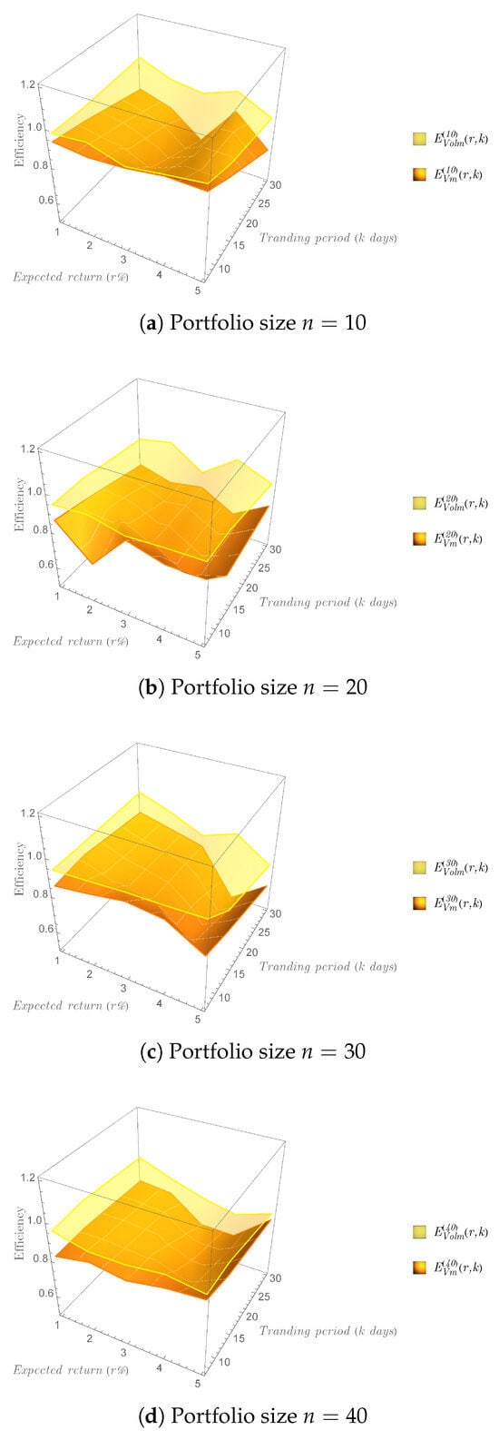
Figure 2.
Efficiency surfaces of and for various portfolio sizes n and expected returns r, incorporating additional trading periods days. Figures (a–d) compare the efficiency of the variance-based quantifier and the realized volatility-based quantifier , showing that, while both quantifiers are efficient, consistently exhibits higher efficiency across all evaluated scenarios.
As highlighted in Section 3.1.5, while both risk quantifiers provide viable strategies for constructing low-risk investment portfolios, the results presented here suggest that should be prioritized for risk evaluation due to its consistently higher efficiency. Nevertheless, it is important to acknowledge that the realized volatility-based approach does not demonstrate absolute superiority for every individual stock, as localized variations may occur. Moreover, the present study focuses on empirical analysis within the Stock Exchange of Thailand, and further validation across multiple markets would be necessary to fully generalize the findings. We leave such robustness tests for future research directions.
4. Conclusions
This study has developed a portfolio optimization framework that utilizes realized volatility as an alternative to traditional variance for quantifying risk. Rooted in the theory of quadratic variation and high-frequency return dynamics, realized volatility offers a more adaptive and time-sensitive measure of portfolio risk, particularly suited for capturing short-term market fluctuations. Applying this approach to stocks listed in the SET50 index, we conducted a comprehensive performance evaluation across multiple portfolio sizes and return targets.
The empirical results demonstrate that portfolios optimized under realized volatility consistently outperform their variance-based counterparts in terms of Sharpe ratios. Specifically, across all target return levels from 1% to 5%, realized volatility–based portfolios achieved higher risk-adjusted returns, with Sharpe ratios significantly exceeding those obtained using the variance criterion. This finding holds uniformly across portfolio sizes ranging from two to five stocks, underscoring the superior performance of realized volatility in risk-return tradeoff assessments.
Moreover, although both frameworks identified stocks such as KCE and SCGP as frequent constituents of optimal portfolios, realized volatility exhibited greater flexibility and responsiveness in portfolio composition. This reinforces its practical advantage as a more dynamic risk quantifier, capable of adjusting to market conditions in real time.
A notable contribution of this study is the systematic comparison of two widely used risk quantifiers—variance and realized volatility—within a unified optimization framework. While variance remains a foundational concept in modern portfolio theory, our findings suggest that incorporating realized volatility can significantly enhance portfolio performance by better accounting for the temporal structure of return variability. In addition, we introduced an efficiency metric based on the Euclidean distance between optimal portfolio weights to assess the robustness of allocation decisions under extended investment horizons. The results showed that realized volatility–based portfolios maintained higher allocation stability across rebalancing periods, highlighting the method’s resilience to new market information.
Importantly, the proposed framework is intended not as a replacement but as a complement to classical variance-based models. By integrating a path-dependent, high-frequency risk quantifier, the methodology bridges the gap between traditional finance theory and modern data-driven risk management practices.
In conclusion, the integration of realized volatility into portfolio optimization offers a practical and effective enhancement for managing financial risk. It enables investors to construct portfolios with improved risk-adjusted returns and greater adaptability to shifting market conditions. These insights are particularly relevant for short- to medium-term investment horizons, where responsiveness to volatility is critical.
Future research may extend this framework by incorporating additional risk dimensions, such as downside risk, tail risk, or higher moments, or by embedding it within regime-switching or multi-factor models. Such enhancements could further refine portfolio strategies in complex and volatile market environments.
Author Contributions
All authors contributed equally to the analysis and the writing of this paper. All authors have read and agreed to the published version of the manuscript.
Funding
This work was supported via the Walailak University Master’s Degree Excellence Scholarship (Contract No. CGS-ME 06/2021).
Institutional Review Board Statement
Not applicable.
Informed Consent Statement
Not applicable.
Data Availability Statement
The raw data supporting the conclusions of this article will be made available by the authors on request.
Acknowledgments
The authors would like to express their sincere gratitude to the anonymous reviewers for their constructive comments and valuable suggestions, which greatly improved the quality and clarity of this manuscript.
Conflicts of Interest
The authors declare no conflicts of interest.
Abbreviations
The abbreviations of the SET50 stocks used in this paper are as follows:
| ADVANC | ADVANCED INFO SERVICE PUBLIC COMPANY LIMITED |
| AOT | AIRPORTS OF THAILAND PUBLIC COMPANY LIMITED |
| BBL | BANGKOK BANK PUBLIC COMPANY LIMITED |
| BDMS | BANGKOK DUSIT MEDICAL SERVICES PUBLIC COMPANY LIMITED |
| BEM | BANGKOK EXPRESSWAY AND METRO PUBLIC COMPANY LIMITED |
| BGRIM | B.GRIMM POWER PUBLIC COMPANY LIMITED |
| CBG | CARABAO GROUP PUBLIC COMPANY LIMITED |
| DTAC | TOTAL ACCESS COMMUNICATION PUBLIC COMPANY LIMITED |
| GPSC | GLOBAL POWER SYNERGY PUBLIC COMPANY LIMITED |
| GULF | GULF ENERGY DEVELOPMENT PUBLIC COMPANY LIMITED |
| INTUCH | INTOUCH HOLDINGS PUBLIC COMPANY LIMITED |
| IVL | INDORAMA VENTURES PUBLIC COMPANY LIMITED |
| KCE | KCE ELECTRONICS PUBLIC COMPANY LIMITED |
| KTC | KRUNGTHAI CARD PUBLIC COMPANY LIMITED |
| PTTGC | PTT GLOBAL CHEMICAL PUBLIC COMPANY LIMITED |
| SCB | SCB X PUBLIC COMPANY LIMITED |
| SCC | THE SIAM CEMENT PUBLIC COMPANY LIMITED |
| SCGP | SCG PACKAGING PUBLIC COMPANY LIMITED |
| STGT | SRI TRANG GLOVES (THAILAND) PUBLIC COMPANY LIMITED |
| TISCO | TISCO FINANCIAL GROUP PUBLIC COMPANY LIMITED |
| TTB | TMBTHANACHART BANK PUBLIC COMPANY LIMITED |
| TU | THAI UNION GROUP PUBLIC COMPANY LIMITED |
Notes
| 1 | A list of abbreviations for the SET50 stocks is provided in this paper. |
| 2 | For details, see the Stock Exchange of Thailand’s website: https://www.set.or.th/en/market/index/set50/profile accessed between 19 October 2021 and 30 November 2024. |
References
- Acharya, V. V., Pedersen, L. H., Philippon, T., & Richardson, M. (2016). Measuring systemic risk. The Review of Financial Studies, 30(1), 2–47. [Google Scholar] [CrossRef]
- Akter, N., & Nobi, A. (2018). Investigation of the financial stability of S&P 500 using realized volatility and stock returns distribution. Journal of Risk and Financial Management, 11(2), 22. [Google Scholar]
- Al-Najjar, H., Al-Rousan, N., Al-Najjar, D., Assous, H. F., & Al-Najjar, D. (2021). Impact of COVID-19 pandemic virus on G8 countries’ financial indices based on artificial neural network. Journal of Chinese Economic and Foreign Trade Studies, 14(1), 89–103. [Google Scholar] [CrossRef]
- Andersen, T. G., Bollerslev, T., Diebold, F. X., & Labys, P. (2003). Modeling and forecasting realized volatility. Econometrica, 71(12), 579–625. [Google Scholar] [CrossRef]
- Artzner, P., Delbaen, F., Eber, J.-M., & Heath, D. (1999). Coherent measures of risk. Mathematical Finance, 9(3), 203–228. [Google Scholar] [CrossRef]
- Barndorff-Nielsen, O. E., & Shephard, N. (2002). Estimating quadratic variation using realized variance. Journal of Applied Econometrics, 17, 457–477. [Google Scholar] [CrossRef]
- Chaiwuttisak, P. (2023). Multi-criteria decision-making for investment portfolio selection in Thailand’s stock market (Volume 370 of frontiers in artificial intelligence and applications, pp. 188–196). IOS Press. [Google Scholar]
- Christensen, K., & Podolskij, M. (2007). Realized range-based estimation of integrated variance. Journal of Ecomometrics, 141, 323–349. [Google Scholar] [CrossRef]
- Corsi. (2009). A simple approximate long-memory model of realized volatility. Journal of Financial Econometrics, 7(2), 174–196. [Google Scholar] [CrossRef]
- Jiang, H., Li, Y., Sun, Z., & Wang, A. (2022). Does mutual fund illiquidity introduce fragility into asset prices? Evidence from the corporate bond market. Journal of Financial Economics, 143(1), 277–302. [Google Scholar] [CrossRef]
- Liu, L. Y., Patton, A. J., & Sheppard, K. (2015). Does anything beat 5-minute RV? A comparison of realized measures across multiple asset classes. Journal of Ecomometrics, 187, 293–311. [Google Scholar] [CrossRef]
- Paisarn, W., Chancharat, N., & Chancharat, S. (2021). Factors influencing retail investors’ trading behaviour in the thai stock market. Australasian Business, Accounting & Finance Journal, 15, 26–37. [Google Scholar]
- Pástor, Ľ., & Vorsatz, M. B. (2020). Mutual fund performance and flows during the COVID-19 crisis. The Review of Asset Pricing Studies, 10(4), 791–833. [Google Scholar] [CrossRef]
- Prasad, S., Kiran, R., & Sharma, R. K. (2021). Influence of financial literacy on retail investors’ decisions in relation to return, risk and market analysis. International Journal of Finance & Economics, 26(2), 2548–2559. [Google Scholar]
- Rujeerapaiboon, N., Rujivan, S., & Chen, H. (2025). Discounted-likelihood valuation of variance and volatility swaps. Financial Innovation, 11, 13. [Google Scholar] [CrossRef]
- Rujivan, S. (2025). Analytically pricing volatility options and capped/floored volatility swaps with nonlinear payoffs in discrete observation case under the Merton jump-diffusion model driven by a nonhomogeneous Poisson process. Applied Mathematics and Computation, 486, 129029. [Google Scholar] [CrossRef]
- Seth, H., Talwar, S., Bhatia, A., Saxena, A., & Dhir, A. (2020). Consumer resistance and inertia of retail investors: Development of the resistance adoption inertia continuance (raic) framework. Journal of Retailing and Consumer Services, 55, 102071. [Google Scholar] [CrossRef]
- Singvejsakul, J., Chaiboonsri, C., & Sriboonchitta, S. (2019). The dependence structure and portfolio optimization in economic cycles: An application in asean stock market. In H. Seki, C. H. Nguyen, V.-N. Huynh, & M. Inuiguchi (Eds.), Integrated uncertainty in knowledge modelling and decision making (pp. 161–171). Springer International Publishing. [Google Scholar]
- Smales, L. A. (2021). Investor attention and global market returns during the COVID-19 crisis. International Review of Financial Analysis, 73, 101616. [Google Scholar] [CrossRef]
- Thongkairat, S., & Yamaka, W. (2021). Risk, return, and portfolio optimization for various industries based on mixed copula approach (pp. 311–325). Springer International Publishing. [Google Scholar]
Disclaimer/Publisher’s Note: The statements, opinions and data contained in all publications are solely those of the individual author(s) and contributor(s) and not of MDPI and/or the editor(s). MDPI and/or the editor(s) disclaim responsibility for any injury to people or property resulting from any ideas, methods, instructions or products referred to in the content. |
© 2025 by the authors. Licensee MDPI, Basel, Switzerland. This article is an open access article distributed under the terms and conditions of the Creative Commons Attribution (CC BY) license (https://creativecommons.org/licenses/by/4.0/).