
Hybrid Machine Learning Models for Long-Term Stock Market Forecasting: Integrating Technical Indicators


Abstract
1. Introduction
2. Literature Review
2.1. Machine Learning and Deep Learning in Stock Market Forecasting
2.2. The Role of Technical Indicators in Stock Market Prediction
2.3. The Shift to Hybrid Models
3. Methodology
3.1. Data Collection
- a-
- Daily Stock Prices: Daily stock price data includes each trading day’s open, close, high, and low prices. These values capture fundamental price movement over time, providing a base for time-series analysis. By observing daily price fluctuations, the model can establish sequential patterns that contribute to the overall trend direction of the stock index.
- b-
- Technical Indicators: Several technical indicators are computed based on historical stock prices to enhance the model’s predictive capabilities further. Each indicator brings a unique perspective, offering additional insights into market dynamics that daily prices alone may not reveal.
- c-
- Moving Averages (SMAs and EMAs): Simple Moving Average (SMA) and Exponential Moving Average (EMA), particularly in the 10-day and 50-day configurations, are commonly adopted as baseline measures in financial forecasting. Their inclusion aligns with prior studies, such as Hoseinzade and Haratizadeh (2019), where they effectively identified momentum trends. SMAs are straightforward averages of stock prices over a specific period, smoothing out fluctuations and providing a view of long-term price direction. EMAs, in contrast, apply more significant weight to more recent prices, making them more responsive to recent market changes. The inclusion of both 10-day and 50-day periods allows the model to capture short-term and long-term trends, which helps in understanding whether current price changes align with or deviate from these trends.
- a-
- Bollinger Bands: Bollinger Bands are used to assess stock prices’ volatility. They consist of a moving average (often a 20-day SMA) surrounded by an upper and lower band based on standard deviations. This indicator effectively identifies potential overbought or oversold market conditions, as stock prices tend to revert to the mean after reaching these extremes. By integrating Bollinger Bands, the model can better account for volatility patterns, an essential aspect of predicting market reversals and short-term fluctuations.
- b-
- Price-to-Earnings (P/E) Ratio: The P/E ratio, calculated by dividing the stock’s market price by its earnings per share (EPS), is a valuation metric. This ratio provides insight into market sentiment regarding the stock’s value relative to its earnings. In the context of the S&P 500, the P/E ratio is an essential indicator, as it reflects investor confidence and overall economic health. A higher P/E ratio often suggests future growth expectations, while a lower ratio may indicate a valued or undervalued market, affecting the model’s forecasting.
- c-
- Volume: Trading volume represents the total number of shares traded within a given period and is a direct measure of market participation and sentiment. Volume helps the model gauge the intensity of price movements, high volume during a price rise may indicate strong buying interest. In contrast, low volume might signal a lack of investor confidence. Volume trends also indicate shifts in market behaviour, such as accumulation or distribution phases, and provide context to price changes, enhancing the model’s ability to interpret the strength of market signals. Volume, being a proxy for market liquidity, not only validates price movements but also highlights potential market anomalies, particularly during high-volatility trading hours. This is especially crucial when analyzing institutional buying or selling patterns, as explored by Hoseinzade and Haratizadeh (2019).
- d-
- Technical indicators are fundamental in financial analysis, providing insights into trends, volatility, and potential price reversals. This study incorporates five key indicators: Moving Averages (SMAs and EMAs), Bollinger Bands, Relative Strength Index (RSI), Moving Average Convergence Divergence (MACD), and On-Balance Volume (OBV). These indicators serve as input features for our hybrid LSTM-CNN model, enabling it to capture underlying stock price trends and market momentum (Hoseinzade & Haratizadeh, 2019).
3.2. Model Architecture
- a-
- LSTM Layer: The LSTM layer forms the backbone of the model for handling time series data. LSTM networks are designed to capture temporal dependencies within sequential data, making them well-suited for stock market forecasting, where historical price patterns influence trends. Stock prices, by nature, often exhibit correlations over time, where prior values and trends impact current prices. Numerous studies have demonstrated that LSTMs excel in financial forecasting due to their ability to mitigate vanishing gradient problems, thereby retaining long-term dependencies critical in predicting stock price trends (Leippold et al., 2022). The LSTM layer in this model processes historical stock prices along with technical indicators, learning long-term dependencies that can significantly affect future price movements.
- b-
- Through gated memory cells, LSTM networks retain relevant information across multiple time steps, which is crucial for modelling dependencies in financial data. This capability enables the model to understand the progression of trends, volatility cycles, and other sequential patterns in the stock’s price history. Specifically, the LSTM layer interprets sequences of data points (e.g., daily prices and indicators over a set lookback period) to predict future prices by identifying recurring patterns and long-term dependencies in the input data.
- c-
- CNN Layer: The CNN layer complements the LSTM by focusing on spatial analysis, particularly the short-term patterns and trends in stock price data and technical indicators. CNNs excel at identifying localized patterns within data by applying convolutional filters, which extract relevant features by scanning through the dataset with multiple filters. The application of CNNs in financial modelling has gained prominence, with recent research highlighting their ability to extract meaningful short-term patterns from price fluctuations and technical indicators, particularly in volatile market conditions (Hao et al., 2023). In this model, the CNN layer processes price and technical indicator data (formatted as a 2D representation) to detect short-term trends and changes in volatility, such as peaks, troughs, and rapid shifts in trading volume. By applying convolutional operations, the CNN layer identifies structural patterns that traditional time series models may overlook. For instance, it can recognize rapid uptrends or downtrends within shorter intervals, detect overbought or oversold conditions from volatility indicators like Bollinger Bands, and capture localized shifts in moving averages, often precursors to broader trend changes. Furthermore, the CNN layer’s capability to detect such technical signals gives the model detailed insights into market conditions, allowing it to respond dynamically to changing market states.
- d-
- Model Fusion and Prediction Layer: After processing the data through the LSTM and CNN layers, the hybrid model combines the outputs of these two components in a fully connected layer. This layer acts as the fusion point where the temporal insights from the LSTM and the spatial features from the CNNs are integrated to produce a final, comprehensive output. By merging these features, the fully connected layer synthesizes long-term trends (captured by the LSTM) and short-term market dynamics (identified by CNNs) to create a well-rounded prediction of future stock price movement. Hybridizing deep learning models with ensemble techniques, such as Random Forest or XGBoost, has been shown to further enhance model stability by incorporating diverse feature selection strategies (Kaur et al., 2024). The fusion approach allows the model to leverage macro and micro market indicators, leading to a prediction that reflects historical trends and technical shifts within shorter intervals. This architecture enables the model to generate robust and adaptive predictions, which are particularly advantageous in the volatile environment of stock trading, where both long-term trends and short-term price fluctuations contribute to price movements.
3.3. Experimental Setup
- a-
- Training and testing split: To ensure a balanced model training and evaluation approach, the dataset is divided into an 80/20 split, following best practices in stock market forecasting (Sangeetha & Alfia, 2024). The training set consists of approximately 80% of historical stock data (1 January 2010–31 December 2019), allowing the model to capture long-term market trends and seasonal patterns (Najem et al., 2024). The remaining 20% (1 January 2020–31 December 2024) serves as a test set, ensuring that the model is validated against recent, unseen financial conditions, making it more adaptable to future market movements (Hoseinzade & Haratizadeh, 2019). This strategic partitioning aligns with prior studies that emphasize the necessity of training deep learning models on extensive historical data while reserving recent periods for evaluation, preventing overfitting and ensuring real-world applicability.
- b-
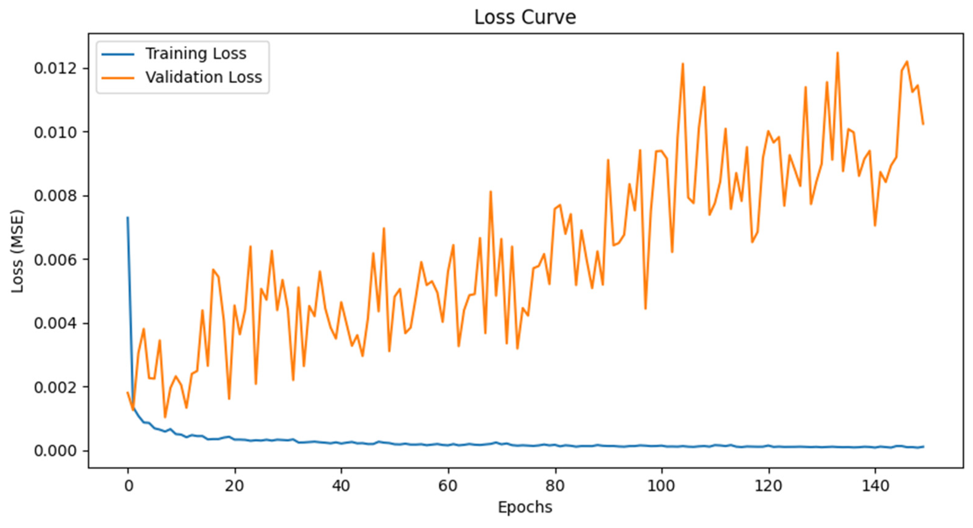
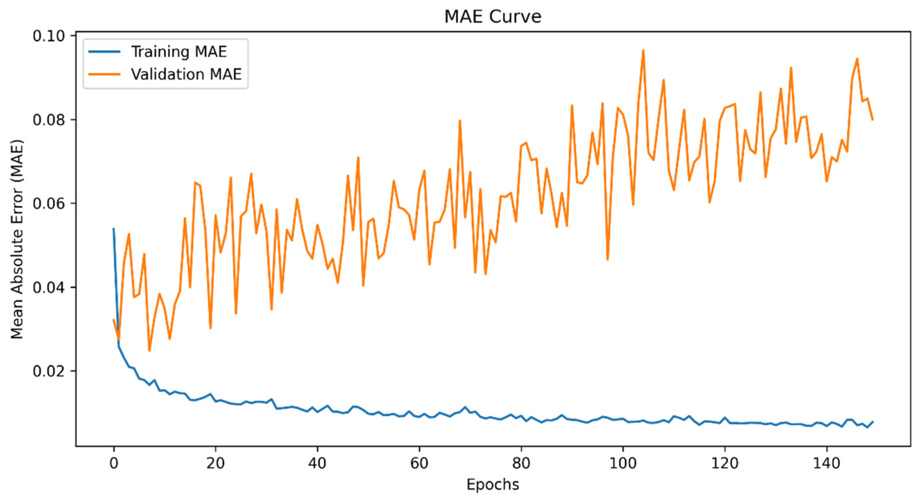
- Cross-Validation: Cross-validation is incorporated within the training phase to prevent overfitting and enhance model robustness (Sangeetha & Alfia, 2024). Training the model on multiple data folds allows for a more comprehensive performance assessment, ensuring that predictions remain reliable across different market conditions (Najem et al., 2024). This technique is particularly valuable in financial forecasting, where high variability and complex patterns are presented in historical data (Hoseinzade & Haratizadeh, 2019). To optimize the performance of the hybrid LSTM-CNN model, we conducted systematic hyperparameter tuning using grid search and empirical validation across multiple configurations. The final selection was based on achieving the lowest validation loss and highest predictive accuracy while mitigating overfitting risks. The number of epochs was set to 150, as loss stabilization was observed beyond 100 epochs, with overfitting emerging after 150. The batch size of 64 was selected after testing values of 32, 64, and 128; smaller batches resulted in unstable gradients, while larger batches slowed convergence. A learning rate of 0.001 was chosen for the Adam optimizer, as lower values (0.0001) led to prolonged convergence, while higher values (0.01) caused erratic training behaviour. To prevent overfitting, a dropout rate of 20% (0.2) was applied to the LSTM layer, ensuring a balance between model flexibility and generalization. Additionally, a lookback window of 30 days was used to capture historical patterns, aligning with financial literature that suggests this period provides an optimal trade-off between short-term noise and meaningful trend extraction.
- c-
- Evaluation Metrics: To assess the predictive performance of the hybrid LSTM-CNN model, we employ multiple quantitative metrics widely used in stock market forecasting (Najem et al., 2024). These metrics provide a holistic evaluation of both error minimization and model explanatory power. Root Mean Squared Error (RMSE) and Mean Absolute Error (MAE) serve as primary measures of prediction accuracy, ensuring precise error evaluation (Najem et al., 2024), while the R2 score assesses how well the model explains stock price variations (Hoseinzade & Haratizadeh, 2019). The Mean Absolute Percentage Error (MAPE) is included to measure relative prediction errors, which is particularly useful for stock prices that fluctuate across different price levels (Sangeetha & Alfia, 2024). Although financial performance metrics such as the Sharpe Ratio and Max Drawdown are commonly used in portfolio risk assessment, our study focuses primarily on price prediction rather than trading strategies. As a result, these metrics were not included in our evaluation framework, aligning with prior studies emphasizing RMSE, MAE, and R2 in financial time series forecasting (Hoseinzade & Haratizadeh, 2019).
3.4. Baseline Models for Comparison
3.5. Baseline Models for Comparison: Model Specifications
- (a)
- Support Vector Machines (SVMs)
- Weight vector;
- : Bias term;
- : Regularization parameter controlling margin width;
- : Slack variables to allow some misclassification;
- : Actual class label (1 or -1 for binary classification).
- (b)
- Random Forest (RF)
- : Number of trees in the forest;
- : Prediction from the tree based on input ;
- : Input features (e.g., historical prices, technical indicators).
- (c)
- Autoregressive Integrated Moving Averages (ARIMAs)
- : Stock price at time ;
- : Constant term;
- : AR coefficients for lag ;
- : MA coefficients for lag ;
- : White noise error term.
3.6. Model Architecture: LSTM-CNN Hybrid Model Specifications
- (a)
- Long Short-Term Memory (LSTM) Layer
- : Input features (e.g., stock price and technical indicators) at time t;
- : Hidden state at time t;
- : Cell state at time t;
- : Weight matrices for respective gates;
- , ,: Bias terms for respective gates;
- : Sigmoid activation function.
- (b)
- Convolutional Neural Network (CNN) Layer
- : Weight matrix of the filter;
- : Bias for the filter;
- * Convolution operator;
- : Output feature map;
- : Activation function (e.g., ReLU).
- (c)
- Model Fusion and Prediction Layer
- : Final predicted stock price;
- : Final hidden state from the LSTM;
- : Output from the CNN layer;
- : Weight matrix for the fully connected layer;
- : Bias term;
- : Activation function (e.g., linear or ReLU).
4. Results and Discussions
4.1. Model Performance Analysis
4.2. Key Adjustments and Model Improvements
- (a)
- Increasing Training Epochs from 100 to 150. A longer training period allowed the model to better capture long-term dependencies in stock price trends. However, further increases beyond 150 epochs yielded diminishing returns, as the model approached its learning capacity. Alternative configurations (100, 200 epochs; batch sizes of 32 and 128) were tested, but the selected settings provided the best trade-off between convergence and generalization.
- (b)
- Adjusting Batch Size from 32 to 64. Using a larger batch size helped smooth gradient updates, improving convergence stability, particularly in periods of high market volatility.
4.3. Model Evaluation and Comparative Analysis
5. Conclusions and Recommendations
Funding
Institutional Review Board Statement
Informed Consent Statement
Data Availability Statement
Conflicts of Interest
| 1 | Equation (1) aligns with the approach used by Zanc et al. (2019) to optimize binary classification tasks, focusing on maximizing margin separation in high-dimensional datasets. |
| 2 | |
| 3 | Although ARIMA lacks the complexity of ML-based models, its inclusion as a baseline highlights the relative benefits of deep learning techniques for long-term forecasts (Shah et al., 2019). |
| 4 | The forget gate selectively removes irrelevant information from previous sequences, a critical mechanism in time series forecasting. As Najem et al. (2024) emphasized, this ensures that only historically significant data influences predictions. |
| 5 | The updated cell state integrates prior information with new input, allowing the LSTM to capture patterns spanning extended periods, making it ideal for financial time series forecasting (Shah et al., 2019). |
| 6 | CNNs apply convolutional filters to capture localized trends in technical indicators. This aligns with findings by Hoseinzade and Haratizadeh (2019), who demonstrated that CNNs effectively detect chart patterns like peaks and troughs. |
| 7 | The fusion of LSTM and CNN outputs into a fully connected layer synthesizes temporal and spatial insights, a technique validated by Sangeetha and Alfia (2024) in their comparative studies of hybrid architectures. |
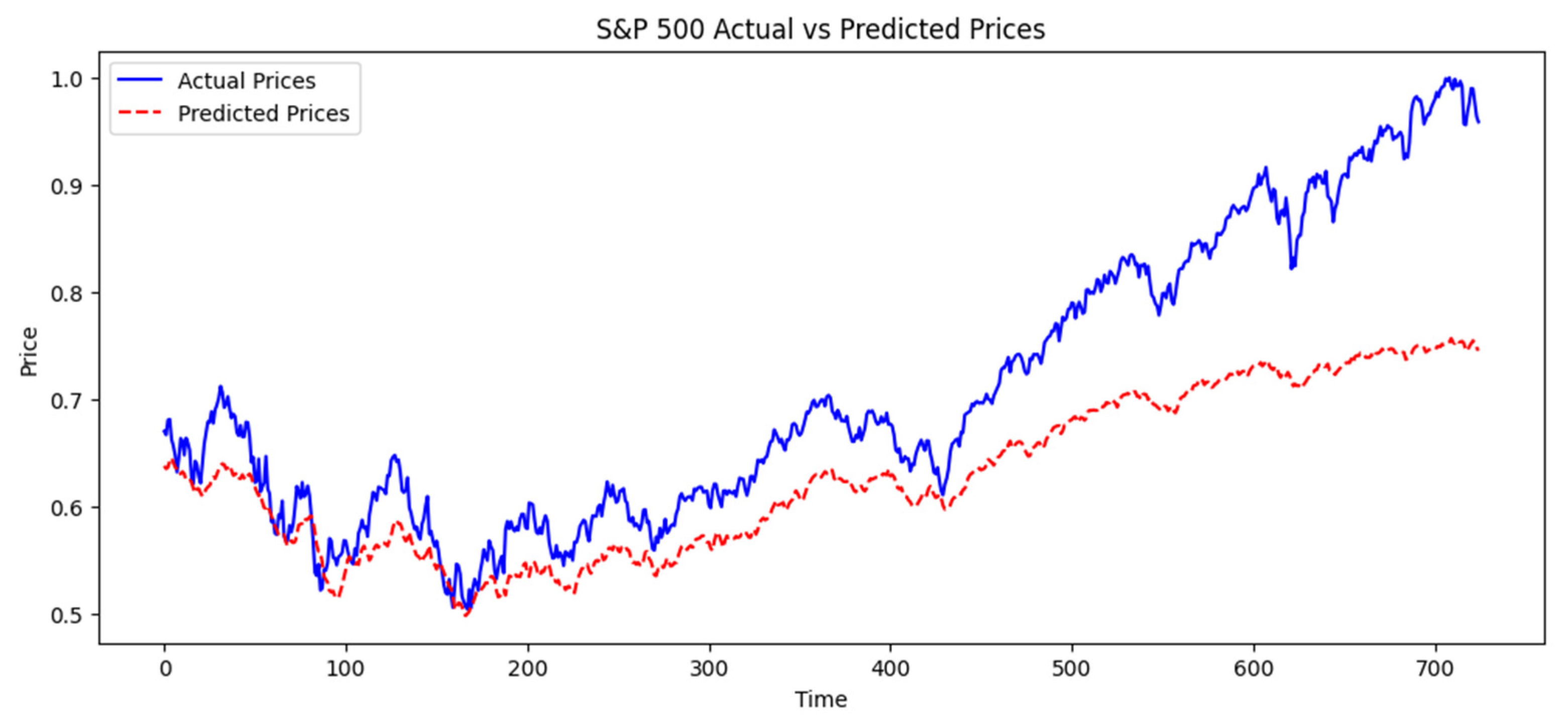
| 8 | Figure 3 presents a representative subset of the testing period, covering approximately 720 trading days (~3 years) rather than the full 5-year test period (2020–2024). This selection was made to enhance visualization clarity and highlight key trends. The complete test dataset includes stock price movements for the entire 2020–2024 period, ensuring that all relevant market conditions, including volatility and macroeconomic events, are accounted for in the analysis. |
| 9 | One key limitation of our training setup is that the dataset used for model training (2010–2019) does not include extreme market disruptions such as the COVID-19 pandemic. As observed in Figure 3, the model performed well in stable market conditions but deviated significantly during the latter part of the testing period, which coincides with high volatility events post-2020. This suggests that the absence of crisis-period data in training may have impacted the model’s ability to generalize to extreme market conditions. Future research could address this limitation by incorporating transfer learning, where a pre-trained model is fine-tuned on crisis-period data to enhance adaptability. Additionally, online learning techniques could be implemented to allow real-time model updates as new market conditions emerge, ensuring continuous adaptation to unexpected shocks such as financial crises or global pandemics. |
| 10 | While our study focuses on demonstrating the advantages of hybrid deep learning over traditional models, future research could explore alternative hybrid architectures to refine predictive performance. Potential candidates include an LSTM-GRU hybrid, which integrates two recurrent units to optimize sequential pattern recognition, or CNN-GRU models, which may provide an alternative fusion of spatial and temporal dependencies. Additionally, Transformer-based architectures have shown promise in financial forecasting due to their attention mechanisms, allowing for enhanced adaptability to market fluctuations. Investigating these alternatives would provide deeper insights into the optimal architectures for stock market prediction and risk management strategies. |
References
- AI, L., School, T. N., Ji, S., Song, Z., Zhong, F., Jia, J., Wu, Z., Cao, Z., & Tianhao, X. (2025). Chinese stock prediction based on a multi-modal transformer framework: Macro-micro information fusion. arXiv, arXiv:2501.16621. [Google Scholar]
- Atsalakis, G. S., & Valavanis, K. P. (2009). Surveying stock market forecasting techniques—Part II: Soft computing methods. Expert Systems with Applications, 36(3), 5932–5941. [Google Scholar] [CrossRef]
- Badr, H., Wanas, N., & Fayek, M. (2024). Unsupervised domain adaptation via weighted sequential discriminative feature learning for sentiment analysis. Applied Sciences, 14(1), 406. [Google Scholar] [CrossRef]
- Bao, W., Yue, J., & Rao, Y. (2017). A deep learning framework for financial time series using stacked autoencoders and long-short term memory. PLoS ONE, 12(7), e0180944. [Google Scholar] [CrossRef] [PubMed]
- Fischer, T., & Krauss, C. (2018). Deep learning with long short-term memory networks for financial market predictions. European Journal of Operational Research, 270(2), 654–669. [Google Scholar] [CrossRef]
- Hao, J., He, F., Ma, F., & Zhang, X. (2023). Machine learning vs deep learning in stock market investment: An international evidence. Annals of Operations Research. [Google Scholar] [CrossRef]
- Hoseinzade, E., & Haratizadeh, S. (2019). CNNpred: CNN-based stock market prediction using a diverse set of variables. Expert Systems with Applications, 129, 273–285. [Google Scholar] [CrossRef]
- Hossain, M. A., Karim, R., Thulasiram, R., Bruce, N. D. B., & Wang, Y. (2018, November 18–21). Hybrid deep learning model for stock price prediction. 2018 IEEE Symposium Series on Computational Intelligence (SSCI) (pp. 1837–1844), Bangalore, India. [Google Scholar] [CrossRef]
- Huck, N. (2019). Large data sets and machine learning: Applications to statistical arbitrage. European Journal of Operational Research, 278(1), 330–348. [Google Scholar] [CrossRef]
- Kaur, A., Joshi, M., Singh, G., & Sharma, S. (2024). The impact of corporate reputation on cost of debt: A panel data analysis of Indian listed firms. Journal of Risk and Financial Management, 17(8), 367. [Google Scholar] [CrossRef]
- Kwon, D. (2025). Oil shocks, US uncertainty, and emerging corporate bond markets. Journal of Risk and Financial Management, 18(1), 25. [Google Scholar] [CrossRef]
- LeCun, Y., Bengio, Y., & Hinton, G. (2015). Deep learning. Nature, 521(7553), 436–444. [Google Scholar] [CrossRef] [PubMed]
- Leippold, M., Wang, Q., & Zhou, W. (2022). Machine learning in the Chinese stock market. Journal of Financial Economics, 145(1), 64–82. [Google Scholar]
- Long, W., Lu, Z., & Cui, L. (2019). Deep learning-based feature engineering for stock price movement prediction. Knowledge-Based Systems, 164, 163–173. [Google Scholar] [CrossRef]
- Najem, R., Bahnasse, A., & Talea, M. (2024). Toward an enhanced stock market forecasting with machine learning and deep learning models. Procedia Computer Science, 241, 97–103. [Google Scholar]
- Nelson, D. M., Pereira, A. C., & De Oliveira, R. A. (2017, May 14–19). Stock market’s price movement prediction with LSTM neural networks. 2017 International Joint Conference on Neural Networks (IJCNN) (pp. 1419–1426), Anchorage, AK, USA. [Google Scholar] [CrossRef]
- Sangeetha, J. M., & Alfia, K. J. (2024). Financial stock market forecast using evaluated linear regression-based machine learning technique. Measurement: Sensors, 31, 100950. [Google Scholar]
- Shah, D., Isah, H., & Zulkernine, F. (2019). Stock market analysis: A review and taxonomy of prediction techniques. International Journal of Financial Studies, 7(2), 26. [Google Scholar] [CrossRef]
- Sharma, R., & Mehta, K. (Eds.). (2024). Deep learning tools for predicting stock market movements. John Wiley & Sons. [Google Scholar]
- Singh, R. K., Singh, Y., Kumar, S., Kumar, A., & Alruwaili, W. S. (2024). Mapping risk–return linkages and volatility spillover in BRICS stock markets through the lens of linear and non-linear GARCH models. Journal of Risk and Financial Management, 17(10), 437. [Google Scholar] [CrossRef]
- Zanc, R., Cioara, T., & Anghel, I. (2019, September 5–7). Forecasting financial markets using deep learning. 2019 IEEE 15th International Conference on Intelligent Computer Communication and Processing (ICCP) (pp. 459–466), Cluj-Napoca, Romania. [Google Scholar]

| SVMs | RF | ARIMAs | |
|---|---|---|---|
| Purpose | SVMs is a classification model widely used in financial forecasting for its ability to analyze the relationship between input features (such as historical stock prices and technical indicators) and stock price movements. | Random Forest is an ensemble model combining multiple decision trees to improve prediction stability and accuracy, particularly for regression task stock price forecasting. | ARIMAs is a traditional time series forecasting model extensively applied in financial data analysis. It is instrumental in identifying patterns within historical data and projecting future price trends. |
| Application | This study uses SVMs as a binary classifier to predict the direction of stock price changes (e.g., price increase or decrease) rather than specific price values. | In this context, RF is used as a regression model to predict stock prices based on historical price data and technical indicators. It leverages the aggregated outputs from multiple decision trees to yield stable predictions. | ARIMAs generate forecasts based solely on historical stock price data as a benchmark model without incorporating additional technical indicators. This allows for a direct comparison between the predictive accuracy of traditional statistical methods and more complex machine learning models. |
| Strengths | SVMs effectively distinguishes between categories (e.g., upward or downward price movement), particularly in complex, high-dimensional data cases. Its strength lies in maximizing the margin between categories, which helps to enhance generalization and reduce the risk of overfitting. | The RF model is known for its robustness in handling high-dimensional datasets and reducing the variance of individual decision trees. It provides reliable results in stock forecasting due to its ability to mitigate the effects of outliers and noisy data, making it a suitable benchmark for evaluating the performance of the hybrid model. | ARIMAs is well-regarded for its simplicity and interpretability in financial forecasting. While it cannot capture non-linear dependencies and interactions, it remains a reliable baseline to gauge the added value provided by advanced hybrid models. |
| Metric | Value |
|---|---|
| RMSE | 0.1012 |
| MAE | 0.08 |
| R2 Score | 0.4199 |
| MAPE | 10.22% |
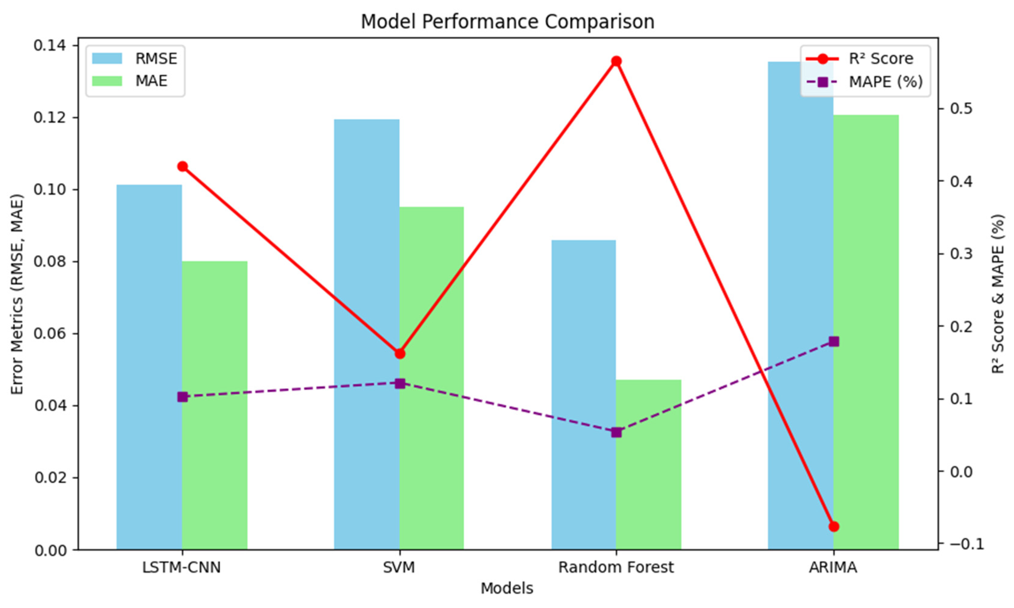
| Model | RMSE | MAE | R2 Score | MAPE | 95% CI (RMSE) | 95% CI (MAE) | 95% CI (R2) | p-Value |
|---|---|---|---|---|---|---|---|---|
| LSTM-CNN (Hybrid Model) | 0.1012 | 0.08 | 0.4199 | 10.22% | (0.0992, 0.1031) | (0.0791, 0.0815) | (0.4121, 0.4278) | <0.05 |
| SVMs | 0.1194 | 0.095 | 0.1617 | 12.14% | (0.1173, 0.1218) | (0.0934, 0.0969) | (0.1561, 0.1689) | <0.05 |
| Random Forest | 0.0859 | 0.0471 | 0.5655 | 5.42% | (0.0847, 0.0872) | (0.0461, 0.0480) | (0.5567, 0.5741) | <0.05 |
| ARIMAs | 0.1353 | 0.1206 | −0.0764 | 17.81% | (0.1332, 0.1379) | (0.1185, 0.1231) | (−0.0821, −0.0694) | <0.05 |
Disclaimer/Publisher’s Note: The statements, opinions and data contained in all publications are solely those of the individual author(s) and contributor(s) and not of MDPI and/or the editor(s). MDPI and/or the editor(s) disclaim responsibility for any injury to people or property resulting from any ideas, methods, instructions or products referred to in the content. |
© 2025 by the author. Licensee MDPI, Basel, Switzerland. This article is an open access article distributed under the terms and conditions of the Creative Commons Attribution (CC BY) license (https://creativecommons.org/licenses/by/4.0/).
Share and Cite
Fozap, F.M.P. Hybrid Machine Learning Models for Long-Term Stock Market Forecasting: Integrating Technical Indicators. J. Risk Financial Manag. 2025, 18, 201. https://doi.org/10.3390/jrfm18040201
Fozap FMP. Hybrid Machine Learning Models for Long-Term Stock Market Forecasting: Integrating Technical Indicators. Journal of Risk and Financial Management. 2025; 18(4):201. https://doi.org/10.3390/jrfm18040201
Chicago/Turabian StyleFozap, Francis Magloire Peujio. 2025. "Hybrid Machine Learning Models for Long-Term Stock Market Forecasting: Integrating Technical Indicators" Journal of Risk and Financial Management 18, no. 4: 201. https://doi.org/10.3390/jrfm18040201
APA StyleFozap, F. M. P. (2025). Hybrid Machine Learning Models for Long-Term Stock Market Forecasting: Integrating Technical Indicators. Journal of Risk and Financial Management, 18(4), 201. https://doi.org/10.3390/jrfm18040201