Article

Persisting Stickiness in Backwardation Among Major Agricultural Commodities

by
Peter Cincinelli
1,*,
Ameeta Jaiswal-Dale
2 and
Giovanna Zanotti
1
1
Department of Management, University of Bergamo, Via dei Caniana 2, 24129 Bergamo, Italy
2
Department of Finance, Opus College of Business, Terrance Murphy Hall, University of St. Thomas, Minneapolis, MN 55403, USA
*
Author to whom correspondence should be addressed.
J. Risk Financial Manag. 2025, 18(12), 674; https://doi.org/10.3390/jrfm18120674 (registering DOI)
Submission received: 2 October 2025 / Revised: 10 November 2025 / Accepted: 11 November 2025 / Published: 27 November 2025
(This article belongs to the Section Financial Markets)

Abstract

In this paper, we investigate the relationship between spot and futures contracts in the context of spot prices being higher than futures (backwardation). We focus on the persistence in stickiness during backwardation periods by covering major agricultural commodities (corn, oats, soybeans, soybean oil, wheat, and hard red wheat). The period of investigation, January 2000–August 2022, comprises many subperiods, including the pre-2008 global financial crisis, the global financial crisis, the single event of 2014, and the post-2014 stability and growth in world trade. We find the presence of price backwardation and its stickiness for corn and wheat, with the most significant determinants being convenience yield and interest risk.

1. Introduction

Price discovery remains the driver for price movements in all market activities. It is taking on increasing importance in commodities partly due to their increasing financialization as an independent asset class. The study of financialization has steadily gathered momentum starting from the 1980s (Fama & French, 1987) and earlier, fueled by the Black & Scholes options pricing process and the need to feed and shelter the world’s growing population in the context of increasing challenges, both environmental and political. Today, we also see another aspect of financialization with the demand of commodities as collateral (Jo et al., 2022).
In this paper, intrigued by this aspect of increases in the financialization of commodities, we extend this initial analysis to further examine how the price discovery varies between spot and futures contract. We focus on the relationship between spot and futures contract in the context of futures prices being higher than spot contango and when backwardation is not the case. The research question is tackled in the following steps. First, we identify the periods of backwardation in agricultural commodities, the when. Second, we then proceed to identify the variables that are the determinants of this backwardation and the cause of price stickiness during the backwardation, the how. Third, using a probit model we test for the probability of this price stickiness during backwardation, explaining the why.
The persistence in stickiness during backwardation periods is evaluated in our chosen agricultural commodities (corn, oats, soybeans, soybean oil, wheat, and hard red wheat). We cover the major agricultural commodities experiencing global price volatility, yet are essential for civil society security and in constant increasing demand—wheat, corn, soybeans and oats. This paper examines price stickiness during periods of backwardation for wheat, corn, soybeans and oats. The period of investigation January 2000–August 2022 comprises many subperiods, such as the pre-2008 global financial crisis, the global financial crisis (GFC), the single event of 2014, and the post 2014 stability and growth in world trade.
The concept of stickiness, observed in backwardation within agricultural commodities, is related to the prolonged persistence of this market structure. This situation indicates a resistance to shifting back into contango, where future prices are higher than spot prices. Such dynamics may reflect underlying supply–demand imbalances and market expectations, contributing to the enduring state of backwardation. Investigating the stickiness of backwardation is important for the following reasons. First, a prolonged period of backwardation indicates market imbalances, reflecting either strong spot demand or concerns regarding the future supply. Second, from a risk management perspective, the tendency for backwardation to persist allows market participants to develop more reliable hedging and arbitrage strategies. Third, the presence of sticky backwardation emphasizes the role of market participants. If backwardation does not revert quickly, it indicates that beliefs about scarcity or abundance remain stable over time, which may lead to significant implications for portfolio allocation and risk assessment.
Based on the spot–future relationship, to avoid arbitrage opportunities, spot and futures prices should move together across time (Hull, 2003). Spot and future prices are closely related because they are driven by the same underlying information. However, the nature of this relationship should also depend on different factors, such as whether a commodity is storable of non-storable market expectations and seasonal effects. The extant literature limits the analysis on the long-run equilibrium relationship between commodity spot and futures prices (Garcia & Leuthold, 2004; Giot, 2003; Hakkio & Rush, 1989; Hernandez & Torero, 2010; Martin & Garcia, 1981; Wahab & Lashgari, 1993). However, only a few investigate the time dynamic of such a relationship, i.e., a potential structural break exists in the cointegration vector (Dawson et al., 2006; Maslyuk & Smyth, 2009).
Our results are summarized as follows. First, we find robust results for the investigation of our hypothesis. We identify the presence of price backwardation, and its stickiness for corn and wheat is expected. These are commodities with a global market, sensitive to the volatilities of supply and demand, but most importantly responding to corporate procurement. Commodity futures give companies insurance for the future value of their outputs. Second, the interesting fact, beyond the presence of backwardation, was its intensity (as shown by the β 3 ). This led us to proceed with confidence to stage two, to investigate the determinants of stickiness in prices during backwardation. The most significant determinants are convenience yield and interest risk. This is in line with G. B. Gorton et al. (2013) and Jo et al. (2022).
Our paper contributes to the literature in several ways. First, besides the works of Fama and French (1987) and Jo et al. (2022), we extend the work done by G. Gorton and Rouwenhorst (2006) and G. B. Gorton et al. (2013) on financialization of agricultural commodities using convenience yield, state of inventories and commodity futures risk premium. Our work is influenced by the Jo et al. (2022) as they examine the role of open interest. Second, our value added is in extending this reasoning over a longer period of time but more importantly, identifying the time frame, the when of the occurrence.
The remainder of this paper is organized as follows. Section 2 presents the literature review. Section 3 shows the stylized facts on commodity spot and future prices. Section 4 presents the empirical results, while Section 5 provides sensitivity analysis. Section 6 concludes.

2. Literature Review

The literature exploring the interactions between spot and futures prices in commodity markets is extensive. Several studies report that future markets are efficient, while other contributions contradict futures price prediction interpretation (Bopp & Lady, 1991; Moosa & Al-Loughani, 1994; Serletis, 1991). Over the past 40 years, financial explanations of agricultural price patterns gained support, especially during the price boom of 2005–2008 (Awokuse, 2005; Bordo, 1980; Chambers & Just, 1982; Cooper et al., 1975; Taylor, 1995), and during booms in equity and real estate prices (Gilbert, 2010).
Recently, the financialization of commodity futures and spot markets has provoked a debate regarding its implications for policy and the efficiency of commodity pricing. Economists and policymakers contend that the extreme fluctuations in global food prices, observed during the 2007–2008 period, were influenced by speculative activities within the global commodity market, leading to the creation of bubbles that inflated futures prices beyond fundamental values. Conversely, some researchers express skepticism about characterizing this period as a bubble, arguing instead that fundamental supply and demand dynamics were the predominant drivers. Factors such as the rising consumption of biofuels, the burgeoning demand from emerging economies like China and India, the crash of stock prices, the escalating oil prices, and the depreciation of the dollar are cited as critical influences shaping market conditions during that time (Irwin et al., 2011).
Some authors argue that other factors intervened in the commodity prices movement during the global financial crisis. Masters (2008) and Robles and Cooke (2009) find that the surge in prices, caused by speculation, may increase poverty. Ghosh (2010) reports that the financial crises increase food insecurity by imposing constraints on fiscal policies and food imports in developing countries. Gilbert (2010) studies the drivers of the recent increase in food prices. He concludes that the demand for grains and oil seeds is the main cause of the price rise. Tang and Xiong (2010) identify a link between futures price movements and commodity index investment, suggesting that the rise of index investors in commodities has led to financialization in these markets, resulting in increased correlation between commodity prices and financial assets. Cincinelli et al. (2021) investigate the cross-market price linkages in actively traded, major agricultural and energy commodities. They find a negative relationship among all the agricultural commodities during the commodity depression and an increase in the energy prices, confirming the relationship between the stock and crude oil markets due to the financialization of commodities.
There are also some contributions that demonstrate that the fluctuations in commodity prices are mainly driven by market supply and demand. In particular, Headey and Fan (2008) argue that while futures markets may have worsened agricultural price volatility, they are not a primary cause of the overall price surge. Instead, they suggest that the rise in biofuel production explains increasing corn and soybean prices, along with other factors such as rising oil prices and the depreciation of the US dollar. Other studies examine the rise in index fund investment over the last decade, reporting minimal linkage between commodity prices and index fund market positions (Irwin & Sanders, 2011; Sanders & Irwin, 2010; Stoll & Whaley, 2010).
A market has a price discovery function when it rapidly reflects new information. Price discovery is a critical issue regarding the impact of financial instruments on food commodity prices. While derivatives are known to provide benefits, such as information dissemination and efficient resource allocation, there is a general consensus that they may lead to excessive speculation, distorting prices away from their fundamental values and destabilizing real markets (Fleming & Ostdiek, 1999; Gerety & Mulherin, 1991).
Spot prices are typically determined in future markets. The same fundamental factors influence the spot and futures prices for the same commodity. They may change when new information is available, prompting market participants to adjust their physical supply and demand assessments. Since futures contracts usually do not necessitate the delivery of the commodity and can be executed with minimal upfront cash, futures markets tend to respond more swiftly than spot markets (Silvapulle & Moosa, 1999). Garbade and Silber (1983) and Yang et al. (2001), by investigating the price discovery for corn and soybeans, find that futures markets play a predominant role over spot markets in the registration and dissemination of information. Crain and Lee (1996) report that wheat futures price markets dominate spot markets in the price discovery process changes. Hernandez and Torero (2010), analyzing spot and futures prices for wheat, corn, and soybeans, show that future prices Granger-cause spot prices for corn and wheat, and that the causal relationship is stronger than in the past. A possible explanation is related to the importance of electronic trading of futures contracts. However, other studies present different results, showing that spot prices dominate futures prices (Kuiper et al., 2002; Mohan & Love, 2004; Quan, 1992). Finally, Baldi et al. (2011) detect breaks in the food commodity markets, which are related to events that significantly affected the supply and demand for corn and soybeans used for food and energy purposes. Dimpfl et al. (2017) find evidence that the prices of corn, wheat, soybeans, soybean meal and oil, feeder and live cattle, and lean hogs are almost uniquely formed in the spot market.

3. Stylized Facts on Commodity Spot and Future Prices

We collect data from BarChart, a provider of market data and services to the financial and commodity industries. The following panel of figures reports the trend of the spot and future monthly prices for the agricultural grain commodities sector, such as corn, oats, soybeans, soybean oil, wheat, and hard red wheat1. According to BarChart2, we provide the specification for each commodity: Corn: The largest futures market for corn is at the CME Group. However, corn futures also trade at the B3 exchange, the Dalian Commodity Exchange, the Euronext Derivatives Market, the JSE Securities Exchange, the MATba ROFEX exchange, and the Osaka Exchange. The CME futures contract calls for delivering 5000 bushels of n. 2 yellow corn at par contract price, n. 1 yellow at 1–1/2 cents per bushel over the contract price, or n. 3 yellow at 1–1/2 cents per bushel below the contract price. Oats: The largest futures market for oats is the Chicago Board of Trade (CBOT), part of the CME Group. The contract covers 5000 bushels of n. 2 heavy oats. Soybeans: The primary market for soybean futures is at the CME Group. The CME’s soybean contract calls for delivering 5000 bushels of n. 2 yellow soybeans (at contract par), n. 1 yellow soybeans (at 6 cents per bushel above the contract price), or n. 3 yellow soybeans (at 6 cents under the contract price). Soybean futures are also traded at Brazil, Argentina, China, and Tokyo exchanges. Soybean oil is the natural oil extracted from whole soybeans. The largest futures market for soybean oil is the CBOT. Wheat and Hard Red Wheat: They are traded at the CME Group, ICE Futures US Exchange, the MatbaRofex exchange (Argentina), Sydney Futures Exchange (SFE), Euronext (Paris), Zhengzhou Commodity Exchange, and the South Africa Futures Exchange. The CME’s wheat futures contract calls for the delivery of soft red wheat (n. 1 and 2), hard red winter wheat (n. 1 and 2), dark northern spring wheat (n. 1 and 2), n.1 northern spring at 3 cents/bushel premium, or n. 2 northern spring at par (source: BarChart).
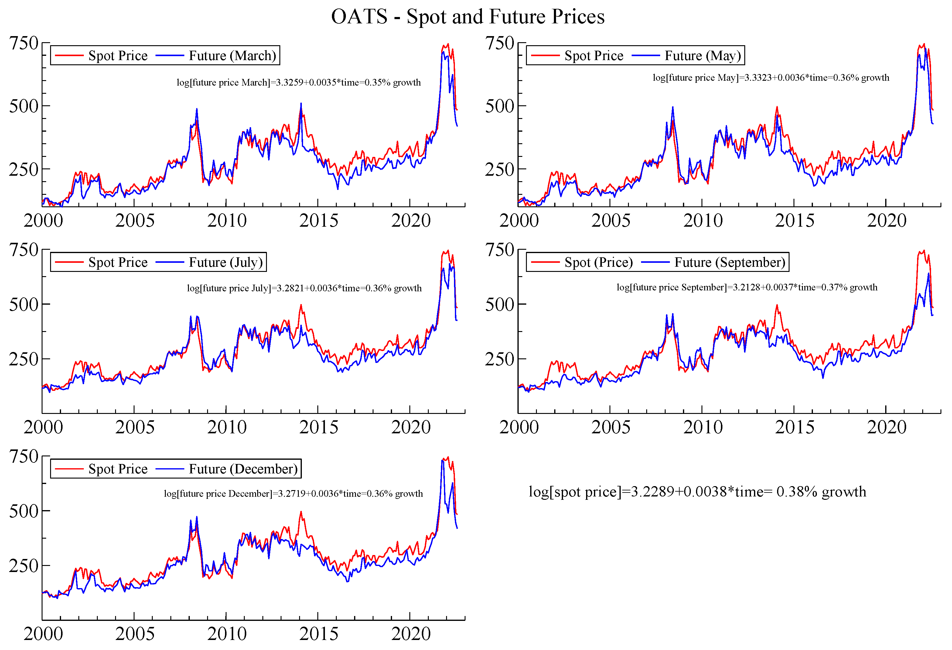
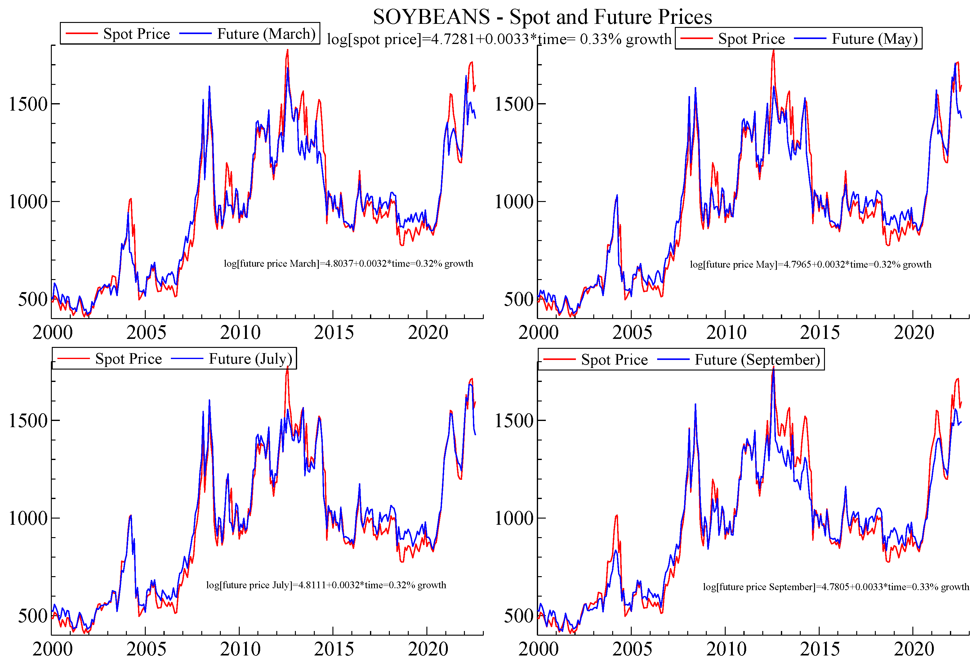
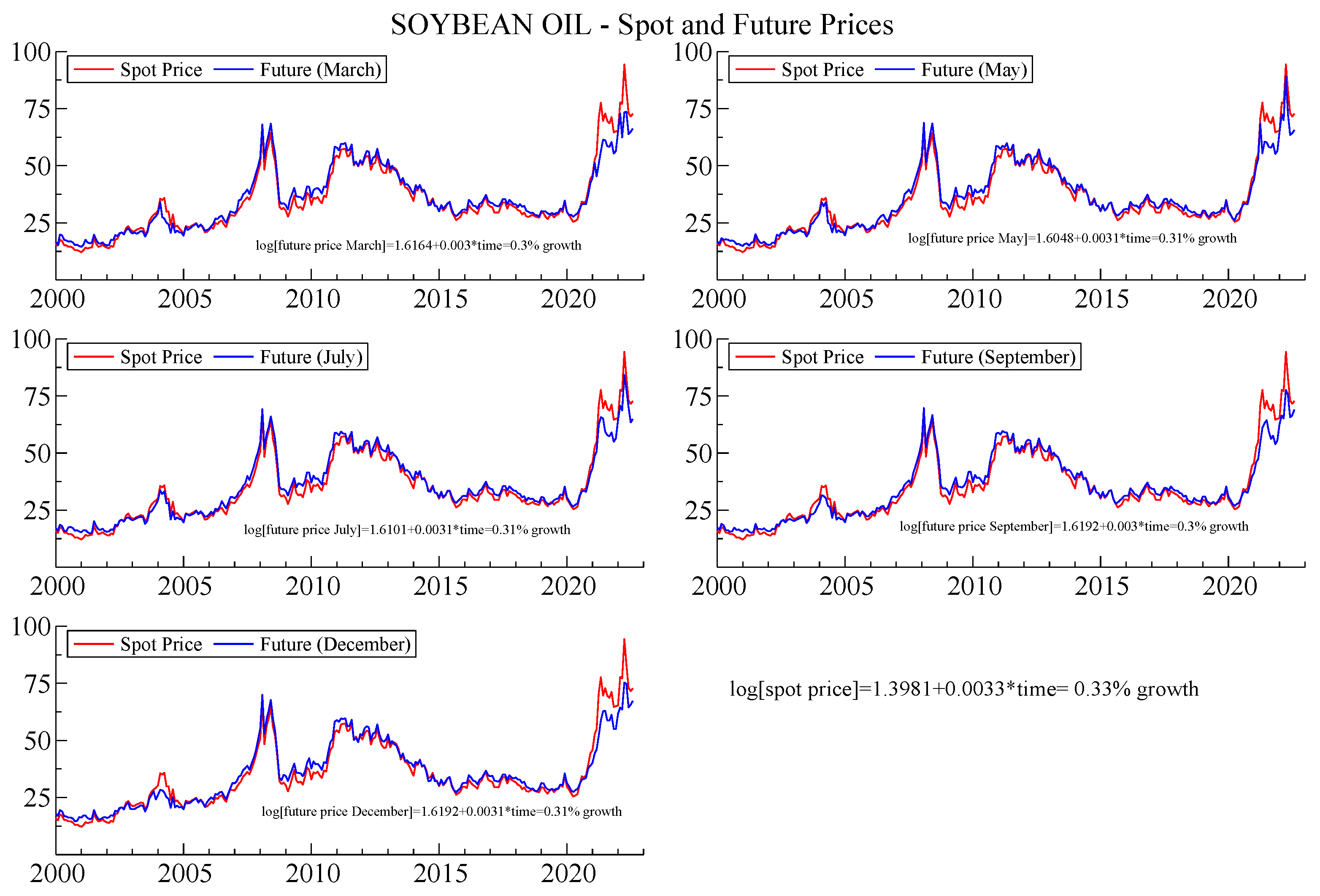
Fiure 1, Fiure 2, Fiure 3, Fiure 4, Fiure 5 and Fiure 6 illustrate the main stylized facts concerning commodity spot and future prices for corn, oats, soybeans, soybean oil, wheat and hard red wheat.
After 2001, commodity prices began to rise slowly and reached levels similar to those of the mid-1980s by 2004. In early 2006, prices in the commodity grain sector started to increase more rapidly. Over the following ten years, these prices surged to new highs. However, starting in 2013, they experienced a dramatic decline due to the effects of the subprime financial crisis and the sovereign debt crisis. Generally, the price trends indicate that they tend to rise and then recede in a similar pattern. This recurring trend may occur because buyers can switch to cheaper substitutes among these commodities. Each period of rapidly rising prices has typically been followed by a retreat back to pre-spike levels.
The conflict in Ukraine hurt the agricultural commodity market, leading to a significant increase in the prices of the principal agricultural commodities. Starting in July 2022, agricultural commodity prices returned to pre-conflict levels, mainly due to increasing fears of a recession. The rise in interest rates dampened the demand in the real estate sector, resulting in a decreased consumption of construction materials like copper and lumber. Consumer spending on discretionary items such as apparel, appliances, and automobiles decreased the demand for several materials, including aluminum and zinc. In addition, some of the supply constraints that previously fueled price increases have started to ease due to favorable weather conditions in grain-producing regions.

4. Empirical Analysis

In this section, we present the empirical analysis regarding how stickiness during backwardation periods is measured (Section 4.1), and the determinants of stickiness (Section 4.2).

4.1. Measuring Stickiness in Backwardation

We derive the relationship between spot and futures prices from the spot–future parity, which implies that spot and futures prices should move together across time to avoid constant arbitrage opportunities based on the spot–futures relationship (Hull, 2003):
F 0 = S 0 e ( r + u ) T
F 0 e y T = S 0 e ( r + u ) T
F 0 = S 0 e ( r + u y ) T
The presence of stickiness between spot price and future contract price, during backwardation periods, will be investigated as follows:
log S p o t P r i c e s t = β 0 + β 1 log F u t u r e P r i c e s t 2 + + β 2 B a c k w a r d a t i o n D u m m y t + + β 3 B a c k w a r d a t i o n D u m m y t log F u t u r e P r i c e s t 2 + + β 4 X t 2 + ε i , t
where Spot Pricesi,t represents monthly commodities spot prices; Future Pricesi,t−2 represents monthly commodities future contract prices; Backwardation Dummy takes the value of 1 when spot prices are greater than future prices, between t 1 and t, and 0 otherwise. X t 2 is a vector of explanatory variables such as the following: V I X t 2 is the Chicago Board Options Exchange’s (CBOE) Volatility Index, a measure of the stock market’s expectation of volatility based on S&P 500 index options; C P I t 2 is the monthly US Consumer Price Index ratio; and T B i l l t 1 is the 3-month US treasury bill. The transition of the futures curve from a state of contango to a prolonged period of backwardation signals a market environment where physical traders anticipate price declines. If this backwardation is persistent, it indicates that traders are continuously hedging against their positions due to expectations of falling prices. Consequently, the enduring nature of backwardation, referred to as “sticky backwardation”, suggests an increasingly high probability that market prices will indeed decline. This behavior reflects the conviction of informed physical traders, who are willing to stake capital on the expectation of a downturn on a daily basis. We thus expect β 3 > 0 .
We find evidence of persistence in stickiness during backwardation periods for some commodities. In particular, the stickiness is reported for only Corn commodity for March and December contracts (Table 1, Table 2 and Table 3). An increase of one standard deviation of Corn future contracts in March would lead to a 2.85 basis points increase in stickiness persistence monthly. An increase of one standard deviation of Corn future contracts in September would lead to a 3.73 basis points increase in stickiness persistence. Regarding Corn future contracts in December, an increase of one standard deviation would lead to a 3.34 basis points increase in stickiness persistence for each month. Regarding Hard Red Wheat, an increase of one standard deviation of future contracts in December would lead to a 4.91 basis points decrease in stickiness persistence monthly (Table 3). For the May and July contracts, we do not find any evidence of persistence stickiness during backwardation periods for any of the commodities (Table 4 and Table 5).

4.2. Determinants of Stickiness Backwardation

Once we identified the stickiness persistence in agricultural commodities, we investigate the determinants of such stickiness persistence in the US financial system using the following probit model:
P r ( Y t = 1 | X t 1 ) = Φ ( β X t 1 )
where Φ is the cumulative normal distribution function; Y t takes value 1 when a time series shows backwardation and 0 otherwise; X t 1 is a vector of weekly explanatory variables such as C o n v e n i e n c e Y i e l d t 1 defined as follows:
C o n v e n i e n c e Y i e l d = ln ( F ( t , T 1 ) ) ln ( F ( t , T 2 ) ) T 2 T 1 + γ t
where F ( t , T 1 ) and F ( t , T 2 ) are futures prices at month t with maturity T 1 and T 2 , respectively; γ t denotes the local interest rate Libor for US; I n t e r e s t   R a t e R i s k t 1 is the difference between 3-month Libor and overnight 3-month Libor for US; S & P 500 r e t u r n s t 1 is the monthly returns of S&P 500; B a l t i c D r y I n d e x C h a n g e t 1 is the monthly change in Baltic Dry index; and V I X t 2 is the Chicago Board Options Exchange’s (CBOE) Volatility Index, a measure of the stock market’s expectation of volatility based on S&P 500 index options.
According to Goswami et al. (2022), we also control for the Variable Storage Rate (VSR) and the Kraft squeeze. Specifically, for the VSR, we introduce a dummy variable that equals 1 during the period from July 2010 to August 2022 for wheat and from March 2018 to August 2022 for hard red wheat markets; otherwise, it equals 0. The VSR was introduced to address the issue of weak convergence between cash and futures prices, particularly following large harvests that led to an oversupply of wheat. This oversupply resulted in a shortage of storage space, which in turn increased storage costs and weakened the basis values for farmers. Meanwhile, for the Kraft squeeze for wheat markets, we use a dummy variable equal to 1 for March 2008 and December 2011, 0 otherwise.
Table 6, Table 7, Table 8, Table 9, Table 10 and Table 11, report the results. We find that a rise in convenience yields, for each monthly future contract, is associated with a higher probability of a price spike during this period, thus a lower price backwardation and its stickiness. A possible explanation is that warehouse operators, by acquiring the commodity in the spot markets with less urgency, reduce the pressure of backwardation. This is in line with the theory of storage (Brennan, 1958; Telser, 1958; Triantafyllou et al., 2020; Working, 1948), as the forward spread represents the marginal convenience yield of holding physical inventory.
In addition, the 2007 transition from warehouse receipts to shipping certificates represented a significant evolution in logistics and cost management within the supply chain. Previously, the reliance on physical warehouse receipts imposed immediate storage costs on buyers upon receipt of goods. The introduction of shipping certificates allowed certificate holders to defer load-out, thus incurring storage fees at a predetermined fixed rate. This model effectively decouples the immediate physical delivery requirement from the expiration of futures contracts, enhancing strategic flexibility in inventory management and optimizing cost control mechanisms.
Another explanation relates to the implementation of the Variable Storage Rate (VSR) mechanisms by the CME Group, started in July 2010 and fully operational by 2011 for CBOT corn, soybean, and wheat contracts, and that represented a strategic response to persistent non-convergence issues in the futures market. This mechanism enabled the adjustment of storage fees in accordance with futures spreads, thereby enhancing the alignment of delivery incentives with prevailing market conditions. The adoption of VSR was a direct reaction to historical non-convergence issues, including significant market squeezes like the March 2008 incident and the notorious Kraft squeeze of 2011, which highlighted critical deficiencies in the fixed storage rate contracts’ incentive structure. The coefficients for both VSR and the Kraft squeeze are positive without affecting the main results. Additionally, the change in July 2022 may be linked to the Black Sea Grain Initiative, which facilitated the resumption of Ukrainian grain exports through the Black Sea, further influencing market dynamics3.
Thus, according to our findings, when agricultural commodity producers and consumers hold low physical inventories (more negative forward spread), the probability of a price spike occurring is significantly increased. Our findings are in line with the more recent empirical findings of Bobenrieth et al. (2013) who find that agricultural stocks-to-use ratios, which are essentially driven by convenience yields and inverse carrying charges, are significant indicators of subsequent spikes in agricultural markets. When inventories become high, holding the asset incurs high costs (financial, storage, insurance, etc.). At that point, traders may prefer to cease buying, causing the curve to shift into contango.

5. Sensitivity Analysis

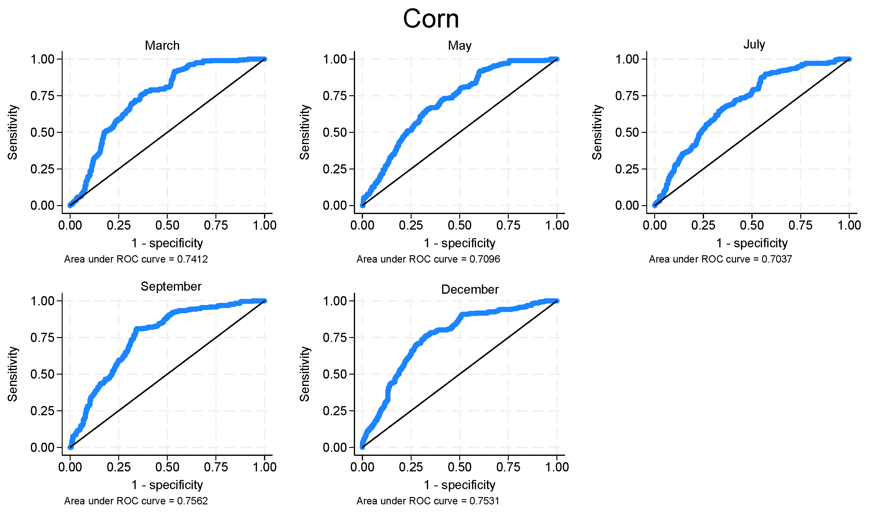
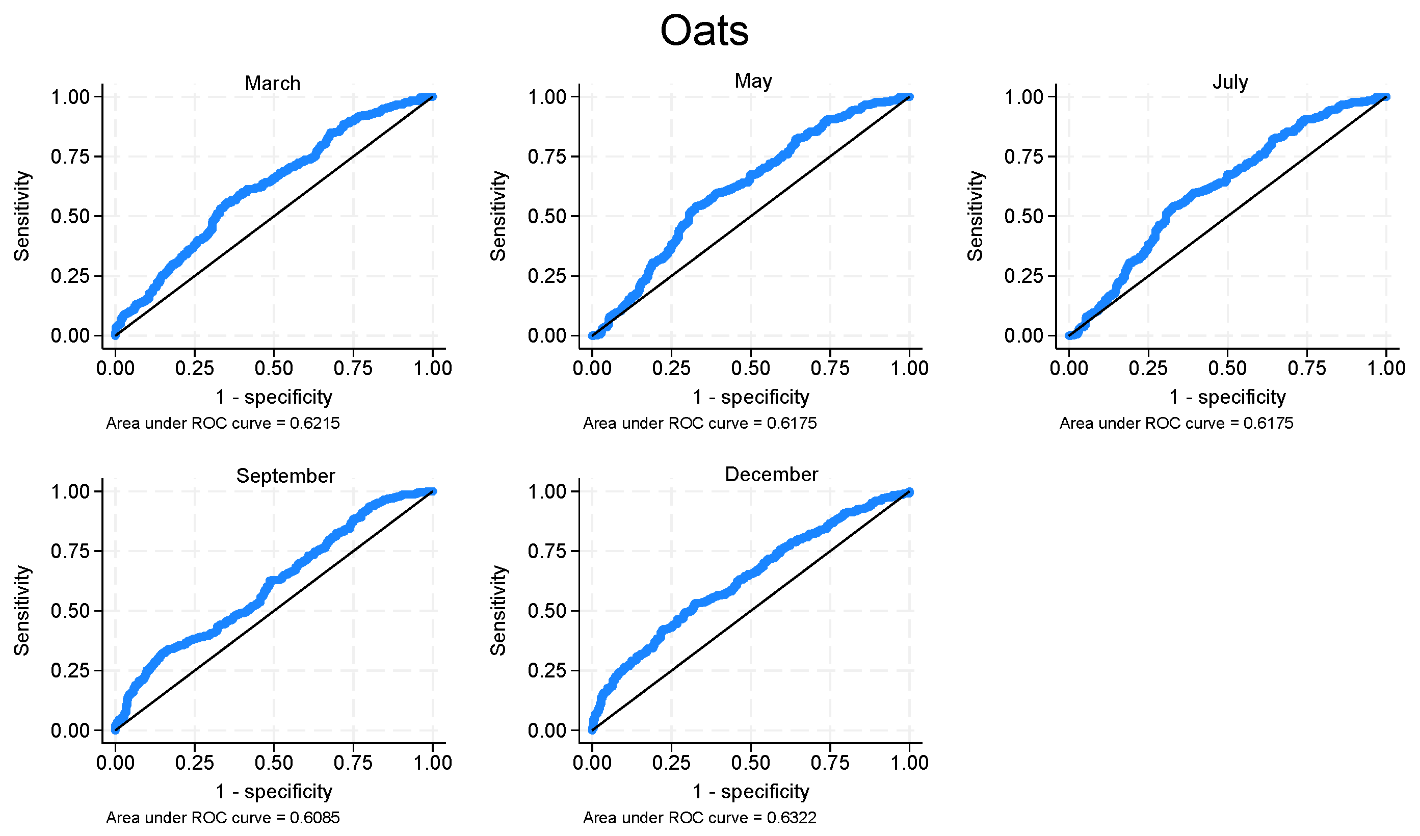
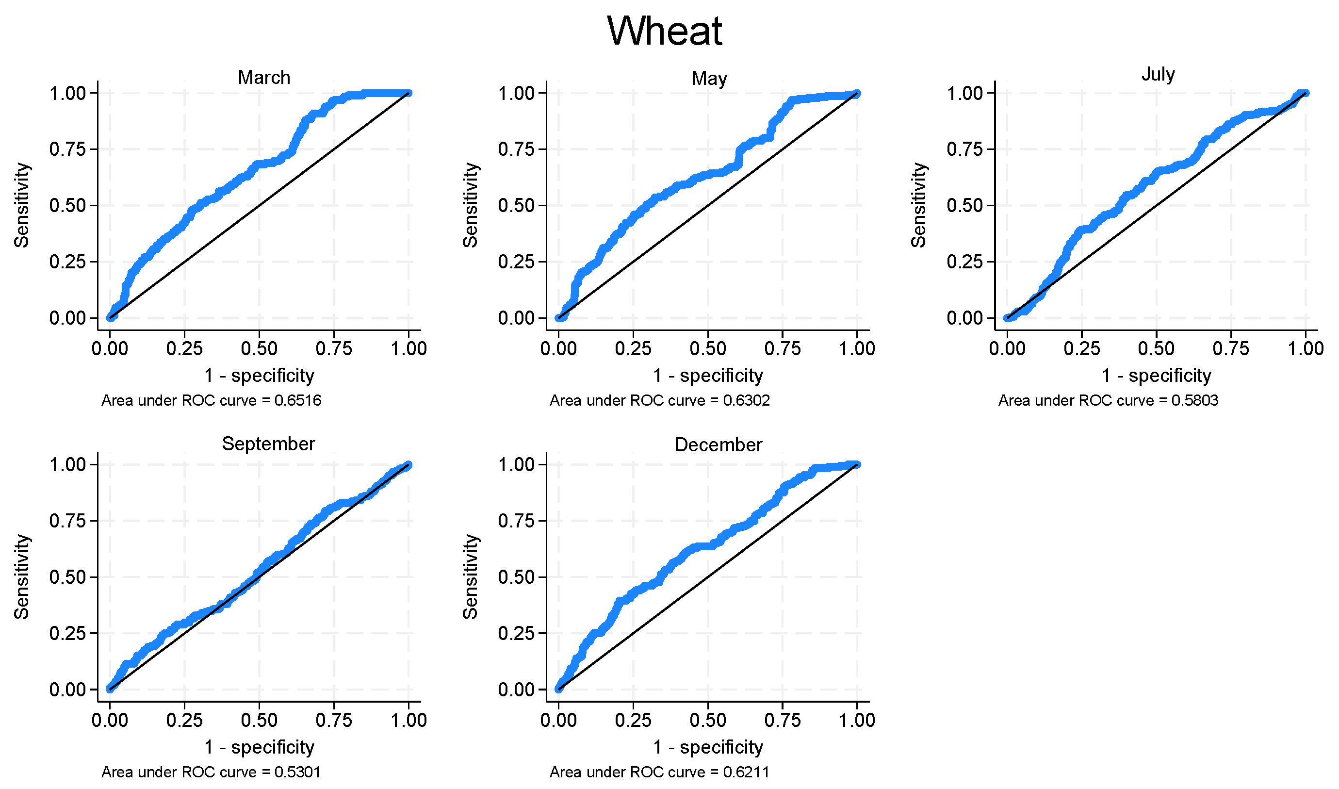
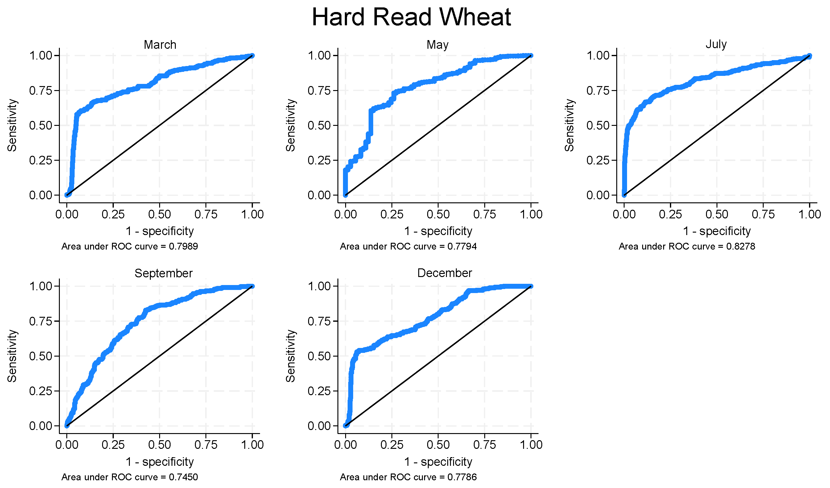
In this section, we present the ROC curves for each commodity and for each contract. A model with no predictive power would be a 45° line. The greater the predictive power, the more bowed the curve, and hence, the area beneath the curve is often used as a measure of the predictive power. A model with no predictive power has an area of 0.5; a perfect model has an area of 1. Figure 7, Figure 8, Figure 9, Figure 10, Figure 11 and Figure 12 provide the graphical representation of the ROC curves by commodities and contracts.
Table 12 reports the results relative to the area under the ROC curve for the agricultural commodities and future contract maturities. Regarding the kinds of commodities, we find important differences across them. In particular, we find that Hard Red Wheat (78.59%) and Soybeans (76.81%) show the highest discriminative power, while Wheat and Oats exhibit weaker performance, 60.27% and 61.96%, respectively. A possible explanation is related to the difference in market liquidity, volatility, and the information content included in futures prices. When we focus on contract maturities, we find that March, May, and July contracts perform better, 72.16%, 70.81%, and 70.87%, respectively, while September contracts report only 63.78%. A possible explanation is the seasonal patterns that lead to thin market conditions.

6. Conclusions

We found robust results for the investigation of our hypothesis. First, identifying the presence of price backwardation and its stickiness, notably for corn and wheat, is expected. These are commodities with a global market, sensitive to the volatilities of supply and demand, but most importantly, responding to corporate procurement. Commodity futures give companies insurance for the future value of their outputs.
The interesting fact, beyond the presence of backwardation, was its intensity as shown by the β 3 . This led us to proceed with confidence to stage two, to investigate the determinants of stickiness in prices during backwardation. The most significant determinant was convenience yield interest risk found by G. B. Gorton et al. (2013) and Jo et al. (2022).
The findings of this study carry several important implications. First, for policymakers and regulators, a better understanding of persistent backwardation can inform the design of agricultural support policies, storage interventions, and international trade agreements aimed at mitigating food price volatility. Second, for market participants such as producers, traders, and food-processing firms, recognizing the structural drivers of backwardation can improve hedging strategies, contract design, and procurement decisions. Third, for financial institutions and investors, insights into the stickiness of backwardation can help refine portfolio allocation, risk assessment, and the evaluation of commodities as an asset class. Finally, at a broader level, these results highlight the interconnectedness of agricultural markets with global food security and macroeconomic stability, underscoring the need for a coordinated approach to managing commodity price risks.
Our value added is in extending this reasoning over a longer period of time, but more importantly, identifying the time frame, the “when” of the occurrence. Future work will continue to investigate [i] the reasons behind the when/the occurrence and any new determinants from the dual theories of storage and normal backwardation that are the causes of this stickiness; and [ii] the mismatch between observed cash prices and futures contracts that introduce non-convergence risk and basis variability, especially close to delivery periods.

Author Contributions

P.C.: Writing—review & editing, Software, Methodology, Writing—original draft, Validation, Supervision, Methodology, Investigation, Data curation, Conceptualization. A.J.-D.: Writing—review & editing, Writing—original draft, Investigation, Formal analysis. G.Z.: Writing—review & editing, Funding, Writing—original draft, Validation, Supervision, Methodology, Investigation, Data curation, Conceptualization. All authors have read and agreed to the published version of the manuscript.

Funding

This research received no external funding.

Data Availability Statement

Data are available upon request from the authors.

Acknowledgments

We wish to thank two anonymous Referees for their insightful comments and suggestions provided in the previous version of the paper, and the participants in the European Financial Management Association conference (7–9 June 2023, Aalborgh, Denmark), in particular Andrei Stancu, Efraim Benmelech and Marie-Helene Gagnon for their very helpful comments and suggestions. Special thanks to Maurizio Mazziero and Lalith Samarakoon for their very valuable and constructive comments, which greatly helped to improve the paper. This research started when Peter Cincinelli was visiting the Department of Finance of the University of St. Thomas (Opus College of Business), Minneapolis (USA) in July 2019: financial support from the Outgoing Visiting Professors Scheme of University of Bergamo (Italy) is gratefully acknowledged. The usual disclaimer applies.

Conflicts of Interest

The authors declare no conflicts of interest.

Notes

1
Spot prices aggregate market information from various U.S. regional cash markets. They represent monthly prices reported for standard-quality grain delivered to the main regional terminal markets, and they are quoted in U.S. cents per bushel.
2
See: https://www.barchart.com/futures/major-commodities (accessed on 1 September 2022).
3
We thank a Referee for these insightful suggestions.

References

  1. Awokuse, T. O. (2005). Impact of macroeconomic policies on agricultural prices. Agricultural and Resource Economics Review, 34(2), 226–237. [Google Scholar] [CrossRef]
  2. Baldi, L., Peri, M., & Vandone, D. (2011, August 30–September 2). Price discovery in agricultural commodities: The shifting relationship between spot and future prices (Tech. Rep.). 2011 International Congress, Zurich, Switzerland. [Google Scholar]
  3. Bobenrieth, E., Wright, B., & Zeng, D. (2013). Stocks-to-use ratios and prices as indicators of vulnerability to spikes in global cereal markets. Agricultural Economics, 44(s1), 43–52. [Google Scholar] [CrossRef]
  4. Bopp, A. E., & Lady, G. M. (1991). A comparison of petroleum futures versus spot prices as predictors of prices in the future. Energy Economics, 13(4), 274–282. [Google Scholar] [CrossRef]
  5. Bordo, M. D. (1980). The effects of monetary change on relative commodity prices and the role of long-term contracts. Journal of Political Economy, 88(6), 1088–1109. [Google Scholar] [CrossRef]
  6. Brennan, M. J. (1958). The supply of storage. The American Economic Review, 48(1), 50–72. [Google Scholar]
  7. Chambers, R. G., & Just, R. E. (1982). An investigation of the effect of monetary factors on agriculture. Journal of Monetary Economics, 9(2), 235–247. [Google Scholar] [CrossRef]
  8. Cincinelli, P., Damiani, A. J., Jaiswal-Dale, A., & Zanotti, G. (2021). Booms in agricultural & non-agricultural prices: Who is responsible? Journal of Accounting & Finance, 21(3), 82–98. [Google Scholar]
  9. Cooper, R. N., Lawrence, R. Z., Bosworth, B., & Houthakker, H. S. (1975). The 1972–75 commodity boom. Brookings Papers on Economic Activity, 1975(3), 671–723. [Google Scholar] [CrossRef]
  10. Crain, S. J., & Lee, J. H. (1996). Volatility in wheat spot and futures markets, 1950–1993: Government farm programs, seasonality, and causality. The Journal of Finance, 51(1), 325–343. [Google Scholar]
  11. Dawson, P. J., Sanjuán, A. I., & White, B. (2006). Structural breaks and the relationship between barley and wheat futures prices on the London International Financial Futures Exchange. Review of Agricultural Economics, 28(4), 585–594. [Google Scholar] [CrossRef]
  12. Dimpfl, T., Flad, M., & Jung, R. C. (2017). Price discovery in agricultural commodity markets in the presence of futures speculation. Journal of Commodity Markets, 5, 50–62. [Google Scholar] [CrossRef]
  13. Fama, E. F., & French, K. R. (1987). Commodity futures prices: Some evidence on forecast power, premiums, and the theory of storage. Journal of Business, 60(1), 55–73. [Google Scholar] [CrossRef]
  14. Fleming, J., & Ostdiek, B. (1999). The impact of energy derivatives on the crude oil market. Energy Economics, 21(2), 135–167. [Google Scholar] [CrossRef]
  15. Garbade, K. D., & Silber, W. L. (1983). Price movements and price discovery in futures and cash markets. The Review of Economics and Statistics, 65(2), 289–297. [Google Scholar] [CrossRef]
  16. Garcia, P., & Leuthold, R. M. (2004). A selected review of agricultural commodity futures and options markets. European Review of Agricultural Economics, 31(3), 235–272. [Google Scholar] [CrossRef]
  17. Gerety, M. S., & Mulherin, J. H. (1991). Patterns in intraday stock market volatility, past and present. Financial Analysts Journal, 47(5), 71–79. [Google Scholar] [CrossRef]
  18. Ghosh, J. (2010). The unnatural coupling: Food and global finance. Journal of Agrarian Change, 10(1), 72–86. [Google Scholar] [CrossRef]
  19. Gilbert, C. L. (2010). How to understand high food prices. Journal of Agricultural Economics, 61(2), 398–425. [Google Scholar] [CrossRef]
  20. Giot, P. (2003). The information content of implied volatility in agricultural commodity markets. Journal of Futures Markets: Futures, Options, and Other Derivative Products, 23(5), 441–454. [Google Scholar] [CrossRef]
  21. Gorton, G., & Rouwenhorst, K. G. (2006). Facts and fantasies about commodity futures. Financial Analysts Journal, 62(2), 47–68. [Google Scholar] [CrossRef]
  22. Gorton, G. B., Hayashi, F., & Rouwenhorst, K. G. (2013). The fundamentals of commodity futures returns. Review of Finance, 17(1), 35–105. [Google Scholar] [CrossRef]
  23. Goswami, A., Adjemian, M. K., & Karali, B. (2022). The impact of futures contract storage rate policy on convergence expectations in domestic commodity markets. Food Policy, 111, 102301. [Google Scholar] [CrossRef]
  24. Hakkio, C. S., & Rush, M. (1989). Market efficiency and cointegration: An application to the sterling and deutschemark exchange markets. Journal of International Money and Finance, 8(1), 75–88. [Google Scholar] [CrossRef]
  25. Headey, D., & Fan, S. (2008). Anatomy of a crisis: The causes and consequences of surging food prices. Agricultural Economics, 39, 375–391. [Google Scholar] [CrossRef]
  26. Hernandez, M., & Torero, M. (2010). Examining the dynamic relationship between spot and future prices of agricultural commodities (Tech. Rep.). International Food Policy Research Institute (IFPRI). [Google Scholar]
  27. Hull, J. C. (2003). Options futures and other derivatives. Pearson Education India. [Google Scholar]
  28. Irwin, S. H., Garcia, P., Good, D. L., & Kunda, E. L. (2011). Spreads and non-convergence in Chicago Board of Trade corn, soybean, and wheat futures: Are index funds to blame? Applied Economic Perspectives and Policy, 33(1), 116–142. [Google Scholar] [CrossRef]
  29. Irwin, S. H., & Sanders, D. R. (2011). Index funds, financialization, and commodity futures markets. Applied Economic Perspectives and Policy, 33(1), 1–31. [Google Scholar] [CrossRef]
  30. Jo, Y., Kim, J., & Santos, F. (2022). The impact of liquidity risk in the Chinese banking system on the global commodity markets. Journal of Empirical Finance, 66, 23–50. [Google Scholar] [CrossRef]
  31. Kuiper, W. E., Pennings, J. M., & Meulenberg, M. T. (2002). Identification by full adjustment: Evidence from the relationship between futures and spot prices. European Review of Agricultural Economics, 29(1), 67–84. [Google Scholar] [CrossRef]
  32. Martin, L., & Garcia, P. (1981). The price-forecasting performance of futures markets for live cattle and hogs: A disaggregated analysis. American Journal of Agricultural Economics, 63(2), 209–215. [Google Scholar] [CrossRef]
  33. Maslyuk, S., & Smyth, R. (2009). Cointegration between oil spot and future prices of the same and different grades in the presence of structural change. Energy Policy, 37(5), 1687–1693. [Google Scholar] [CrossRef]
  34. Masters, M. W. (2008, May 20). Testimony before the committee on homeland security and governmental affairs. US Senate. [Google Scholar]
  35. Mohan, S., & Love, J. (2004). Coffee futures: Role in reducing coffee producers’ price risk. Journal of International Development, 16(7), 983–1002. [Google Scholar] [CrossRef]
  36. Moosa, I. A., & Al-Loughani, N. E. (1994). Unbiasedness and time varying risk premia in the crude oil futures market. Energy Economics, 16(2), 99–105. [Google Scholar] [CrossRef]
  37. Quan, J. (1992). Two-step testing procedure for price discovery role of futures prices. The Journal of Futures Markets (1986–1998), 43(1), 139. [Google Scholar] [CrossRef]
  38. Robles, M., & Cooke, B. (2009). Recent food prices movements: A time series analysis. International Food Policy Research Institute. [Google Scholar]
  39. Sanders, D. R., & Irwin, S. H. (2010). A speculative bubble in commodity futures prices? Cross-sectional evidence. Agricultural Economics, 41(1), 25–32. [Google Scholar] [CrossRef]
  40. Serletis, A. (1991). Rational expectations, risk and efficiency in energy futures markets. Energy Economics, 13(2), 111–115. [Google Scholar] [CrossRef]
  41. Silvapulle, P., & Moosa, I. A. (1999). The relationship between spot and futures prices: Evidence from the crude oil market. Journal of Futures Markets: Futures, Options, and Other Derivative Products, 19(2), 175–193. [Google Scholar] [CrossRef]
  42. Stoll, H. R., & Whaley, R. E. (2010). Commodity index investing and commodity futures prices. Journal of Applied Finance (Formerly Financial Practice and Education), 20(1). Available online: https://ssrn.com/abstract=2693084 (accessed on 1 September 2022). [CrossRef]
  43. Tang, K., & Xiong, W. (2010). VIndex investment and financialization of commoditiesV. NBER Working Paper w16385. NBER. [Google Scholar]
  44. Taylor, J. B. (1995). The monetary transmission mechanism: An empirical framework. Journal of Economic Perspectives, 9(4), 11–26. [Google Scholar] [CrossRef]
  45. Telser, L. G. (1958). Futures trading and the storage of cotton and wheat. Journal of Political Economy, 66(3), 233–255. [Google Scholar] [CrossRef]
  46. Triantafyllou, A., Dotsis, G., & Sarris, A. (2020). Assessing the vulnerability to price spikes in agricultural commodity markets. Journal of Agricultural Economics, 71(3), 631–651. [Google Scholar] [CrossRef]
  47. Wahab, M., & Lashgari, M. (1993). Price dynamics and error correction in stock index and stock index futures markets: A cointegration approach. Journal of Futures Markets, 13(7), 711–742. [Google Scholar] [CrossRef]
  48. Working, H. (1948). Theory of the inverse carrying charge in futures markets. Journal of Farm Economics, 30(1), 1–28. [Google Scholar] [CrossRef]
  49. Yang, J., Bessler, D. A., & Leatham, D. J. (2001). Asset storability and price discovery in commodity futures markets: A new look. Journal of Futures Markets: Futures, Options, and Other Derivative Products, 21(3), 279–300. [Google Scholar] [CrossRef]
Figure 1. Corn—Spot and Future Monthly Prices. The figure shows the monthly time series of corn spot prices (red lines) and futures prices (blue lines) across five contract maturities (March, May, July, September, and December), and the estimation of growth equations for each contract to analyze price dynamics. Source: Authors’ elaboration from BarChart database.
Jrfm 18 00674 g001
Figure 2. Oats—Spot and Future Monthly Prices. The figure shows the monthly time series of oats spot prices (red lines) and futures prices (blue lines) across five contract maturities (March, May, July, September, and December), and the estimation of growth equations for each contract to analyze price dynamics. Source: Authors’ elaboration from BarChart database.
Jrfm 18 00674 g002
Figure 3. Soybeans—Spot and Future Monthly Prices. The figure shows the monthly time series of soybeans spot prices (red lines) and futures prices (blue lines) across five contract maturities (March, May, July, September, and September), and the estimation of growth equations for each contract to analyze price dynamics. Source: Authors’ elaboration from BarChart database.
Jrfm 18 00674 g003
Figure 4. Soybean Oil—Spot and Future Monthly Prices. The figure shows the monthly time series of soybean oil spot prices (red lines) and futures prices (blue lines) across five contract maturities (March, May, July, September, and December), and the estimation of growth equations for each contract to analyze price dynamics. Source: Authors’ elaboration from BarChart database.
Jrfm 18 00674 g004
Figure 5. Wheat—Spot and Future Monthly Prices. The figure shows the monthly time series of wheat spot prices (red lines) and futures prices (blue lines) across five contract maturities (March, May, July, September, and December), and the estimation of growth equations for each contract to analyze price dynamics. Source: Authors’ elaboration from BarChart database.
Jrfm 18 00674 g005
Figure 6. Hard Red Wheat—Spot and Future Monthly Prices. The figure shows the monthly time series of hard red wheat spot prices (red lines) and futures prices (blue lines) across five contract maturities (March, May, July, September, and December), and the estimation of growth equations for each contract to analyze price dynamics. Source: Authors’ elaboration from BarChart database.
Jrfm 18 00674 g006
Figure 7. Corn—Area under the ROC curve. Source: Authors elaboration from BarChart database.
Jrfm 18 00674 g007
Figure 8. Oats—Area under the ROC curve. Source: Authors’ elaboration from BarChart database.
Jrfm 18 00674 g008
Figure 9. Soybeans—Area under the ROC curve. Source: Authors’ elaboration from BarChart database.
Jrfm 18 00674 g009
Figure 10. Soybean Oil—Area under the ROC curve. Source: Authors’ elaboration from BarChart database.
Jrfm 18 00674 g010
Figure 11. Wheat—Area under the ROC curve. Source: Authors’ elaboration from BarChart database.
Jrfm 18 00674 g011
Figure 12. Hard Read Wheat—Area under the ROC curve. Source: Authors’ elaboration from BarChart database.
Jrfm 18 00674 g012
Table 1. Stickiness persistence in backwardation. Future Prices—March contracts.
Dep. Variable: Spot PriceCornOatsSoybeansSoybean OilWheatHar Red Wheat
[i][ii][iii][iv][v][vi]
ln Future Pricest−20.9196 ***0.7737 ***0.9157 ***0.9752 ***0.8270 ***0.9421 ***
(0.0451)(0.0599)(0.0465)(0.0327)(0.0486)(0.0388)
Backwardation dummyt−0.37940.1768−0.17540.0875−0.12760.7097 *
(0.2399)(0.3183)(0.2764)(0.1591)(0.2688)(0.3843)
(Backwardation dummy × log Future Prices)t−20.0782 *−0.01140.03760.01880.0418−0.0902
(0.0411)(0.0583)(0.0405)(0.0457)(0.0435)(0.0625)
VIXt−20.001−0.00140.0016 **0.0008−0.0022 **0.0021 **
(0.0009)(0.0011)(0.0008)(0.0008)(0.0010)(0.0009)
CPIt−20.0008 **0.0023 ***0.00020.0008 **0.0016 ***0.0006
(0.0003)(0.0004)(0.0004)(0.0003)(0.0004)(0.0004)
T-billt−2−0.0081−0.0058−0.0202 ***−0.0007−0.00050.0139 **
(0.0059)(0.0055)(0.0059)(0.0060)(0.0072)(0.0068)
Constant0.25370.7800 **0.5061 *−0.16260.6573 **0.0782
(0.2327)(0.3267)(0.2877)(0.1395)(0.2672)(0.2720)
N. Obs.270270270270270270
R2 Adj.0.920.890.930.930.830.84
F-Test198.84 ***173.33 ***235.74 ***216.42 ***131.59 ***174.10 ***
The table reports the results for stickiness persistence in backwardation for future prices—March contracts. Spot Pricesi,t represents monthly commodities spot prices; Future Pricesi,t−2 represents monthly commodities future contract prices; Backwardation Dummy, takes the value of 1 when spot prices are greater than future prices, between t 1 and t, and 0 otherwise. X t 2 is a vector of explanatory variables such as the following: V I X t 2 is the Chicago Board Options Exchange’s (CBOE) Volatility Index, a measure of the stock market’s expectation of volatility based on S&P 500 index options; C P I t 2 is the monthly US Consumer Price Index ratio; T B i l l t 1 is the 3-month US treasury bill. Standard errors are robust and reported in parentheses. *, **, *** denote the 10%, 5% and 1% significance level, respectively.
Table 2. Stickiness persistence in backwardation. Future Prices—September contracts.
Dep. Variable: Spot PriceCornOatsSoybeansSoybean OilWheatHard Red Wheat
[i][ii][iii][iv][v][vi]
ln Future Pricest−2 (September)0.9201 ***0.8228 ***0.9127 ***0.9822 ***0.8458 ***0.9786 ***
(0.0461)(0.0606)(0.0491)(0.0331)(0.0505)(0.0419)
Backwardation dummyt−0.5291 *0.38460.07270.16420.33950.5697
(0.2758)(0.3306)(0.2710)(0.1668)(0.3524)(0.4781)
(Backwardation dummy × log Future Prices)t−20.1048 **−0.03840.0088−0.0028−0.0338−0.0635
(0.0465)(0.0606)(0.0398)(0.0484)(0.0575)(0.0772)
VIXt−20.0008−0.00060.00090.0012−0.0028 **0.0016
(0.0009)(0.0012)(0.0009)(0.0009)(0.0010)(0.0011)
CPIt−20.0008 **0.0018 ***0.00060.0009 **0.0013 **0.0002
(0.0004)(0.0005)(0.0003)(0.0004)(0.0005)(0.0006)
T-billt−2−0.0072−0.0081−0.00890.001−0.00360.0162 **
(0.0058)(0.0062)(0.0055)(0.0062)(0.0071)(0.0068)
Constant0.23880.5728 *0.4199−0.22750.6299 **−0.0598
(0.2358)(0.3366)(0.2935)(0.1492)(0.2841)(0.3262)
N. Obs.270270270270270270
R2 Adj.0.920.870.930.930.830.84
F-Test196.95 ***146.38 ***239.90 ***210.74 ***132.92 ***176.79 ***
The table reports the results for stickiness persistence in backwardation for future prices—September contracts. Spot Pricesi,t represents monthly commodities spot prices; Future Pricesi,t−2 represents monthly commodities future contract prices; Backwardation Dummy, takes the value of 1 when spot prices are greater than future prices, between t 1 and t, and 0 otherwise. X t 2 is a vector of explanatory variables such as the following: V I X t 2 is the Chicago Board Options Exchange’s (CBOE) Volatility Index, a measure of the stock market’s expectation of volatility based on S&P 500 index options; C P I t 2 is the monthly US Consumer Price Index ratio; T B i l l t 1 is the 3-month US treasury bill. Standard errors are robust and reported in parentheses. *, **, *** denote the 10%, 5% and 1% significance level, respectively.
Table 3. Stickiness persistence in backwardation. Future Prices—December contracts.
Dep. Variable: Spot PriceCornOatsSoybean OilWheatHard Red Wheat
[i][ii][iii][iv][v]
ln Future Pricest−20.9122 ***0.8229 ***0.9821 ***0.8451 ***0.9721 ***
(0.0507)(0.0634)(0.0338)(0.0470)(0.0425)
Backwardation dummyt−0.4566 *0.5923 *0.2951 *0.10971.0496**
(0.2758)(0.3460)(0.1645)(0.3545)(0.4253)
(Backwardation dummy × log Future Prices)t−20.0946 **−0.0889−0.03830.0031−0.1449 **
(0.0473)(0.0636)(0.0478)(0.0577)(0.0686)
VIXt−20.001−0.00160.0011−0.0032 **0.0026 **
(0.0009)(0.0011)(0.0009)(0.0011)(0.0012)
CPIt−20.0010 **0.0025 ***0.0012 **0.0015 ***0.0009 *
(0.0004)(0.0004)(0.0004)(0.0004)(0.0005)
T-billt−2−0.0071−0.00660.0024−0.00390.0209 **
(0.0062)(0.0060)(0.0061)(0.0073)(0.0072)
Constant0.24140.4802−0.2931 *0.6100 **−0.2004
(0.2647)(0.3553)(0.1517)(0.2660)(0.3225)
N. Obs.270270270270270
R2 Adj.0.910.870.930.820.84
F-Test185.26 ***152.35 ***208.7 ***129.58 ***169.71 ***
The table reports the results for stickiness persistence in backwardation for future prices—December contracts. Spot Pricesi,t represents monthly commodities spot prices; Future Pricesi,t−2 represents monthly commodities future contract prices; Backwardation Dummy, takes the value of 1 when spot prices are greater than future prices, between t 1 and t, and 0 otherwise. X t 2 is a vector of explanatory variables such as the following: V I X t 2 is the Chicago Board Options Exchange’s (CBOE) Volatility Index, a measure of the stock market’s expectation of volatility based on S&P 500 index options; C P I t 2 is the monthly US Consumer Price Index ratio; T B i l l t 1 is the 3-month US treasury bill. Standard errors are robust and reported in parentheses. *, **, *** denote the 10%, 5% and 1% significance level, respectively.
Table 4. Stickiness persistence in backwardation. Future Prices—May contracts.
Dep. Variable: Spot PriceCornOatsSoybeansSoybean OilWheatHard Red Wheat
[i][ii][iii][iv][v][vi]
ln Future Pricest−20.9315 ***0.8349 ***0.9469 ***0.9700 ***0.8009 ***0.9271 ***
(0.0409)(0.0599)(0.0448)(0.0339)(0.0524)(0.0385)
Backwardation dummyt−0.25670.5208 *0.3940.20740.08730.6422
(0.2163)(0.2889)(0.2566)(0.1760)(0.2607)(0.3981)
(Backwardation dummy × log Future Prices)t−20.0515−0.0748−0.0466−0.01670.0059−0.0789
(0.0370)(0.0527)(0.0374)(0.0510)(0.0425)(0.0645)
VIXt−20.0016 *−0.00140.0018 **0.0009−0.00120.0020 **
(0.0009)(0.0009)(0.0007)(0.0008)(0.0010)(0.0010)
CPIt−20.0008 **0.0022 ***0.00030.0010 **0.0020 ***0.0006
(0.0003)(0.0004)(0.0004)(0.0003)(0.0004)(0.0005)
T-billt−2−0.0091−0.0057−0.0151 **0.00070.00090.0112 *
(0.0056)(0.0051)(0.0051)(0.0061)(0.0076)(0.0066)
Constant0.16330.45510.2496−0.1950.7256 **0.1858
(0.2191)(0.3105)(0.2613)(0.1463)(0.2817)(0.2723)
N. Obs.270270270270270270
R2 Adj.0.920.890.930.930.810.83
F-Test199.38 ***174.80 ***242.14 ***220.45 ***121.84 ***164.34 ***
The table reports the results for stickiness persistence in backwardation for future prices—May contracts. Spot Pricesi,t represents monthly commodities spot prices; Future Pricesi,t−2 represents monthly commodities future contract prices; Backwardation Dummy, takes the value of 1 when spot prices are greater than future prices, between t 1 and t, and 0 otherwise. X t 2 is a vector of explanatory variables such as the following: V I X t 2 is the Chicago Board Options Exchange’s (CBOE) Volatility Index, a measure of the stock market’s expectation of volatility based on S&P 500 index options; C P I t 2 is the monthly US Consumer Price Index ratio; T B i l l t 1 is the 3-month US treasury bill. Standard errors are robust and reported in parentheses. *, **, *** denote the 10%, 5% and 1% significance level, respectively.
Table 5. Stickiness persistence in backwardation. Future Prices—July contracts.
Dep. Variable: Spot PriceCornOatsSoybeansSoybean OilWheatHard Red Wheat
[i][ii][iii][iv][v][vi]
ln Future Pricest−20.9421 ***0.8049 ***0.9108 ***0.9670 ***0.8227 ***0.9484 ***
(0.0391)(0.0657)(0.0414)(0.0343)(0.0586)(0.0419)
Backwardation dummyt−0.07740.27640.2230.0950.10930.4554
(0.2299)(0.3387)(0.3090)(0.1787)(0.3189)(0.4498)
(Backwardation dummy × log Future Prices)t−20.0236−0.0298−0.02010.01360.0084−0.0434
(0.0388)(0.0615)(0.0442)(0.0517)(0.0519)(0.0729)
VIXt−20.0013 *−0.0018 *0.0016 **0.0008−0.00130.0005
(0.0008)(0.0011)(0.0008)(0.0008)(0.0010)(0.0010)
CPIt−20.0007 **0.0018 ***0.00040.0008 **0.0017 ***0.0002
(0.0003)(0.0004)(0.0004)(0.0003)(0.0004)(0.0005)
T-billt−2−0.008−0.0102 *−0.0155 **−0.00260.00180.0106
(0.0050)(0.0059)(0.0053)(0.0063)(0.0076)(0.0070)
Constant0.12870.7198 **0.4692 *−0.12190.6401 *0.1631
(0.2092)(0.3577)(0.2491)(0.1531)(0.3251)(0.3159)
N. Obs.270270270270270270
R2 Adj.0.920.890.930.930.820.83
F-Test212.84 ***159.53 ***236.37 ***213.32 ***128.64 ***167.81 ***
The table reports the results for stickiness persistence in backwardation for future prices—July contracts. Spot Pricesi,t represents monthly commodities spot prices; Future Pricesi,t−2 represents monthly commodities future contract prices; Backwardation Dummy, takes the value of 1 when spot prices are greater than future prices, between t 1 and t, and 0 otherwise. X t 2 is a vector of explanatory variables such as the following: V I X t 2 is the Chicago Board Options Exchange’s (CBOE) Volatility Index, a measure of the stock market’s expectation of volatility based on S&P 500 index options; C P I t 2 is the monthly US Consumer Price Index ratio; T B i l l t 1 is the 3-month US treasury bill. Standard errors are robust and reported in parentheses. *, **, *** denote the 10%, 5% and 1% significance level, respectively.
Table 6. Determinant of stickiness persistence—Commodity: Corn.
CornMarchMayJulySeptemberDecember
[i][ii][iii][iv][v]
March Convenience Yieldt−1−0.4499 ***
(0.0477)
May Convenience Yieldt−1 −0.3619 ***
(0.0418)
July Convenience Yieldt−1 −0.3090 ***
(0.0397)
September Convenience Yieldt−1 −0.3731 ***
(0.0398)
December Convenience Yieldt−1 −0.3381 ***
(0.0363)
Interest Riskt−10.20050.194−0.061−0.8848 ***−0.8951 ***
(0.2180)(0.2045)(0.2193)(0.2435)(0.2400)
S&P 500 returnst−1−3.5524 *0.0576−2.18531.29332.4126
(2.0078)(1.9425)(1.9670)(1.9847)(2.0098)
Δ Baltic Dry Indext−1−0.0002−0.00010.00000.00000.0000
(0.0002)(0.0002)(0.0002)(0.0002)(0.0002)
VIXt−1−0.0191 **−0.0024−0.0140 **0.0101−0.0001
(0.0061)(0.0065)(0.0062)(0.0063)(0.0060)
Constant0.4818 ***−0.03440.17640.2637 **0.4396 ***
(0.1231)(0.1239)(0.1214)(0.1232)(0.1227)
N. Obs.907907907907907
Pseudo R20.150.100.090.160.14
Log-Likelihood−499.06 ***−505.05 ***−505.26 ***−510.94 ***−522.38 ***
The table reports the results for the determinant of stickiness persistence for Corn. Y t , the dependent variable, takes value 1 when a time series shows backwardation and 0 otherwise; X t 1 is a vector of monthly explanatory variables such as C o n v e n i e n c e Y i e l d t 1 defined as follows: C o n v e n i e n c e Y i e l d = ln ( F ( t , T 1 ) ) ln ( F ( t , T 2 ) ) T 2 T 1 + γ t , where F ( t , T 1 ) and F ( t , T 2 ) are futures prices at month t with maturity T 1 and T 2 , respectively; γ t denotes the local interest rate Libor for US; I n t e r e s t   R a t e R i s k t 1 is the difference between 3-month Libor and overnight 3-month Libor for US; S & P 500 r e t u r n s t 1 is the monthly returns of S&P 500; B a l t i c D r y I n d e x C h a n g e t 1 is the monthly change in Baltic Dry index; V I X t 2 is the Chicago Board Options Exchange’s (CBOE) Volatility Index, a measure of the stock market’s expectation of volatility based on S&P 500 index options. Standard errors are robust and reported in parentheses. *, **, *** denote the 10%, 5% and 1% significance level, respectively.
Table 7. Determinant of stickiness persistence—Commodity: Wheat.
WheatMarchMayJulySeptemberDecember
[i][ii][iii][iv][v]
March Convenience Yieldt−1−0.3165 ***
(0.0538)
March Convenience Yieldt−1 −0.2091 ***
(0.0429)
March Convenience Yieldt−1 −0.0614**
(0.0298)
March Convenience Yieldt−1 −0.0008
(0.0312)
March Convenience Yieldt−1 −0.1114 **
(0.0412)
Interest Riskt−1−0.05240.1592−0.5842 **−0.6469 **−0.5398 **
(0.2215)(0.2194)(0.1997)(0.2179)(0.2161)
S&P500 returnst−10.8114−0.43020.47423.3523 *5.4663 **
(2.2273)(2.2142)(1.9174)(2.0369)(2.0799)
Δ Dry Indext−1−0.0005 **0−0.0001−0.0001−0.0004 *
(0.0002)(0.0002)(0.0002)(0.0002)(0.0002)
VIXt−1−0.0098−0.0189 **−0.0037−0.00360.0085
(0.0071)(0.0077)(0.0062)(0.0065)(0.0067)
VSRt1.1937 ***0.9975 ***0.8395 ***1.2960 ***1.4901 ***
(0.1109)(0.1035)(0.0997)(0.1036)(0.1095)
Kraft squeezet1.2024 **0.00000.00000.0000−0.1018
(0.4107)(0.0000)(0.0000)(0.0000)(0.5379)
Constant−0.6118 ***−0.4068 **−0.2999 **−0.7607 ***−1.2026 ***
(0.1486)(0.1525)(0.1327)(0.1492)(0.1533)
N. Obs.907898898898907
Pseudo R20.190.130.080.160.24
Log-Likelihood−388.73 ***−437.84 ***−538.67 ***−448.74 ***−358.39 ***
The table reports the results for the determinant of stickiness persistence for Wheat. Y t , the dependent variable, takes value 1 when a time series shows backwardation and 0 otherwise; X t 1 is a vector of monthly explanatory variables such as C o n v e n i e n c e Y i e l d t 1 defined as follows: C o n v e n i e n c e Y i e l d = ln ( F ( t , T 1 ) ) ln ( F ( t , T 2 ) ) T 2 T 1 + γ t , where F ( t , T 1 ) and F ( t , T 2 ) are futures prices at month t with maturity T 1 and T 2 , respectively; γ t denotes the local interest rate Libor for US; I n t e r e s t   R a t e R i s k t 1 : is the difference between 3-month Libor and overnight 3-month Libor for US; S & P 500 r e t u r n s t 1 is the monthly returns of S&P 500; B a l t i c D r y I n d e x C h a n g e t 1 is the monthly change in Baltic Dry index; V I X t 2 is the Chicago Board Options Exchange’s (CBOE) Volatility Index, a measure of the stock market’s expectation of volatility based on S&P 500 index options; VSR is the Variable Storage Rate: a dummy variable that is equal to 1 during the period from July 2010 to August 2022 for wheat. Kraft squeeze is a dummy variable equal to 1 for March 2008 and December 2011, 0 otherwise. Standard errors are robust and reported in parentheses. *, **, *** denote the 10%, 5% and 1% significance level, respectively.
Table 8. Determinant of stickiness persistence—Commodity: Soybeans.
SoybeansMarchMayJulySeptember
[i][ii][iii][iv]
March Convenience Yieldt−1−0.7675 ***
(0.1195)
May Convenience Yieldt−1 −0.7178 ***
(0.1073)
July Convenience Yieldt−1 −0.9161 ***
(0.1688)
September Convenience Yieldt−1 −0.9098 ***
(0.1549)
Interest Riskt−11.3574 ***1.3670 ***1.6402 ***0.9730 **
(0.4048)(0.3178)(0.4119)(0.3631)
S&P 500 returnst−1−1.4573−1.416−0.76431.2038
(2.4700)(2.5313)(2.5907)(2.1176)
Δ Baltic Dry Indext−10.0003−0.00030.00000.0002
(0.0003)(0.0003)(0.0003)(0.0003)
VIXt−1−0.0266 **−0.0532 ***−0.0598 ***−0.0083
(0.0106)(0.0087)(0.0096)(0.0079)
Constant0.3086 *0.6477 ***0.7333 ***0.4470 **
(0.1790)(0.1604)(0.1778)(0.1563)
N. Obs.907907907907
Pseudo R20.200.190.220.27
Log-Likelihood−426.38 ***−401.24 ***−367.96 ***−433.31 ***
The table reports the results for the determinant of stickiness persistence for Soybeans. Y t , the dependent variable, takes value 1 when a time series shows backwardation and 0 otherwise; X t 1 is a vector of monthly explanatory variables such as C o n v e n i e n c e Y i e l d t 1 defined as follows: C o n v e n i e n c e Y i e l d = ln ( F ( t , T 1 ) ) ln ( F ( t , T 2 ) ) T 2 T 1 + γ t , where F ( t , T 1 ) and F ( t , T 2 ) are futures prices at month t with maturity T 1 and T 2 , respectively; γ t denotes the local interest rate Libor for US; I n t e r e s t   R a t e R i s k t 1 is the difference between 3-month Libor and overnight 3-month Libor for US; S & P 500 r e t u r n s t 1 is the monthly returns of S&P 500; B a l t i c D r y I n d e x C h a n g e t 1 is the monthly change in Baltic Dry index; V I X t 2 is the Chicago Board Options Exchange’s (CBOE) Volatility Index, a measure of the stock market’s expectation of volatility based on S&P 500 index options. Standard errors are robust and reported in parentheses. *, **, *** denote the 10%, 5% and 1% significance level, respectively.
Table 9. Determinant of stickiness persistence—Commodity: Soybean Oil.
Soybean OilMarchMayJulySeptemberDecember
[i][ii][iii][iv][v]
March Convenience Yieldt−1−0.2023 ***
(0.0326)
May Convenience Yieldt−1 −0.2454 ***
(0.0363)
July Convenience Yieldt−1 −0.2395 ***
(0.0349)
September Convenience Yieldt−1 −0.2292 ***
(0.0328)
December Convenience Yieldt−1 −0.2030 ***
(0.0315)
Interest Riskt−1−0.1983−0.0909−0.1089−0.118−0.2235
(0.2148)(0.2175)(0.2243)(0.2220)(0.2034)
S&P 500 returnst−1−0.866−0.6810.6677−0.6010.9485
(2.0878)(2.1068)(2.0692)(2.0873)(1.9863)
Δ Baltic Dry Indext−1−0.0002−0.0002−0.0002−0.0001−0.0001
(0.0002)(0.0002)(0.0002)(0.0002)(0.0002)
VIXt−1−0.0048−0.0022−0.0026−0.0084−0.0031
(0.0059)(0.0060)(0.0059)(0.0059)(0.0059)
Constant−0.3990 ***−0.5154 ***−0.5212 ***−0.3296 **−0.3307 **
(0.1163)(0.1156)(0.1157)(0.1177)(0.1155)
N. Obs.907907907907907
Pseudo R20.050.060.060.050.05
Log-Likelihood−442.23 ***−410.48 ***−408.35 ***−436.17 ***−471.20 ***
The table reports the results for the determinant of stickiness persistence for Soybean Oil. Y t , the dependent variable, takes value 1 when a time series shows backwardation and 0 otherwise; X t 1 is a vector of monthly explanatory variables such as C o n v e n i e n c e Y i e l d t 1 defined as follows: C o n v e n i e n c e Y i e l d = ln ( F ( t , T 1 ) ) ln ( F ( t , T 2 ) ) T 2 T 1 + γ t , where F ( t , T 1 ) and F ( t , T 2 ) are futures prices at month t with maturity T 1 and T 2 , respectively; γ t denotes the local interest rate Libor for US; I n t e r e s t   R a t e R i s k t 1 is the difference between 3-month Libor and overnight 3-month Libor for US; S & P 500 r e t u r n s t 1 is the monthly returns of S&P 500; B a l t i c D r y I n d e x C h a n g e t 1 is the monthly change in Baltic Dry index; V I X t 2 is the Chicago Board Options Exchange’s (CBOE) Volatility Index, a measure of the stock market’s expectation of volatility based on S&P 500 index options. Standard errors are robust and reported in parentheses. *, **, *** denote the 10%, 5% and 1% significance level, respectively.
Table 10. Determinant of stickiness persistence—Commodity: Oats.
OatsMarchMayJulySeptemberDecember
[i][ii][iii][iv][v]
March Convenience Yieldt−1−0.1370 ***
(0.0275)
May Convenience Yieldt−1 −0.1320 ***
(0.0263)
July Convenience Yieldt−1 −0.1320 ***
(0.0263)
September Convenience Yieldt−1 0.0857 **
(0.0277)
December Convenience Yieldt−1 0.1919 ***
(0.0323)
Interest Riskt−10.19210.23250.2325−0.6145 ***−0.4700 **
(0.2070)(0.1854)(0.1854)(0.1824)(0.2039)
S&P 500 returnst−1−1.0095−2.4191−2.41911.18963.6814 *
(2.0738)(1.9216)(1.9216)(1.8786)(1.8959)
Δ Baltic Dry Indext−10.00010.00010.00010.00010.0003
(0.0002)(0.0002)(0.0002)(0.0002)(0.0002)
VIXt−1−0.0303 ***−0.0323 ***−0.0323 ***−0.0150 **0.0134 **
(0.0069)(0.0065)(0.0065)(0.0063)(0.0066)
Constant0.3010 **0.5798 ***0.5798 ***0.6083 ***0.1951
(0.1321)(0.1256)(0.1256)(0.1250)(0.1265)
N. Obs.907907907907907
Pseudo R20.040.040.040.040.04
Log-Likelihood−557.88 ***−596.49 ***−596.49 ***−580.91 ***−512.60 ***
The table reports the results for the determinant of stickiness persistence for Oats. Y t , the dependent variable, takes value 1 when a time series shows backwardation and 0 otherwise; X t 1 is a vector of monthly explanatory variables such as C o n v e n i e n c e Y i e l d t 1 defined as follows: C o n v e n i e n c e Y i e l d = ln ( F ( t , T 1 ) ) ln ( F ( t , T 2 ) ) T 2 T 1 + γ t , where F ( t , T 1 ) and F ( t , T 2 ) are futures prices at month t with maturity T 1 and T 2 , respectively; γ t denotes the local interest rate Libor for US; I n t e r e s t   R a t e R i s k t 1 is the difference between 3-month Libor and overnight 3-month Libor for US; S & P 500 r e t u r n s t 1 is the monthly returns of S&P 500; B a l t i c D r y I n d e x C h a n g e t 1 is the monthly change in Baltic Dry index; V I X t 2 is the Chicago Board Options Exchange’s (CBOE) Volatility Index, a measure of the stock market’s expectation of volatility based on S&P 500 index options. Standard errors are robust and reported in parentheses. *, **, *** denote the 10%, 5% and 1% significance level, respectively.
Table 11. Determinant of stickiness persistence—Commodity: Hard Red Wheat.
Hard Red WheatMarchMayJulySeptemberDecember
[i][ii][iii][iv][v]
March Convenience Yieldt−10.5076 ***
(0.0316)
May Convenience Yieldt−1 0.3104 ***
(0.0485)
July Convenience Yieldt−1 0.6177 ***
(0.0332)
September Convenience Yieldt−1 0.6321 ***
(0.0335)
December Convenience Yieldt−1 0.4984 ***
(0.0308)
Interest Riskt−1−0.4781 **−1.7962 ***−0.8412 ***−1.4887 ***−0.8477 ***
(0.2230)(0.4080)(0.2185)(0.2513)(0.2407)
S&P 500 returnst−11.60684.46025.2117 **5.4718 **3.5737
(2.2213)(4.1082)(2.3375)(2.4057)(2.2235)
Delta Baltic Dry Indext−10.0002−0.00040.0006 **0.0004 *0.0000
(0.0002)(0.0003)(0.0002)(0.0002)(0.0002)
VIXt−10.0313 ***0.0780 ***0.0528 ***0.0357 ***0.0256 **
(0.0080)(0.0154)(0.0081)(0.0089)(0.0080)
VSRt1.0216 ***0.5922 **0.8617 ***1.1162 ***1.2574 ***
(0.1052)(0.2088)(0.1127)(0.1162)(0.1089)
Constant−2.2853 ***0.0399−2.4454 ***−2.0907 ***−2.0948 ***
(0.1560)(0.2151)(0.1798)(0.1710)(0.1530)
N. Obs.907907907907907
Pseudo R20.310.160.360.390.32
Log-Likelihood−384.20 ***−213.73 ***−378.69 ***−357.86 ***−382.38 ***
The table reports the results for the determinant of stickiness persistence for Hard Red Wheat. Y t , the dependent variable, takes value 1 when a time series shows backwardation and 0 otherwise; X t 1 is a vector of monthly explanatory variables such as C o n v e n i e n c e Y i e l d t 1 defined as follows: C o n v e n i e n c e Y i e l d = ln ( F ( t , T 1 ) ) ln ( F ( t , T 2 ) ) T 2 T 1 + γ t , where F ( t , T 1 ) and F ( t , T 2 ) are futures prices at month t with maturity T 1 and T 2 , respectively; γ t denotes the local interest rate Libor for US; I n t e r e s t   R a t e R i s k t 1 is the difference between 3-month Libor and overnight 3-month Libor for US; S & P 500 r e t u r n s t 1 is the monthly returns of S&P 500; B a l t i c D r y I n d e x C h a n g e t 1 is the monthly change in Baltic Dry index; V I X t 2 is the Chicago Board Options Exchange’s (CBOE) Volatility Index, a measure of the stock market’s expectation of volatility based on S&P 500 index options; VSR is the Variable Storage Rate: a dummy variable that is equal to 1 during the period from from March 2018 to August 2022, 0 otherwise. Standard errors are robust and reported in parentheses. *, **, *** denote the 10%, 5% and 1% significance level, respectively.
Table 12. Area under the ROC curves—Commodity and contracts.
CommodityContracts
MarchMayJulySeptemberDecemberMean for
Each Commodity
Corn74.12%70.96%70.37%75.62%75.31%73.28%
Oats62.15%61.75%61.75%60.85%63.22%61.94%
Soybeans83.35%80.64%83.35%59.91%n.a.76.81%
Soybean Oil68.29%70.57%68.94%58.81%69.48%67.22%
Wheat65.16%63.02%58.03%53.01%62.11%60.27%
Hard Red Wheat79.89%77.94%82.78%74.50%77.86%78.59%
Mean for
each contract
72.16%70.81%70.87%63.78%69.60%
The table reports the area under ROC curves for both commodities and contracts.
Disclaimer/Publisher’s Note: The statements, opinions and data contained in all publications are solely those of the individual author(s) and contributor(s) and not of MDPI and/or the editor(s). MDPI and/or the editor(s) disclaim responsibility for any injury to people or property resulting from any ideas, methods, instructions or products referred to in the content.