Bayesian Estimation of Extreme Quantiles and the Distribution of Exceedances for Measuring Tail Risk

Abstract

Estimating extreme quantiles and the number of future exceedances is an important task in financial risk management. More important than estimating the quantile itself is to insure zero coverage error, which implies the quantile estimate should, on average, reflect the desired probability of exceedance. In this research, we show that for unconditional distributions isomorphic to the exponential, a Bayesian quantile estimate results in zero coverage error. This compares to the traditional maximum likelihood method, where the coverage error can be significant under small sample sizes even though the quantile estimate is unbiased. More generally, we prove a sufficient condition for an unbiased quantile estimator to result in coverage error and we show our result holds by virtue of using a Jeffreys prior for the unknown parameters and is independent of the true prior. We derive a new, predictive distribution, and the moments, for the number of quantile exceedances, and highlight its superior performance. We extend our results to the conditional tail of distributions with asymptotic Paretian tails and, in particular, those in the Fréchet maximum domain of attraction which are typically encountered in finance. We illustrate our results using simulations for a variety of light and heavy-tailed distributions.

1. Introduction

One of the key statistical tasks in many applications is the estimation of prediction intervals, or quantiles. In fields as diverse as target detection (Broadwater & Chellappa, 2010), communication systems (Resnick & Rootzeń, 2000), image analysis (Roberts, 2000), power systems (Shenoy & Gorinevsky, 2015), and hydrology (Nerantzaki & Papalexiou, 2022), estimating extreme quantiles is vital. In the field of finance, quantile estimation (i.e., VaR analysis) is a standard tool used by risk-managers, actuaries, and bank supervisors (Johnston & Djurić, 2011). In addition, quantile estimation is a key ingredient in other risk measures such as expected shortfall or the distribution of quantile exceedances (McNeil et al., 2005). The latter is particularly important since risk managers must assess not only the severity of extreme financial losses but also their frequency to insure adequate capital and regulatory compliance.

In finance, the underlying data typically exhibits extreme, or heavy-tailed, behavior where the underlying probability distribution decays according to a power-law. The exponent, or tail-index, is usually estimated from past data using methods such as maximum-likelihood or the method of moments (Smith, 1987; Hosking & Wallis, 1987) and analyses of those quantile estimators have been studied (Buishand, 1989). Once an estimate for the tail-index is obtained, it is typically used to make inferences regarding prediction intervals, or quantile exceedances, of future events and poor small sample size performance has been noted (S. G. Coles & Dixon, 1999). While Bayesian methods have been employed, the focus has primarily been on the adoption of prior information and the use of loss functions (S. G. Coles & Powell, 1996) or in the context of quantile regression (Yu & Moyeed, 2001). Estimating the distribution of exceedances over an order statistic, or a record, has also been studied (Gumbel & von Schelling, 1950; Wesolowski & Ahsanullah, 1998) where distribution-free methods have been derived.

Our research is related to this body of work and addresses the limitations in existing methods. First, we derive a quantile estimate that results in zero coverage error so that, regardless of sample size, the number of exceedances are unbiased. This is crucial for risk-assessment and an improvement over existing methods, such as the maximum likelihood approach, which are shown to understate the actual risk of a quantile exceedance. Second, we derive, in analytic form, the discrete distribution for the number of exceedances. This is a novel result and is used to analyze the risk of multiple exceedances, which, in financial markets, can lead to significant drawdowns and impairments. Other methods, such as using the empirical distribution, are suboptimal as they do not exploit the inherent model structure. Lastly, we extend our results to heavy-tailed distributions that are typical of financial market data. By definition, this results in small sample sizes which our approach is ideally suited for. Given the prime user of quantile estimates are risk managers, our research is a significant step forward in more accurate risk assessment.

Our paper proceeds as follows. In Section 2.1, we drive a Bayesian quantile estimate by marginalizing the predictive distribution of future samples over the parameter posterior given past observations. In particular, we show that for unconditional distributions isomorphic to the exponential, a Bayesian quantile estimate results in zero coverage error (ZCE), which means that a quantile estimate at the $\alpha$-percentile will be exceeded, on average $100(1-\alpha )$% of the time. This compares to the traditional maximum likelihood method (MLM), where the coverage error can be significant under small sample sizes even though the maximum likelihood estimate is unbiased.

A similar quantile estimate was obtained in (Yu & Ally, 2009), although they derived their estimator by requiring zero-coverage error and then solving for the appropriate estimator. Our result holds by virtue of using a Bayeisan approach with the Jeffreys prior for the unknown parameters and is independent of the true prior for the model parameters. This illustrates the probability matching criteria of the Jeffreys prior in computing Bayesian prediction intervals (Datta et al., 2000). In addition, we prove a sufficient condition for an unbiased quantile estimator to result in coverage error. Given that most distributions encountered in practice satisfy the condition, this implies that seeking an unbiased estimator is not ideal.

In Section 2.2, we derive an expression for the distribution, and moments, of future exceedances. We obtain a new discrete distribution, which we term $BEG$ and it resembles the distribution for record exceedances found in (Wesolowski & Ahsanullah, 1998; Bairamov, 1996) although in our case we deal with the exceedance over a quantile estimate, which is not necessarily related to past records. We compare the $BEG$ distribution to that obtained with the MLM and in (Gumbel & von Schelling, 1950), which is for exceedances over an order statistic. The latter is a distribution-free method but only readily applies for levels of $\alpha$ associated with empirical quantiles. As shown in (Hall & Rieck, 2001), such non-parametric methods can be improved on to allow extrapolation to extreme quantiles, but they do not result in ZCE. Our method not only results in ZCE but has lower moments and variance. In Section 2.3, we show that our results can be extended to any distribution that can be transformed into the exponential, which includes for example, the Rayleigh and standard Pareto distributions.

In Section 3, we apply our results to the conditional tail of distributions that are in the Fréchet maximum domain of attraction, which includes many heavy-tailed distributions encountered in finance and risk management. We model the point process of exceedances over a threshold u, as a Poisson process where the predictive posterior distribution for the number of future exceedances is a negative binomial and the exceedance level is a Lomax (Pareto 2) distribution. From this, we derive the Bayesian estimate with zero coverage error. Lastly, in Section 4, we illustrate the performance for a variety of distributions, both heavy-tailed and not.

2. Unconditional Quantile Estimation

In this section, we derive unconditional, predictive quantile estimates and the exceedance distribution for the exponential case, making use of all the available data. In particular, we assume there are n past observations from which we wish to make inferences about N future observations. We show that not only is the derived predictive interval using the Bayesian method superior, but can be applied to other distributions that are transformable to the exponential.

2.1. Bayesian and ML Quantile Estimation

Let $X_1,\cdots ,X_n\equiv X_{1:n}$ and $Y_1,\cdots ,Y_N\equiv Y_{1:N}$ be independent random variables with common distribution function $F(\tau /\lambda )=1-e^{-\lambda \tau }$. From the past observations, $x_{1:n}$, we estimate quantiles of future observations, $y_{1:N}$, based on a predictive cdf $\widehat{F}(y/x_{1:n})$ that is inverted at the level $\alpha \in (0,1)$ so that ${\widehat{\eta }}_{\alpha }={\widehat{F}}^{-1}(\alpha /x_{1:n})$. One traditional method to compute a predictive cdf is the maximum likelihood (ML) method (MLM) which uses the underlying cdf of the training data, $F(x/\lambda )$, where the ML estimates for unknown parameters are substituted. For the exponential case, this results in

$$\widehat{F}(y/x_{1:n})=1-e^{-\widehat{\lambda }y},\widehat{\lambda }={\displaystyle \frac{n}{\sum x_i}},$$

(1)

where the summation, $\sum x_i$, runs from $i=1$ to n. The ML quantile estimate is then derived as

$${\widehat{\eta }}_{\alpha ,ML}=-{\displaystyle \frac{log(1-\alpha )}{\widehat{\lambda }}}=-{\displaystyle \frac{log(1-\alpha )}{n}}\sum x_i.$$

(2)

and the MLM estimate is unbiased,

$$E\left\{{\widehat{\eta }}_{\alpha ,ML}\right\}=-{\displaystyle \frac{log(1-\alpha )}{n}}\sum E\left\{x_i\right\}=-{\displaystyle \frac{log(1-\alpha )}{\lambda }}={\eta }_{\alpha },$$

(3)

and ${\widehat{\eta }}_{\alpha ,ML}$ converges to ${\eta }_{\alpha }$ in probability.

A Bayesian approach is to compute the expected cdf under the posterior for $\lambda$, $\mathcal{P}(\lambda /x_{1:n})$, which is then inverted to obtain quantile estimates. For n i.i.d. samples from Exp$\left(\lambda \right)$ and Jeffreys prior ($\mathcal{P}\left(\lambda \right)\propto 1/\lambda$), the posterior is a gamma distribution, $\Gamma (n,\sum x_i)$ and the predictive cdf is then defined as

$$\widehat{F}(y/x_{1:n})=E_{\lambda /x_{1:n}}\left[F(y/\lambda )\right]=\int F(y/\lambda )\mathcal{P}(\lambda /x_{1:n})d\lambda$$

(4)

which is the expected cdf marginalized over the posterior. Substituting in the distributions we have

$$\widehat{F}(y/x_{1:n})={\displaystyle \frac{{(\sum x_i)}^n}{\Gamma \left(n\right)}}{\int }_0^{\infty }(1-e^{-\lambda x}){\lambda }^{n-1}{e}^{-\lambda \sum x_i}d\lambda$$

(5)

and the predictive posterior is

$$\widehat{F}(y/x_{1:n})=1-{\displaystyle \frac{1}{{(1+\frac{y}{\sum x_i})}^n}}.$$

(6)

This is a Pareto II (Lomax) distribution which we invert to obtain

$${\widehat{\eta }}_{\alpha ,Bayes}=\left({\displaystyle \frac{1}{{(1-\alpha )}^{1/n}}}-1\right)\sum x_i$$

(7)

and we can compare to the unbiased ML

$${\widehat{\eta }}_{\alpha ,ML}=log\left({\displaystyle \frac{1}{{(1-\alpha )}^{1/n}}}\right)\sum x_i.$$

(8)

Both estimators can be written as $\mathrm{\Psi }\sum x_i$, with $\mathrm{\Psi }>0$, and, since $log\left(x\right)<x-1$ for $x\ne 1$, ${\widehat{\eta }}_{\alpha ,Bayes}>{\widehat{\eta }}_{\alpha ,ML}$ with $0<\alpha <1$ and, therefore, the Bayesian quantile estimate is biased. That said, ${\widehat{\eta }}_{\alpha ,Bayes}\to {\widehat{\eta }}_{\alpha ,ML}$ as $n\to \infty$ so it is asymptotically unbiased and converges in probability to the true quantile.

The convergence of the quantile estimators implies that the conditional probability of a future sample, Y, exceeding ${\widehat{\eta }}_{\alpha }$ is $e^{-\lambda {\widehat{\eta }}_{\alpha }}$ and, since ${\widehat{\eta }}_{\alpha }\to {\eta }_{\alpha }=-{\displaystyle \frac{log(1-\alpha )}{\lambda }}$ as $n\to \infty$, we have $P[Y>{\widehat{\eta }}_{\alpha }/x_{1:n}]\to 1-\alpha$. By the law of iterated expectations, we can extend this to the unconditional probability of an exceedance. Given enough samples, either quantile estimate can be reliably used; however, for small or even modest sample sizes and high quantiles, the quantile estimates and their coverage error can be substantially different.

Given a quantile estimate that is a function of our data, ${\widehat{\eta }}_{\alpha }(\sum x_i)$, we wish to compute $E\left[N_{\alpha }\left(y_{1:N}\right)\right]$, the expected number of test samples that are greater than ${\widehat{\eta }}_{\alpha }(\sum x_i)$. For convenience, we drop the explicit dependence of ${\widehat{\eta }}_{\alpha }$ and $N_{\alpha }$ on the samples $x_{1:n}$ and $y_{1:N}$, respectively, and use $\mathrm{\Sigma }\equiv {\sum }_i^n{x}_i$. The expectation is with respect to the training and test samples as well as the model parameter,

$$E\left[N_{\alpha }\right]=E_{\lambda ,\mathrm{\Sigma },y_{1:N}}\left[N_{\alpha }\right]=E_{\lambda ,\mathrm{\Sigma }}\left[E_{y_{1:N}/\lambda ,\mathrm{\Sigma }}\left[N_{\alpha }\right]\right].$$

(9)

Conditioned on $\lambda ,\mathrm{\Sigma }$, the cdf of a test sample is $F(y/\lambda ,\mathrm{\Sigma })$ and $N_{\alpha }$ is a binomial random variable with

$$E_{y_{1:N}/\lambda ,\mathrm{\Sigma }}\left[N_{\alpha }\right]=N(1-F({\widehat{\eta }}_{\alpha }/\lambda ,\sigma ))=N\mathcal{P}(Y>{\widehat{\eta }}_{\alpha }/\lambda ,\mathrm{\Sigma })$$

(10)

and therefore

$$E\left[N_{\alpha }\right]=N{\int }_{\lambda ,\mathrm{\Sigma }}(1-F({\widehat{\eta }}_{\alpha }/\lambda ,\mathrm{\Sigma })f(\lambda ,\mathrm{\Sigma })d\lambda d\mathrm{\Sigma }=N\mathcal{P}(Y>{\widehat{\eta }}_{\alpha })$$

(11)

where $f(\lambda ,\mathrm{\Sigma })$ is the joint density of the training samples and model parameters. We integrate over $\mathrm{\Sigma }$ first using $f(\lambda ,\mathrm{\Sigma })=f(\mathrm{\Sigma }/\lambda )f\left(\lambda \right)$ where $f\left(\lambda \right)$ is the true, unknown prior distribution for $\lambda$, not the prior used to form the quantile estimate. Therefore,

$$E\left[N_{\alpha }\right]=N{\int }_{\lambda }\left[{\int }_{\mathrm{\Sigma }}(1-F({\widehat{\eta }}_{\alpha }/\lambda ,\mathrm{\Sigma })f(\mathrm{\Sigma }/\lambda )d\mathrm{\Sigma }\right]f\left(\lambda \right)d\lambda$$

(12)

and, since both quantile estimators are of the form $\mathrm{\Psi }\mathrm{\Sigma }$, we can write

$$E_{y_{1:N}/x_{1:n},\lambda }\left[N_{\alpha }\right]=N{e}^{-\lambda \mathrm{\Psi }\mathrm{\Sigma }}.$$

(13)

We first marginalize over $\mathrm{\Sigma }$ conditioned on $\lambda$ which has a gamma distribution, $f(\mathrm{\Sigma }/\lambda )\sim \Gamma (n,\lambda )$, to solve the inner integral of Equation (12) as

$${\int }_0^{\infty }{e}^{-\lambda \mathrm{\Psi }\mathrm{\Sigma }}{\displaystyle \frac{{\lambda }^n}{\Gamma \left(n\right)}}{\left(\mathrm{\Sigma }\right)}^{n-1}{e}^{-\lambda \mathrm{\Sigma }}d\mathrm{\Sigma }={\displaystyle \frac{1}{{(\mathrm{\Psi }+1)}^n}}.$$

(14)

Interestingly, this integral does not involve $\lambda$, which we have yet to marginalize over and, therefore, regardless of $f\left(\lambda \right)$, we can state

$$E\left[N_{\alpha }\right]={\displaystyle \frac{N}{{(\mathrm{\Psi }+1)}^n}}.$$

(15)

Further, since the Bayesian quantile estimator has $\mathrm{\Psi }={\displaystyle \frac{1}{{(1-\alpha )}^{1/n}}}-1$ we would obtain

$$E\left[N_{\alpha }\right]=N(1-\alpha )=N\mathcal{P}(y>{\widehat{\eta }}_{\alpha ,Bayes})$$

(16)

which shows that the Bayesian quantile estimator has zero coverage error (ZCE) with $\mathcal{P}(y>{\widehat{\eta }}_{\alpha ,Bayes})=1-\alpha$, for all n. It is worth noting that achieving zero coverage error is achieved by virtue of using the Jeffreys prior in forming the Bayesian estimate. The ML quantile estimator, while unbiased, results in $E\left[N_{\alpha }\right]=N\mathcal{P}(y>{\widehat{\eta }}_{\alpha ,ML})>N(1-\alpha )$. That is, under repeated sampling, the ML quantile estimate will produce too many exceedances.

Figure 1 shows the expected exceedences using the MLM quantile estimator versus the number of training samples, n, for $\alpha =99\%$, $99.9\%$, and 99.99% where the number of test samples was chosen to be $N=1/(1-\alpha )$. In this case, the Bayes estimator will have $E\left[N_{\alpha }\right]=1$ so we may justifiably call the Bayesian quantile estimate a one in N-year event. We can see that the MLM’s probability coverage error persists and that a large number of training samples ($n\ge 250$) are needed for effective high-quantile estimation.

A natural question to ask is under what conditions will $\mathcal{P}(y>{\widehat{\eta }}_{\alpha })>(1-\alpha )$. A sufficient condition is if the quantile estimator is unbiased and the cdf $F(.)$ is analytic and concave. Since the distribution tails we typically encounter have either exponential or power-law decay, such as the Pareto, the assumptions on F are fairly benign.

Since $N_{\alpha }$ is a binomial RV, $E[N_{\alpha }/{\widehat{\eta }}_{\alpha })]=N(1-F\left({\widehat{\eta }}_{\alpha }\right))$. If we assume that F is analytic and concave then

$$F\left({\widehat{\eta }}_{\alpha }\right)<F\left({\eta }_{\alpha }\right)+F^{\prime }\left({\eta }_{\alpha }\right)({\widehat{\eta }}_{\alpha }-{\eta }_{\alpha })\forall {\widehat{\eta }}_{\alpha }\ne {\eta }_{\alpha }$$

(17)

and

$$F\left({\widehat{\eta }}_{\alpha }\right)=F\left({\eta }_{\alpha }\right)+F^{\prime }\left({\eta }_{\alpha }\right)({\widehat{\eta }}_{\alpha }-{\eta }_{\alpha })+R({\widehat{\eta }}_{\alpha };{\eta }_{\alpha })$$

(18)

with the residual $R({\widehat{\eta }}_{\alpha };{\eta }_{\alpha })<0$. Given

$$E\left[N_{\alpha }\right]=E_{{\widehat{\eta }}_{\alpha }}\left[E[N_{\alpha }/{\widehat{\eta }}_{\alpha }]\right]=N{E}_{{\widehat{\eta }}_{\alpha }}[1-F\left({\widehat{\eta }}_{\alpha }\right)],$$

(19)

we have

$$E\left[N_{\alpha }\right]=N{E}_{{\widehat{\eta }}_{\alpha }}[1-(F\left({\eta }_{\alpha }\right)+F^{\prime }\left({\eta }_{\alpha }\right)({\widehat{\eta }}_{\alpha }-{\eta }_{\alpha })+R({\widehat{\eta }}_{\alpha };{\eta }_{\alpha }))].$$

(20)

Since the estimate is assumed unbiased, this results in

$$E\left[N_{\alpha }\right]=N(1-F\left({\eta }_{\alpha }\right)-E\left[R({\widehat{\eta }}_{\alpha };{\eta }_{\alpha })\right]).$$

(21)

Since $R({\widehat{\eta }}_{\alpha };{\eta }_{\alpha })<0\forall {\widehat{\eta }}_{\alpha }\ne {\eta }_{\alpha }$ then as long as $\mathcal{P}({\widehat{\eta }}_{\alpha }\ne {\eta }_{\alpha })>0$, $E\left[R({\widehat{\eta }}_{\alpha };{\eta }_{\alpha })\right]<0$ and

$$E\left[N_{\alpha }\right]>N(1-F\left({\eta }_{\alpha }\right))=N(1-\alpha ).$$

(22)

Therefore, under mild conditions, an unbiased quantile estimator results in probability coverage error.

2.2. The Distribution of Exceedances

Similarly to computing $E\left[N_{\alpha }\right]$, we can calculate $\mathcal{P}(N_{\alpha }=k)$ for $k=0,1,\cdots N$. Conditioned on $\mathrm{\Sigma }$ and $\lambda$, $N_{\alpha }$ is a Binomial RV $\sim Bin(k;N,p$) with $p=\mathcal{P}(Y>{\widehat{\eta }}_{\alpha })=e^{-\lambda \mathrm{\Psi }\mathrm{\Sigma }}$. Thus,

$$\mathcal{P}(N_{\alpha }=k/\mathrm{\Sigma },\lambda ,N)=\left({\displaystyle \genfrac{}{}{0pt}{}{N}{k}}\right){\left(e^{-\lambda \mathrm{\Psi }\mathrm{\Sigma }}\right)}^k{(1-e^{-\lambda \mathrm{\Psi }\mathrm{\Sigma }})}^{N-k}$$

(23)

which, as before, we integrate over the joint density $f(\mathrm{\Sigma },\lambda )=f(\mathrm{\Sigma }/\lambda )f\left(\lambda \right)$. First integrating over $f(\mathrm{\Sigma }/\lambda )$ yields

$${\int }_0^{\infty }\left({\displaystyle \genfrac{}{}{0pt}{}{N}{k}}\right){\left(e^{-\lambda \mathrm{\Psi }\mathrm{\Sigma }}\right)}^k{(1-e^{-\lambda \mathrm{\Psi }\mathrm{\Sigma }})}^{N-k}{\displaystyle \frac{{\lambda }^n}{\Gamma \left(n\right)}}{\left(\mathrm{\Sigma }\right)}^{n-1}{e}^{-\lambda \mathrm{\Sigma }}d\mathrm{\Sigma }$$

(24)

and using the binomial expansion produces an expression independent of $\lambda$ and therefore

$$\mathcal{P}(N_{\alpha }=k)=\left({\displaystyle \genfrac{}{}{0pt}{}{N}{k}}\right)\sum _{j=0}^{N-k}{(-1)}^{N-k-j}\left({\displaystyle \genfrac{}{}{0pt}{}{N-k}{j}}\right){\displaystyle \frac{1}{{(\mathrm{\Psi }(N-j)+1)}^n}}.$$

(25)

We term this the Binomial-Exponential-Gamma (BEG) distribution, BEG$(k;n,N,\alpha )$, where $\mathrm{\Psi }$ depends on the quantile estimation method. The k’th moment for the BEG distribution can be derived as

$$E\left[N_{\alpha }^k\right]=\sum _{i=0}^k\left\{{\displaystyle \genfrac{}{}{0pt}{}{k}{i}}\right\}{N}^{\underline{i}}{(i\mathrm{\Psi }+1)}^{-n}$$

(26)

where $\left\{{\displaystyle \genfrac{}{}{0pt}{}{k}{i}}\right\}$ are Stirling numbers of the second kind and $N^{\underline{i}}$ is the i’th falling power of N. We note that all Bayes moments are lower than with the MLM. Also, given the true binomial distribution of exceedances has moments

$$E\left[N_{\alpha }^k\right]=\sum _{i=0}^k\left\{{\displaystyle \genfrac{}{}{0pt}{}{k}{i}}\right\}{N}^{\underline{i}}{(1-\alpha )}^i,$$

(27)

the Bayesian choice for $\mathrm{\Psi }$ can be viewed through the lens of the method of moments, where we match the mean of the exceedance distribution. We can derive the variance of the number of exceedences as

$$Var\left[N_{\alpha }\right]=E\left[N_{\alpha }\right](1-E\left[N_{\alpha }\right])+{\displaystyle \frac{N(N-1)}{{(2\mathrm{\Psi }+1)}^n}}.$$

(28)

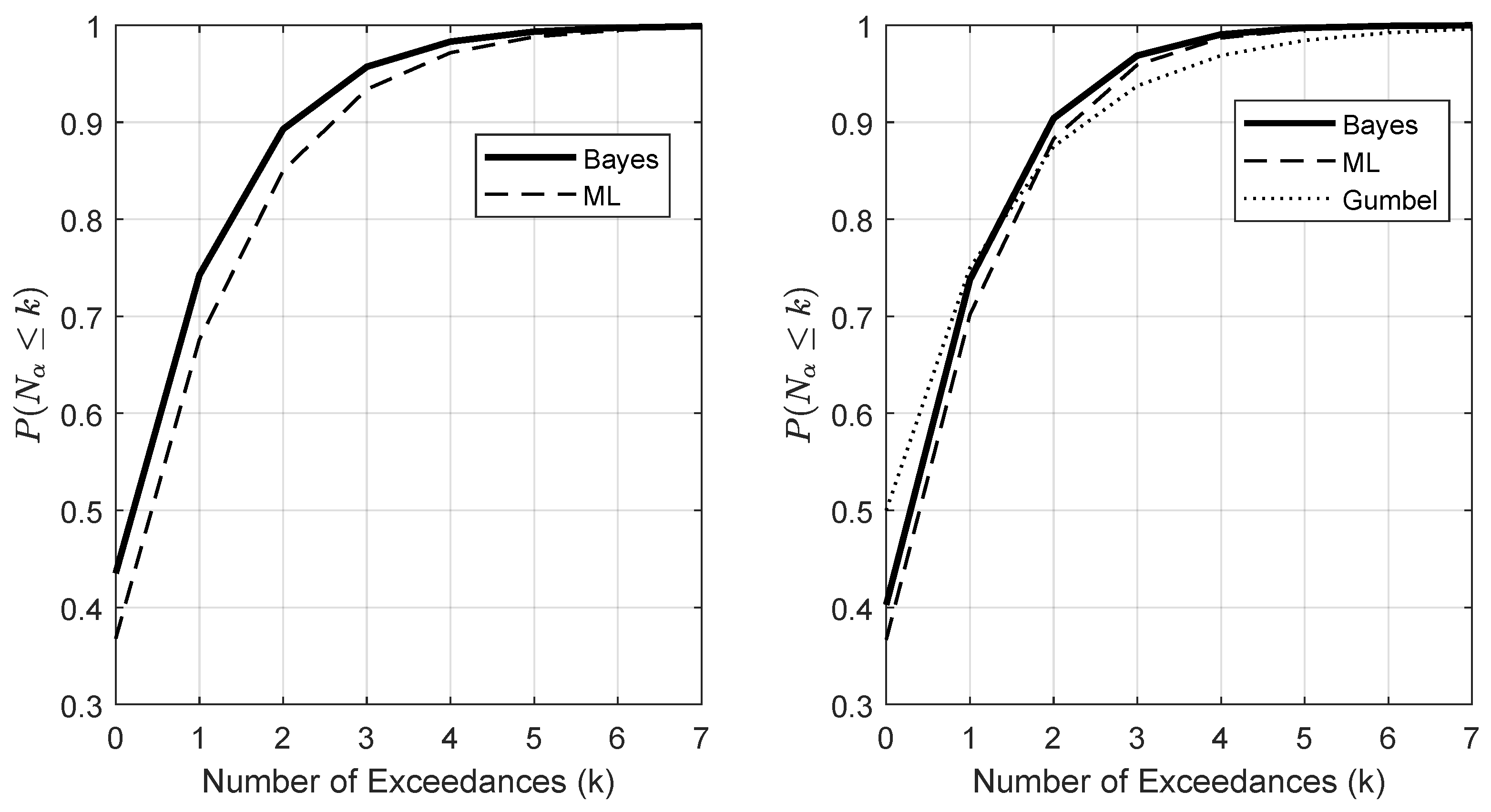
On the left of Figure 2 are the theoretical distributions, $BEG(k;50,100,99\%)$, for both the Bayes and ML quantile estimators with $n=50$ training samples, $N=100$ test samples and $\alpha =99\%$. For all k, the $\mathcal{P}(N_{\alpha }>k)$ is higher for the ML-derived $BEG$ distribution with $E\left[N_{\alpha }\right]=1.22$ and $Var\left[N_{\alpha }\right]=2.11$ compared to the Bayesian-derived $BEG$ distribution with $E\left[N_{\alpha }\right]=1$ and $Var\left[N_{\alpha }\right]=1.46$. We note that for this case, since $n<N$ and $\alpha =1-1/N$, an empirical quantile estimate using the highest-order statistic is not directly applicable.

On the right of Figure 2 are the $BEG(k;100,100,99\%)$ distributions along with the GvS distribution, $w(100,1,100,k)$, of rare exceedances (Gumbel & von Schelling, 1950), which is a distribution-free estimate using, in this case, the first-order statistic for the $\alpha$-quantile since $n=N=1/(1-\alpha )$. While the GvS distribution has mean 1, its variance is 2 compared to the Bayesian-derived $BEG$ distribution which has variance 1.21. The GvS distribution has higher probabilities for a larger number of exceedences, which is not totally surprising given it is a distribution-free, empirical, quantile estimator. The-ML derived $BEG$ distribution results in subpar perfomance with $E\left[N_{\alpha }\right]=1.11$ and $Var\left[N_{\alpha }\right]=1.48$.

2.3. Extending the Exponential Distribution

In general, if Z is from a distribution that can be transformed by a one-to-one transformation to $X=h\left(Z\right)\sim Exp\left(\lambda \right)$, then we can produce quantile estimates from the transformed data and ${\widehat{\eta }}_{\alpha }^Z=h^{-1}(\mathrm{\Psi }\sum h\left(z_i\right))$. Because h is one-to-one, ${\widehat{\eta }}_{\alpha }^Z=h^{-1}\left({\widehat{\eta }}_{\alpha }^X\right)$ or $\mathcal{P}(Z>{\widehat{\eta }}_{\alpha }^Z)=\mathcal{P}(X>{\widehat{\eta }}_{\alpha }^X)$. In addition, since $Z>{\widehat{\eta }}_{\alpha }^Z$ iff $X>{\widehat{\eta }}_{\alpha }^X$, we have $N_{\alpha }^X=N_{\alpha }^Z$ and, therefore, $E\left[N_{\alpha }^X\right]=E\left[N_{\alpha }^Z\right]$. Therefore, our results apply to any distribution that is isomorphic to the exponential distribution and the distribution of exceedances will be invariant.

The MLM estimate of the quantile itself is invariant under the 1-1 RV transformation as long as the transformation does not depend on the parameter. Given $f(x/\lambda )=f(z/\lambda )|dz/dx|$ evaluated at $y=h^{-1}\left(x\right)$, if $|dz/dx|$ is just a scale factor, independent of $\lambda$, then the MLM estimate is ${\widehat{\lambda }}_{ML}=1/\overline{X}=1/\overline{h\left(Z\right)}$ so that

$${\widehat{\eta }}_{\alpha ,ML}^Z=h^{-1}\left(-{\displaystyle \frac{log(1-\alpha )}{n}}\sum h\left(z_i\right)\right)$$

(29)

and the MLM, like the Bayesian method, is invariant under h although, in general, the MLM quantile estimate will no longer be unbiased.

More generally, if Z is a random variable with cdf $F\left(z\right)=1-e^{-\lambda h\left(z\right)}$ with $\lambda >0$, $h\left(z\right)\ge 0$, and h strictly increasing, or $F\left(z\right)=e^{-\lambda h\left(z\right)}$ with h strictly decreasing, and the support is $[u,\infty )$ and h(u) = 0 (or $(u,\infty )$ and ${lim}_{w\to u}h\left(w\right)=0$), then a ZCE quantile estimate is constructed as ${\widehat{\eta }}_{\alpha }^Z=h^{-1}(\mathrm{\Psi }\sum h\left(z_i\right))$ with $\mathrm{\Psi }={(1-\alpha )}^{-1/n}-1$ or $\mathrm{\Psi }={\left(\alpha \right)}^{-1/n}-1$, respectively.

In the first case, we can show that $X=-log(1-F_1\left(Z\right))\sim Exp\left(\lambda \right)$ where $F_1(·)$ is $F(·)$ with $\lambda =1$. In this case, $X=-log(1-(1-e^{-h\left(z\right)}))=h\left(z\right)$ and $dX/dZ=h^{\prime }\left(x\right)$ so by the usual change in variables

$$f_X\left(x\right)={\displaystyle \frac{f_Z\left(z\right)}{|dX/dZ|}}={\displaystyle \frac{\lambda h^{\prime }\left(x\right)e^{-\lambda h\left(h^{-1}\left(x\right)\right)}}{h^{\prime }\left(x\right)}}=\lambda e^{-\lambda x}$$

(30)

and similarly for the second case. An example with numerous applications is the Rayleigh distribution, $f_Z\left(z\right)={\displaystyle \frac{z}{{\sigma }^2}}{e}^{-z^2/2{\sigma }^2}$, where $h\left(Z\right)=Z^2$. Another example is the standard Pareto distribution, with tail-index $1/\lambda$,

$$F\left(z\right)=1-{\left({\displaystyle \frac{z}{u}}\right)}^{-\lambda }=1-e^{-\lambda log(z/u)}z\ge u$$

(31)

so that $h\left(Z\right)=log(Z/u)$ and a ZCE quantile estimate is

$${\widehat{\eta }}_{\alpha }^Z=u{e}^{\mathrm{\Psi }\sum log(z_i/u)}\mathrm{\Psi }={(1-\alpha )}^{-1/n}-1$$

(32)

assuming u is fixed. In the next section, we use this result to model the conditional tail of distributions that have asymptotic Paretian tails such as those in the Fréchet maximum domain of attraction.

It is worth noting that if $Z\sim F\left(Z\right)$ can be transformed to a uniform distribution, $U[0,1]$, then $-log\left(F\right(Z\left)\right)\sim Exp\left(1\right)$, hence a ZCE quantile estimate can be formed. This approach, suggested by (Yu & Ally, 2009), can be used when the parameters of the cdf, F, are known such as if the scale parameter $\lambda =1$.

3. ZCE Quantile Estimation for Paretian Tails

In this section, we extend the results from Section 2 to heavy-tailed distributions, with power-law decay, that are commonly used in financial risk-management. Using standard results from Extreme Value Theory, we model the exceedances above a high threshold as a marked Poisson process with Pareto exceedances and derive the ZCE quantile estimate, and exceedance distribution, using the Bayesian method of marginalizing over the Pareto and Poisson parameters.

3.1. Extreme Value Theory

The theory of extremes is a well-established branch of probability theory and statistical science (S. Coles, 2004; Gumbel, 1958). Consider the maximum, $M_n=max\{X_1,X_2,\cdots ,X_n\}$, of i.i.d. random variables (RVs) with common distribution function (cdf) $X\sim G\left(x\right)$. If the cdf of $M_n\sim G^n\left(x\right)$, properly normalized, converges to a non-degenerate distribution, the Fisher–Tippet–Gnedenko theorem states that it is in the generalized extreme value (GEV) family with tail-index $\xi$ (Embrechts et al., 2003). This distribution has the Jenkinson–von Mises representation,

$$H_{\xi }\left(y\right)=exp(-{(1+\xi y)}^{-1/\xi }),$$

(33)

and we say G is in the maximum domain of attraction of $H_{\xi }$ denoted as $G\in MDA\left(H_{\xi }\right)$. Our interest lies with $\xi >0,y\ge -1/\xi$, resulting in the standard Fréchet distribution which is the limiting class for many underlying heavy-tailed distributions. By the convergence in type theorem, all normalizing sequences converge to the same limit so, more generally, we can state $G\in MDA\left(H_{\xi ,\mu ,\beta }\right)$ with location $\mu$ and scale $\beta$.

The excess distribution, or conditional tail, is defined as $G_u\left(x\right)=\mathcal{P}(X-u\le x|X>u)$ and the Pickands–Balkema–de Haan theorem states that there exists a positive-measurable function $\beta \left(u\right)$ such that

$$\underset{u\to \infty }{lim}\underset{x\ge 0}{sup}|G_u\left(x\right)-G_{\xi ,0,\beta \left(u\right)}\left(x\right)|=0$$

(34)

if and only if $G\in MDA\left(H_{\xi }\right)$ where $G_{\xi ,\mu ,\beta }$ is the generalized Pareto distribution (GPD) with the same tail-index as the GEV (Balkema & de Haan, 1974; Pickands, 1975).

Once again, more generally, if $G\in MDA\left(H_{\xi ,\mu ,\beta }\right)$, the conditional tail distribution, for $x\ge u$, is

$$G_u\left(x\right)=P\left[X<x|X>u\right]\approx 1-{\left[1+{\displaystyle \frac{x-u}{\beta /\xi +u-\mu }}\right]}^{-1/\xi }\sim G_{\xi ,u,\beta +\xi (u-\mu )}.$$

(35)

and a simplifying assumption (Johnston & Djurić, 2020) is that the support of $M_n$ is $[0,\infty )$, or $\mu =\beta /\xi$, and the conditional tail reduces to a standard Pareto,

$$G_{\xi ,u}\left(x\right)=1-{\left({\displaystyle \frac{x}{u}}\right)}^{-1/\xi }x\ge u,$$

(36)

with scale parameter u. In addition to reducing the parameter set, the Pareto RV can be transformed to an exponential distribution which is the basic assumption used for traditional methods of tail index, and a large quantile estimation (Dekkers & de Haan, 1989; Hill, 1975; Pickands, 1975).

Given a high threshold, u, the point process of exceedances converges to a compound Poisson process and is commonly referred to as the ‘Peaks over Threshold’ (POT) model (Leadbetter, 1991). Methods for threshold selection (Northrop et al., 2017) or marginalization of u (Johnston & Djurić, 2021) have been investigated, although often the threshold is set to include a fixed number of high exceedances (Buishand, 1989).

3.2. Data Definition and Solution

The underlying data consist of $\tilde{n}$ “blocks” with the i’th block having length $m_i$ and, to be concrete, we assume each block is a year. The exceedances $\{x_1,\cdots ,x_n\}$ are culled from the data by choosing the threshold u equal to the $(n+1)$’st largest-order statistic. This results in exceedances that are in the top $100\times {\displaystyle \frac{n}{\tilde{n}\overline{m}}}$ percentile with $\overline{m}$ the average number of observations per year. In some fields, such as hydrology, the resulting samples are referred to as the partial duration series, or annual exceedance series when $n=\tilde{n}$. On average, there are ${\displaystyle \frac{n}{\tilde{n}}}$ observations per year and, if $\overline{m}$ is large enough, the POT model is justified.

Since a Pareto RV is isomorphic to an exponential RV, we denote the exceedances as $x_{1:n}=\{ln(x_1/u),\cdots ,ln(x_n/u)\}$, which are i.i.d. and have distribution $F(x/\lambda )\sim$ Exp($\lambda$) with $\lambda =1/\xi$. Furthermore, the number of exceedances are Poisson, Poi(${\lambda }_u$), so that our observations, or training data, $(n,x_{1:n})$, form a marked Poisson process with both parameters, $\lambda$ and ${\lambda }_u$, unknown. Given N future years, we let $y_{1:N_u}$ denote the $N_u$ threshold exceedances of u and $N_{\alpha }$ the number of those exceedances above ${\widehat{\eta }}_{\alpha }$. Typical levels for $\alpha$ range from 99% to an extreme 99.99%. As before, we wish to determine the unconditional distribution of future exceedances of ${\widehat{\eta }}_{\alpha }$ or $\mathcal{P}(N_{\alpha }=k)$ for $k=0,1,\dots N_u$ and, in particular, $E\left[N_{\alpha }\right]$.

Given our u threshold, $N_u$ is unknown but follows a Poisson process with rate parameter ${\lambda }_u$. The maximum likelihood estimate for $E\left[N_u\right]$ would simply be $\widehat{N_u}={\displaystyle \frac{n}{\tilde{n}}}N$ based on a Poisson posterior with $\widehat{{\lambda }_u}={\displaystyle \frac{n}{\tilde{n}}}$. Given the partial duration series, with n samples in $\tilde{n}$ years, the posterior, $\mathcal{P}({\lambda }_u/n)$ is a $\Gamma (n+a,\tilde{n}+b)$ distribution, using a $\Gamma (a,b)$ conjugate prior, and the predictive distribution is therefore a negative binomial

$$N_u\sim \mathrm{NB}\left(n+a,{\displaystyle \frac{\tilde{n}+b}{\tilde{n}+N+b}}\right).$$

(37)

Using a Jeffreys prior, with $a=1/2,b=0$, results in

$$E\left[N_u\right]={\displaystyle \frac{n}{\tilde{n}}}N(1+{\displaystyle \frac{1}{2n}})$$

(38)

and if $n=\tilde{n}>>1$ then $E\left[N_u\right]\approx N$.

Given the results from Section 2.1, we can write the conditional expectation for the number of quantile estimate exceedances as

$$E\left[N_{\alpha }\right|N_u]={\displaystyle \frac{N_u}{{(\mathrm{\Psi }+1)}^n}}$$

(39)

and, since we desire a ZCE quantile estimator with $\mathcal{P}(y>{\widehat{\eta }}_{\alpha ,Bayes})=1-\alpha$, our Bayesian estimate requires

$$\mathrm{\Psi }={\left({\displaystyle \frac{\frac{n}{\tilde{n}}(1+\frac{1}{2n})}{1-\alpha }}\right)}^{1/n}-1$$

(40)

so that the unconditional estimate $E\left[N_{\alpha }\right]=1$ and, as before, $\alpha$ is the annual quantile. We note that if $n=\tilde{n}>>1$, then $\mathrm{\Psi }\approx {\left(1-\alpha \right)}^{-1/n}-1$ as for the unconditional estimate. If $n=\tilde{n}$ but small, then

$$\mathrm{\Psi }\approx {\left({\displaystyle \frac{(1+\frac{1}{2n})}{1-\alpha }}\right)}^{1/n}-1$$

(41)

and ${\widehat{\eta }}_{\alpha }$ is higher than the unconditional estimate to account for the added uncertainty in the number of u exceedances, $N_u$. If $n<\tilde{n}$ but large then

$$\mathrm{\Psi }\approx {\left({\displaystyle \frac{n/\tilde{n}}{1-\alpha }}\right)}^{1/n}-1$$

(42)

and ${\widehat{\eta }}_{\alpha }$ is lower than the unconditional estimate because the threshold u is lower. In effect, we do not need as high of a conditional quantile to achieve the equivalent annual, unconditional, quantile. The ML estimate would result in a similar value of $\mathrm{\Psi }$ as for the unconditional distribution

$${\mathrm{\Psi }}_{ML}={\left({\displaystyle \frac{\frac{n}{\tilde{n}}N}{1-\alpha }}\right)}^{1/n}-1.$$

(43)

The unconditional distribution for exceedance count is

$$P(N_{\alpha }=k)=\sum _{N_u=k}^{N_m}BEG(k;n,N_u,\alpha )\times NB(N_u;n+{\displaystyle \frac{1}{2}},{\displaystyle \frac{\tilde{n}}{\tilde{n}+N}})$$

(44)

where the upper limit is the total number of test samples. In practice, the summation can be truncated and simulation results show that using $N_u=E\left[N_u\right]=N$ does not affect the exceedance distribution significantly.

4. Simulation Results

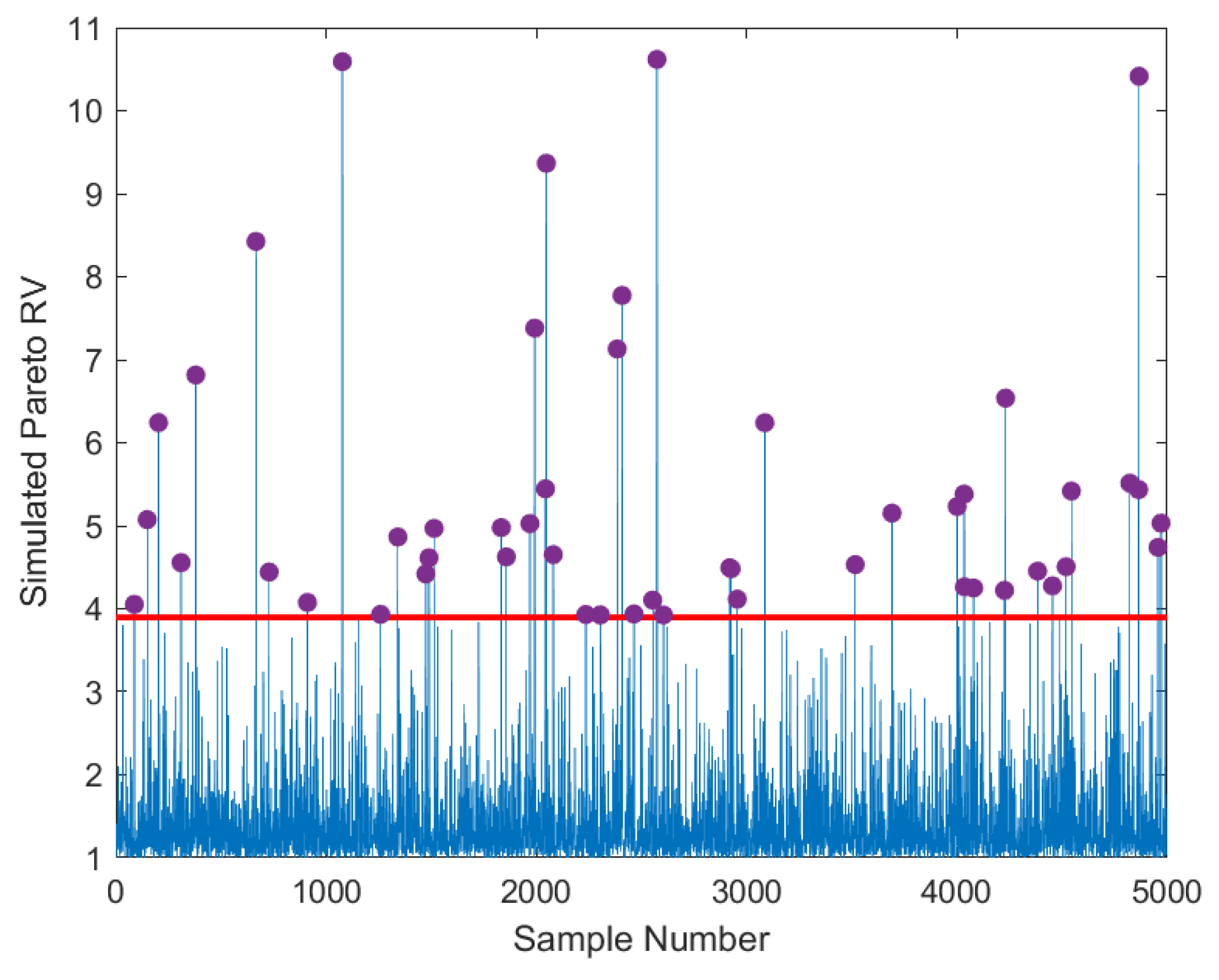
To illustrate the performance of the Bayesian and MLM quantile estimate, we began with a simulation of a standard Pareto RV with tail-index $\xi =0.3$, an example of which is shown in Figure 3. We used $\tilde{n}=50$ with $\overline{m}=100$ samples per year. The threshold u was chosen to select the $n=50$ extreme events highlighted in the Figure. Given the underlying data are Pareto, we might expect the Bayesian method to perform well and, also, we could apply our results directly to all of the data if desired. We assumed N = 100 years and we performed 10,000 runs to gather statistics.

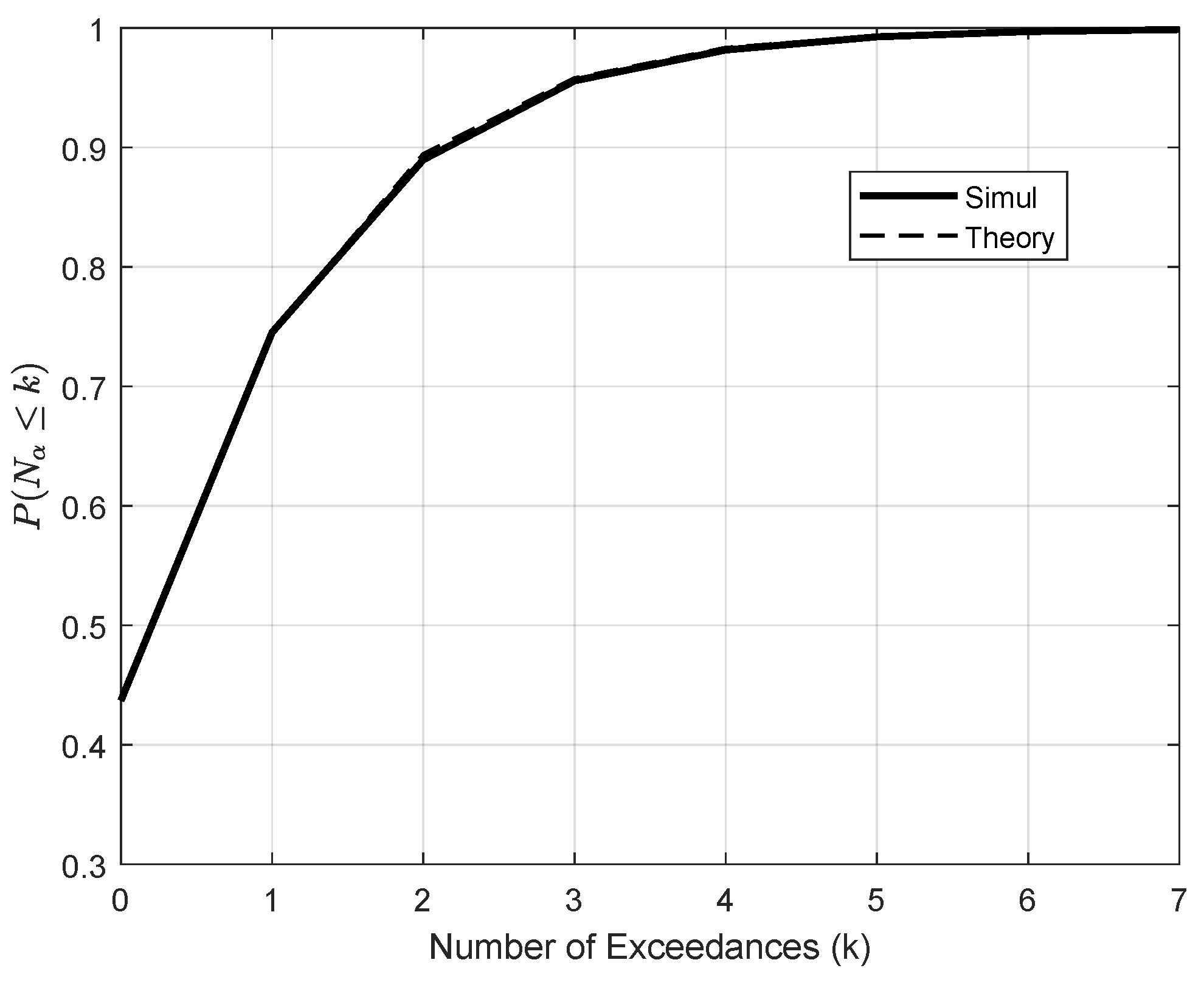
Figure 4 shows the theoretical $BEG(k;50,100,99\%)$ distribution along with the observed frequency distribution from the simulation using the Bayesian quantile estimator. The results agree and, while the expected number of exceedances is one, there is a significant probability of more than one exceedance. In some applications, where an exceedance implies a crititcal failure, this point may be moot, but the exceedance distribution is insightful for risk managers and policy makers to consider. In fact, a more desirable quantile estimator might be to solve for $\mathrm{\Psi }$ in Equation (25) such that $\mathcal{P}(N_{\alpha }=0)$ is a fixed value (e.g., 50%).

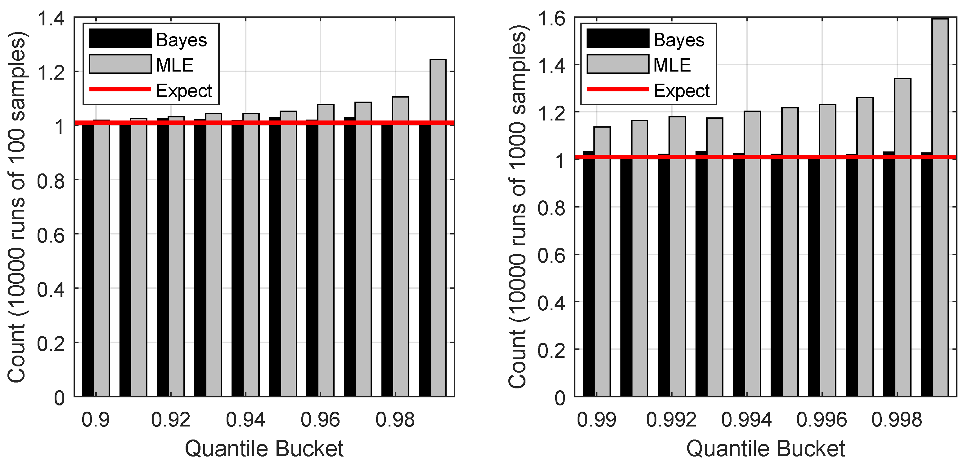
Figure 5 (left) shows the simulation exceedance count divided by the number of simulation runs for the prediction intervals of 1% from 90% to 99% with $N=100$ for both the Bayes and the MLM quantile estimators. The Bayesian estimator performs as advertised with an average number of 1 sample per simulation run which compares the MLM, which underestimates the quantile, in terms of coverage error, resulting in excessive exceedances.

Figure 5 (right) shows the more stressful case with prediction intervals of 0.1% from 99% to 99.9% with $N=1000$. Once again, the Bayesian results in ZCE while the MLM performs rather poorly, particularly at the highest 99.9% quantile. While such a stressful scenario of trying to estimate a 99.9% quantile given only 50 samples may seem unlikely, we note that similar estimates have been required in response to natural disasters (van Dantzig, 1954).

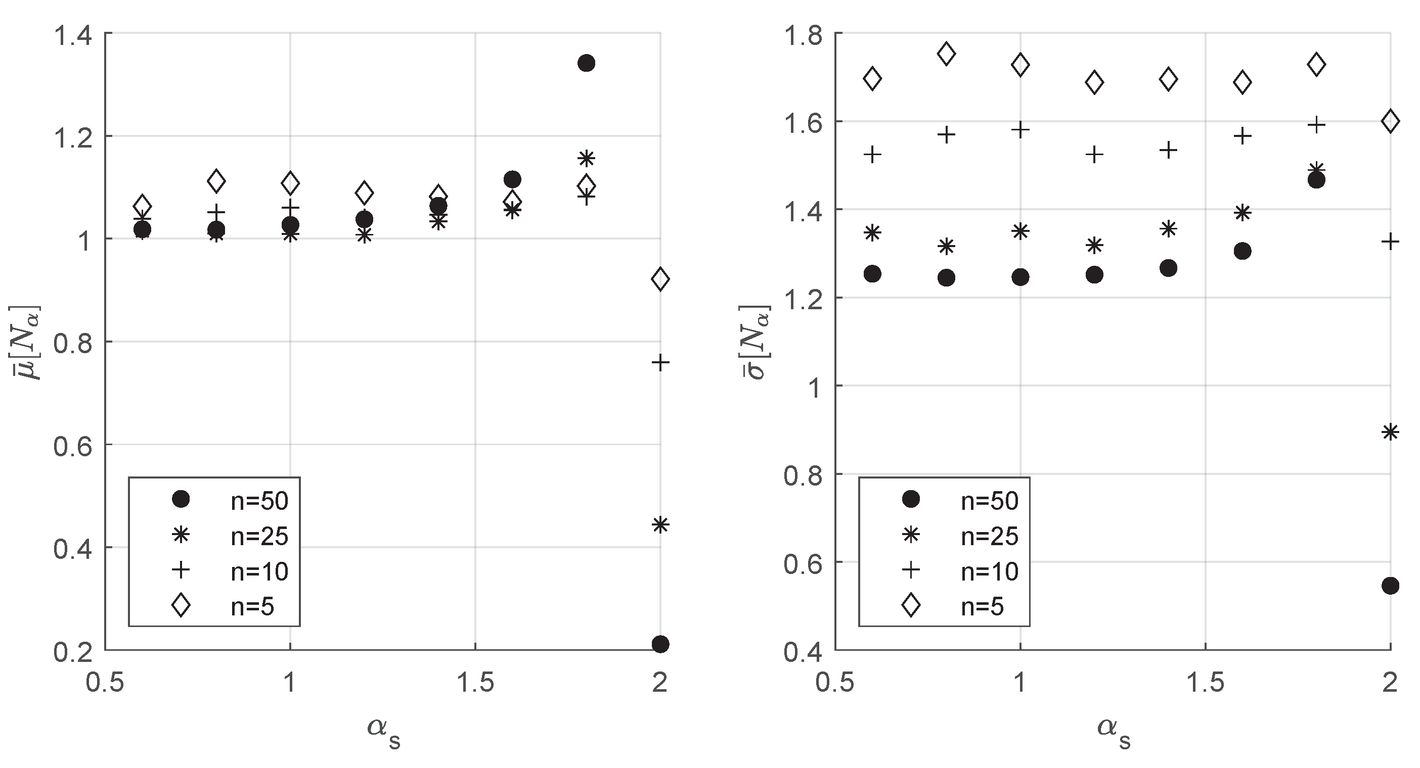
As expected, our method works well when the underlying distribution has a Paretian tail. To explore how the estimator performs when the underlying distribution has an asymptotic Paretian tail, we ran the simulation using a stable ${\alpha }_s$ symmetric (S$\alpha$S) distribution for different values of the characteristic exponent ${\alpha }_s$. We do not necessarily advocate using our method if an S$\alpha$S distribution is appropriate and, in that context, estimating ${\alpha }_s$ and quantiles directly is advised (DuMouchel, 1983). As in our first example, we used $\tilde{n}=50$ with $\overline{m}=100$ samples per year resulting in 5000 total samples. We used N = 100 years with $\alpha =99\%$, and we performed 10,000 runs.

As can be seen in Figure 6, the performance of our quantile estimate is sensitive to the number of tail-samples chosen (n) as ${\alpha }_s\to 2$. This is not surprising, as the inflection point, beyond which a Paritian tail can be deemed appropriate, increases as ${\alpha }_s\to 2$ (Fofack & Nolan, 1999). This results in a need to reduce the number of tail-samples (increase threshold u) to $\approx$0.1% of total samples although this comes with the cost of higher variability unless the total number of samples ($\tilde{n}\overline{m}$) can be increased.

For values of ${\alpha }_s<1.5$, the method performs well for all values of n with $n=50$ or 1% of the total samples resulting in the best performance with the lowest variability. Since ${\alpha }_s<1.5$ implies a heavy-tail with most of the distribution having power-law decay, there is less bias introduced to the quantile estimate. When ${\alpha }_s=2$, a normal distribution not in the Fréchet domain, the sensitivity of the quantile to outliers is evident as is documented in the literature (Weron, 2001).

To further investigate the performance of the Bayesian quantile estimator, we applied it to different underlying distributions with statistics reported in

Table 1. Simulation statistics for the tail-index, $\xi$, and the number of exceedances, $N_{\alpha }$, for various distributions and for different tail-samples (n) with $\tilde{n}\overline{m}$ = 5000, N = 100, and $\alpha =99\%$.

	Exp ($\mu =1$)				Lognormal ($\mu =0$, $\sigma =1$)
	n = 5	n = 10	n = 25	n = 50	n = 5	n = 10	n = 25	n = 50
$\overline{\mu }\left[\xi \right]$	0.13	0.14	0.16	0.18	0.28	0.29	0.32	0.34
$\overline{\sigma }\left[\xi \right]$	0.05	0.04	0.03	0.02	0.12	0.09	0.06	0.04
$\overline{\mu }\left[N_{\alpha }\right]$	0.95	0.78	0.48	0.25	0.98	0.90	0.71	0.53
$\overline{\sigma }\left[N_{\alpha }\right]$	1.67	1.37	0.93	0.60	1.60	1.45	1.12	0.88
$\overline{\mathcal{P}}(N_{\alpha }>1)$	0.21	0.18	0.10	0.04	0.23	0.22	0.17	0.11
	StdPar ($\xi$ = 0.1)				GEV ($\xi$ = 0.5, $\beta$ = 1, $\mu$ = 0)
	n = 5	n = 10	n = 25	n = 50	n = 5	n = 10	n = 25	n = 50
$\overline{\mu }\left[\xi \right]$	0.10	0.10	0.10	0.10	0.52	0.51	0.53	0.54
$\overline{\sigma }\left[\xi \right]$	0.04	0.03	0.02	0.01	0.23	0.16	0.10	0.07
$\overline{\mu }\left[N_{\alpha }\right]$	1.08	1.04	1.03	1.0	1.05	1.03	0.94	0.88
$\overline{\sigma }\left[N_{\alpha }\right]$	1.70	1.53	1.37	1.22	1.70	1.50	1.30	1.14
$\overline{\mathcal{P}}(N_{\alpha }>1)$	0.26	0.25	0.26	0.26	0.25	0.25	0.23	0.23
	StudentT ($\nu =2$)				StudentT ($\nu =10$)
	n = 5	n = 10	n = 25	n = 50	n = 5	n = 10	n = 25	n = 50
$\overline{\mu }\left[\xi \right]$	0.50	0.50	0.50	0.51	0.14	0.15	0.17	0.18
$\overline{\sigma }\left[\xi \right]$	0.23	0.16	0.10	0.07	0.06	0.04	0.03	0.02
$\overline{\mu }\left[N_{\alpha }\right]$	1.08	1.04	1.0	0.95	1.02	0.86	0.64	0.40
$\overline{\sigma }\left[N_{\alpha }\right]$	1.71	1.57	1.34	1.19	1.69	1.39	1.07	0.73
$\overline{\mathcal{P}}(N_{\alpha }>1)$	0.25	0.25	0.25	0.24	0.24	0.20	0.14	0.08

. Similarly to the results when ${\alpha }_s=2$, the estimator is too conservative for thinner, exponential-tailed distribution such as the exponential or lognormal. These distributions, which belong to the Gumbel maximum domain of attraction, require less tail-samples, about 0.1% of total samples, to avoid outlier-bias issues. This may not be that surprising as we are fitting a power-law tail to exponential decay or, effectively, using the wrong tool for the job.

The method works well for the standard Pareto even when the tail index is closer to 0 (i.e., $\xi =0.1$) and also for the GEV, or Fréchet, distribution. We specifically chose $\mu =0\ne \beta /\xi$ so that our condition to simplify the conditional tail to a standard Pareto is violated (see Section 3.1). The variance–bias trade-off is seen as the average number of exceedences declines to 0.88 for 1% sample selection ($n=50$) while the variance in the number of exceedences also declines. Lastly, we show the simulation results for two Student t-distributions. A heavy-tailed version with degrees of freedom, $\nu =2$, and lighter tail with $\nu =10$.

5. Discussion

In this research, we have derived a Bayesian quantile estimator and the distribution of exceedances that can be applied to distributions that are isomorphic to the exponential distribution or whose tail exhibits power-law decay. We show the derived quantile estimate has zero coverage error implying the probability of exceedance, from a frequentist perspective, agrees with the desired quantile. This is a critical requirement for proper risk management and insures the usefulness of our approach, particularly for small sample sizes. Small sample size analysis is increasingly important given the inherent non-stationarity of financial markets.

In addition to deriving the ZCE quantile estimate, we derive an analytic expression for the distribution of the number of exceedences. This is a new result and important in analyzing the risk of multiple extreme events, potentially leading to significant losses and financial impairment. Given traditional methods underestimate this risk, our novel approach is a clear benefit for analyzing financial markets and will allow financial risk-managers to make more reliable risk assessments.

The theoretical performance of our approach exceeds the traditional maximum likelihood method and simulation results prove the efficacy of our methodology. Our method can be applied to a variety of underlying heavy-tailed distributions, in the Fréchet domain, that are typically encountered in financial market data. For example, historical analysis of stock market returns indicates the underlying process to be in the Fréchet domain with tail-index values in the 0.25 to 0.5 range. This implies our method would produce superior VaR or expected shortfall analyses. While the usual trade-off between variance and bias exists, for tails that are not strictly Pareto, the Bayesian method produces results that are an improved alternative to traditional risk-management metrics.

References

1. Bairamov, I. G. (1996). Some distribution free properties of statistics based on record values and characterizations of the distributions through records. Journal of Applied Statistical Science, 5(1), 17–25. [Google Scholar]
2. Balkema, A., & de Haan, L. (1974). Residual life time at great age. Annals of Probability, 2(5), 792–804. [Google Scholar] [CrossRef]
3. Broadwater, J. B., & Chellappa, R. (2010). Adaptive threshold estimation via extreme value theory. IEEE Transactions on Signal Processing, 58(2), 490–500. [Google Scholar] [CrossRef]
4. Buishand, T. A. (1989). The partial duration series method with a fixed number of peaks. Journal of Hydrology, 109(1–2), 1–9. [Google Scholar] [CrossRef]
5. Coles, S. (2004). An introduction to statistical modeling of extreme values. Springer. [Google Scholar]
6. Coles, S. G., & Dixon, M. J. (1999). Likelihood-based inference for extreme value models. Extremes, 2(1), 5–23. [Google Scholar] [CrossRef]
7. Coles, S. G., & Powell, E. A. (1996). Bayesian methods in extreme value modelling: A review and new developments. International Statistical Review, 64(1), 119–136. [Google Scholar] [CrossRef]
8. Datta, G. S., Mukerjee, R., Ghosh, M., & Sweeting, T. J. (2000). Bayesian prediction with approximate frequentist validity. The Annals of Statistics, 28(5), 1414–1426. [Google Scholar] [CrossRef]
9. Dekkers, A. L. M., & de Haan, L. (1989). On the estimation of the extreme-value index and large quantile estimation. Annals of Statistics, 17(4), 1795–1832. [Google Scholar] [CrossRef]
10. DuMouchel, W. H. (1983). Estimating the stable index α in order to measure tail thickness: A critique. The Annals of Statistics, 11(4), 1019–1031. [Google Scholar] [CrossRef]
11. Embrechts, P., Kluppelberg, C., & Mikosch, T. (2003). Modelling extremal events. Springer. [Google Scholar]
12. Fofack, H., & Nolan, J. P. (1999). Tail behavior, modes and other characteristics of stable distributions. Extremes, 2, 39–58. [Google Scholar] [CrossRef]
13. Gumbel, E. J. (1958). Statistics of extremes. Columbia University Press. [Google Scholar]
14. Gumbel, E. J., & von Schelling, H. (1950). The distribution of the number of exceedances. The Annals of Mathematical Statistics, 21(2), 247–262. [Google Scholar] [CrossRef]
15. Hall, P., & Rieck, A. (2001). Improving coverage accuracy of non-parametric prediction intervals. Journal of the Royal Statistical Society B, 63(4), 717–725. [Google Scholar] [CrossRef]
16. Hill, B. M. (1975). A simple general approach to inference about the tail of a distribution. Annals of Statistics, 3(5), 1163–1174. [Google Scholar] [CrossRef]
17. Hosking, J. R. M., & Wallis, J. R. (1987). Parameter and quantile estimation for the generalized Pareto distribution. Technometrics, 29(3), 339–349. [Google Scholar] [CrossRef]
18. Johnston, D. E., & Djurić, P. M. (2011). The science behind risk management: A signal processing perspective. IEEE Signal Processing Magazine, 28(5), 26–36. [Google Scholar]
19. Johnston, D. E., & Djurić, P. M. (2020, May 4–8). A recursive Bayesian solution for the excess over threshold distribution with stochastic parameters. ICASSP 2020, Barcelona, Spain. [Google Scholar]
20. Johnston, D. E., & Djurić, P. M. (2021, June 6–11). Baysian estimation of a tail-index with marginalized threshold. ICASSP 2021 (pp. 5569–5573), Toronto, ON, Canada. [Google Scholar]
21. Leadbetter, M. R. (1991). On a basis for ‘Peaks over Threshold’ modeling. Statistics and Probability Letters, 12(4), 357–362. [Google Scholar] [CrossRef]
22. McNeil, A., Frey, R., & Embrechts, P. (2005). Quantitative risk management. Princeton University Press. [Google Scholar]
23. Nerantzaki, S. D., & Papalexiou, S. M. (2022). Assessing extremes in hydroclimatology: A review on probabilistic methods. Journal of Hydrology, 605, 1–20. [Google Scholar] [CrossRef]
24. Northrop, P. J., Attalides, N., & Jonathan, P. (2017). Cross-validatory extreme value threshold selection and uncertainty with application to ocean storm severity. Journal of the Royal Statistical Society: Applied Statistics, 66(1), 93–120. [Google Scholar] [CrossRef]
25. Pickands, J. (1975). Statistical inference using extreme order statistics. Annals of Statistics, 3(1), 119–131. [Google Scholar]
26. Resnick, S. I., & Rootzeń, H. (2000). Self-similar communication models and very heavy tails. Annals of Applied Probability, 10(3), 753–778. [Google Scholar] [CrossRef]
27. Roberts, S. J. (2000). Extreme value statistics for novelty detection in biomedical data processing. IEE Proceedings-Science, Measurement and Technology, 147(6), 363–367. [Google Scholar]
28. Shenoy, S., & Gorinevsky, D. (2015). Estimating long tail models for risk trends. IEEE Signal Processing Letters, 22(7), 968–972. [Google Scholar] [CrossRef]
29. Smith, R. L. (1987). Estimating tails of probability distributions. The Annals of Statistics, 15(3), 1174–1207. [Google Scholar] [CrossRef]
30. van Dantzig, D. (1954, September 2–9). Mathematical problems raised by the flood disaster of 1953. International Congress of Mathematicians (pp. 218–239), Amsterdam, Denmark. [Google Scholar]
31. Weron, R. (2001). Levy-stable distributions revisited: Tail index > 2 does not exclude the Levy-stable regime. International Journal of Modern Physics, 12(2), 209–223. [Google Scholar] [CrossRef]
32. Wesolowski, J., & Ahsanullah, M. (1998). Distributional properties of exceedance statistics. Annals of the Institute of Statistical Mathematics, 50(3), 543–565. [Google Scholar] [CrossRef]
33. Yu, K., & Ally, A. (2009). Improving prediction intervals: Some elementary methods. The American Statistician, 63(1), 17–19. [Google Scholar] [CrossRef]
34. Yu, K., & Moyeed, R. A. (2001). Bayesian quantile regression. Statistics and Probability Letters, 54(4), 437–447. [Google Scholar]
Figure 1. E [ N α ] versus n for MLM with N = 1 / ( 1 α ) and α = 99 % , 99.9 % , 99.99 % .
Jrfm 18 00659 g001
Figure 2. B E G ( k ; 50 , 100 , 99 % ) , left, and B E G ( k ; 100 , 100 , 99 % ) , right, along with GvS: w ( 100 , 1 , 100 , k ) exceedance distributions.
Jrfm 18 00659 g002
Figure 3. Simulated Pareto RV samples (lines) and threshold exceedances (dots) with ξ = 0.3 , n = n ˜ = 50 , m ¯ = 100 .
Jrfm 18 00659 g003
Figure 4. Theoretical B E G ( k ; 50 , 100 , 99 % ) and simulation frequency distribution for Bayesian quantile estimator.
Jrfm 18 00659 g004
Figure 5. Normalized simulation exceedance count for 1% prediction intervals with n = 50 and N = 100 (left) and 0.1% prediction intervals with n = 50 and N = 1000 (right).
Jrfm 18 00659 g005
Figure 6. Simulation sample mean (left) and standard deviation (right) of the number of exceedances ( N α ) as a function of S α S characteristic exponent α s for different tail-samples (n) with n ˜ m ¯ = 5000, N = 100, and α = 99 % .
Jrfm 18 00659 g006