Systemic Risk Modeling with Expectile Regression Neural Network and Modified LASSO

Abstract

Traditional risk models often fail to capture extreme losses in interconnected global stock markets. This study introduces a novel approach, Expectile Regression Neural Network with Modified LASSO regularization (ERNN-mLASSO), to model nonlinear systemic risk. By analyzing five major stock indices (JKSE, GSPC, GDAXI, FTSE, N225), we identify distinct market roles: developed markets, such as the GSPC, act as risk spreaders, while emerging markets, like the JKSE, act as risk takers. Our network systemic risk index, SNRI, accurately captures systemic shocks during the COVID-19 crisis. More importantly, the model projects increasing global financial fragility through 2025, providing an early warning signal for policymakers and risk managers of potential future instability.

1. Introduction

The rapid development of technology and digitalization has transformed the global stock market into an integrated ecosystem. Capital flows can shift rapidly from one stock market to another, creating a complex network where the stability of one market depends on the conditions of others (Pagliaro, 2025). Research by Allen and Gale (2000) has long demonstrated how interconnectedness between banks can function as contagion channels, a concept now proving relevant on a global scale, as observed in stock markets (Billio et al., 2012). This reality poses a crucial challenge: how to determine whether the stability of one stock market directly impacts the stability of other stock markets, a phenomenon known as systemic risk (Lai & Hu, 2021). Systemic risk is defined as the potential for a local shock in a major financial center or large-cap stock market, such as the S&P 500, to trigger a chain reaction that destabilizes global markets (McClellan, 2025).

To address these challenges, this study proposes a novel nonlinear modeling approach to quantify systemic risk in financial data, called Expectile Regression Neural Network with Modified LASSO Regularization (ERNN-mLASSO). Unlike traditional quantile-based metrics such as Value-at-Risk (VaR) (Marumo & Li, 2024), which tend to underestimate the magnitude of extreme losses (Ahmed & Rura, 2024; Chen & Fan, 2022), our approach leverages expectiles, which are inherently more sensitive to the magnitude of losses in the tails of the distribution (Saux & Maillard, 2023; Waltrup et al., 2015). We combine the statistical advantages of expectiles with the flexibility of neural networks to model complex nonlinear relationships between markets (Jiang et al., 2017; Lin et al., 2022) and augment them with mLASSO regularization to improve predictive accuracy and model efficiency. Using this framework, we estimate individual risk (EVaR) and conditional risk (TERES), which are then used to calculate three complementary systemic risk indicators: the Systemic Fragility Index (SFI), the Systemic Hazard Index (SHI), and the Systemic Network Risk Index (SNRI) (Keilbar & Wang, 2022; Lee et al., 2013; Naeem et al., 2025).

Our empirical analysis of five major global stock indices (JKSE, GSPC, GDAXI, FTSE, and N225) from 2011 to 2025 yields several key findings. First, our results consistently show that large-cap and developed markets, such as the GSPC (S&P 500) and GDAXI (DAX), tend to act as risk spreaders. Shocks originating in these markets have a high capacity to propagate throughout the system, especially during periods of crisis. In contrast, smaller emerging markets, such as the Jakarta Composite Index (JKSE), are more susceptible to contagion and act as risk takers. This finding aligns with the spillover index framework popularized by Diebold and Yilmaz (2012), which measures the direction and intensity of shocks across markets. The second most significant finding relates to the overall network risk dynamics captured by the SNRI. Our SNRI effectively identified a sharp spike in systemic risk during the COVID-19 crisis in early 2020. More worryingly, our model signals a potential even higher increase in systemic risk through 2025, underscoring the growing fragility of the global financial network. This finding highlights the importance of ongoing monitoring, as past crises have taught us that failure to understand and measure these risk transmission dynamics can have fatal consequences, not only for investors but also for the real economy (Acharya et al., 2017; Narayan & Kumar, 2024).

This research positions itself at the intersection of traditional systemic risk modeling literature and machine learning-based ones. While classical econometric models such as multivariate GARCH models are effective in analyzing linear volatility spillovers (Bagirov & Mateus, 2025), they often fail to capture crucial nonlinear contagion dynamics during crises. To address this, machine learning approaches such as neural network quantile regression have emerged as a powerful alternative (Keilbar & Wang, 2022). However, our research offers two key innovations. First, unlike quantile-based approaches, we adopt an expectile framework that is more sensitive to loss magnitudes, and we advance existing linear expectile models (Zhang et al., 2024) by integrating neural network architectures to capture complex nonlinearities. Second, unlike studies focusing on single markets (Kamah & Riti, 2024), we provide a global comparative analysis, allowing us to map the dynamic roles of markets as risk ‘takers’ and ‘spreaders’ within international financial networks.

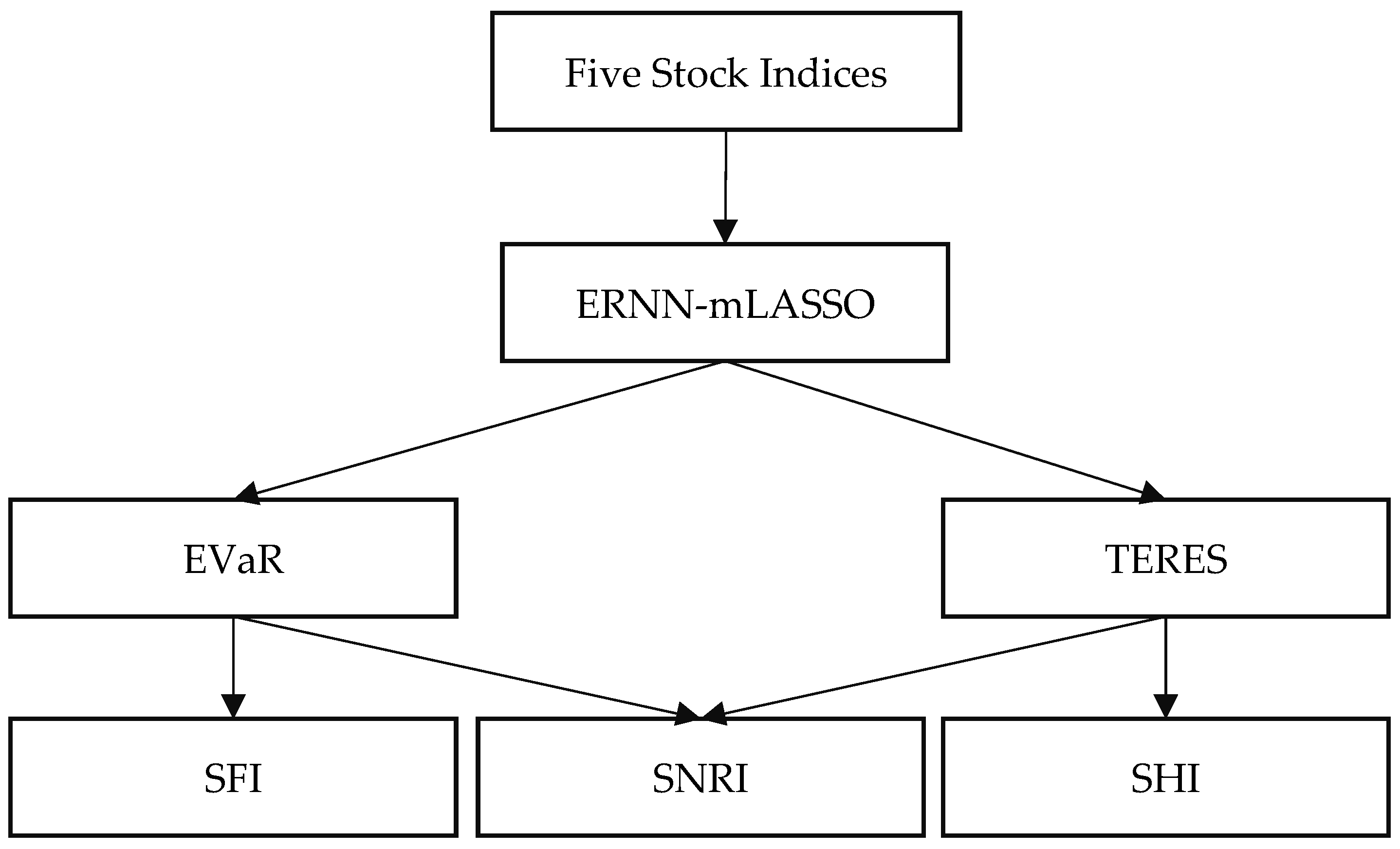
This study makes several key contributions to the literature. First, we propose a new integrated methodology, ERNN-mLASSO, for modeling systemic risk. This novelty lies in its more robust statistical foundation, which utilizes expectiles (Syuhada et al., 2023; Di Bernardino et al., 2024; Yamashita, 2025), and its ability to capture complex nonlinearities often overlooked by traditional linear econometric models (Hong, 2022; Patton, 2006). Second, we provide detailed empirical evidence on the dynamic role of various stock markets—both as risk disseminators and recipients—in the global risk architecture. Unlike studies that focus solely on individual risks (Iqbal et al., 2023), our analysis explicitly maps interconnectedness and contagion pathways. Thus, this research offers a more accurate and relevant perspective for risk management in modern stock markets. To provide a concise visual summary and an intuitive overview of the main contributions of this research, Figure 1 presents the structural flow of the ERNN-mLASSO model, which shows how five global stock indices are processed to produce expectation-based risk measures (EVaR and TERES), which are then carefully used to construct systemic risk indicators (SFI, SHI, and SNRI).

The remainder of this article is structured as follows. Section 2 explains the methodological framework in detail. Section 3 presents the experimental design and simulation results to validate the model. Section 4 discusses empirical application to stock market index data, followed by an in-depth discussion of the results. Finally, Section 5 summarizes the main findings and their implications.

2. Methods

2.1. Expectile Regression

Although Quantile Regression (QR) has a strong intuitive appeal in the development of regression models, Newey and Powell (1987) pointed out three shortcomings of this model, including non-differentiability, inefficiency for Gaussian-like error distributions, and difficulty in calculating the covariance matrix. Therefore, Newey and Powell (1987) proposed Expectile Regression (ER), which uses an asymmetric L2-norm loss function, as an alternative for analyzing the complete conditional response distribution. ER is developed by generalizing mean regression using an asymmetric loss function, resulting in a model that is robust to outliers. In other words, ER is often used when the assumption of a normal distribution fails or when heteroscedasticity of variance is present.

Consider the variables $\left\{\left(x_t,y_t\right),t=1,2,\dots ,T\right\}$, where $x_t$ and $y_t$ respectively denote the predictor and response variables of the ER model, and the ER model parameter vector is expressed as $\beta \left(\tau \right)={\left({\beta }_0\left(\tau \right),{\beta }_1\left(\tau \right),\dots ,{\beta }_p\left(\tau \right)\right)}^T$. The ER model estimator can be obtained in the form of a vector that minimizes the following Asymmetric Least Squares (ALS) loss function (Liao et al., 2019):

$$L\left(\beta \left(\tau \right)\right)={\displaystyle \frac{1}{T}}{\displaystyle \sum _{t=1}^T{\rho }_{\tau }^E\left(y_t-x_t^T\beta \left(\tau \right)\right)},$$

(1)

where $\beta \left(\tau \right)\in {ℝ}^{p+1}$ for a value of $\tau \in \left(0,1\right)$ and ${\rho }_{\tau }^E\left(\cdot \right)$ is a convex loss function which is expressed as:

$${\rho }_{\tau }^E\left(\epsilon \right)=\left\{\begin{array}{c}\hfill \left(1-\tau \right){\epsilon }^2,\epsilon <0\\ \hfill \tau {\epsilon }^2,\epsilon \ge 0\end{array}\right..$$

(2)

In Equation (1), if $\tau$ is 0.5 or 50%, it will be Ordinary Least Square (OLS), so the ER model loss function is considered a generalization of the mean regression. An interesting property of ER is that the ER estimator relies on the entire data distribution, while the QR estimator only relies on the percentiles of the estimated tail distribution. Therefore, the ER estimator contains additional information about the magnitude of the tail distribution and reflects the actual value more accurately.

2.2. Expectile Regression Neural Network

There has been relatively little development of ER models that accommodate nonlinear relationships within the context of nonparametric methods, particularly with Neural Network (NN)-based machine learning. In the same discussion, Jiang et al. (2017) were inspired by the Quantile Regression Neural Network (QRNN) model (Taylor, 2000), and they developed a nonparametric nonlinear regression model, later named the Expectile Regression Neural Network (ERNN), by adding an NN structure to the ER approach. The ERNN model has several advantages over typical regression models. First, because it uses the ALS loss function, the ERNN model can be easily estimated using standard gradient-based optimization algorithms and directly generates the conditional expectile function. This approach is superior to the QRNN model because it relies on the Asymmetric Least Absolute (ALA) loss function, which is not differentiable. Therefore, the QRNN model cannot be estimated using standard gradient-based optimization algorithms until the ALA loss function is approximated using the Huber approximation function as described by Cannon (2011). Second, the ERNN model is flexible enough to explore the potential nonlinear effects of using predictor variables on the expectile of a response variable without specifying a specific nonlinear functional form. Third, the ERNN model is capable of directly generating conditional expectile functions that describe the complete distribution of the response variable depending on the information in the predictor variables (Jiang et al., 2017).

Consider the variables $\left\{\left(x_t,y_t\right),t=1,2,\dots ,T\right\}$, where $x_t$ and $y_t$ respectively denote the predictor and response variables of the ERNN model, which refers to Equation (1). In the ERNN model, the possibility of a nonlinear relationship between $x_t$ and $y_t$ is explored using a three-layer NN structure called a model consisting of input, hidden, and output layers, as shown in Figure 2. The ERNN model differs from the general NN model in two aspects. First, the output of ERNN is the conditional expectile of $y_t$ at a given $\tau$ denoted $E\left(y_t;\tau \right)$. Such estimation can provide a more complete picture of the statistical domain of $y_t$ by considering different $\tau$ values. Second, all parameters, including weights and biases, depend on $\tau$ which implies that the ERNN model is capable of investigating heterogeneous relationships between predictor variables and response variables across specific $\tau$ values (Jiang et al., 2017).

Based on Figure 2, in general, the ERNN model can be expressed as (Jiang et al., 2017):

$$\begin{array}{c}E\left(y_t;\tau \right)=f^{\left(O\right)}\left({\displaystyle \sum _{j=1}^J{v}_j^{\left(O\right)}\left(\tau \right)g_{j,t}\left(\tau \right)+b^{\left(O\right)}\left(\tau \right)}\right)\\ g_{j,t}\left(\tau \right)=f^{\left(H\right)}\left({\displaystyle \sum _{d=1}^p{v}_{d,j}^{\left(H\right)}{x}_{d,t}}+b_j^{\left(H\right)}\left(\tau \right)\right)\end{array}.$$

(3)

The ERNN model is not only flexible in investigating the nonlinear effects of individual predictor variables, but it can also explore all types of interactions between predictor variables. Thus, it is capable of uncovering complex nonlinear relationships by applying the NN model structure. The parameters in the ERNN model are estimated using an empirical loss function with the ALS approach as follows:

$$L\left({\psi }_{\tau }\right)={\displaystyle \frac{1}{T}}{\displaystyle \sum _{t=1}^T{\rho }_{\tau }^E\left(y_t-E\left(y_t;\tau \right)\right)}.$$

(4)

Next, the parameters of the ERNN model are expressed in vectors as ${\psi }_{\tau }={\left({\left(v^{\left(O\right)}\left(\tau \right)\right)}^T,\left(b^{\left(O\right)}\left(\tau \right)\right),{\left(Vec\left(V^{\left(H\right)}\left(\tau \right)\right)\right)}^T,{\left(b^{\left(H\right)}\left(\tau \right)\right)}^T\right)}^T$. The empirical loss function is differentiable at each $\tau$ value and is convex. Therefore, the ERNN model parameters can be estimated using a standard gradient-based nonlinear optimization algorithm and obtain a unique optimal solution as follows:

$${\widehat{\psi }}_{\tau }=\underset{{\psi }_{\tau }}{\arg \min }\left\{L\left({\psi }_{\tau }\right)\right\},$$

(5)

which can then be optimized using several methods, such as the quasi-Newton method.

In the ERNN model in this study, the number $p$ of predictor variables in the input layer and the number $J$ of hidden layer nodes determine the overall model complexity. Models with complex structures can lead to overfitting. Therefore, we added a modified LASSO (mLASSO) penalty to the ERNN model’s loss function, obtaining the following new empirical loss function:

$$L\left({\psi }_{\tau }|\lambda ,J\right)=L\left({\psi }_{\tau }\right)+\lambda \left({‖\left(v^{\left(O\right)}\left(\tau \right)\right)‖}_1+{‖\left(V^{\left(H\right)}\left(\tau \right)\right)‖}_1\right),$$

(6)

where $\lambda$ is a positive Lagrange multiplier parameter determined through grid search optimization.

In empirical applications of the ERNN model, $p$ is usually fixed because the predictor variables are often given in advance. However, the number of ERNN model parameters, namely, the accumulation of the contents of the $V^{\left(H\right)}\left(\tau \right)$ parameter matrix $\left(\#V^{\left(H\right)}\right)$ and the $v^{\left(O\right)}\left(\tau \right)$ parameter vector $\left(\#v^{\left(O\right)}\right)$, which always depends on the determination of the $\lambda$ and $J$ values, plays an important role in generating model estimates and predictions. In statistics, the Akaike Information Criterion (AIC) is a criterion used to select the best statistical model among several candidate models. The AIC balances between the model’s goodness of fit in explaining the data (goodness of fit) and the model’s complexity (number of parameters). The smaller the AIC value, the better the model is considered in terms of the balance between accuracy and simplicity. To find the optimal combination of $\lambda$ and $J$, the AIC measure is formulated as follows:

$$\mathrm{AIC}\left(\lambda ,J\right)=\log \left(L\left({\psi }_{\tau }|\lambda ,J\right)\right)+2\left(\#v^{\left(O\right)}+\#V^{\left(H\right)}+J+1\right),$$

(7)

where $\#v^{\left(O\right)}$ and $\#V^{\left(H\right)}$ denote the number of elements of the parameter vector (weights) in the hidden-output layer and the number of elements of the parameter matrix (weights) in the input-hidden layer in the model (which are not zero), respectively. The optimal values of $\lambda$ and $J$ were determined by selecting the model with the smallest AIC value. The $\lambda$ and $J$ value scenarios were set using a grid search optimization scheme.

2.3. Risk Measurements

Basically, the quantile approach is more commonly used in multivariate risk modeling, both for linear approaches, such as Quantile Vector Autoregressive (QVAR) (Chavleishvili & Manganelli, 2024), and nonlinear approaches, such as Quantile Regression Neural Networks (QRNN) (Naeem et al., 2022). Our choice to adopt an expectile-based framework was a deliberate methodological decision, considering several limitations and shortcomings of the quantile approach. The primary reason is that expectiles are inherently more sensitive to the actual magnitude of losses in the tails of the distribution, not just their probabilities, which are more relevant for measuring the impact of systemic shocks. Furthermore, from a computational perspective, the differentiable quadratic loss function of expectiles is naturally more suitable for the gradient-based optimization algorithm used to train our neural network, compared to the non-differentiable absolute loss function of quantiles. Therefore, the expectile approach was chosen not because it is inferior to the quantile approach, but because it is theoretically and computationally aligned with our goal of modeling systemic risk severity in a complex nonlinear architecture.

In this study, the risk measures used are Expectile-based Value at Risk (EVaR) (Syuhada et al., 2023) and Tail Event Risk Expectile Shortfall (TERES) (Mihoci et al., 2021), rather than the more commonly used Value at Risk (VaR) and Conditional Value at Risk (CoVaR) (Azmi et al., 2022). This choice is based on several methodological considerations. First, VaR has limitations because it only provides information on specific quantiles of the loss distribution and is often incoherent, thus underrepresenting the true level of risk at the tail of the distribution. CoVaR, which was developed to measure risk interconnectedness between entities, also relies on the quantile concept and therefore faces similar limitations (Ullah, 2024).

As an alternative, EVaR uses an expectile approach, which is more flexible and can capture risk information in the loss distribution more finely than VaR. Expectile is coherent and able to integrate sensitivity to changes in the loss distribution, thus providing a more informative risk measure. Meanwhile, TERES was developed to evaluate the risk impact of extreme events at the tail of the distribution, thus more accurately depicting systemic interconnectedness between entities than CoVaR. Thus, the use of EVaR and TERES in this study is expected to provide a more comprehensive understanding of extreme risks and systemic linkages compared to conventional measures such as VaR and CoVaR.

2.3.1. Expectile-Based Value at Risk

Simply put, EVaR can be viewed as the predicted result of an Expectile Regression (ER) model at a certain expectile level, $\tau$ (Syuhada et al., 2023). Thus, EVaR is an extension of the VaR concept, but based on an expectile regression framework. The mathematical formulation of EVaR can be written as follows:

$${\widehat{EVaR}}_{\tau ,t}=x_t^T\widehat{\beta }\left(\tau \right),$$

(8)

where $\widehat{\beta }\left(\tau \right)$ is an estimator of the ER model parameters at the $\tau$ level. The parameter estimates are determined by solving the following optimization problem:

$$\widehat{\beta }\left(\tau \right)=\underset{\beta \left(\tau \right)}{\arg \min }\left\{{\displaystyle \frac{1}{T}}{\displaystyle \sum _{t=1}^T{\rho }_{\tau }^E\left(y_t-x_t^T\beta \left(\tau \right)\right)}\right\}.$$

(9)

2.3.2. Tail Event Risk Expectile Shortfall

The TERES concept was first introduced by Mihoci et al. (2021) as an extension of the Expected Shortfall measure based on an expectile regression framework. This approach was developed to overcome the limitations of quantile-based risk measures by utilizing an asymmetric loss function derived from the squared loss. This results in a smoother and more efficient estimate of tail risk. Calculating the TERES value requires the use of an expectile basis. If the TERES is estimated using an ERNN (Expectile Regression Neural Network) model, the obtained value indirectly represents the model’s predicted output. In other words, the TERES for an index can be interpreted as the predicted value of the ERNN model, where the predictor used is the EVaR of another relevant index.

Mathematically, the TERES value for an index (for example, A) can be expressed using a specific formula, as shown in the following equation:

$$\begin{array}{c}{\widehat{TERES}}_t^A\left(\tau \right)=f^{\left(O\right)}\left({\displaystyle \sum _{j=1}^J{\widehat{v}}_j^{\left(O\right)}\left(\tau \right){\widehat{g}}_{j,t}\left(\tau \right)+{\widehat{b}}^{\left(O\right)}\left(\tau \right)}\right)\\ \hspace{1em}\hspace{1em} {\widehat{g}}_{j,t}\left(\tau \right)=f^{\left(H\right)}\left({\displaystyle \sum _{d\ne A}{\widehat{v}}_{d,j}^{\left(H\right)}\left(\tau \right){\widehat{EVaR}}_{\tau ,t}^d+{\widehat{b}}_j^{\left(H\right)}\left(\tau \right)}\right)\end{array},$$

(10)

where ${\widehat{EVaR}}_{\tau ,t}^d$ denotes the estimated EVaR value of an index $d$.

2.4. Systemic Risk Index

The Systemic Risk Index is a measurement framework used to assess the level of systemic risk in financial markets. Systemic risk itself refers to a situation where shocks in one part of the market spread to other parts and have the potential to disrupt overall financial stability. To provide a comprehensive picture, the SRI is constructed in three interrelated measures: the Systemic Fragility Index (SFI), the Systemic Hazard Index (SHI), and the Systemic Network Risk Index (SNRI) (Keilbar & Wang, 2022). The SFI emphasizes market vulnerability to risk shocks. The SHI measures the degree of crisis-based risk transmission from one index to another. The SNRI assesses overall systemic risk by considering the interconnectedness of financial entities through spillover mechanisms. These three measures highlight different aspects of systemic risk: index vulnerability, the degree of risk transmission, and the interconnectedness of the financial risk network. By combining the three, policymakers and researchers can gain a more accurate view of the potential for financial system instability and how such risks may spread globally.

2.4.1. Systemic Fragility Index

The first measure, the Systemic Fragility Index (SFI), focuses on an index’s vulnerability to changes in global market risk conditions. The SFI tends to increase when the observed index’s correlation with other indices is stronger, thus indicating a higher level of fragility (Keilbar & Wang, 2022). Empirically, an increase in the expectancy-based Value at Risk (EVaR) of a set of indices will simultaneously drive the SFI upward, particularly during times of financial turmoil. The SFI value is written as:

$${\widehat{SFI}}_t^A={\displaystyle \sum _{d=1}^p\left(1+\left|{\widehat{EVaR}}_{\tau ,t}^d\right|\right)}\cdot a_{Ad,t},$$

(11)

where $p$ is the total number of indices in the system, while ${\alpha }_{Ad}$ represents the weights of the inter-indices, which serve as a measure of the risk spillover effect. These weights can be obtained through the conditional derivative of the expectation, so that for the case when $A\ne d$, the following applies:

$${\alpha }_{Ad,t}={\left.{\displaystyle \frac{\partial E\left(y_{A,t}|y_{-A,t};\tau \right)}{\partial y_{d,t}}}\right|}_{\partial y_{-A,t}=EVa{R}_{\tau ,t}^{-A}},$$

(12)

whereas for $A=d$, the value is zero. Intuitively, the weight $A=d$ can be interpreted as a “contagion sensitivity coefficient.” This weight measures how much the expected extreme losses in the market $A$ will worsen in response to a shock in the market $d$. A high value of $A=d$ indicates that the market $A$ is very fragile and susceptible to risk contagion originating from the market $d$. In other words, this weight captures the extent to which a market acts as a risk taker in relation to other markets within the network. Through this definition, the SFI can be used to identify indices with high vulnerability to global shocks.

2.4.2. Systemic Hazard Index

Unlike the SFI, the Systemic Hazard Index (SHI) focuses more on the potential for crisis transmission from one index to another within the financial system. The SHI is based on the assumption that when an index experiences extreme stress, conditional risks can spill over and affect other indices (Keilbar & Wang, 2022). Therefore, the SHI represents the level of risk of a crisis transmission mechanism. Formally, the SHI is formulated as:

$${\widehat{SHI}}_t^A={\displaystyle \sum _{d=1}^p\left(1+\left|{\widehat{TERES}}_{\tau ,t}^d\right|\right)}\cdot a_{dA,t},$$

(13)

with TERES referring to Tail Event Risk Expectile Shortfall, which describes the severity of losses at the tail of the distribution. Like the SFI, the ${\alpha }_{dA}$ weight is also derived from the expected condition derivative, but within the SHI, the derivative is based on a crisis variable that is conditional on the A index. Mathematically, when $d\ne A$ is written:

$${\alpha }_{dA,t}={\left.{\displaystyle \frac{\partial E\left(y_{d,t}|y_{-d,t};\tau \right)}{\partial y_{A,t}}}\right|}_{\partial Y_{-d,t}=EVa{R}_{\tau ,t}^{-d}},$$

(14)

and is zero for the case $d=A$. Unlike the weights in the SFI, ${\alpha }_{dA}$ serves as a “risk transmission coefficient.” This weight quantifies the magnitude of risk spillover from the market $A$ to market $d$. Specifically, it measures how severe the expected extreme losses in the market $d$ increase for each unit increase in losses in the market $A$. A high ${\alpha }_{dA}$ indicates that the market $A$ is a significant source of systemic risk; or, in other words, acts as a risk spreader that jeopardizes the stability of other markets. With this construction, SHI can be used to identify indices that have the potential to become centers of global financial risk transmission.

2.4.3. Systemic Network Risk Index

Meanwhile, the third measure, the Systemic Network Risk Index (SNRI), provides a more comprehensive perspective on the interconnectedness of financial entities within a system. Rather than assessing individual vulnerability or risk exposure, the SNRI captures the totality of risk interactions between indices through a network mechanism. In this case, the SNRI considers the effects of risk spillovers, the EVaR values associated with one index, and the TERES values entering another index (Keilbar & Wang, 2022). The SNRI formulation is expressed as:

$${\widehat{SNRI}}_t={\displaystyle \sum _{c=1}^p{\displaystyle \sum _{d=1}^p\left(1+\left|{\widehat{EVaR}}_{\tau ,t}^c\right|\right)\cdot \left(1+\left|{\widehat{TERES}}_{\tau ,t}^d\right|\right)\cdot a_{cd,t}}},$$

(15)

where the $c$ and $d$ indices represent pairs within the system, and the $a_{cd,t}$ indicates the relationship weight, confirming the intensity of the interconnection between them. With this formulation, the SNRI can be viewed as an aggregate index that simultaneously captures both outflow and inflow risks, thus providing the most comprehensive picture of systemic risk in the global financial structure.

To comprehensively measure systemic risk, we use three complementary indices, as summarized in

Table 1. Systemic Risk Index Summary.

Index Name	Formula	Intuitive Interpretation	Identified Roles
Systemic Fragility Index (SFI)	Equation (11)	Measuring the vulnerability of a market to shocks coming from other markets.	Risk Taker
Systemic Hazard Index (SHI)	Equation (13)	Measuring the risk contribution of a market that has the potential to spread to other markets.	Risk Spreader
Systemic Net Risk Index (SNRI)	Equation (15)	Measures the aggregate level of risk pressure across the entire financial network.	Overall System Condition

. The SFI quantifies an index’s vulnerability to external contagion, effectively identifying “risk recipients.” Conversely, the SHI measures the potential harm an index poses to the system, highlighting “risk spreaders.” Finally, the SNRI aggregates all these bilateral risk interactions into a single measure that reflects the overall health and stability of the global financial network.

3. ERNN-mLASSO Experimental Setup

In this experimental section, a simulation study was conducted for the Expectile Regression Neural Network model using modified LASSO (ERNN-mLASSO) regularization. The simulation began by generating two data sets using two different true models, modeled using the ERNN and ERNN-mLASSO models, to compare predictive performance and model complexity. The AIC metric used is considered capable of representing both accuracy and complexity simultaneously. The true models in question include linear and nonlinear models, each comprising several components, including seasonality, heterogeneity, the presence of extreme values, and high-frequency exogenous predictor variables. A detailed explanation of the two true models is outlined as follows:

• True Linear Model

To generate data using a linear model, we construct several components, including the response variable lag to capture information on the response variable’s value in previous observations, trigonometric functions to describe the presence of seasonal components, different error distributions (including extreme distributions), and model error heterogeneity described by the GARCH(1,1) model. Furthermore, the true linear model equation is stated as follows:

$$y_t=0.1y_{t-1}-0.2y_{t-3}+\cos \left(5x_{1,t}\right)+0.5x_{2,t}+{\sigma }_t{\epsilon }_t.$$

(16)

2.

True Nonlinear Model

For data generation with a nonlinear model, we include the $x_2$ predictor variable in the previous true model in the $\exp \left(\cdot \right)$ function so that it becomes a nonlinear component, and then the true nonlinear model equation is expressed as follows:

$$y_t=0.1y_{t-1}-0.2y_{t-3}+\cos \left(5x_{1,t}\right)+0.5\left(\exp \left(x_{2,t}\right)\right)+{\sigma }_t{\epsilon }_t.$$

(17)

It should be noted that the value of the standard deviation (${\sigma }_t$) is not constant, but rather follows the GARCH model with the true model as follows:

$$\begin{array}{l}{\sigma }_t^2=0.1+0.2{\epsilon }_{t-1}^2+0.75{\sigma }_{t-1}^2\\ x_{1,t},x_{2,t}\sim N\left(0,1\right)\end{array},$$

(18)

where the error distribution (${\epsilon }_t$) was experimented with by varying it following three general distributions (including extreme and heavy tails): Normal(0,1): $N\left(0,1\right)$, Chi-square(1): ${\chi }^2\left(1\right)$; and GEV(0,1,−1): $GEV\left(0,1,-1\right)$.

3.1. Experimental Framework

Experiments were conducted using data generated by performing several models and comparing the results. The experimental process framework involved the following steps:

• Data Generation.

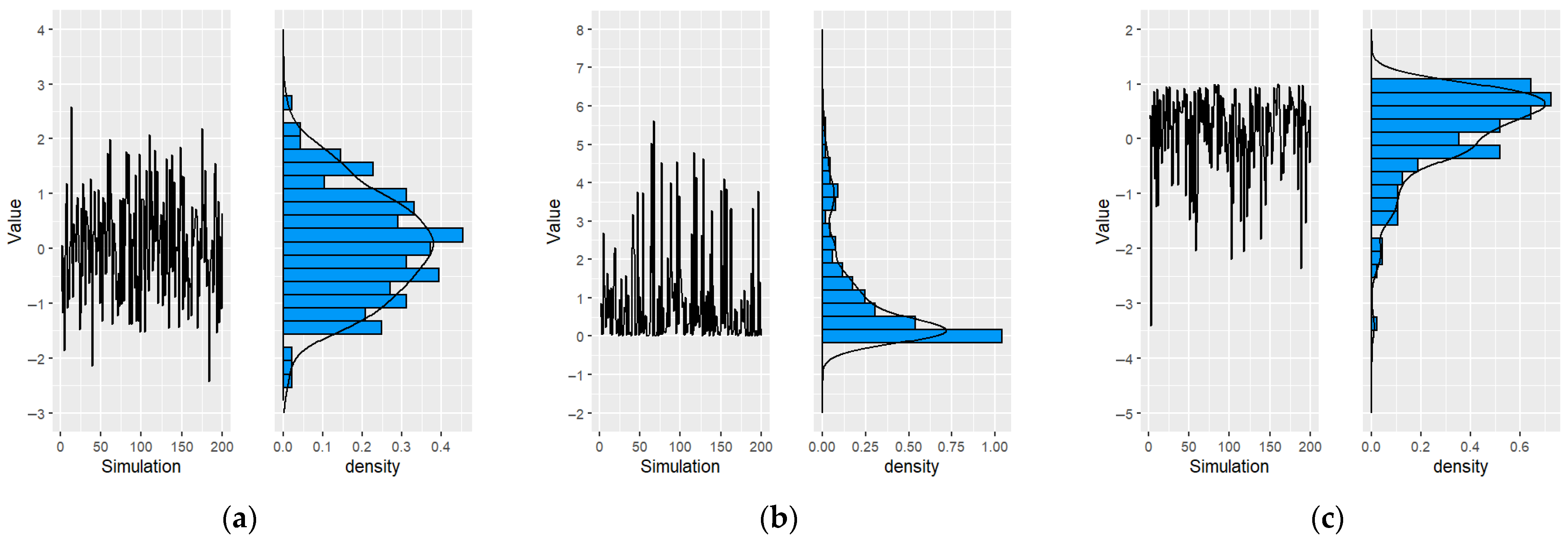
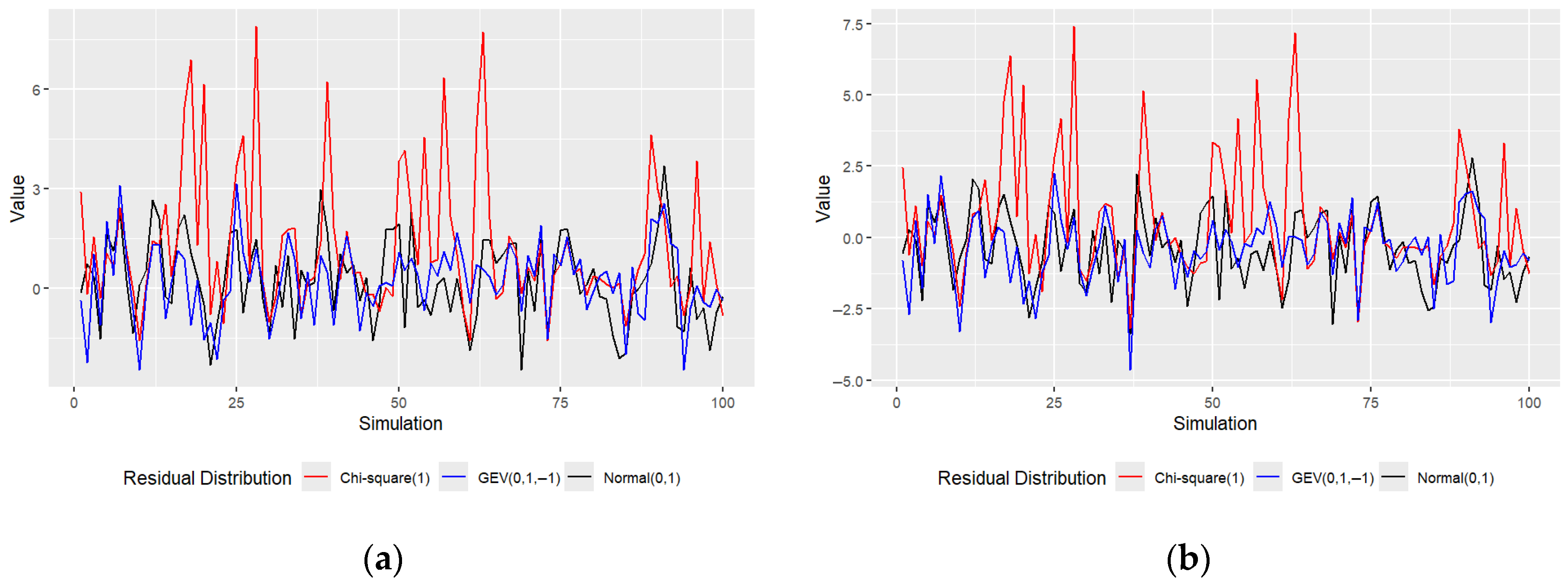
Data generation is intended to generate residuals according to the predetermined true model, with an initial generated data set of 100 observations for both the response and predictor variables. Burn-in is performed on the first 100 observations from the generated data to eliminate the effects of the initial values applied. Next, calculate the true observation (response) values, both linear and nonlinear, according to Equations (16) and (17) and the predetermined residual distribution combinations. Examples of generated residual data and true values are illustrated in Figure 3 and Figure 4, respectively.

In Figure 4a, which represents the true linear model, the generated pattern shows that residuals following the Chi-square(1) distribution (red line) tend to fluctuate with more extreme peaks and move more frequently in the positive direction, consistent with the asymmetric nature of the chi-square distribution, which has only non-negative values. Meanwhile, residuals from the GEV(0,1,−1) distribution (blue line) produce a relatively more symmetric pattern, although they still exhibit some outliers with heavier tails than the normal distribution. Residuals from the Normal(0,1) distribution (black line) display more stable variations, fluctuating around zero with a less extreme spread, thus appearing more consistent with the classical assumptions of the linear model.

In Figure 4b, which depicts the true nonlinear model, the residual pattern also shows differences depending on the distribution used. Residuals with the Chi-square(1) distribution again show a predominance of positive values with significant spikes at certain points, indicating that nonlinearity amplifies the effect of the distribution’s asymmetry. The residuals from the GEV(0,1,−1) distribution appear more volatile than those from the linear model, with some deviations in the more extreme negative direction, consistent with the long-tailed nature of the GEV distribution. Meanwhile, the residuals from the Normal(0,1) distribution still exhibit the most stable pattern, although in the context of the nonlinear model, their variation is slightly greater than that of the linear model, indicating the nonlinear model’s sensitivity to the shape of the residual distribution.

Overall, in both linear and nonlinear models, the residual distribution has a significant influence on the characteristics of the generated results. The normal distribution remains the most stable and conforms to classical assumptions, while the chi-square and GEV distributions exhibit significant deviations, particularly in the form of asymmetry and long tails, with the effects becoming more pronounced in the nonlinear model.

2.

Modeling Setup.

Modeling of the generated data was performed using the ERNN and ERNN-mLASSO models. The applied expectile value of 0.1 was chosen to capture extreme conditions. The activation function used is set to be general (entirely) using tangential hyperbolic (tanh), considering the advantages of tanh which is general—namely, being able to map input values into the range [−1, 1]—thus producing data centered around zero (according to the characteristics of the generated data), accelerating the convergence process, minimizing bias in the gradient, and increasing the stability of network learning compared to the sigmoid activation function which only produces positive output. The number of hidden layers in the ERNN and ERNN-mLASSO models was set (limited) between 4 (the number of inputs) and 8 (twice the number of inputs). The modified LASSO (mLASSO) coefficient value was set to a value limited to the following conditions $\lambda \in \left\{0.1;0.5;1;2;5\right\}$. Next, the characteristics and model parameters, including the number of hidden layer nodes and the mLASSO coefficient value, of each model were optimized using the designed AIC formula.

3.2. Software

All data generation, analysis, model estimation, and visualization were performed using the R programming language (version 4.4.2). The core Expectile Regression Neural Network (ERNN) implementation, with modified LASSO regularization (mLASSO), was custom-built, utilizing several key packages. Specifically, the neural network architecture was built and trained using modified results from the “neuralnet” package. Optimization of a custom Asymmetric Least Squares (ALS) loss function, including the mLASSO penalty term, was performed using optimization routines available in the “stats::nlm” package with some modifications therein.

3.3. Experimental Result

Once the generation data has been obtained and the modeling settings have been defined, the next step is to perform modeling using the predetermined experimental scenarios. The experimental results presented are the accuracy and complexity calculations of the model, as determined by the AIC metric. This section concludes by validating the model’s goodness-of-fit measure using the AIC calculation results, as presented in

Table 2. The results of the calculation of the goodness-of-fit of the model based on the AIC metric.

True Linear Model
Error Distribution	ERNN			ERNN-mLASSO
	J*	AIC		(J*; λ*)	AIC
Normal(0,1)	4	27.11989		(4; 0.5)	13.76294
GEV(0,1,−1)	4	27.84587		(4; 1)	13.36532
Chi-square(1)	4	27.13765		(4; 0.5)	12.59890
True Nonlinear Model
Error distribution	ERNN			ERNN-mLASSO
	J*	AIC		(J*; λ*)	AIC
Normal(0,1)	4	27.55779		(4; 0.5)	14.96016
GEV(0,1,−1)	4	28.07303		(4; 0.5)	13.75278
Chi-square(1)	4	27.54871		(5; 1)	17.48813

Notes: This table compares the performance of the Expectile Regression Neural Network (ERNN) model with its regularized counterpart (ERNN-mLASSO) on simulated data from true linear and nonlinear models with various error distributions. AIC is the Akaike Information Criterion; lower values indicate a better model. J* indicates the optimal number of hidden nodes selected. (J*; λ*) indicates the optimal combination of hidden nodes and mLASSO regularization coefficients. The results show that ERNN-mLASSO consistently produces significantly lower AIC values, indicating superior performance.

.

Table 2 presents the results of the goodness-of-fit model (GOF) calculation based on the AIC to compare the performance of ERNN with its regularized version, ERNN-mLASSO. Experiments were conducted on two types of true models—namely, a linear model and a nonlinear model—with variations in residual distributions including the Normal(0,1), GEV(0,1,−1), and Chi-square(1) distributions. In the true linear model, the AIC values produced by ERNN were in the range of 27.1–27.8 for all error distributions. After applying mLASSO regularization, the AIC values decreased significantly, ranging from 12.59 to 13.76. This decrease indicates that mLASSO is able to improve model efficiency by reducing parameter complexity without sacrificing estimation accuracy. Similar results were also observed in the true nonlinear model, where ERNN produced an AIC of around 27.5–28.1, while ERNN-mLASSO produced a much lower AIC value, ranging from 13.75 to 17.49. This consistent difference confirms that mLASSO regularization is effective in improving ERNN performance, both on linear and nonlinear models. Overall, the consistent pattern of results indicates that integrating mLASSO into ERNN can substantially reduce AIC values across a range of error distributions. This confirms mLASSO’s effectiveness in addressing overfitting while improving model generalization.

4. Empirical Result and Discussion: Stock Market Index

4.1. Data

The empirical application focuses on several stock indices from several countries worldwide; in particular, five stock indices were selected. Details of the empirical data are presented in

Table 3. List of global stock indices used in this research.

Stock Index	Ticker	Country/Region
Indonesian Stock Index (Jakarta Composite)	JKSE	Indonesia
Standard & Poor’s 500	GSPC	United States of America
Deutscher Aktienindex (DAX)	GDAXI	Germany
Financial Times Stock Exchange 100 (FTSE 100)	FTSE	Great Britain
Nikkei 225	N225	Japan

. The selection of these five stock indices was strategically designed to create a representative microcosm of the global financial network, encompassing geographic diversity and levels of economic development. The first four indices—GSPC (United States), GDAXI (Germany), FTSE (United Kingdom), and N225 (Japan)—were chosen as proxies for the world’s most dominant developed markets, representing major financial centers in North America, Europe, and Asia, respectively. Given their substantial market capitalization and high degree of integration into the global financial system, these indices are hypothesized to act primarily as sources or spreaders of systemic risk. To create a crucial point of contrast and analyze the dynamics of risk acceptance, the Indonesian Composite Stock Price Index (JKSE) is included to represent a significant emerging market. As Southeast Asia’s largest economy and a key player in the ASEAN bloc, Indonesia serves as a relevant case study for understanding how global shocks propagate to impact developing countries. The inclusion of markets like Indonesia is vital for a holistic analysis, as it enables the study to empirically investigate the often-asymmetric relationship between developed “core” markets and emerging “periphery” markets. Therefore, conclusions drawn from its role as a risk taker can be generalized to provide important insights into vulnerabilities in the broader emerging market landscape for an international audience. Collectively, this diverse index portfolio provides a robust framework for mapping complex risk transmission pathways and vulnerabilities across various segments of the global stock market.

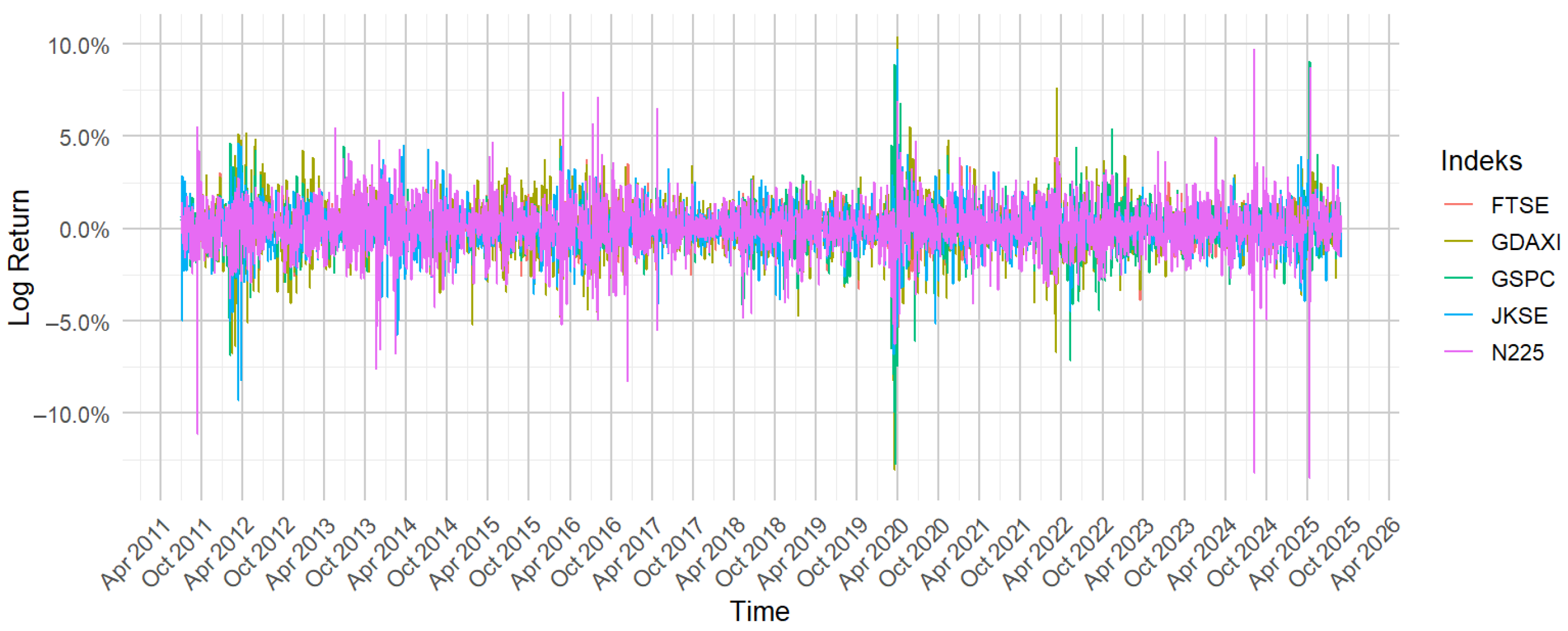
The data used are daily closing prices downloaded directly from the Yahoo Finance database using the “quantmod” package in R software. The observation period selected is from 1 January 2011 to 31 August 2025. This period is chosen with the intention of enabling the data to capture market dynamics under various conditions, including phases of economic expansion and contraction, as well as periods of relevant global financial shocks, such as the COVID-19 pandemic and geopolitical uncertainties that affect global stock market volatility. Each index time series is analyzed in its local currency as reported by the data source. Specifically, GSPC is analyzed in US Dollars (USD), GDAXI in Euros (EUR), FTSE in Pound Sterling (GBP), N225 in Japanese Yen (JPY), and JKSE in Indonesian Rupiah (IDR). No conversion to a common currency is performed in this analysis. The data series used are price return indices, which reflect the change in the capital value of the index components, excluding dividend payments. For each series in its local currency, daily logarithmic returns are calculated using the standard formula $r_t=\ln \left(p_t/p_{t-1}\right)\times 100\%$, where $p_t$ is the closing price on the day $t$ in the local currency. This transformation is used to stabilize variance and produce continuously composite returns. The processed data are the results of daily log return calculations, each of which is illustrated using an overlay time series plot shown in Figure 5.

Figure 5 illustrates the dynamics of daily log returns for five global stock indices, from January 2011 to August 2025. Generally, daily returns for all indices fluctuate around zero, reflecting the short-term nature of stock markets, which are characterized by random fluctuations. However, at certain points in time, there are significant spikes in volatility, consistent with relevant periods of global financial turmoil. During the 2011–2012 period, increased volatility was observed in relation to the European debt crisis, with European markets (GDAXI and FTSE) exhibiting sharper returns than other markets. Between 2014 and 2016, a pattern of increasing fluctuations reappeared, coinciding with the decline in global oil and commodity prices, which affected the Jakarta Composite Index (JKSE) and the Nikkei 225 (N225) due to their high dependence on commodities and international trade.

The most extreme spike in volatility occurred in early 2020, when the COVID-19 pandemic had a profound impact on the world. Nearly all indices experienced sharply negative returns within a short period, indicating global market panic. A gradual recovery was observed in the subsequent period, in line with fiscal/monetary stimulus, as well as vaccine developments. Volatility increased again in 2022, in line with Russia’s invasion of Ukraine and the accompanying energy market turmoil. The GDAXI and FTSE indices exhibited a stronger impact due to their close connection with the European economy. Furthermore, the 2022–2024 period was also marked by high volatility due to rising global inflation and the implementation of high-interest rate policies by major central banks. Until early 2025, the return pattern indicates that the market is still experiencing moderate fluctuations, although geopolitical uncertainty and a global economic slowdown remain risk factors. Thus, this graph not only illustrates the short-term dynamics of stock returns but also reflects how global macroeconomic and geopolitical events directly impact financial market volatility in various regions. This underscores the importance of systemic risk analysis, which links the interdependence of global stock markets, as shocks in one region can quickly spread and affect other markets.

4.2. Modeling Scenario and Result

This section explains the ERNN- and ERNN-mLASSO modeling scenarios, specifically for TERES estimation. TERES estimation based on ERNN or ERNN-mLASSO involves several hyperparameter tunings. The most crucial part of NN modeling is selecting the architecture that produces the best predictions and forecasts. This study employs the moving window concept to evaluate the ERNN and ERNN-mLASSO models based on the hyperparameters that have been set. The hyperparameters for both the ERNN and ERNN-mLASSO models are set as shown in

Table 4. The hyperparameter setting values of the ERNN and ERNN-mL models.

Symbol	Value	Description
J	{4, 5, 6, 7, 8}	Number of nodes in the hidden layer. Set to equal the number of inputs (4) or twice as many (8).
seed	{1, 2, …, 100}	Initial value lock for modeling. Set to 100 unique initial values.
λ	{0, 0.01, 0.5, 1, 5, 10}	Lagrange coefficient for modified LASSO regularization (mLASSO). If λ = 0, it indicates a model without regularization (or ERNN), and if λ > 0, it indicates a model with regularization (or ERNN-mLASSO).
τ	{0.1}	Expectile value. Set to capture extreme expectiles at the 5% level.

.

Overall, Table 4 shows that the study integrates neural network architecture design through setting the number of hidden nodes (J) and seed variations to ensure consistency of results, the mLASSO regularization technique (λ) to control complexity while preventing overfitting, and the expectile-based extreme distribution approach (τ) to emphasize the analysis on the risk of losses located in the tail of the distribution. The combination of these three aspects makes the built model not only flexible in capturing nonlinear patterns in financial market data, but also robust in dealing with volatility and systemic risks originating from extreme events.

Next, the data is divided into two parts: training and testing. The training data is used to estimate the model, while the testing data is used to evaluate the model. This study also uses the concept of a moving window to obtain comprehensive evaluation values. This means that cross-validation is also used in model evaluation. An illustration of the moving window is presented in Figure 6.

Figure 6 shows a visualization of the model selection scheme using the moving window technique, a validation strategy for time series data. Each row in the figure represents one modeling cycle, where the model is trained using a set of historical data (blue blocks) and then tested on the next period (red blocks). As time progresses, the training and testing windows shift forward by the same size. This means that old data is discarded, and new data is added over time. This scheme mimics real-world forecasting conditions, where the model is trained on the most recent available data and used to predict future values. This technique is very useful for evaluating model performance in out-of-sample conditions and capturing the dynamics of changes in data behavior over time.

The measure used to evaluate model forecasts is the average expected loss (AEL) calculated on the testing data. The AEL is calculated using the following formula:

$$AE{L}_p={\displaystyle \frac{1}{N_{testing}}}{\displaystyle \sum _{t\in N_{testing}}{\rho }_{\tau }^E\left(y_{p,t}-\widehat{E}\left(y_{p,t};\tau \right)\right)},$$

(19)

where $N_{testing}$ denotes the number of observations in the testing data. After calculating the AEL, the Diebold and Mariano (DM) test was applied to compare forecast performance. The test statistics are based on the difference in AEL results for each window between the ERNN-mLASSO and ERNN models, as well as between the ERNN-mLASSO and QVAR models, with a significance level of 5%. The test results are presented in

Table 5. Diebold-Mariano test results for AEL.

Index	ERNN-mLASSO vs. ERNN		ERNN-mLASSO vs. QVAR
	Statistics	p-Value	Statistics	p-Value
JKSE	−1.20	0.230	−49.33	0.000
GSPC	−1.08	0.280	−47.84	0.000
GDAXI	−1.31	0.190	−72.97	0.000
FTSE	−1.23	0.220	−73.19	0.000
N225	−1.11	0.267	−55.42	0.000

.

Table 5 presents the results of the DM statistical test used to compare the forecast accuracy of the ERNN-mLASSO model with that of two other models: ERNN (without regularization) and the quantile-based model, i.e., QVAR, on five stock indices. The negative DM statistical values for all indices indicate that the ERNN-mLASSO model tends to produce smaller forecast errors than all other models. The difference between ERNN-mLASSO and the traditional linear model (QVAR) is very large, as indicated by the test significance value of zero. However, when compared with the ERNN model, the differences obtained are not statistically significant, as indicated by the p-values, which are all greater than 5%. To ensure the goodness-of-fit of the ERNN-mLASSO model, the DM test was applied to compare the goodness-of-fit of the models by calculating the AIC value. The test statistics are based on the difference in AIC results between the ERNN and ERNN-mLASSO models in each window, with a significance level of 5%. The test results are given in

Table 6. Diebold–Mariano test results for AIC of ERNN and ERNN-mLASSO.

Index	ERNN-mLASSO vs. ERNN
	Statistics	p-Value
JKSE	−3.01	0.003
GSPC	−2.88	0.004
GDAXI	−2.71	0.007
FTSE	−2.94	0.003
N225	−3.22	0.001

.

Table 6 shows the results of the Diebold-Mariano test to compare the performance of two predictive models based on AIC values on five stock indices. All DM statistical values are negative, and the p-value is <0.05, indicating that the difference between the ERNN and ERNN-mLASSO models is statistically significant at the 5% significance level. The interpretation of the negative statistical values is that the ERNN-mLASSO model consistently produces a smaller AIC than the standard ERNN. This means that ERNN-mL provides a better fit with a lower model complexity penalty. Therefore, it can be concluded that the ERNN-mL model is not only more accurate than ERNN (but not significantly), but also architecturally efficient. In particular, the N225 index shows the most significant result (statistic = −3.22, p = 0.001), indicating the strongest superiority of ERNN-mLASSO in the Japanese market. Other indices such as the JKSE, GSPC, GDAXI, and FTSE also show statistically significant differences.

4.3. Estimation and Discussion Result

This section specifically analyzes and discusses the research results. It begins with the presentation and selection of more stable Expectile-based Value at Risk (EVaR) and Tail Event Risk Expectile Shortfall (TERES) estimates, using either the ERNN or ERNN-mLASSO models. This is followed by the estimation of systemic risk indices based on the SFI and SHI measures. Finally, the section concludes with a comprehensive interpretation of systemic risk through the estimated SNRI movements.

4.3.1. EVaR and TERES

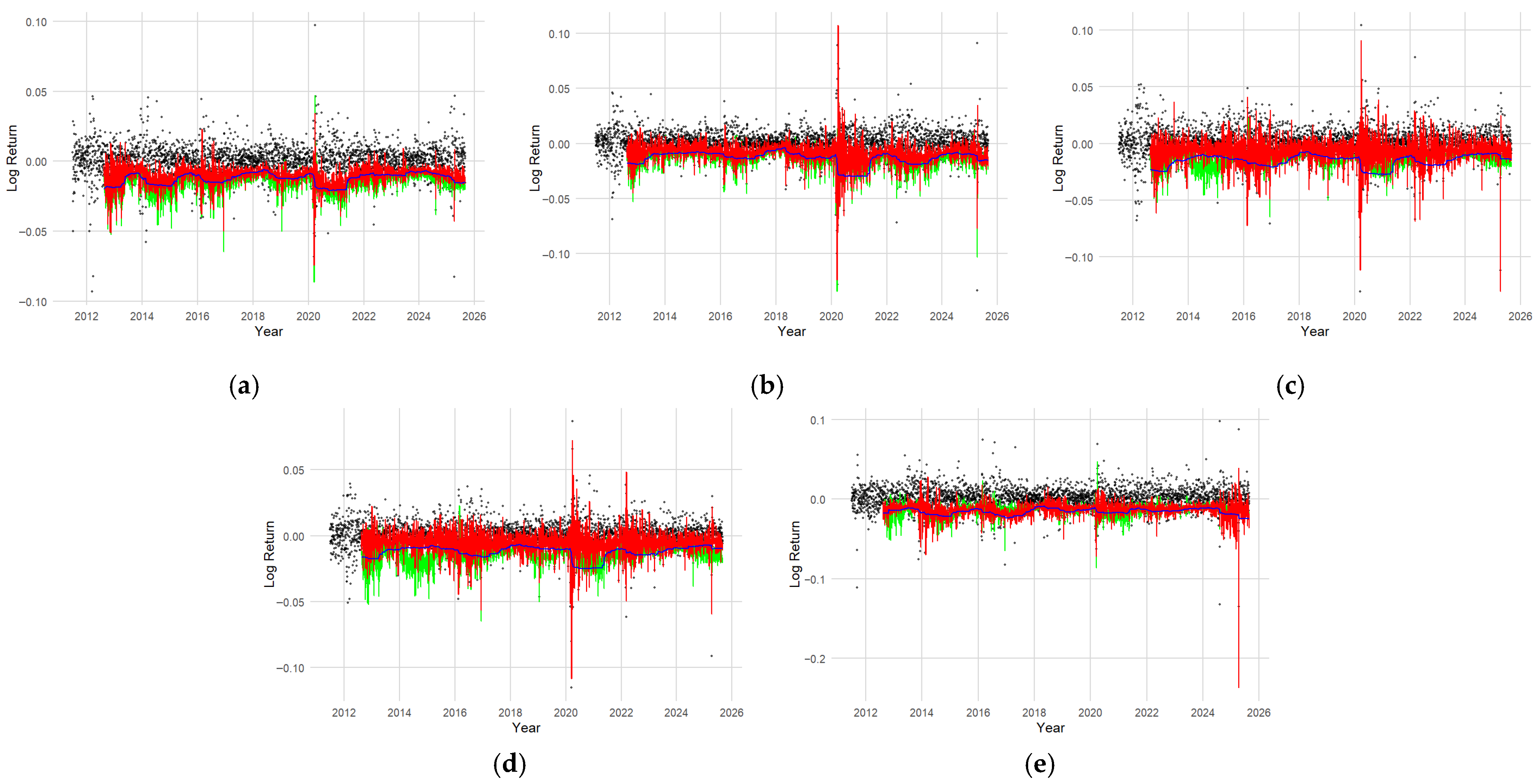
Systemic risk is a measure calculated from the EVaR and TERES functions. A 10% expectile level was chosen as the extreme expectile sample analyzed. The EVaR and TERES estimation results for each stock index are illustrated in Figure 7.

Figure 7 displays the daily log-return, EVaR, and TERES for five global stock market indices. The black dots represent the daily log-return, while the blue line shows the dynamic estimate of EVaR at a 10% expectancy level, which serves as a threshold for extreme losses. The green and red lines show the TERES based on the ERNN and ERNN-mLASSO models, respectively. These two lines measure the expected loss when the EVaR threshold is exceeded.

Overall, all indices fluctuate around zero, but volatility increases sharply during periods of global crises. The EVaR line provides a lower bound marking the threshold for extreme risk, while TERES indicates the severity of losses when this threshold is exceeded. It is important to note the comparison between the green line (TERES from the ERNN model) and the red line (TERES from the ERNN-mLASSO model). The ERNN-mLASSO model, which uses regularization, tends to produce more stable and robust TERES estimates, as evidenced by the smoother and less volatile red line compared to the green line. This suggests that ERNN-mLASSO is more effective at addressing overfitting, where the standard ERNN model (green line) may be too sensitive to noise in the data, resulting in more volatile and less reliable estimates, especially during periods of market volatility. In other words, the ERNN-mLASSO model exhibits better resilience to data anomalies, providing a clearer picture of the true tail risk.

For the JKSE, significant spikes in TERES (both green and red) occurred in early 2020 during the COVID-19 pandemic, and again in 2022 following Russia’s invasion of Ukraine, highlighting the vulnerability of the domestic market to external shocks. A similar pattern is observed in the GSPC, with a sharp decline in March 2020 reflecting US market panic, as well as increased risk during periods of high inflation and monetary policy tightening in 2022–2023. Here, the red line (ERNN-mLASSO) often shows better stability than the green line (ERNN) in estimating these risk peaks. European markets, represented by the GDAXI and FTSE, also exhibit high sensitivity to crises, particularly the 2011–2012 European debt crisis and the Russian invasion of Ukraine in 2022. The red line in the GDAXI indicates a more measured risk severity than the green line, which may be overly reactive. Although the FTSE appears more stable than the GDAXI due to its broader UK market diversification, the volatility difference between the green and red TERES estimates remains noticeable, with the red being more consistent. Meanwhile, the N225 index exhibits a sharp response to the global crisis, with significant spikes in TERES in 2020 and 2022, followed by a sharp decline in 2025. This latest decline is a result of a combination of risk factors, including a slowdown in the Japanese domestic economy, pressure from the strengthening US dollar against the yen, and investor concerns about prolonged global uncertainty, underscoring the Japanese market’s high sensitivity to external shocks. Again, the red line provides a more restrained and likely more accurate estimate of the magnitude of this risk.

Overall, the consistent pattern across these five indices confirms that EVaR serves effectively as a threshold indicator for extreme risk, while TERES provides a more in-depth view of loss severity. A comparison of TERES estimates from the ERNN (green) and ERNN-mLASSO (red) models highlights the advantage of the regularized model in producing more stable and robust risk estimates, reducing the potential for overfitting, and providing a more reliable view of systemic risk in global markets. In complex tail risk measures such as TERES, selecting a robust model is crucial. The ERNN-mLASSO model, with its adaptive regularization and feature selection capabilities, has been shown to provide more stable, less volatile, and more reliable TERES estimates than standard ERNN models. This stability is crucial in risk analysis, where models that are too sensitive to short-term fluctuations or data noise can lead to misleading risk interpretations. Therefore, the TERES generated by the ERNN-mLASSO model (red line) is a superior choice for measuring and understanding the severity of losses in financial markets, due to its ability to distinguish between true risk signals and irrelevant random variability. Therefore, the TERES generated by the ERNN-mLASSO model (red line) will be selected for further risk analysis in a systemic context.

4.3.2. Position and Role of Index in the Context of Systemic Risk

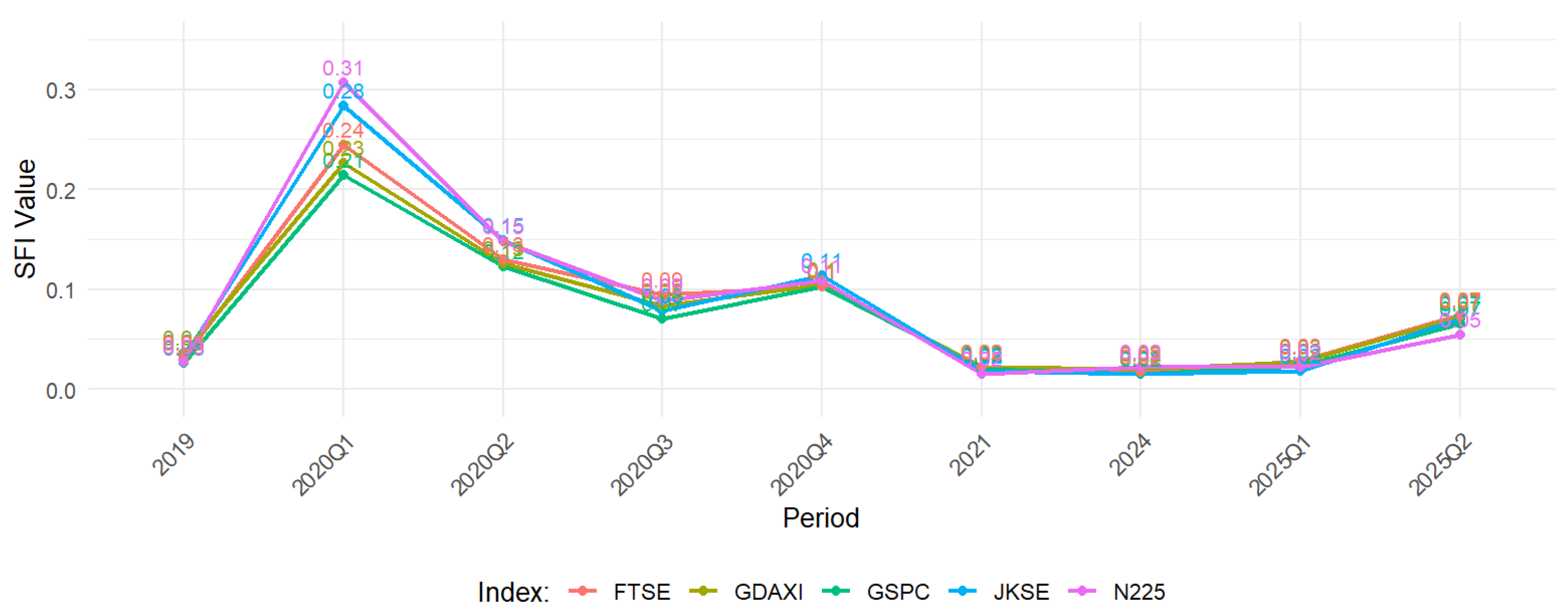
This section is the most important part of this research. It discusses the position and role of each stock index within the context of systemic risk. The analysis begins with estimating the SFI value, which is considered capable of describing the relative position and role of each index within the context of systemic vulnerability. A high SFI value reflects increased exposure to global shocks and the potential for risk transmission between markets. The visualization of the SFI movement is shown in Figure 8, which serves as the basis for identifying the dynamics of systemic fragility before, during, and after the COVID-19 crisis, including the impact of geopolitical uncertainty in 2025.

Figure 8 illustrates the dynamics of five global stock indices based on their respective SFI values from 2019 to 2025Q2. The observation focuses on the phases before, during, and after the global crisis caused by the COVID-19 pandemic. The SFI reflects the level of market vulnerability to systemic turmoil, with higher values indicating greater vulnerability of an index when global financial markets experience collective stress. In other words, a high SFI indicates that an index is more susceptible to contagion effects from other stressed markets, significantly contributes to global financial system instability, and reflects a decline in market resilience in the face of external and internal shocks. Conversely, a low SFI value indicates relatively low systemic vulnerability and greater market stability. The results show that the largest spike occurred in the first quarter of 2020 (2020Q1), coinciding with the peak of the pandemic crisis. During this period, all indices experienced significant increases in SFI values. The N225 and JKSE indices reached their highest levels, indicating greater systemic vulnerability, likely due to their relatively smaller market structures and lower liquidity compared to major global indices. Conversely, indices such as the GSPC and GDAXI tended to have lower SFI values, although they remained elevated during the crisis. This can be attributed to their large market capitalization, market depth, and high liquidity, which enable them to absorb shocks better. After the peak of the crisis, the SFI values across all indices gradually declined, with a sharp decline from 2020Q3 to 2021, in line with the easing of global pressures and the introduction of economic stabilization policies in various countries. Throughout 2021 and 2024, the SFI values remained relatively low and stable, indicating a post-pandemic market resilience phase. However, in early 2025, particularly in the second quarter, a slight increase in SFI values across all indices was observed. Although not as large as the spike during the pandemic, this condition remains significant because it is linked to increasing geopolitical uncertainties affecting the global economy, such as trade tensions, regional geopolitical conflicts, and changes in monetary policy direction in several major countries, all of which increase the potential for cross-market risk transmission. Overall, this pattern confirms that systemic vulnerability is dynamic, strongly influenced by global shocks, and moves in unison across indices due to market interconnectedness. Furthermore, differences in SFI values across indices also reflect the influence of market capitalization and liquidity: large-cap markets, such as the GSPC and GDAXI, tend to be more resilient to shocks, while smaller-cap markets, like the JKSE, are more vulnerable to systemic risk propagation. Thus, the SFI is an important measure in understanding how global shocks and geopolitical uncertainty affect the level of systemic fragility in international stock markets.

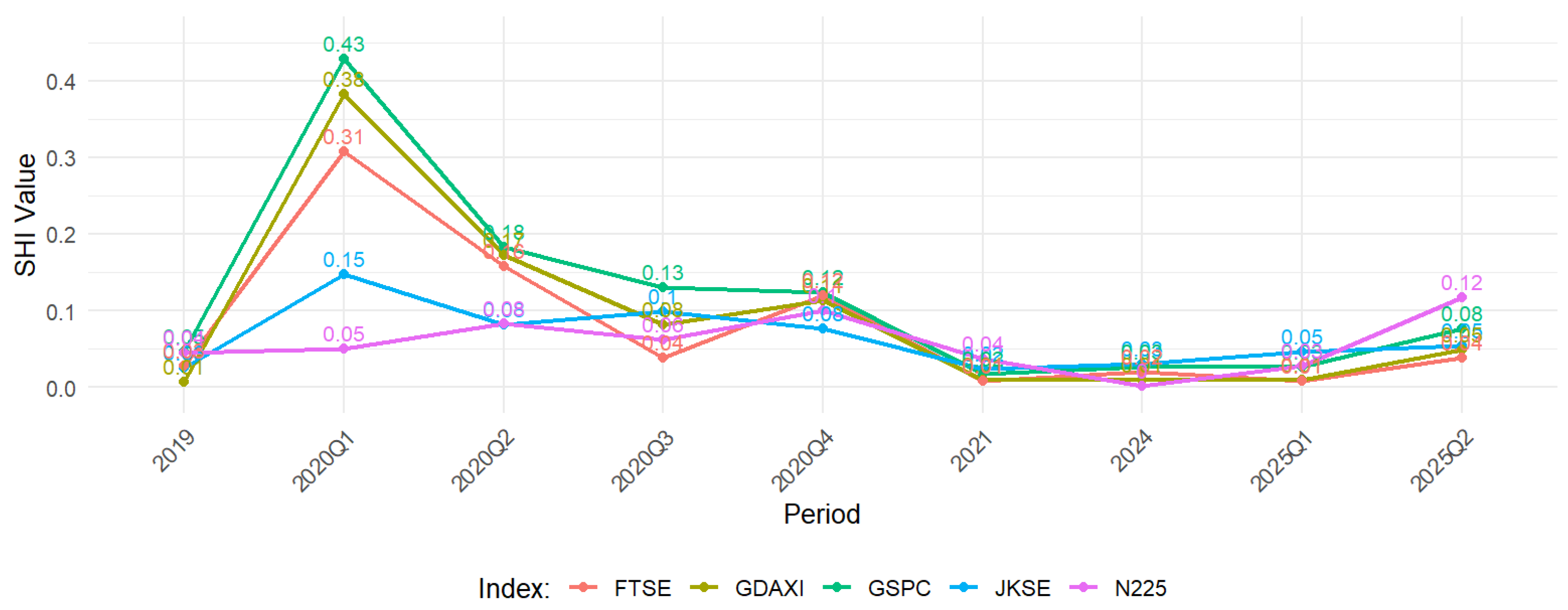
After discussing the SFI, which represents the level of market vulnerability to the propagation of systemic shocks, the next analysis focuses on the SHI. Unlike the SFI, which emphasizes vulnerability, the SHI focuses more on the risk contribution of an index to the overall global financial system. Thus, the SHI provides a complementary perspective on how an index is not only affected by external shocks but also has the potential to become a source of systemic risk transmission to other markets. Visually, the movement of the SHI values for each index is presented in Figure 9.

Figure 9 shows that the peak SHI value occurred in the first quarter of 2020 (2020Q1), which coincided with the initial phase of the COVID-19 pandemic crisis. During this period, the GDAXI (DAX) and FTSE indices recorded the highest SHI values, around 0.43 and 0.31, respectively, indicating that these two indices were major contributors to the spread of systemic risk in global markets. This aligns with their position as representatives of the European market, which has large capitalization and close links to international financial markets. Conversely, indices such as the N225 exhibited relatively low SHI values during the crisis period, indicating a more limited role in spreading systemic turmoil, despite remaining impacted by the global crisis. After the peak crisis phase, SHI values generally trended downward until the period 2021–2024, during which all indices remained at relatively low levels. This reflects the market’s declining ability to transmit systemic risk, alongside the recovery of global economic activity and the implementation of various financial stabilization policies. However, in early 2025, particularly in the second quarter, a slight increase in SHI values was observed in several indices, including the N225, which saw a spike of up to 0.12. While this increase was not as sharp as during the pandemic, the phenomenon remains significant as it is associated with increasing geopolitical uncertainties, such as regional geopolitical tensions, global monetary policy dynamics, and the potential fragmentation of international trade, which again increases the potential for cross-market risk transmission. Thus, this pattern confirms the dynamic nature of the SHI, with large-cap indices, such as the DAX and FTSE, tending to play a dominant role as sources of systemic risk during crises, while smaller-cap indices, like the JKSE, have a more limited contribution. Thus, the SHI complements the SFI analysis by highlighting another dimension of systemic risk: the active role of an index in spreading turmoil to global financial markets.

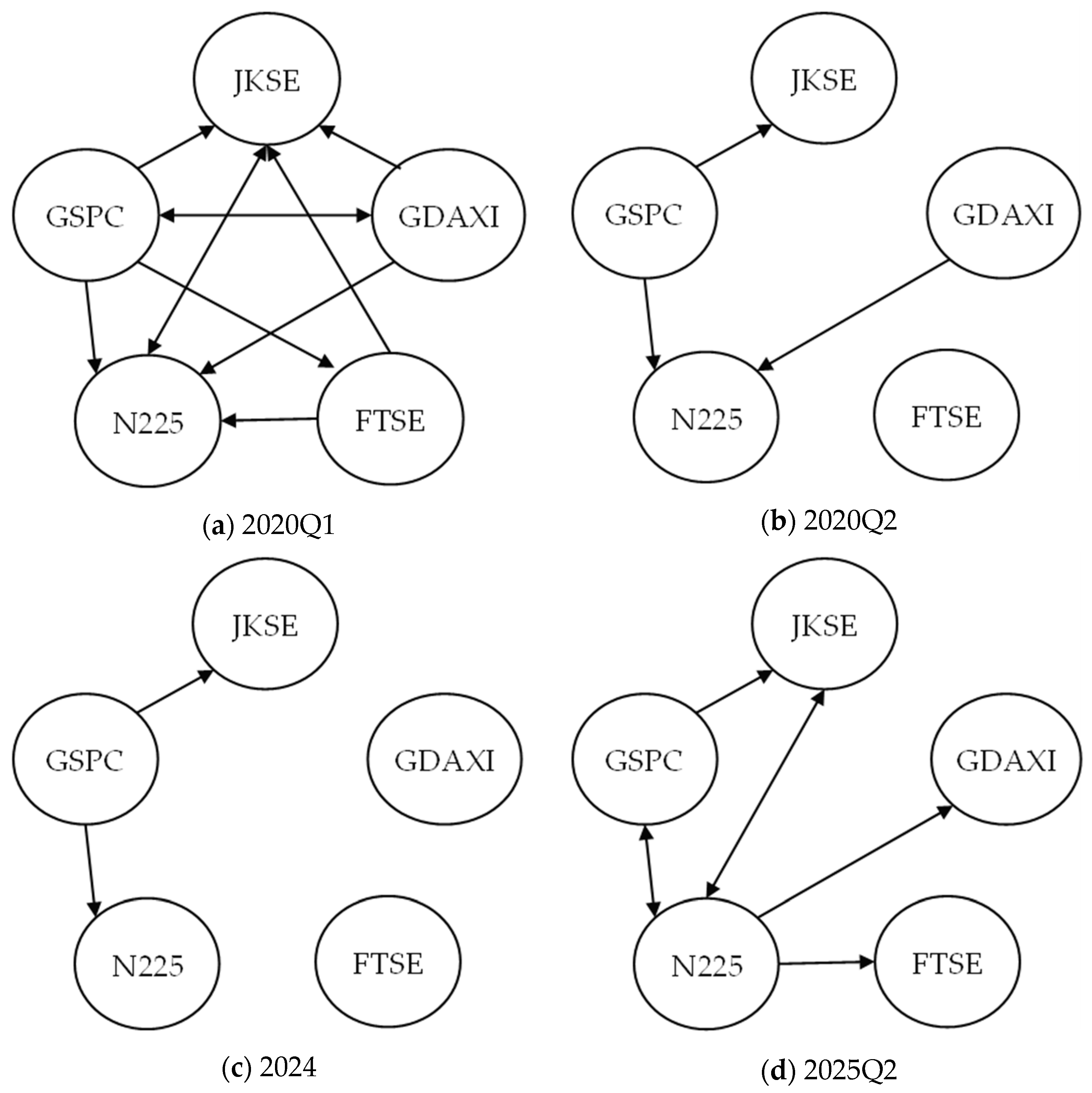
Beyond analyzing the SFI, which provides an aggregate picture of market vulnerability to systemic risk, and the SHI, which measures the contribution of individual indices to the spread of systemic risk, it is important to understand the specific mechanisms by which these risks are transmitted between markets. While the SFI and SHI offer perspectives on the magnitude and source of risk, the dynamics of interconnectivity between markets reveal the pathways and direction of spillovers. Therefore, to gain a comprehensive understanding of systemic risk, analyzing these spillover relationships is crucial. Illustrations of interconnectivity between markets are presented in Figure 10 across several key periods, including the COVID-19 pandemic.

Figure 10 visually depicts the dynamics of risk spillovers across major stock markets—the JKSE, GSPC, GDAXI, FTSE, and N225—showing significant evolution reflecting responses to global economic events. In Q1 2020, which coincided with the escalation of the COVID-19 pandemic, a highly dense and interconnected spillover network was observed. Nearly all markets exhibited bidirectional or unidirectional relationships, indicating rapid and widespread risk transmission amidst global systemic uncertainty. GSPC, in particular, acted as a key trigger, spreading risk to the JKSE, N225, and GDAXI, while N225 also played a central role due to its extensive connectivity. This network density strongly underscores the characteristics of a global crisis, where shocks in one market immediately ripple across others, highlighting the interconnectedness of the global economy.

Moving into Q2 2020, there was a significant de-escalation in the intensity of risk spillovers. The network became sparser, indicating that markets were beginning to adapt or that the initial shock had subsided. The GSPC remains a key hub for risk transmission to the JKSE and N225, but markets like the FTSE appear isolated, indicating potential decoupling or resistance to risk transmission from other hubs. In 2024, the spillover network reached a point of extreme minimalism, maintaining only two unidirectional connections: the GSPC to N225, and the N225 to the JKSE. The GDAXI and FTSE markets were completely disconnected from the network, which could be interpreted as a period of relative stability or increased resilience in these markets. This pattern highlights specific regional risk transmission pathways, with the dominant influence from the US market (GSPC) then channeled through the Asian market (N225) to the Southeast Asian market (JKSE). However, in Q2 2025, spillover connectivity re-emerged, although it has not yet reached the density seen at the start of the pandemic. The GSPC again exerted influence on the N225, and the bidirectional relationship between the JKSE and N225 indicates increasing interdependence. N225 also became a hub for widespread risk transmission, channeling its impact to GDAXI and FTSE, previously isolated markets. This increased connectivity suggests the possibility of a resurgence of global uncertainty or broader market stress, reactivating previously dormant risk transmission channels. The analysis clearly demonstrates the dynamic nature of risk spillovers between stock markets. Crisis periods are characterized by high interconnectivity, while stable periods exhibit network fragmentation. This shift highlights the importance of continuously monitoring the structure of spillover networks to understand and mitigate systemic risk in the evolving global financial markets.

To provide a more comprehensive understanding of the position and role of each global stock index in the context of systemic risk, the SFI and SHI estimation results are integrated. The SFI reflects an index’s vulnerability to systemic shocks, while the SHI indicates an index’s capacity to transmit risk to global markets.

Table 7. Results of the position and role of each index in the context of systemic risk.

Index	SFI	SHI	Systemic Role
JKSE	High	Low	More vulnerable to shocks (risk taker), but its contribution in spreading risk to the global market is relatively limited because its market capitalization is smaller.
GSPC	Low	High	Playing a greater role as a risk transmitter, especially during the 2020 crisis, reflects its strong connection to global markets.
GDAXI	Low	High	Similarly to the GSPC, it plays a significant role in risk transmission, particularly during the pandemic.
FTSE	Moderate	Moderate	Stable, relatively resistant to shocks due to its large market capitalization; however, it can still channel risk moderately.
N225	High	Low	Vulnerable to shocks and starting to play a larger role in risk transmission in 2025, in line with increasing geopolitical uncertainty in Asia.

Notes: This table categorizes each stock index based on its estimated Systemic Fragility Index (SFI) and Systemic Hazard Index (SHI) averages over the crisis period. The SFI measures an index’s vulnerability to external shocks (the risk taker). The SHI measures an index’s risk contribution to the system (the risk spreader). The “High,” “Medium,” and “Low” categories are based on the index’s relative ranking over the observation period.

presents objective results based on several crisis periods that draw particular attention to the position and role of each index in the context of systemic risk. Table 7 summarizes the position and role of each global stock index based on its Systemic Fragility Index (SFI) and Systemic Hazard Index (SHI) values. The results indicate heterogeneity in systemic function across indices, which can be categorized as risk takers and risk transmitters.

The JKSE Index is positioned as a more vulnerable index to shocks (high SFI), but its contribution to spreading systemic risk is relatively limited (low SHI). This is understandable given the JKSE’s smaller market size and capitalization compared to major global indices. Thus, the JKSE is more representative of a market that is sensitive to external pressures but does not act as a center for global risk transmission. Conversely, the GSPC and GDAXI demonstrate a dominant role as risk transmitters. A low SFI indicates relative resilience to shocks, but a high SHI reflects their capacity to channel risk to global markets, particularly during the 2020 crisis. This can be explained by their large market capitalization and the degree of integration of both in the international financial network. Shocks to the GSPC and GDAXI have the potential to cause significant spillover effects on other indices. The FTSE exhibits a moderate profile, both in terms of its SFI and SHI. Its large market capitalization makes it relatively stable against shocks, while still maintaining the ability to transmit moderate levels of risk. This position positions the FTSE as an index with a balancing role in the global financial system, neither dominantly acting as a risk taker nor as a risk transmitter. Meanwhile, the N225 (Nikkei 225) exhibits dual characteristics: it is vulnerable to shocks (high SFI), but its contribution to global risk transmission is initially limited (low SHI). However, since 2025, the N225’s role has increased, as evidenced by the rise in SHI. This increase aligns with increasing geopolitical uncertainty in the Asian region, which has pushed the Japanese market to become more influential in transmitting systemic risk. Overall, this mapping confirms that indices with large market capitalization and high global integration (such as the GSPC and GDAXI) tend to act as risk transmission hubs, while indices with relatively small market capitalizations (such as the JKSE) function more as risk recipients. However, the dynamics of economic and geopolitical conditions, as reflected in the N225, can change the role of an index over time, making continuous monitoring important in systemic risk analysis.

The finding that developed markets like the GSPC and GDAXI serve as primary risk disseminators, while emerging markets like the Jakarta Composite Index (JKSE) act as receivers, provides strong empirical confirmation of the core-periphery model of the global financial network structure. This implies that the stability of peripheral markets, such as Indonesia, is fundamentally dependent on conditions in core financial centers. The implication is that shocks that appear to originate in the US or Europe are not isolated events; they systematically propagate and are amplified in smaller, less liquid markets. This highlights the asymmetry of vulnerability in the global financial system, where geographic diversification may offer less protection for investors in emerging markets than previously thought. Another interesting finding is the projected shift in the role of Nikkei 225 (N225), which begins to exhibit characteristics of a more significant risk disseminator toward 2025. This likely reflects changing macroeconomic dynamics in the Asian region, including increasing geopolitical uncertainty and shifting capital flows. This suggests that a country’s role in the global risk network is not static; These roles can evolve with changing economic and political conditions. This challenges the simplistic view that only the US and European markets are sources of risk, highlighting the importance of dynamically monitoring all major players in the system. The results of this mapping of the roles of spreaders and takers align with the spillover index framework pioneered by Diebold and Yilmaz (2012), which also found that shocks tend to originate in the US market. However, our contribution extends their work by using a nonlinear, machine learning-based approach. Our ERNN-mLASSO model specifically quantifies risk transmission during tail events, which are the most crucial moments for systemic stability. This shows that the ‘core-periphery’ relationship becomes much more pronounced and dangerous precisely during times of extreme market stress, a nuance that linear models may miss.

4.3.3. Systemic Network Risk Estimation

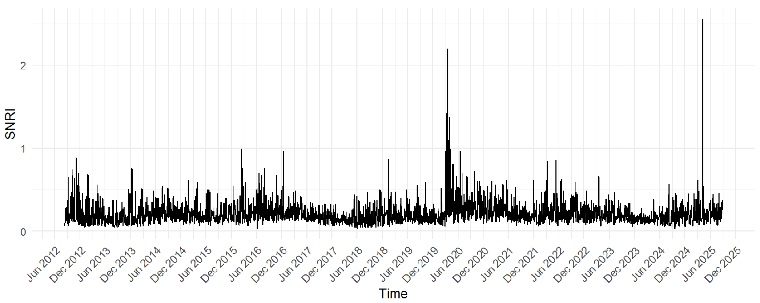
Finally, this study concludes by presenting the movement of the SNRI, which combines both indices (SFI and SHI) within a single network framework. The SNRI not only examines the level of vulnerability or potential danger of each index separately, but also how the index’s relative position within the overall global financial system affects network stability. In other words, the SNRI illustrates the systemic significance of an index within the context of the market interconnected network; namely, how important the index’s role is in maintaining or disrupting the stability of the entire system. Visually, the movement of the obtained SNRI is depicted as in Figure 11.

Figure 11 presents the dynamics of the SNRI from approximately the second quarter of 2012 to the second quarter of 2025. As an aggregate measure integrating vulnerability (SFI) and risk contribution (SHI), the SNRI reflects the systemic significance of the global financial market network as a whole. High SNRI values indicate a highly stressed system, where interconnections between markets amplify rather than mitigate shocks.

The visualization reveals two highly significant spikes during the observation period. The first occurred in the first quarter of 2020, clearly representing a manifestation of the COVID-19 pandemic crisis. The increase in SNRI to above two during this period indicates that these exogenous shocks not only increased the individual vulnerability of each market but also drastically increased the potential for risk contagion within the global network. After this peak, the SNRI value declined and remained stable throughout 2021 and 2023, indicating a phase of system resilience and adaptation to the crisis. The second spike, even more extreme in magnitude, occurred in early 2025. This sharp spike indicated the potential for a systemic shock with impacts exceeding those of the previous pandemic crisis. This drastic increase could be attributed to escalating geopolitical uncertainties, such as widespread regional conflict, the threat of inflation due to high interest rates, or even a monetary policy crisis triggered by tensions between countries in several regions. The high SNRI value at this point indicates that the global financial market network is in a highly fragile state and is at high risk of systemic failure. Overall, this SNRI movement pattern confirms that the stability of the global financial network is dynamic and highly sensitive to macroeconomic and geopolitical shocks. The SNRI serves as an effective early warning indicator in detecting the accumulation of systemic risk at the network level, providing crucial signals for regulators and policymakers.

5. Conclusions

This research makes a significant contribution to systemic risk modeling, particularly in relation to stock indices, by developing a model that can capture information from heavy-tailed distributions while simultaneously considering nonlinear relationships and complexity. By integrating Expectile Regression, which is sensitive to extreme events, with the flexibility of Artificial Neural Networks (ANNs) in capturing nonlinear relationships and the efficiency of Modified LASSO (mLASSO) regularization to prevent overfitting, the proposed model, the ERNN-mLASSO, is proven to overcome the limitations of traditional approaches. Simulation studies consistently show that the ERNN-mLASSO model produces significantly lower AIC values across a wide range of conditions, demonstrating its superiority in accuracy and efficiency compared to the standard ERNN model. This methodological advancement provides a more robust foundation for measuring complex risk dynamics in modern stock markets.

The application of this framework to five major global stock indices (JKSE, GSPC, GDAXI, FTSE, and N225) has yielded in-depth empirical insights into the global risk architecture. Analysis using the Systemic Fragility Index (SFI) and the Systemic Hazard Index (SHI) successfully maps the distinct and dynamic roles of each market. Large-cap developed markets, such as the GSPC and GDAXI, have consistently been identified as dominant risk spreaders, with shocks originating in these markets having a high capacity to spread throughout the system, particularly during periods of crisis such as the COVID-19 pandemic. Conversely, emerging markets, such as the Jakarta Composite Index (JKSE), play a more system-wide role as risk takers, demonstrating greater vulnerability to external shocks despite their more limited contribution to global risk spread. Interestingly, the analysis also captures a shift in the role of the Nikkei, which began to demonstrate increased risk-spread capacity in 2025, coinciding with the growing geopolitical uncertainty in the Asian region. Perhaps the most significant and concerning finding is the dynamics of the Systemic Network Risk Index (SNRI), which serves as a barometer of the aggregate health of the global financial system. The SNRI visualization clearly shows two extreme spikes. The first spike occurred in the first quarter of 2020, accurately reflecting the market panic caused by the COVID-19 pandemic. However, a second spike in early 2025 indicates an even higher level of risk, signaling the potential for a systemic shock whose impact could exceed that of the previous crisis. This drastic increase indicates that the global financial network is in a highly fragile state, likely triggered by the accumulation of geopolitical uncertainty, regional conflicts, and monetary policy tensions between countries. Overall, this research not only offers academic advancement in risk modeling but also provides an efficient diagnostic tool for regulators, policymakers, and investment managers. With its ability to identify key sources of risk, quantify the vulnerability of individual markets, and provide early warning signals of system-wide fragility, the ERNN-mLASSO methodology could be a vital instrument. It could help design more targeted policy interventions to strengthen financial resilience and mitigate the destructive impact of future systemic crises.

While this study provides valuable insights, we acknowledge several limitations that could inform future research. First, our analysis is limited to five stock indices. While representative, this coverage does not encompass other important emerging markets, such as China and India, whose roles in the global risk network are also growing. Second, this study focuses exclusively on stock markets. Systemic risk is a multi-asset phenomenon, and interactions with other asset classes such as bond markets, commodities, and cryptocurrencies are not included in this model. Third, while the ERNN-mLASSO model excels in prediction, its complex machine learning nature limits its causal interpretability. The model can identify risk spreaders, but it does not explicitly explain why or through what specific economic channels the risk propagates. These limitations directly point to several promising research directions. Future research could expand the analysis by incorporating larger and more diverse datasets from global stock markets to validate our findings and map a more comprehensive risk network. Furthermore, a highly relevant research direction is the development of multi-asset models to capture cross-asset risk spillovers, which would provide a more comprehensive picture of financial stability. Finally, integrating explainable Artificial Intelligence (XAI) techniques with the ERNN-mLASSO framework could be an essential next step in enhancing model transparency, strengthening the interpretability of prediction results, and supporting more informed and actionable decision-making regarding risk transmission mechanisms.

References

1. Acharya, V. V., Pedersen, L. H., Philippon, T., & Richardson, M. (2017). Measuring systemic risk. The Review of Financial Studies, 30(1), 2–47. [Google Scholar] [CrossRef]
2. Ahmed, J., & Rura, H. (2024). Understanding heuristics and investor behavior in financial markets. Journal of Policy Options, 7(4), 22–29. [Google Scholar]
3. Allen, F., & Gale, D. (2000). Financial contagion. Journal of Political Economy, 108(1), 1–33. [Google Scholar] [CrossRef]
4. Azmi, U., Siswono, G. O., Syaifudin, W. H., Saputra, W. H., & Ningtyas, P. M. A. (2022). Risk analysis on agricultural commodity portfolio using Value at Risk (VaR) and Expected Shortfall (ES) based on ARIMA-GARCH. AIP Conference Proceedings, 2641(1), 030027. [Google Scholar]
5. Bagirov, M., & Mateus, C. (2025). Modelling volatility spillovers between prices of petroleum and stock sector indices: A multivariate GARCH comparison. Modern Finance, 3(3), 66–111. [Google Scholar] [CrossRef]
6. Billio, M., Getmansky, M., Lo, A. W., & Pelizzon, L. (2012). Econometric measures of connectedness and systemic risk in the finance and insurance sectors. Journal of Financial Economics, 104(3), 535–559. [Google Scholar] [CrossRef]
7. Cannon, A. J. (2011). Quantile regression neural networks: Implementation in R and application to precipitation downscaling. Computers & Geosciences, 37(9), 1277–1284. [Google Scholar] [CrossRef]
8. Chavleishvili, S., & Manganelli, S. (2024). Forecasting and stress testing with quantile vector autoregression. Journal of Applied Econometrics, 39(1), 66–85. [Google Scholar] [CrossRef]
9. Chen, H., & Fan, K. (2022). Tail value-at-risk-based expectiles for extreme risks and their application in distributionally robust portfolio selections. Mathematics, 11(1), 91. [Google Scholar] [CrossRef]
10. Di Bernardino, E., Laloë, T., & Pakzad, C. (2024). Estimation of extreme multivariate expectiles with functional covariates. Journal of Multivariate Analysis, 202, 105292. [Google Scholar] [CrossRef]
11. Diebold, F. X., & Yilmaz, K. (2012). Better to give than to receive: Predictive directional measurement of volatility spillovers. International Journal of Forecasting, 28(1), 57–66. [Google Scholar] [CrossRef]
12. Hong, S. (2022). Essays in applied macroeconomics [Doctoral dissertation, University of Warwick]. [Google Scholar]
13. Iqbal, N., Bouri, E., Grebinevych, O., & Roubaud, D. (2023). Modelling extreme risk spillovers in the commodity markets around crisis periods including COVID19. Annals of Operations Research, 330(1), 305–334. [Google Scholar] [CrossRef]
14. Jiang, C., Jiang, M., Xu, Q., & Huang, X. (2017). Expectile regression neural network model with applications. Neurocomputing, 247, 73–86. [Google Scholar] [CrossRef]
15. Kamah, M., & Riti, J. S. (2024). Measuring the connectedness of the Nigerian banking network and its implications for systemic risk. Modern Finance, 2(2), 96–119. [Google Scholar] [CrossRef]
16. Keilbar, G., & Wang, W. (2022). Modelling systemic risk using neural network quantile regression. Empirical Economics, 62(1), 93–118. [Google Scholar]
17. Lai, Y., & Hu, Y. (2021). A study of systemic risk of global stock markets under COVID-19 based on complex financial networks. Physica A: Statistical Mechanics and Its Applications, 566, 125613. [Google Scholar] [CrossRef]
18. Lee, J. H., Ryu, J., & Tsomocos, D. P. (2013). Measures of systemic risk and financial fragility in Korea. Annals of Finance, 9(4), 757–786. [Google Scholar]
19. Liao, L., Park, C., & Choi, H. (2019). Penalized expectile regression: An alternative to penalized quantile regression. Annals of the Institute of Statistical Mathematics, 71(2), 409–438. [Google Scholar]
20. Lin, J., Tong, X., Li, C., & Lu, Q. (2022). Expectile neural networks for genetic data analysis of complex diseases. IEEE/ACM Transactions on Computational Biology and Bioinformatics, 20(1), 352–359. [Google Scholar] [CrossRef]
21. Marumo, K., & Li, S. (2024). Downside risk in Australian and Japanese stock markets: Evidence based on the expectile regression. Journal of Risk and Financial Management, 17(5), 189. [Google Scholar] [CrossRef]
22. McClellan, M. (2025). AI and financial fragility: A framework for measuring systemic risk in deployment of generative AI for stock price predictions. Journal of Risk and Financial Management, 18(9), 475. [Google Scholar] [CrossRef]
23. Mihoci, A., Härdle, W. K., & Chen, C. Y. H. (2021). TERES: Tail event risk expectile shortfall. Quantitative Finance, 21(3), 449–460. [Google Scholar] [CrossRef]
24. Naeem, M. A., Karim, S., & Tiwari, A. K. (2022). Quantifying systemic risk in US industries using neural network quantile regression. Research in International Business and Finance, 61, 101648. [Google Scholar] [CrossRef]
25. Naeem, M. A., Karim, S., Yarovaya, L., & Lucey, B. M. (2025). Systemic risk contagion of green and Islamic markets with conventional markets. Annals of Operations Research, 347(1), 265–287. [Google Scholar] [CrossRef]
26. Narayan, S., & Kumar, D. (2024). Macroprudential policy and systemic risk in G20 nations. Journal of Financial Stability, 75, 101340. [Google Scholar] [CrossRef]
27. Newey, W. K., & Powell, J. L. (1987). Asymmetric least squares estimation and testing. Econometrica: Journal of the Econometric Society, 55, 819–847. [Google Scholar] [CrossRef]
28. Pagliaro, A. (2025). Artificial intelligence vs. efficient markets: A critical reassessment of predictive models in the big data era. Electronics, 14(9), 1721. [Google Scholar] [CrossRef]
29. Patton, A. J. (2006). Modelling asymmetric exchange rate dependence. International Economic Review, 47(2), 527–556. [Google Scholar] [CrossRef]
30. Saux, P., & Maillard, O. (2023). Risk-aware linear bandits with convex loss. In International conference on artificial intelligence and statistics (pp. 7723–7754). PMLR. [Google Scholar]
31. Syuhada, K., Hakim, A., & Nur’aini, R. (2023). The expected-based value-at-risk and expected shortfall using quantile and expectile with application to electricity market data. Communications in Statistics-Simulation and Computation, 52(7), 3104–3121. [Google Scholar] [CrossRef]
32. Taylor, J. W. (2000). A quantile regression neural network approach to estimating the conditional density of multiperiod returns. Journal of Forecasting, 19(4), 299–311. [Google Scholar] [CrossRef]
33. Ullah, M. (2024). Dynamic connectedness between crypto and conventional financial assets: Novel findings from Russian financial market. Journal of Applied Economic Research, 23(1), 110–135. [Google Scholar] [CrossRef]
34. Waltrup, L. S., Sobotka, F., Kneib, T., & Kauermann, G. (2015). Expectile and quantile regression—David and Goliath? Statistical Modelling, 15(5), 433–456. [Google Scholar] [CrossRef]
35. Yamashita, M. (2025). Risk measure examination for large losses. Mathematics, 13(12), 1974. [Google Scholar] [CrossRef]
36. Zhang, Q., Zhang, Y., Yang, W., & Wang, S. (2024). Tail dependence, risk contagion and industry systemic risk: Based on method of lasso-expectile. International Journal of Financial Engineering, 11(03), 2441003. [Google Scholar] [CrossRef]
Figure 1. Structural flow of the proposed ERNN-mLASSO framework illustrating the generation of expectile-based risk measures (EVaR and TERES) and their integration into systemic risk indicators—Systemic Fragility Index (SFI), Systemic Hazard Index (SHI), and Systemic Network Risk Index (SNRI)—derived from five global stock indices.
Jrfm 18 00593 g001
Figure 2. Illustration of the architecture of the expectile regression neural network model.
Jrfm 18 00593 g002
Figure 3. Visualization of the error generation results, each of which follows the following distribution: (a) Normal(0,1); (b) Chi-square(1); (c) GEV(0,1,−1).
Jrfm 18 00593 g003
Figure 4. Visualization of the results of the true value calculations according to the distribution used for each true model: (a) True linear model; (b) True nonlinear model.
Jrfm 18 00593 g004
Figure 5. Daily log return of five stock indices.
Jrfm 18 00593 g005
Figure 6. Visualization of the model selection scheme using a moving window. Training data (blue) and testing data (red).
Jrfm 18 00593 g006
Figure 7. Illustration of daily log-returns, EVaR, and TERES for the index: (a) JKSE; (b) GSPC; (c) GDAXI; (d) FTSE; (e) N225. Each panel displays a series of daily log returns (black dots). The blue line shows the dynamic estimate of Expectile-based Value at Risk (EVaR) at a 10% expectile level, which serves as a threshold for extreme losses. The green and red lines show the Tail Event Risk Expectile Shortfall (TERES) based on the ERNN and ERNN-mLASSO models, respectively, which both measure the expected loss if the EVaR threshold is exceeded. Peaks in the TERES line (red) indicate periods of severe market stress, where actual losses far exceed the normal risk threshold.
Jrfm 18 00593 g007
Figure 8. Visualization of the movement of the SFI stock index rankings during a certain observation period. The SFI measures a market’s vulnerability to systemic shocks originating in other markets. A higher SFI indicates greater fragility (a risk-taking role). This figure clearly shows the simultaneous spike in SFI for all indices during the first quarter of 2020, which coincided with the peak of the COVID-19 crisis.
Jrfm 18 00593 g008
Figure 9. Visualization of the movement of the SHI stock index rankings during a specific observation period. The SHI measures the risk contribution of a market that has the potential to spread and harm other markets in the network. A higher SHI value indicates that an index acts as a significant source of systemic risk (a role as a risk spreader).
Jrfm 18 00593 g009
Figure 10. Illustration of the dynamics of risk spillover between stock markets in several periods.
Jrfm 18 00593 g010
Figure 11. Visualization of SNRI dynamics throughout the observation period.
Jrfm 18 00593 g011