Article

How Does the Mauritanian Exchange Rate React During a Crisis? The Case of COVID-19

by
Mohamed Said Diah
1,*,†,‡,
Mohamedou Cheikh Tourad
1,‡,
Youssef Lamrani Alaoui
2,‡,
Mohamed Farouk Nanne
1 and
Mohamed Abdallahi Beddi
3
1
Scientific Computing, Computer Science and Data Science Research Unit (CSIDS), Faculty of Science and Technics, Nouakchott University, Nouakchott, Mauritania
2
Ifelab-LERMA, Mohammadia School of Engineering, Mohammed V University, Rabat B.P:8007.N.U, Morocco
3
Geometry, Analysis, Algebra, and Applications (G3A), Faculty of Science and Technics, Nouakchott University, Nouakchott, Mauritania
*
Author to whom correspondence should be addressed.
Current address: Department Matemetical, Faculty of Science and Technics, Nouakchott University, Mauritania.
These authors contributed equally to this work.
J. Risk Financial Manag. 2025, 18(10), 589; https://doi.org/10.3390/jrfm18100589
Submission received: 20 August 2025 / Revised: 5 October 2025 / Accepted: 7 October 2025 / Published: 17 October 2025
(This article belongs to the Section Financial Markets)

Abstract

This paper examines the impact of the COVID-19 pandemic on the volatility of the EUR/MRU and USD/MRU exchange rates using GARCH-type models. Symmetric GARCH(1,1) and asymmetric specifications—EGARCH and GJR-GARCH—are applied to capture potential leverage effects over two periods: pre-COVID (January 2017–December 2019) and COVID (January 2017–December 2021). The results indicate that the pandemic increased short-run volatility for EUR/MRU, while its impact on USD/MRU was comparatively weaker. Asymmetric models reveal that COVID-19 altered the response of volatility to shocks, with EUR/MRU exhibiting heightened sensitivity and USD/MRU showing contrasting asymmetries. In addition, an out-of-sample backtesting exercise confirms the superior predictive performance of asymmetric models, particularly EGARCH for EUR/MRU and GJR-GARCH for USD/MRU. These findings underscore distinct volatility dynamics and the transmission of external shocks in a small open economy during periods of global uncertainty.

1. Introduction

The outbreak of COVID-19 was first detected in December 2019, following reports of an unidentified pneumonia in Wuhan, China. By early January 2020, Chinese officials confirmed that a novel coronavirus—subsequently named SARS-CoV-2—was responsible for the illness. Toward the end of January, the World Health Organization (WHO) declared a public health emergency, and by March, it had formally recognized the outbreak as a global pandemic (WHO, 2020). Over the following months, countries worldwide implemented strict lockdowns and travel restrictions to contain the virus, while healthcare systems faced unprecedented challenges (McKibbin & Fernando, 2020).
The outbreak of COVID-19 caused substantial disruptions in global financial markets and exchange rate dynamics, leading to heightened volatility worldwide (Ghosh, 2020). In the early stages of the crisis, investors flocked to safe-haven assets like the US dollar (USD), Japanese yen (JPY), and Swiss franc (CHF), leading to sharp fluctuations in currency values (Ghosh, 2020). Central banks worldwide, including the Federal Reserve, the European Central Bank (ECB), and the Bank of England (BoE), lowered interest rates to historically low levels to stimulate economic activity, which, in turn, had a depreciating effect on their respective currencies (Cook et al., 2021). According to the October 2021 edition of the World Economic Outlook by the International Monetary Fund (IMF), the global economy contracted by approximately 3.2% in 2020 (CRS, 2021). Between 14 February and 23 March 2020, the Dow Jones Industrial Average (DJIA), along with other major indices, lost approximately one-third of its value (CRS, 2021). However, starting in March, the index began a steady recovery, gaining momentum through the fall. On 9 November 2020, the DJIA surged by nearly 3% following reports that a COVID-19 vaccine had been developed (CRS, 2021).
The currency of Mauritania is the Ouguiya (MRU), and its official exchange rate regime is floating (IMF, 2020). The Central Bank of Mauritania (BCM) intervenes to stabilize the exchange rate and maintain its official reserves, publishing daily on its website the total market bids and asks, the amounts settled at the fixing rate, and a summary of market turnover. Since May 2020, the MRU has appreciated within a 2% band against the US dollar, making the de facto exchange rate regime a “crawl”-type system (IMF, 2020).
In 2021, Mauritania returned to growth (+2.4%), supported by consumption, investment, and the recovery of the services sector, despite a decline in gold production at Taziast (World Bank, 2020). Inflation rose to 3.5%, mainly due to food prices, while the exchange rate remained stable and government measures helped reduce extreme poverty. The pandemic had a significantly lower impact than in 2020 (World Bank, 2020).
In the context of the Mauritanian economy, the COVID-19 pandemic has negatively affected economic activity worldwide, both in terms of global supply and global demand (Ministry of Commerce and Tourism, 2022). Mauritania, like other countries, was also impacted by COVID-19, causing a contraction in economic activity, which spread to all sectors (Ministry of Commerce and Tourism, 2022). At the level of the primary sector, growth stood at −5.4% (Ministry of Commerce and Tourism, 2022).
The fishing sub-sector which experienced a decline in fishing effort which resulted in a drop in exports of around 39.4% (Ministry of Commerce and Tourism, 2022).
At the level of the tertiary sector, which represents more than 42% of overall GDP, the preventive measures taken by the authorities to stem the pandemic have contributed greatly to the underperformance of the sector (Ministry of Commerce and Tourism, 2022).
Services which constitute the most important sub-sector in terms of weight (nearly 20% of GDP). It experienced a decline compared to 2019 to stand at 0.7% (Ministry of Commerce and Tourism, 2022).
Inspired by this context, we investigate the impact of the COVID-19 pandemic on currency markets, with a particular focus on the Mauritanian Ouguiya. This study analyzes the effects of COVID-19 on the exchange rate volatility of the euro and the US dollar against the Ouguiya.
The reported findings are based on a comparison between two distinct periods: one before the onset of COVID-19 and another after its emergence. We analyze these two periods to identify the key changes in volatility parameters. The first period spans from January 2017 to December 2019, a time unaffected by the COVID-19 pandemic, while the second period, covering the COVID-19 era, extends from January 2017 to December 2021. Both symmetric and asymmetric models are employed in this study to conduct the analysis. First, we will outline the theoretical basis of each model. Then, we will assess essential model characteristics, including stationarity, ARCH effects, and autocorrelation. Following this, we will estimate the parameters of the standard GARCH model and subsequently those of the asymmetric models, emphasizing a comparison between the pre-COVID and post-COVID-19 periods. Lastly, we will examine the stylized facts and interpret the findings.
Numerous studies have addressed this topic, producing rich findings that have significantly advanced our understanding of the challenges encountered in empirical analyses of exchange rate dynamics.
The modeling of exchange rate volatility has been a central topic in empirical finance, with ARCH and GARCH-type models providing robust frameworks to capture the persistence and clustering of volatility.
One of the earliest uses of the ARCH model in the context of exchange rates was by Hsieh (1989), in his paper Modeling Heteroscedasticity in Daily Foreign-Exchange Rates. He analyzed daily exchange rate data over a ten-year period for five major currencies to capture time-varying volatility. Dritsaki (2019) investigated monthly returns of the EUR/USD exchange rate from August 1953 to January 2017, using 763 observations. By applying ARCH, GARCH, and EGARCH models, she found that the ARIMA(0,0,1)-EGARCH(1,1) specification provided the best fit for modeling both return behavior and leverage effects. The study also noted that this model’s static forecasting method yielded better results than its dynamic form. In Vietnam, Thuy and Thuy (2019) conducted an empirical analysis on exchange rate volatility using 330 monthly observations from January 1990 to June 2017. Their findings indicated that the ARMA(1,0)-GARCH(1,2) model effectively captured the average behavior and volatility of USD/VND and GBP/VND exchange rates, while the ARMA(1,0)-GARCH(1,1) model was more suitable for JPY/VND and CAD/VND. Epaphra (2017) studied exchange rate fluctuations in Tanzania using daily TZS/USD rates from 4 January 2009, to 27 July 2015. By employing ARCH, GARCH(1,1), and EGARCH models, the study concluded that the GARCH(1,1) model most effectively captured volatility dynamics and exhibited strong forecasting performance. Yunusa (2020) investigated the impact of exchange rate volatility on Nigeria’s crude oil exports to several trading partners—including the UK, USA, Italy, France, Spain, Canada, and Brazil—using monthly data from January 2006 to December 2019. The findings confirmed that exchange rate volatility had a significant impact on oil export volumes across all partners, albeit with varying intensities. Ciftci and Durusu-Ciftci (2021) analyzed the impact of exchange rate volatility on Turkey’s exports to key partners such as Belgium, France, Germany, Italy, Netherlands, Russia, Spain, the UK, and the USA over the 2002–2019 period. The results suggested an inverse effect of volatility depending on the timeframe: while low volatility supported short-term export growth, high volatility was linked to a long-term decline in exports. Benzid (2020) used a GARCH(1,1) model to assess the impact of COVID-19 cases and deaths on exchange rate volatility in the United States. Her findings revealed a positive relationship between rising pandemic indicators and the volatility of the USD/EUR, USD/CNY, and USD/GBP exchange rates. Finally, Enumah and Adewinbi (2022) used symmetric GARCH and asymmetric GJR-GARCH(1,1) and EGARCH(1,1) models to analyze PLN/EUR and PLN/USD exchange rate volatility in Poland between January 2015 and July 2022. The study concluded that USD exchange rates were more sensitive to market events than the EUR, and that volatility effects tended to persist longer after crises, especially for the euro.
These studies on exchange rate volatility provide a foundation for understanding time-varying risk, and similar GARCH-type methodologies have also been applied extensively in the context of stock markets to assess market reactions and volatility patterns. Endri et al. (2021) evaluated the behavior of stock prices on the Indonesia Stock Exchange during the COVID-19 pandemic using an event study approach combined with a GARCH model. By analyzing the Composite Stock Price Index (JCI) and LQ-45 component stocks from 6 January to 16 March 2020, the study showed that returns reacted negatively to the COVID-19 outbreak, and market volatility spiked dramatically. Chen (2023) explored the volatility of S&P 500 returns by applying several GARCH-type models to compare the effects of the 2008 Global Financial Crisis and the COVID-19 crisis. The results highlighted that the GJR-GARCH model performed more effectively during the 2008 period, whereas the EGARCH model performed better amid the COVID-19 crisis. Wang et al. (2021) focused on the Chinese stock market’s volatility by analyzing returns from the Shanghai Composite Index and Shenzhen Component Index. Their findings showed that the ARMA(4,4)-GARCH(1,1) model with a Student’s t-distribution gave the most accurate forecasts for Shanghai, while ARMA(1,1)-TGARCH(1,1) was best suited for Shenzhen’s volatility patterns.
Overall, the literature provides strong evidence that exchange rate and stock market volatilities exhibit persistence, asymmetry, and sensitivity to external shocks. While stock market studies highlight the broader implications of crises on financial stability, the exchange rate literature offers a direct perspective on currency dynamics, making the latter particularly relevant to the Mauritanian context. The present study contributes to this line of research by analyzing the volatility of the Mauritanian Ouguiya exchange rates against the euro and the US dollar before, during, and after the COVID-19 pandemic.

2. Materials and Methods

In 1986, Tim Bollerslev introduced the GARCH model, as an extension of the ARCH model. This model allows the variance dynamics to depend on its own past values and past squared errors. A process ϵ t satisfies the GARCH(p, q) representation if
ϵ t = z t h t
where the conditional variance h t is defined as
h t = α 0 + i = 1 p α i ϵ t i 2 + j = 1 q β j h t j
Here, z t denotes weak white noise such that E ( z t ) = 0 and E ( z t 2 ) = σ 2 . The term h t represents the conditional variance, with the following conditions: α 0 > 0 , α i 0 for i = 1 , 2 , , p , β j 0 for j = 1 , 2 , , q , and i = 1 p α i + j = 1 q β j < 1 .
  • Econometric Interpretation
  • The coefficients α i 0 for i = 1 , 2 , , p must be positive to ensure a positive variance.
  • If an upward or downward shock occurs at time t 1 , it is highly likely that the value of ϵ t will be affected in the same direction, either upwards or downwards.
  • If α i = 0 for i = 1 , 2 , , p , this indicates that the series does not exhibit time-varying variance.
  • This model incorporates lags of the variance as autoregressive terms.
  • The conditional variance h t depends on past shocks, represented by the squared errors ϵ t i 2 , as well as on its own past values at time t j .

2.1. Exponential GARCH Model

Asymmetric GARCH models incorporate asymmetry in the response to price variations. These models are designed to capture the asymmetric responses of changing variance to shocks while ensuring that the variance remains positive. This specification adapts the GARCH model by allowing for negative parameters, thereby lifting the non-negativity constraints typically imposed on the coefficients.
log ( σ t 2 ) = ω + i = 1 p α i | ϵ t i | σ t i E | ϵ t i | σ t i + j = 1 q β j log ( σ t j 2 ) + k = 1 r γ k ϵ t k σ t k
Unlike the classic GARCH model, which directly models σ t 2 , the EGARCH model uses the logarithm of the conditional variance. This ensures positivity of σ t 2 without requiring explicit constraints on the parameters.
Parameters:
  • ω : Constant representing the baseline level of volatility.
  • α i : Coefficients capturing he effect of past past shocks (ARCH terms), measuring the magnitude of past innovations.
  • β j : Coefficients reflecting the persistence or memory effect of volatility through lagged log-variances log ( σ t j 2 ) (GARCH terms).
  • γ k : Asymmetry parameters important for modeling the leverage effect.
  • p: Number of ARCH terms (lags of past shocks).
  • q: Number of GARCH terms (lags of past conditional variances).
  • r: Number of asymmetric terms.
The term γ k ϵ t k σ t k captures the asymmetry in how shocks affect volatility. When γ k < 0 , it means that negative shocks (bad news) cause volatility to rise more than positive shocks of the same magnitude.

2.2. Glosten-Jagannathan-Runkle Model (GJR-GARCH)

The GJR-GARCH model is designed to capture the asymmetric behavior of financial market returns. This model posits that investors respond more strongly to losses than to gains, highlighting the concept of leverage.
A process ϵ t satisfies the GJR-GARCH(p, q) representation if and only if
ϵ t = z t h t
where the conditional variance h t is defined as
h t = α 0 + i = 1 q α i ϵ t i + γ i I ( ϵ t i < 0 ) ϵ t i 2 + j = 1 p β j h t j
In this expression, the normalized residual z t is weak white noise, and I ( ϵ t i < 0 ) denotes the indicator function so that
I ( ϵ t i < 0 ) = 1 if ϵ t i < 0 0 otherwise
The constant γ represents the coefficient of leverage.
In this study, the GARCH models are estimated using the logarithmic returns of the EUR/MRU and USD/MRU exchange rates rather than the raw levels. This approach ensures the stationarity of the series, which is essential for correctly applying conditional volatility models.
We define the logarithmic returns of the exchange rate series as
r t = ln ( P t ) ln ( P t 1 ) ,
where:
  • r t is the logarithmic return at time t,
  • P t is the exchange rate (EUR/MRU or USD/MRU) at time t,
  • P t 1 is the exchange rate at time t 1 .
These returns are used as the dependent variable in all GARCH-type models (GARCH(1,1), EGARCH, GJR-GARCH) to ensure stationarity and proper modeling of conditional volatility. This transformation is standard in financial econometrics and allows the interpretation of shocks in relative terms, facilitating the comparison of volatility dynamics across periods, including pre-COVID and COVID-19.
In this study, the model parameters were estimated using **maximum likelihood estimation (MLE)**, assuming a **conditional normal distribution** for the residuals. Robust standard errors (Bollerslev–Wooldridge) were computed for all model parameters to provide reliable inference in the presence of heteroskedasticity, although only the results with conventional standard errors are presented in the table.

2.3. Data

The analysis in this study is based on daily exchange rates of the euro and the US dollar relative to the Mauritanian Ouguiya (EUR/MRU and USD/MRU), sourced from the Central Bank of Mauritania, which provides open-access data. The dataset was inspected for missing entries and irregularities, and any gaps were filled using linear interpolation to ensure the continuity of the time series.
For volatility analysis, the exchange rate series were converted into logarithms, and returns were calculated using successive log differences.
To assess the effects of the COVID-19 pandemic, the dataset is split into two distinct periods:
  • Pre-COVID period: January 2017–December 2019, representing a period unaffected by the pandemic.
  • COVID period: January 2017–December 2021, encompassing the period before, during, and after the COVID-19 crisis.
This segmentation facilitates a comparative examination of exchange rate behavior across the two periods, with particular attention to the stability of the Mauritanian Ouguiya against both the euro and the US dollar.

Use of R Software

All empirical analyses in this study were performed using the R statistical software (version 4.x). R was chosen for its flexibility, reproducibility, and the availability of advanced econometric and visualization tools. The main package employed for volatility modeling was rugarch, which provides a comprehensive framework for specifying and estimating GARCH-type models through functions such as ugarchspec, ugarchfit, ugarchforecast, and ugarchroll. The forecast package was used for forecasting diagnostics.
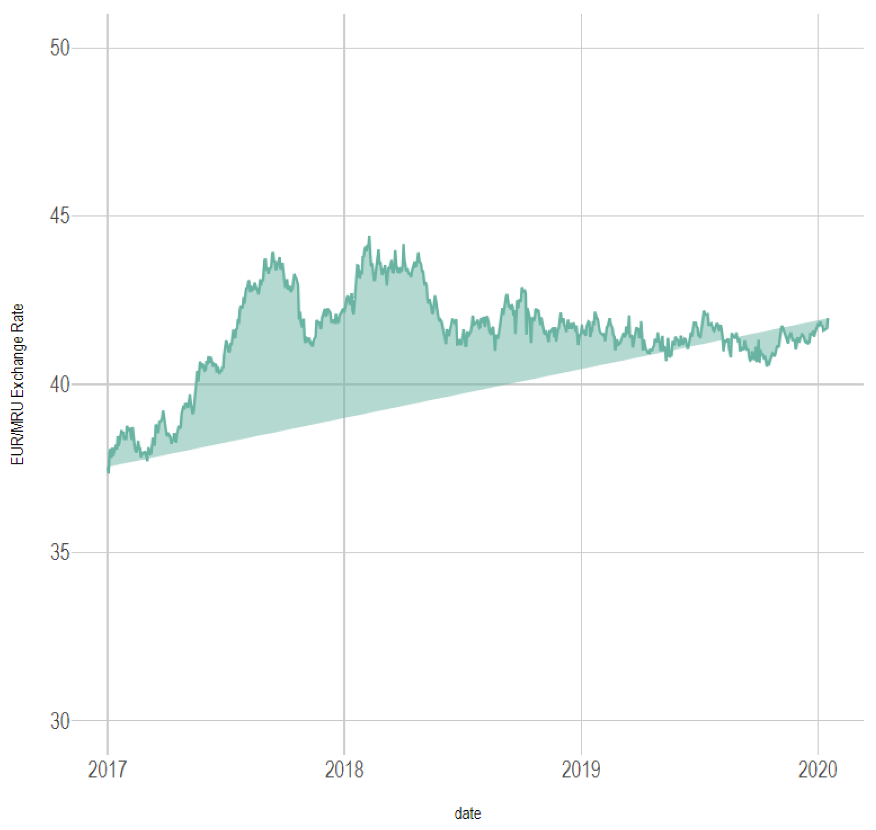
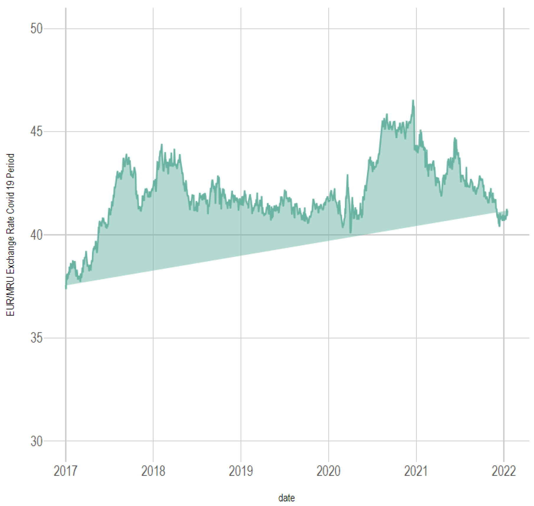
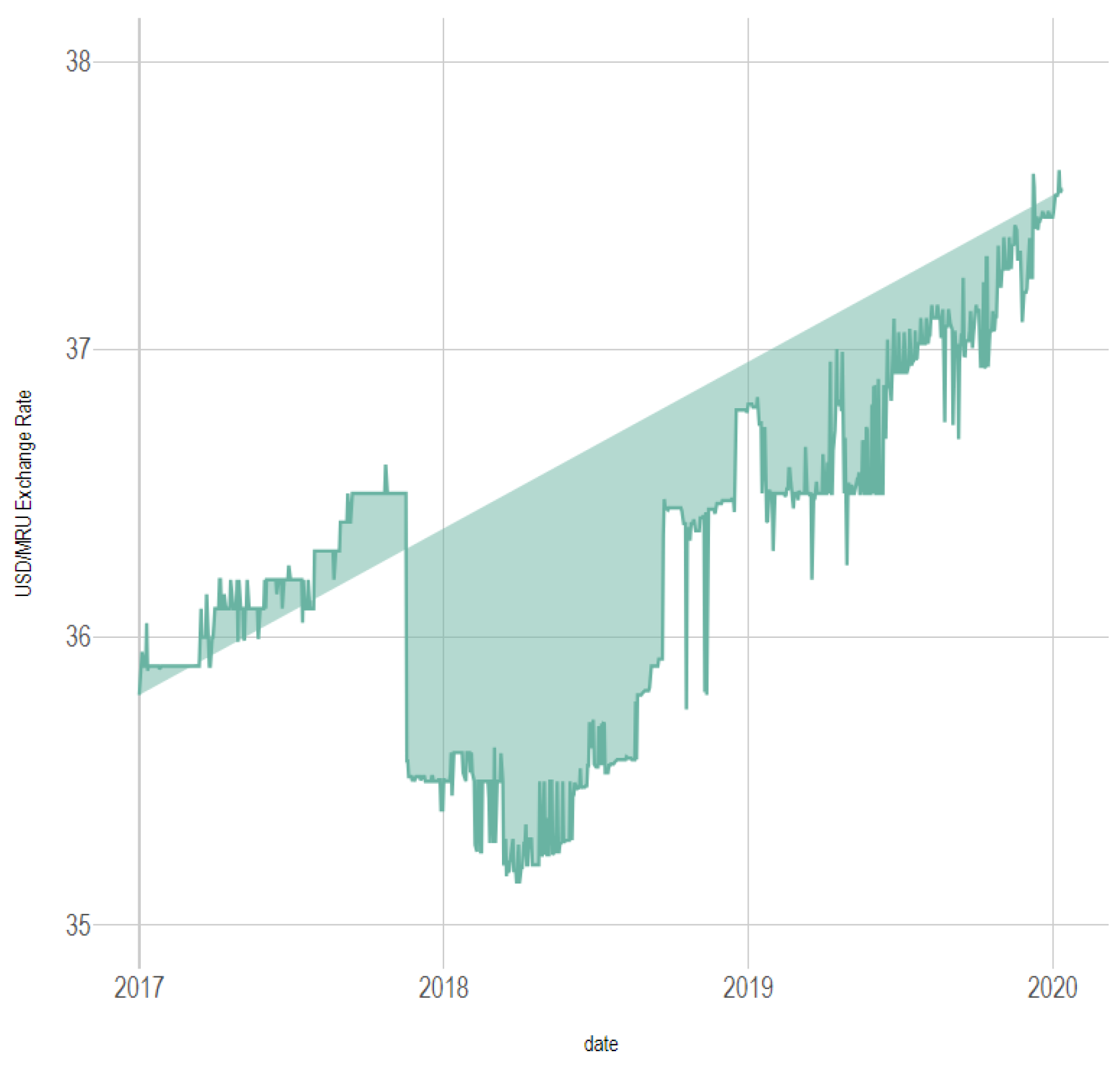
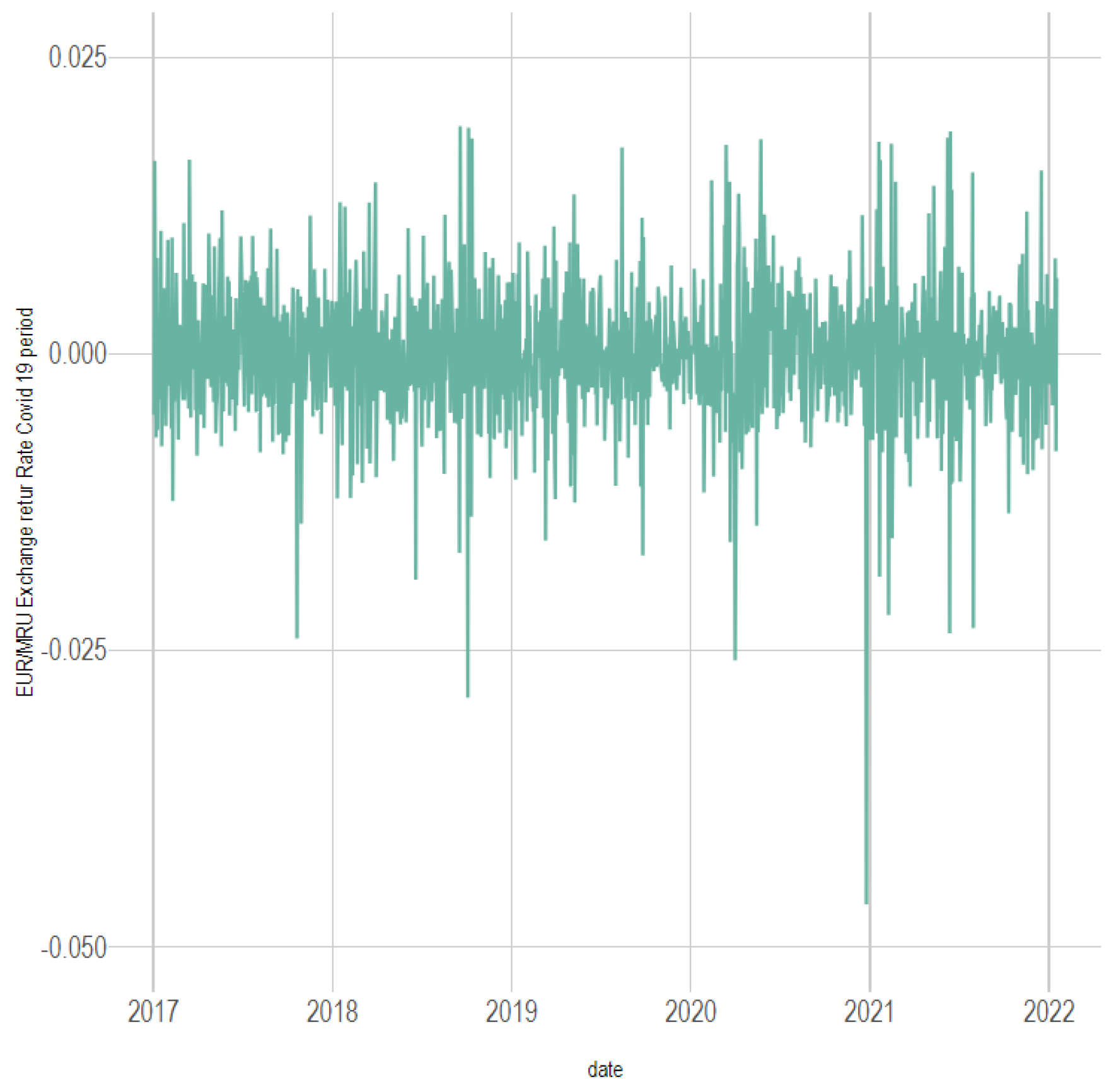
All codes and estimations were executed within R, ensuring full transparency and reproducibility of the empirical results. The exchange rate of the EURO and the USD, respectively, against Ouguiya are presented in the following graphics (Figure 1, Figure 2, Figure 3, Figure 4, Figure 5 and Figure 6):

3. Results

3.1. Descriptive Statistics

In the section bellow, we present some statistics of the EURO/MRU and the USD/MRU Ouguiya daily Return and squared return.
During the pre-COVID period, the EUR/MRU exchange rate exhibited an average daily return of 0.0001429 (see Table 1). a standard deviation of 0.00518, a slight negative skewness of −0.2289, and a kurtosis of 2.61, indicating relatively stable and symmetric behavior. In contrast, during the COVID-19 period (see Table 2), the mean return declined to 0.00007, while volatility increased to 0.00556. The skewness became more negative (−0.6059) and kurtosis rose sharply to 5.87, reflecting stronger downside risk and more frequent extreme fluctuations. These results confirm that the COVID-19 crisis substantially intensified volatility clustering and market instability in the EUR/MRU exchange rate.
During the pre-COVID period (see Table 3), the USD/MRU exchange rate showed an average daily return of 0.0000470, a negative skewness of −0.76, and a high kurtosis of 16.91, indicating frequent extreme negative returns and pronounced leptokurtosis. In contrast, during the COVID-19 period (see Table 4), the mean return declined to 0.000019, while volatility increased (SD = 0.00347). The return distribution became more negatively skewed (−1.73) and highly leptokurtic (kurtosis = 29.43), confirming that the pandemic amplified volatility, downside risks, and extreme price fluctuations in the USD/MRU market.

3.2. Stationarity and ARCH Effect

Both the EUR/MRU exchange rate in the first and second period (COVID-19) pass the ADF test for stationarity, as indicated by their highly negative Dickey–Fuller statistics and p-values of 0.01 (see Table 5 and Table 6).
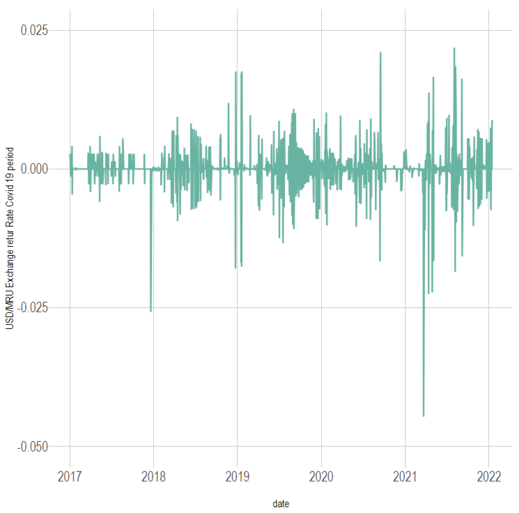
The EUR/MRU exchange rate exhibits the phenomenon of volatility clustering, indicating the potential presence of an ARCH effect in the return series. For a better assessed heteroscedasticity, we examined this return series for ARCH effects.
The result of the ARCH LM test for the euro against the Ouguiya exchange rate during the first period and the COVID-19 period are given as follows:
ARCH LM - test ; Null hypothesis : no ARCH effects
data : EURO / MRU First period
χ 2 = 65.559 , df = 12 , p - value < 2.14 × 10 9
ARCH LM - test ; Null hypothesis : no ARCH effects
data : EURO / MRU COVID - 19 Period
χ 2 = 28.224 , df = 12 , p - value = 0.005129
Given the very small p-value, we reject the null hypothesis and conclude that there is strong evidence of ARCH effects in the EUR/MRU exchange rate during the first period and the COVID-19 period. Given the presence of ARCH effects, it is recommended to model the heteroscedasticity in the data using models like GARCH (Generalized Autoregressive Conditional Heteroskedasticity) to better capture the time-varying volatility.
We observe also that the USD/MRU exchange rate in the first and second period pass the ADF test for stationarity, as indicated by their highly negative Dickey–Fuller statistics with their small p-values. The test of ARCH effect with a small p-value rejects the null hypothesis of no ARCH effect for the two periods.
ARCH LM - test ; Null hypothesis : no ARCH effects
data : USD / MRU First period
χ 2 = 109.8 , df = 12 , p - value < 2.2 × 10 16
ARCH LM - test ; Null hypothesis : no ARCH effects
data : USD / MRU COVID - 19 Period
χ 2 = 37.077 , df = 12 , p - value = 0.0002171

3.3. Autocorrelation

Autocorrelation is the correlation of a time series with its own previous values. When autocorrelation is present in the residuals of a time series, it implies that there is some predictable structure that has not been captured yet by a simple mean (i.e., the data is not white noise). A statistical test such as the Ljung–Box test can be used to test whether autocorrelation exists in the residuals. If this test shows significant autocorrelation at certain lags, it indicates the need for a more complex model (i.e., incorporating ARMA terms) to better capture the data’s underlying structure.
The result of the Box-Ljung test for the Euro/MRU exchange rate in the first and second period are given respectiveley as follows (see Table 7):
Since the p-value is very small (well below 0.05), we reject the null hypothesis. This indicates significant autocorrelation in the residuals up to the 20th lag. This motivates the inclusion of an ARMA model in the mean equation.
The result for the USD/MRU exchange rate in both periods also indicates significant autocorrelation in the residuals up to the 20th lag (see Table 8).

3.4. Estimation of GARCH Models

3.4.1. Standard GARCH Models

Before estimating the GARCH models, we first specified the conditional mean equation by fitting ARMA ( p , q ) models to the EUR/MRU and USD/MRU return series. Model selection was guided by the Akaike Information Criterion (AIC). The results are reported in Table 9.
Exchange Rate Return for EUR/MRU
For EUR/MRU Returns, several ARMA ( p , q ) specifications were tested. Although ARMA(2,1) and ARMA(2,2) achieve slightly lower AIC values ( 6021.034 ) compared to ARMA(1,1) ( 6017.997 ), the difference is relatively small. The ARMA(1,1) model was ultimately retained for reasons of parsimony and estimation stability. This choice ensures that the mean equation remains appropriately specified without over-parameterization, which is particularly important when embedding it within GARCH-type models. The ARMA(1,1) specification adequately captures the dynamics of the series, with residuals showing no significant autocorrelation.
Exchange Rate Return for USD/MRU
For USD/MRU returns, the ARMA(1,1) model clearly outperforms the alternatives, with an AIC of 9069.294 , compared to 9017.753 for ARMA(1,0). This substantial improvement in model fit confirms the robustness of the ARMA(1,1) specification, which was therefore retained as the mean equation across all GARCH models (sGARCH, EGARCH, GJR-GARCH).
Summary Justification
Across both EUR/MRU and USD/MRU returns during the COVID period, the AIC values are nearly identical for the majority of ARMA ( p , q ) specifications. This indicates that the essential dynamics of the return series are captured by all tested models. By analogy, selecting the ARMA(1,1) specification is justified due to its parsimony, stability, and adequacy in representing the series dynamics. This approach ensures consistency and avoids unnecessary complexity when embedding the mean equation within the GARCH framework.
Based on the AIC comparison across both EUR/MRU and USD/MRU return series, the ARMA(1,1) specification was selected as the mean equation for all subsequent GARCH modeling.
The results of the standard GARCH models are presented in the following table (Table 10, Table 11, Table 12 and Table 13):
For the EUR/MRU exchange rate, the GARCH(1,1) model estimates during the first period are ω = 0.000000 , α 1 = 0.009412 , and β 1 = 0.988164 , indicating high volatility persistence with past shocks strongly influencing current volatility. During the COVID-19 period, the coefficients are ω = 0.000002 , α 1 = 0.056120 , and β 1 = 0.865215 , suggesting slightly higher sensitivity to new shocks while maintaining strong persistence. For the USD/MRU exchange rate, the first-period GARCH(1,1) coefficients are ω = 0.000000 , α 1 = 0.061525 , and β 1 = 0.912022 , reflecting persistent volatility with moderate responsiveness to new shocks. In the COVID-19 period, the estimates are ω = 0.000000 , α 1 = 0.054651 , and β 1 = 0.919328 , showing that volatility remained highly persistent with a stable reaction to previous shocks even during the crisis.
Residual Diagnostics
For the standard GARCH(1,1) models, residual diagnostics were performed to assess model adequacy for the EUR/MRU and USD/MRU exchange rates across both pre-COVID and COVID-19 periods. The Ljung–Box tests on standardized residuals generally indicate no significant autocorrelation, with p-values mostly above conventional thresholds, except for the USD/MRU COVID-19 period, where evidence of serial correlation is observed at lags 1 and 5 (p = 0.0469 and p = 3.213 × 10⁻⁵). Similarly, the Ljung–Box tests on squared residuals show no significant patterns for all series, indicating that the conditional variance dynamics are stable and well captured by the model. The Jarque–Bera tests consistently reject the null hypothesis of normality for all series. It should be noted that such non-normality is common in financial time series and does not invalidate the use of GARCH-type models, which are designed primarily to capture conditional heteroskedasticity rather than enforce residual normality. Overall, these diagnostic results suggest that the GARCH(1,1) models provide a reasonable fit for the exchange rate returns while transparently acknowledging the limitations regarding residual distribution. Further discussion on the properties of residuals and potential alternative specifications could be addressed in future work. The detailed test results can be found in the Appendix A.
To analyze the differences and percentage differences between the two periods we define the Difference and the Percentage Difference, given by the following formulas:
Difference = Coeff 2 nd Period Coeff 1 st Period
This difference shows how much the coefficients change when the financial crisis is included in the model.
Difference in % = Difference Coefficient in the First Period × 100
The percentage difference expresses how significant the change is relative to the value of the coefficient during the first period, providing a clearer understanding of the magnitude of the impact of the financial crisis.
For the EURO/MRU exchange rate (see Table 14), the α 1 parameter ( ACRH term) increased significantly by 496% after the COVID-19 crisis. This suggests that volatility increased more sharply in response to past shocks during the COVID-19 crisis compared to the first period. For the β 1 parameter (GARCH term), there is a 12% decline in the symmetric GARCH model, indicating a decrease in volatility persistence during the COVID-19 crisis which suggests that volatility is slightly less dependent on past volatility after the crisis, though persistence remains relatively strong in both periods.
As for the USD/MRU exchange rate (see Table 15), we note that both of the α 1 parameter values are significant and indicate the presence of conditional volatility in both periods. However, the value of α 1 decrease by 11% throughout the COVID-19 period, which may imply that the effect of past shocks on volatility is a bit weaker during the pandemic compared to the pre-COVID period. This could imply that during the pandemic, the financial markets became less sensitive to past market shocks, possibly due to the exceptional and unique nature of the COVID-19 crisis. However, the value remains significant in both periods, indicating that volatility clustering still exists, but the intensity of the response to past shocks has decreased in the post-COVID period. The β 1 parameter, which refers to the GARCH term, remained high registering a value of 0.919 and was statistically significant, indicating the persistence of volatility even after the COVID-19 crisis.
Thus, we can conclude that for the symmetric GARCH model, the COVID-19 crisis impacted the volatility of both the EUR/MRU and USD/MRU exchange rates. However, the effects diverge. For the EUR/MRU exchange rate, we observe that the impact of past shocks on volatility is stronger during the pandemic compared to the pre-COVID period; however, for the USD/MRU, the opposite is true.

3.4.2. Asymmetric GARCH Models

Euro against Ouguiya Exchange rate
In this section, we use the asymmetric EGARCH (1,1) and the GJR-GARCH(1,1) models and compare the result between the first period before COVID-19 for the EURO/MRU exchange rate. The results are given as follow (Table 16, Table 17, Table 18, Table 19, Table 20 and Table 21):
For the mean coefficient μ , we observe a decrease of −8% for the E-GARCH and −10% for the GJR-GARCH in the priod after COVID-19, though both estimates are close to zero and not statistically significant. This suggests that the mean return of the market remained approximately the same in both periods.
For the autoregressive term (ar1), we observe a significant shift, with a decrease of −106% for the E-GARCH and −90% for the GJR-GARCH. This suggests that the COVID-19 crisis disrupted typical autoregressive patterns in market behavior. For the moving average coefficient (ma1), there is a decrease of −50% for the E-GARCH and −48% for the GJR-GARCH, though both values are negative. The negative moving average terms in both periods show that past shocks still have an impact, but their effect has reduced significantly after the COVID-19 crisis indicating that the persistence of negative shocks is lower in the post-COVID period.
As for the ARCH coefficient (alpha1), we observe a significant increase of 374% for the E-GARCH and 831% for the GJR-GARCH. The positive alpha1 coefficient after COVID-19 indicates that volatility is now more responsive to past squared returns, suggesting that the market is more sensitive to recent volatility shocks in the post-COVID-19 period, indicating a heightened sensitivity to volatility.
Regarding the GARCH coefficient, we noticed a decrease of −0.10% for the E-GARCH and −11% for the GJR-GARCH, indicating a decrease in volatility persistence during the COVID-19. Finally, there is a significant increase in the gamma coefficient of 34% for the E-GARCH (which is positive) and 1344% for the GJR-GARCH (which is negative). This indicates that positive shocks cause a larger increase in volatility than negative shocks.
This contrasts with the typical leverage effect seen in many financial markets, where negative shocks typically result in larger increases in volatility has become more pronounced after COVID-19, which may reflect situations where overconfidence or speculative bubbles are present, leading to more volatility during periods of positive news. It could also be indicative of markets where positive sentiment leads to greater price swings and increased market uncertainty.
Dollar against Ouguiya Exchange rate
In this section, we use the asymmetric EGARCH (1,1) and the GJR-GARCH(1,1) models and compare the result between the first period before COVID-19 for the USD/MRU exchange rate. The results are given in the follwing table (Table 22, Table 23, Table 24, Table 25, Table 26 and Table 27):
Based on the results from the asymmetric EGARCH(1,1) and GJR-GARCH(1,1) models, we can analyze the impact of the COVID-19 crisis on the USD/MRU exchange rate. Here is a comparative breakdown between the first period (pre-COVID-19) and the second period (COVID-19 period).
The mean ( μ ) coefficient For the EGARCH(1,1) decreases by 29% but remains statistically significant (p-value = 0.001099). The AR1 coefficient (−0.030964, p-value = 0.17352) becomes smaller and loses significance, suggesting that the exchange rate exhibits less persistence in this period. The MA1 coefficient (−0.624368, p-value = 0.000000) remains negative and the ω (the constant term (−3.981737, p-value = 0.000000)) is less negative than in the pre-COVID period, indicating reduced volatility after COVID-19. The ARCH term α 1 (−0.228107, p-value = 0.030668), which increase in absolute value by 238%, is statistically significant and more negative than before, suggesting that shocks to volatility have a larger and negative impact on future volatility. This may indicate a stronger market reaction to past negative returns during the COVID period, which can be typical during times of heightened uncertainty.
The GARCH parameter β 1 increases by 26% in the COVID period, indicating that volatility is more persistent post-COVID. This implies that shocks to volatility in the COVID period take longer to dissipate, reflecting the higher level of uncertainty and prolonged effects on market behavior. The γ 1 parameter (which is positive for our Exponential GARCH) increase by 60% indicates that positive shocks exert a more pronounced effect on volatility during the COVID period.
As for the GJR-GARCH model, we notice a small decrease by −2% in the ARCH term, though it remains statistically significant, showing less sensitivity to recent shocks compared to before the crisis. The garch term β 1 remains very high, indicating similar persistence in volatility post-COVID. Finally, we observe an increase in the asymmetry term by 22%, suggesting that negative shocks have a stronger effect on volatility in the post-COVID period (because our γ 1 is positive in the GJR-GARCH Model).
Residual Diagnostics
Residual diagnostics were performed to assess the adequacy of the ARMA-eGARCH(1,1) and ARMA-GJR-GARCH(1,1) models for the EUR/MRU and USD/MRU exchange rates across both pre-COVID and COVID-19 periods. For standardized residuals, the Ljung–Box tests generally indicate no significant autocorrelation for most series, except for USD/MRU during the COVID-19 period, where minor serial correlation is observed at several lags. Similarly, the Ljung–Box tests on squared residuals show no significant patterns for all series, indicating that the conditional variance dynamics are well captured by both models. The Jarque–Bera tests consistently reject the null hypothesis of normality for all series; it should be noted that such non-normality is common in financial time series and does not invalidate the use of asymmetric GARCH-type models, which are designed primarily to model conditional heteroskedasticity rather than enforce residual normality. Overall, these diagnostic results suggest that the eGARCH(1,1) and GJR-GARCH(1,1) models provide a reasonable and reliable fit for the exchange rate returns while transparently acknowledging limitations. The detailed test results can be found in the Appendix A.
Comparison of the Results of USD/MRU EGARCH and GJR-GARCH Models
To ensure the robustness of asymmetry modeling, both ARMA(1,1)-EGARCH(1,1) and ARMA(1,1)-GJR-GARCH(1,1) specifications were estimated for the USD/MRU exchange rate. Although both models are designed to capture asymmetric responses of volatility to shocks, they differ in formulation and interpretation. In the EGARCH model, the γ parameter directly measures the differential reaction of volatility to positive and negative shocks: a positive and significant γ indicates that positive shocks (good news) have a stronger impact on volatility than negative ones (bad news), implying positive asymmetry. In contrast, the GJR-GARCH model captures asymmetry through an indicator function that distinguishes negative from positive shocks, where a positive γ suggests that negative shocks amplify volatility more strongly—reflecting negative asymmetry.
Empirically, in the COVID-19 period, γ E G A R C H = 0.6128 and γ G J R = 0.0580 are both positive and statistically significant, confirming the presence of asymmetry in the volatility dynamics of the USD/MRU exchange rate. The apparent difference in interpretation arises from the structural distinction between the models rather than from inconsistency in the data. Both specifications consistently indicate that volatility reacts asymmetrically to market shocks, validating the inclusion of an asymmetric term in modeling exchange rate dynamics during turbulent periods such as the COVID-19 crisis. This demonstrates the robustness of the asymmetry effect, regardless of the model’s functional form.

3.5. Backtesting GARCH Volatility Forecasts During the COVID-19 Crisis Period

In order to assess the predictive ability of our GARCH models, we conduct a backtesting exercise over the COVID-19 crisis period. This approach follows Patton (2011), who emphasizes the use of robust loss functions, such as MSE and QLIKE, when comparing volatility forecasts under imperfect proxies. For this purpose, the dataset is divided into two sub-periods: an in-sample estimation period (January 2017–December 2020) used for model calibration, and an out-of-sample forecast period (January–December 2021). In the latter, the predicted volatilities are compared with squared returns, which serve as a proxy for realized volatility.
The evaluation of volatility forecasts relies on the choice of appropriate loss functions, which provide a quantitative measure of the discrepancy between predicted conditional variances and realized volatility. In practice, realized volatility is not directly observable, and following Patton (2011), squared returns r t + 1 2 are commonly used as an imperfect proxy. The standard benchmark criterion is the Mean Squared Error (MSE), which captures the average deviation between the proxy and the model forecast:
M S E = r t + 1 2 σ ^ t + 1 2 2
While MSE is widely used in econometrics, it treats overestimation and underestimation errors symmetrically. As emphasized by Christoffersen (2012) in Elements of Financial Risk Management, this symmetry may be unrealistic for practical applications, since underestimating volatility can have much more severe consequences for risk managers—particularly during periods of market stress such as the COVID-19 crisis.
To address this limitation, Patton (2011) recommends the Quasi-Likelihood (QLIKE) loss function, which is based on relative forecast errors rather than absolute ones and systematically penalizes underestimation more heavily than overestimation:
Q L I K E = r t + 1 2 σ ^ t + 1 2 ln r t + 1 2 σ ^ t + 1 2 1
This makes QLIKE particularly attractive for evaluating volatility forecasts in crisis periods, where accurate risk assessment is critical.
In addition to these benchmark measures, we also incorporate log-transformed loss functions as robustness checks. Logarithmic transformations mitigate the influence of outliers and provide a more balanced evaluation of forecast accuracy when volatility exhibits large spikes. In this context, the logarithmic Mean Absolute Error (MAE-LOG) compares the logarithms of predicted and realized variances, thereby emphasizing relative rather than absolute differences. It is defined as
M A E - L O G = ln ( σ ^ t + 1 2 ) ln ( r t + 1 2 )
This metric complements MSE and QLIKE by offering a scale-invariant assessment of forecast performance, particularly useful when the level of volatility varies substantially over time. Together, MSE, QLIKE, and MAE-LOG provide a comprehensive and robust framework for evaluating competing GARCH-type volatility models under crisis conditions, consistent with the approaches recommended by Patton (2011) and Christoffersen (2012).

3.5.1. The Diebold–Mariano (DM) Test

The Diebold–Mariano (DM) test (Diebold & Mariano, 1995) is used to formally compare the predictive accuracy of two competing models. Let d t = g ( e 1 t ) g ( e 2 t ) denote the loss differential between the forecast errors e i t = y ^ i t y t , where g ( · ) represents a loss function (for example, the squared or absolute error). The null hypothesis states that both models have equal predictive accuracy:
H 0 : E ( d t ) = 0 .
The test statistic is defined as
D M = d ¯ Var ^ ( d ¯ ) N ( 0 , 1 ) ,
where d ¯ is the sample mean of d t . A non-significant value of the test implies that the two models have similar predictive performance, while a significant value suggests that one model provides superior forecasts compared to the other.
The empirical analysis was implemented in R using the rugarch package for GARCH model estimation and the forecast package for predictive evaluation. Daily exchange rate series were first transformed into logarithmic returns and tested for stationarity and white noise properties. Subsequently, ARMA(1,1)–GARCH(1,1), ARMA(1,1)–EGARCH(1,1), and ARMA(1,1)–GJR–GARCH(1,1) models were estimated under a normal distribution. Rolling one-step-ahead forecasts of conditional variance were then generated over a 250-day out-of-sample window, allowing dynamic re-estimation every 25 days. The forecasted variances were compared to realized volatility (squared returns) using loss functions (MSE, QLIKE, and MAE–LOG), and model predictive accuracy was statistically assessed via the Diebold–Mariano test.

3.5.2. Forecast Evaluation (EUR/MRU—COVID-19 Period)

The out-of-sample backtesting results in Table 28 indicate that the ARMA(1,1)-EGARCH(1,1) model provides the most accurate volatility forecasts for the EUR/MRU exchange rate during the COVID-19 period. Specifically, EGARCH achieves the lowest Mean Squared Error (MSE) at 2.1979 × 10 8 , compared to 2.2508 × 10 8 for GARCH and 2.2458 × 10 8 for GJR-GARCH. Under the QLIKE criterion, widely regarded as a robust measure of forecast accuracy, EGARCH again delivers the smallest value (1.7706), outperforming GARCH (1.8292) and GJR-GARCH (1.8152). The logarithmic Mean Absolute Error (MAE-LOG) also favors EGARCH (1.7706) over GARCH (1.7883) and GJR-GARCH (1.7917). Collectively, these results show that EGARCH consistently produces more accurate volatility forecasts across multiple loss functions.
Importantly, this out-of-sample evidence is consistent with the in-sample estimation results (Table 29), where AIC and BIC also selected ARMA(1,1)-EGARCH(1,1) as the preferred specification during the COVID-19 period. This convergence between in-sample and out-of-sample performance highlights the value of accounting for asymmetry in volatility dynamics during periods of crisis. The Diebold–Mariano test results presented in Table 29 show that none of the pairwise comparisons are statistically significant at conventional levels (all p-values > 0.10). This indicates that the predictive accuracies of the ARMA(1,1)-EGARCH(1,1), ARMA(1,1)-GJR–GARCH(1,1), and standard ARMA(1,1)-GARCH(1,1) models are statistically indistinguishable during the COVID-19 period. Although the EGARCH model exhibits slightly lower forecast loss metrics (MSE, QLIKE, and MAE-LOG), the DM test confirms that these improvements are not significant in a statistical sense, suggesting that all three models provide broadly comparable out-of-sample volatility forecasts for the EUR/MRU exchange rate.

3.5.3. Forecast Evaluation (USD/MRU—COVID-19 Period)

The out-of-sample backtesting results presented in Table 30 indicate that the ARMA(1,1)–GJR–GARCH(1,1) model provides the most accurate volatility forecasts for the USD/MRU exchange rate during the COVID-19 period. Specifically, the GJR–GARCH model achieves the lowest Mean Squared Error (MSE) at 5.2091 × 10 10 , slightly outperforming both the standard GARCH model ( 5.5326 × 10 10 ) and the EGARCH model ( 5.2499 × 10 10 ). Under the Quasi-Likelihood (QLIKE) loss function, which penalizes volatility underestimation more heavily and is often considered a more robust criterion for forecast evaluation, the GJR–GARCH model again performs best with a value of 3.1103 , compared to 3.4875 for GARCH and 3.2355 for EGARCH. Similarly, the logarithmic Mean Absolute Error (MAE-LOG) measure confirms the superior forecasting performance of GJR–GARCH ( 3.3737 ), which yields a smaller average deviation than GARCH ( 3.4378 ) and EGARCH ( 3.5931 ). Collectively, these findings suggest that the GJR–GARCH specification provides the most reliable volatility forecasts for the USD/MRU series during the COVID-19 period.
Importantly, these out-of-sample results are broadly consistent with the in-sample model selection criteria (AIC and BIC), which also favored asymmetric GARCH structures, highlighting the role of leverage effects and nonlinear volatility responses during crisis periods. The Diebold–Mariano test results presented in Table 31 show that none of the pairwise comparisons are statistically significant at conventional levels ( p > 0.10 ), except for the EGARCH vs. GJR–GARCH comparison ( p = 0.050 ), which approaches marginal significance. This suggests that, while the GJR–GARCH model tends to outperform the alternatives, the differences in predictive accuracy are not decisively significant in a statistical sense. Overall, all three models—GARCH, EGARCH, and GJR–GARCH—deliver broadly comparable out-of-sample volatility forecasts for the USD/MRU exchange rate, with a modest edge in favor of the GJR–GARCH specification.

4. Discussion

In conclusion, the analysis using the asymmetric EGARCH(1,1) and GJR-GARCH(1,1) models reveals significant shifts in the dynamics of the EUR/MRU exchange rate due to the COVID-19 crisis. There was a substantial increase in the ARCH coefficient (alpha1), indicating heightened sensitivity to recent volatility. This is coupled with a decrease in the GARCH coefficient, signaling a lower persistence of volatility in the post-COVID period. Finally, the gamma coefficient exhibited a notable increase, highlighting that positive shocks led to larger volatility increases, contrasting with the usual leverage effect where negative shocks cause larger volatility increases. These findings suggest a shift in market behavior during the post-COVID period, with greater volatility following positive news, possibly due to factors such as speculative bubbles or overconfidence.
As for the USD/MRU exchange rate, the analysis of the USD/MRU exchange rate using the asymmetric EGARCH(1,1) and GJR-GARCH(1,1) models highlights notable differences between the pre-COVID and COVID periods. the γ 1 coefficient revealed contrasting asymmetries: in the EGARCH model, positive shocks had a greater impact on volatility, while in the GJR-GARCH model, negative shocks were more influential. These findings underscore the different ways each model captures asymmetry and volatility dynamics, with the EGARCH model emphasizing positive asymmetry and the GJR-GARCH model highlighting negative asymmetry. The results are not contradictory but rather reflect the distinct formulations of the models, which should be understood to correctly interpret market behavior during the COVID-19 period.
We observe that the differences in volatility dynamics between the EUR/MRU and USD/MRU exchange rates may be influenced by various economic factors. While this study primarily focuses on statistical modeling of volatility through ARMA-GARCH specifications, other elements—such as the Mauritanian economy’s differential exposure to the US dollar versus the euro, central bank interventions, and global market conditions—are likely to contribute to these variations. A detailed macroeconomic analysis is beyond the scope of this paper, but acknowledging these factors provides context for the statistical patterns observed across the two exchange rates.
We also recognize that including a pandemic dummy variable in the GARCH variance equation could formally isolate COVID-19-specific shocks. Nevertheless, our results indicate that a comparison between pre-COVID and COVID-19 sub-periods effectively captures the pandemic’s impact on exchange rate volatility. For example, for the EUR/MRU exchange rate, the α 1 parameter increased by nearly 496% after the COVID-19 outbreak, indicating a stronger response to past shocks, while β 1 slightly declined, reflecting a modest reduction in volatility persistence. For the USD/MRU exchange rate, α 1 decreased by 11% during the COVID-19 period but remained significant, and β 1 remained high, reflecting strong volatility persistence. These results show that the models can effectively detect changes in volatility dynamics without the inclusion of a dedicated dummy variable. Introducing such a dummy could slightly modify parameter estimates and complicate the identification of specific effects, yet the overall trends and conclusions remain robust. Therefore, we rely on period-based analysis, while acknowledging that formally including a pandemic dummy could be a valid extension for future research.

Model Selection Results Based on AIC and BIC Criteria

Based on both the AIC and BIC criteria (see Table 32, Table 33, Table 34 and Table 35), the E-GARCH(1,1) model is the best choice for modeling the EURO/MRU exchange rate during the first period. It has the lowest values for both AIC (−7.7305) and BIC (−7.6887).
Also based on both the AIC and BIC criteria, the E-GARCH(1,1) model is the best choice for modeling the EURO/MRU exchange rate during the second period. It has the lowest values for both AIC (−7.6163) and BIC (−7.5885).
In the first period for the USD/MRU exchange rate, the E-GARCH(1,1) model again emerges as the best choice, based on both AIC and BIC criteria. It has the lowest AIC value (−9.2184) and BIC value (−9.1840). Thus, the E-GARCH(1,1) model is preferred for this period.
For the USD/MRU exchange rate in the second period, the E-GARCH(1,1) model is also the most suitable based on the AIC and BIC values. It has the lowest AIC (−8.9426) and BIC (−8.9179). Therefore, the E-GARCH(1,1) model is the recommended model for this period as well.

5. Conclusions

The analysis of the stationarity and ARCH effects of the EUR/MRU and USD/MRU exchange rates reveals that both exchange rates passed the ADF test for stationarity in both the first and COVID-19 periods, indicating volatility clustering and potential ARCH effects. The ARCH LM test confirmed the presence of ARCH effects for both exchange rates in both periods, suggesting the need for GARCH models to capture time-varying volatility. Additionally, autocorrelation tests revealed significant autocorrelation in the residuals, indicating the necessity of incorporating ARMA models to better capture the data’s underlying structure.
The standard GARCH model shows that the COVID-19 crisis had an impact on both of the EUR/MRU and USD/MRU exchange rates. For EUR/MRU, the α 1 parameter increased significantly by 496%, suggesting a sharper response to past shocks during the pandemic. In contrast, the β 1 parameter showed a 12% decline, indicating a decrease in volatility persistence post-COVID. For USD/MRU, α 1 decreased by 11%, suggesting a weaker response to past shocks during the pandemic, while β 1 remained high, indicating persistent volatility even after COVID-19. This suggests that while both exchange rates experienced increased volatility during the COVID-19 crisis, the effects were more pronounced for EUR/MRU compared to USD/MRU. This means that the impact of past shocks on volatility is stronger during the pandemic compared to the pre-COVID period for EUR/MRU. However, for USD/MRU, the opposite holds true.
The analysis using the asymmetric EGARCH(1,1) and GJR-GARCH(1,1) models reveals significant shifts in the dynamics of the EUR/MRU exchange rate due to the COVID-19 crisis. The mean return remained relatively stable across both periods, with minor reductions in both models. However, the COVID-19 crisis significantly impacted the autoregressive behavior of the market, as evidenced by the drastic decrease in the autoregressive term (ar1) of the mean equation, suggesting a disruption of typical market patterns. The persistence of past shocks on the mean also decreased, with a reduction in the moving average coefficient (ma1). On the other hand, there was a substantial increase in the ARCH coefficient ( α 1 ), indicating heightened sensitivity to recent volatility. This is coupled with a decrease in the GARCH coefficient, signaling a lower persistence of volatility in the post-COVID period. Finally, the gamma coefficient exhibited a notable increase, highlighting that positive shocks led to larger volatility increases, contrasting with the usual leverage effect where negative shocks cause larger volatility increases. These findings suggest a shift in market behavior during the post-COVID period, with greater volatility following positive news, possibly due to factors such as speculative bubbles or overconfidence.
The analysis of the USD/MRU exchange rate using the asymmetric EGARCH(1,1) and GJR-GARCH(1,1) models reveals significant differences between the pre-COVID and COVID periods. The γ 1 coefficient showed contrasting asymmetries: in the EGARCH model, positive shocks had a stronger effect on volatility, while in the GJR-GARCH model, negative shocks were more impactful. These results highlight how each model differently captures asymmetry and volatility dynamics, with the EGARCH model focusing on positive asymmetry and the GJR-GARCH model emphasizing negative asymmetry. The findings are not inconsistent but rather reflect the unique characteristics of each model, which are essential for accurately interpreting market behavior during the COVID-19 period.
An out-of-sample backtesting analysis was performed to assess the predictive accuracy of the GARCH, EGARCH, and GJR-GARCH models during the COVID-19 crisis. Using rolling one-step-ahead forecasts evaluated with standard loss functions (MSE, QLIKE, MAE-LOG) and the Diebold–Mariano test, results show that asymmetric models—particularly EGARCH for EUR/MRU and GJR-GARCH for USD/MRU—provide slightly superior volatility forecasts. This consistency between in-sample and out-of-sample results confirms the robustness and practical relevance of asymmetric specifications for modeling exchange rate volatility in times of crisis. These results indicate that the Central Bank of Mauritania could leverage insights from the asymmetric EGARCH and GJR-GARCH models to better manage exchange rate volatility. Positive shocks on the EUR/MRU and negative shocks on the USD/MRU have disproportionate effects, emphasizing the need for targeted interventions and hedging strategies. Incorporating these dynamics into risk management could help the central bank anticipate market fluctuations and stabilize the foreign exchange market.
Author Contributions

Conceptualization, M.S.D.; Methodology, M.S.D., M.C.T., and M.F.N.; Software, M.S.D.; Validation, M.C.T.; Formal analysis, M.S.D.; Investigation, M.S.D.; Resources, M.S.D.; Data curation, M.S.D.; Writing—original draft, M.S.D.; Writing—review and editing, M.C.T. and Y.L.A.; Visualization, Y.L.A.; Supervision, M.C.T., Y.L.A., M.F.N. and M.A.B.; Project administration, M.C.T. All authors have read and agreed to the published version of the manuscript.

Funding

This research received no external funding.

Institutional Review Board Statement

Not applicable.

Informed Consent Statement

Not applicable.

Data Availability Statement

Data used in this study were obtained from the Central Bank of Mauritania (BCM) and are publicly available through the Bank’s official database at https://www.bcm.mr/, accessed on 15 August 2025. Processed data and codes used for the analysis are available from the corresponding author upon reasonable request.

Conflicts of Interest

The authors declare no conflicts of interest.

Appendix A

Table A1. Model selection criteria for ARMA-GARCH(1,1).
Model/PeriodAICBICDistributionLog-Likelihood
EURO/MRU—First Period−7.7204−7.6845Normal3013.095
EURO/MRU—COVID-19 Period−7.6094−7.5855Normal4955.890
USD/MRU—First Period−8.8556−8.8262Normal4438.227
USD/MRU—COVID-19 Period−8.7659−8.7447Normal6628.611
ARMA-GARCH(1,1) models; Mean Model: ARMA(1,1); Distribution: Normal; Values of AIC, BIC, and Log-Likelihood for model comparison.
Table A2. Model selection criteria for ARMA-EXP-GARCH(1,1).
Model/PeriodAICBICDistributionLog-Likelihood
EURO/MRU—First Period−7.7305−7.6887Normal3018.035
EURO/MRU—COVID-19 Period−7.6163−7.5885Normal4961.392
USD/MRU—First Period−9.2184−9.1840Normal4620.791
USD/MRU—COVID-19 Period−8.9426−8.9179Normal6763.127
ARMA-EXP-GARCH(1,1) models; Mean Model: ARMA(1,1); Distribution: Normal; Values of AIC, BIC, and Log-Likelihood for model comparison.
Table A3. Model selection criteria for ARMA-GJR-GARCH(1,1).
Model/PeriodAICBICDistributionLog-Likelihood
EURO/MRU—First Period−7.7191−7.6772Normal3013.586
EURO/MRU—COVID-19 Period−7.6160−7.5882Normal4961.200
USD/MRU—First Period−8.8818−8.8474Normal4452.317
USD/MRU—COVID-19 Period−8.3973−8.3726Normal6351.139
ARMA-GJR-GARCH(1,1) models; Mean Model: ARMA(1,1); Distribution; Values of AIC, BIC, and Log-Likelihood for comparison.
Table A4. Residual diagnostics—ARMA-GARCH(1,1) EURO/MRU first period.
Criterion/TestValuep-Value
Ljung–Box on residuals ( ε t , Lag 1)0.12670.7218
Ljung–Box on residuals ( ε t , Lag 5)3.57480.1773
Ljung–Box on residuals ( ε t , Lag 9)6.10040.2405
Ljung–Box on squared residuals ( ε t 2 , Lag 1)5.8040.01599
Ljung–Box on squared residuals ( ε t 2 , Lag 5)6.4140.07176
Ljung–Box on squared residuals ( ε t 2 , Lag 9)8.7830.09002
Jarque–Bera (normality)223.93<2.2 × 10 16
Residual diagnostics for ARMA-GARCH(1,1) model; standardized residuals and squared residuals tested with Ljung–Box, normality with Jarque–Bera.
Table A5. Residual diagnostics—ARMA-GARCH(1,1) EURO/MRU COVID-19 period.
Criterion/TestValuep-Value
Ljung–Box on residuals ( ε t , Lag 1)0.023720.8776
Ljung–Box on residuals ( ε t , Lag 5)0.860071.000
Ljung–Box on residuals ( ε t , Lag 9)2.195260.9747
Ljung–Box on squared residuals ( ε t 2 , Lag 1)0.095140.7577
Ljung–Box on squared residuals ( ε t 2 , Lag 5)0.857570.891
Ljung–Box on squared residuals ( ε t 2 , Lag 9)2.216160.8777
Jarque–Bera (normality)2109.6<2.2 × 10 16
Residual diagnostics for ARMA-GARCH(1,1) model; standardized residuals and squared residuals tested with Ljung–Box, normality with Jarque–Bera.
Table A6. Residual diagnostics—ARMA-GARCH(1,1) USD/MRU first period.
Criterion/TestValuep-Value
Ljung–Box on residuals ( ε t , Lag 1)1.9100.1670
Ljung–Box on residuals ( ε t , Lag 5)2.3220.8629
Ljung–Box on residuals ( ε t , Lag 9)3.1470.8671
Ljung–Box on squared residuals ( ε t 2 , Lag 1)0.00060810.9803
Ljung–Box on squared residuals ( ε t 2 , Lag 5)0.01153121.0000
Ljung–Box on squared residuals ( ε t 2 , Lag 9)0.02659211.0000
Jarque–Bera (normality)13,261<2.2 × 10 16
Residual diagnostics for ARMA-GARCH(1,1) model; standardized residuals and squared residuals tested with Ljung–Box, normality with Jarque–Bera.
Table A7. Residual diagnostics—ARMA-GARCH(1,1) USD/MRU COVID-19 period.
Criterion/TestValuep-Value
Ljung–Box on residuals ( ε t , Lag 1)3.9484.694 × 10 2
Ljung–Box on residuals ( ε t , Lag 5)6.2163.213 × 10 5
Ljung–Box on residuals ( ε t , Lag 9)7.3840.09531
Ljung–Box on squared residuals ( ε t 2 , Lag 1)1.954 × 10 5 0.9965
Ljung–Box on squared residuals ( ε t 2 , Lag 5)0.10840.9978
Ljung–Box on squared residuals ( ε t 2 , Lag 9)0.16121.0000
Jarque–Bera (normality)13,261<2.2 × 10 16
Residual diagnostics for ARMA-GARCH(1,1) model; standardized residuals and squared residuals tested with Ljung–Box, normality with Jarque–Bera.
Table A8. Residual diagnostics—ARMA-EXP-GARCH(1,1) EURO/MRU first period.
Criterion/TestValuep-Value
Ljung–Box on residuals ( ε t , Lag 1)0.14610.7023
Ljung–Box on residuals ( ε t , Lag 5)3.67460.1435
Ljung–Box on residuals ( ε t , Lag 9)6.38220.1993
Ljung–Box on squared residuals ( ε t 2 , Lag 1)2.2580.1329
Ljung–Box on squared residuals ( ε t 2 , Lag 5)3.4450.3317
Ljung–Box on squared residuals ( ε t 2 , Lag 9)5.1750.4042
Jarque–Bera (normality)225.98<2.2 × 10 16
Residual diagnostics for ARMA-EXP-GARCH(1,1) model; standardized residuals and squared residuals tested with Ljung–Box, normality with Jarque–Bera.
Table A9. Residual diagnostics—ARMA-EXP-GARCH(1,1) EURO/MRU COVID-19 period.
Criterion/TestValuep-Value
Ljung–Box on residuals ( ε t , Lag 1)0.00016150.9899
Ljung–Box on residuals ( ε t , Lag 5)0.88235821.000
Ljung–Box on residuals ( ε t , Lag 9)2.36972960.9627
Ljung–Box on squared residuals ( ε t 2 , Lag 1)0.30390.5815
Ljung–Box on squared residuals ( ε t 2 , Lag 5)1.21180.8102
Ljung–Box on squared residuals ( ε t 2 , Lag 9)3.34340.7012
Jarque–Bera (normality)2110.8<2.2 × 10 16
Residual diagnostics for ARMA-EXP-GARCH(1,1) model; standardized residuals and squared residuals tested with Ljung–Box, normality with Jarque–Bera.
Table A10. Residual diagnostics—ARMA-EXP-GARCH(1,1) USD/MRU first period.
Criterion/TestValuep-Value
Ljung–Box on residuals ( ε t , Lag 1)0.32640.5678
Ljung–Box on residuals ( ε t , Lag 5)0.73091.000
Ljung–Box on residuals ( ε t , Lag 9)5.30770.3863
Ljung–Box on squared residuals ( ε t 2 , Lag 1)0.0038710.9504
Ljung–Box on squared residuals ( ε t 2 , Lag 5)0.0381540.9997
Ljung–Box on squared residuals ( ε t 2 , Lag 9)0.0973381.000
Jarque–Bera (normality)2110.8<2.2 × 10 16
Residual diagnostics for ARMA-EXP-GARCH(1,1) model; standardized residuals and squared residuals tested with Ljung–Box, normality with Jarque–Bera.
Table A11. Residual diagnostics—ARMA-EXP-GARCH(1,1) USD/MRU COVID-19 period.
Criterion/TestValuep-Value
Ljung–Box on residuals ( ε t , Lag 1)8.8592.92 × 10 3
Ljung–Box on residuals ( ε t , Lag 5)9.5673.26 × 10 12
Ljung–Box on residuals ( ε t , Lag 9)13.053.64 × 10 4
Ljung–Box on squared residuals ( ε t 2 , Lag 1)0.030840.8606
Ljung–Box on squared residuals ( ε t 2 , Lag 5)0.145210.996
Ljung–Box on squared residuals ( ε t 2 , Lag 9)0.258070.9998
Jarque–Bera (normality)79,804<2.2 × 10 16
Residual diagnostics for ARMA-EXP-GARCH(1,1) model; standardized residuals and squared residuals tested with Ljung–Box, normality with Jarque–Bera.
Table A12. Residual diagnostics—ARMA-GJR-GARCH(1,1) EURO/MRU first period.
Criterion/TestValuep-Value
Ljung–Box on residuals ( ε t , Lag 1)0.12040.7286
Ljung–Box on residuals ( ε t , Lag 5)3.68530.1401
Ljung–Box on residuals ( ε t , Lag 9)6.28850.2124
Ljung–Box on squared residuals ( ε t 2 , Lag 1)7.4830.00623
Ljung–Box on squared residuals ( ε t 2 , Lag 5)8.2950.02489
Ljung–Box on squared residuals ( ε t 2 , Lag 9)11.3940.02485
Jarque–Bera (normality)223.5<2.2 × 10 16
Residual diagnostics for ARMA-GJR-GARCH(1,1) model; standardized residuals and squared residuals tested with Ljung–Box, normality with Jarque–Bera.
Table A13. Residual diagnostics—ARMA-GJR-GARCH(1,1) EURO/MRU COVID-19 period.
Criterion/TestValuep-Value
Ljung–Box on residuals ( ε t , Lag 1)0.0078440.9294
Ljung–Box on residuals ( ε t , Lag 5)0.9424061.0000
Ljung–Box on residuals ( ε t , Lag 9)2.3936350.9608
Ljung–Box on squared residuals ( ε t 2 , Lag 1)0.32270.5700
Ljung–Box on squared residuals ( ε t 2 , Lag 5)1.12890.8299
Ljung–Box on squared residuals ( ε t 2 , Lag 9)3.20780.7242
Jarque–Bera (normality)2114.3<2.2 × 10 16
Residual diagnostics for ARMA-GJR-GARCH(1,1) model; standardized residuals and squared residuals tested with Ljung–Box, normality with Jarque–Bera.
Table A14. Residual diagnostics—ARMA-GJR-GARCH(1,1) USD/MRU first period.
Criterion/TestValuep-Value
Ljung–Box on residuals ( ε t , Lag 1)0.50640.4767
Ljung–Box on residuals ( ε t , Lag 5)0.92681.0000
Ljung–Box on residuals ( ε t , Lag 9)1.97260.9857
Ljung–Box on squared residuals ( ε t 2 , Lag 1)2.811 × 10 5 0.9958
Ljung–Box on squared residuals ( ε t 2 , Lag 5)1.837 × 10 2 0.9999
Ljung–Box on squared residuals ( ε t 2 , Lag 9)4.138 × 10 2 1.0000
Jarque–Bera (normality)13,330<2.2 × 10 16
Residual diagnostics for ARMA-GJR-GARCH(1,1) model; standardized residuals and squared residuals tested with Ljung–Box, normality with Jarque–Bera.
Table A15. Residual diagnostics—ARMA-GJR-GARCH(1,1) USD/MRU COVID-19 period.
Criterion/TestValuep-Value
Ljung–Box on residuals ( ε t , Lag 1)5.1402.338 × 10 2
Ljung–Box on residuals ( ε t , Lag 5)6.7333.489 × 10 6
Ljung–Box on residuals ( ε t , Lag 9)8.3534.263 × 10 2
Ljung–Box on squared residuals ( ε t 2 , Lag 1)0.00039910.9841
Ljung–Box on squared residuals ( ε t 2 , Lag 5)0.06020760.9993
Ljung–Box on squared residuals ( ε t 2 , Lag 9)0.11271201.0000
Jarque–Bera (normality)86,266<2.2 × 10 16
Residual diagnostics for ARMA-GJR-GARCH(1,1) model; standardized residuals and squared residuals tested with Ljung–Box, normality with Jarque–Bera.
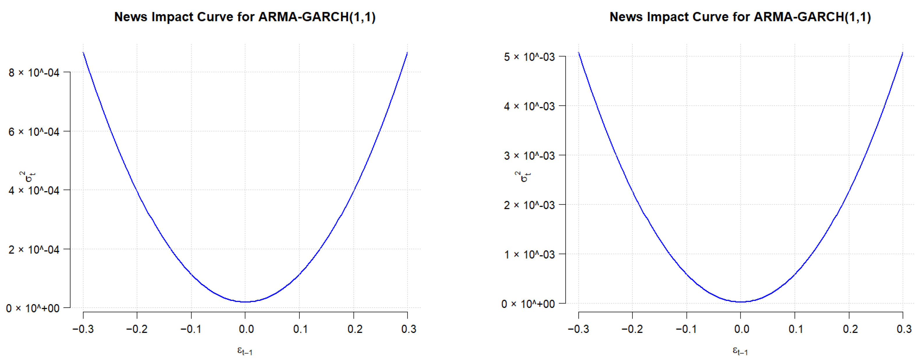
Figure A1. News impact curves for ARMA-GARCH(1,1) EURO/MRU exchange rate (first period on the (left), COVID-19 period on the (right)).
Jrfm 18 00589 g0a1
Figure A2. News impact curves for ARMA-GARCH(1,1) USD/MRU exchange rate (first period on the (left), COVID-19 period on the (right)).
Jrfm 18 00589 g0a2
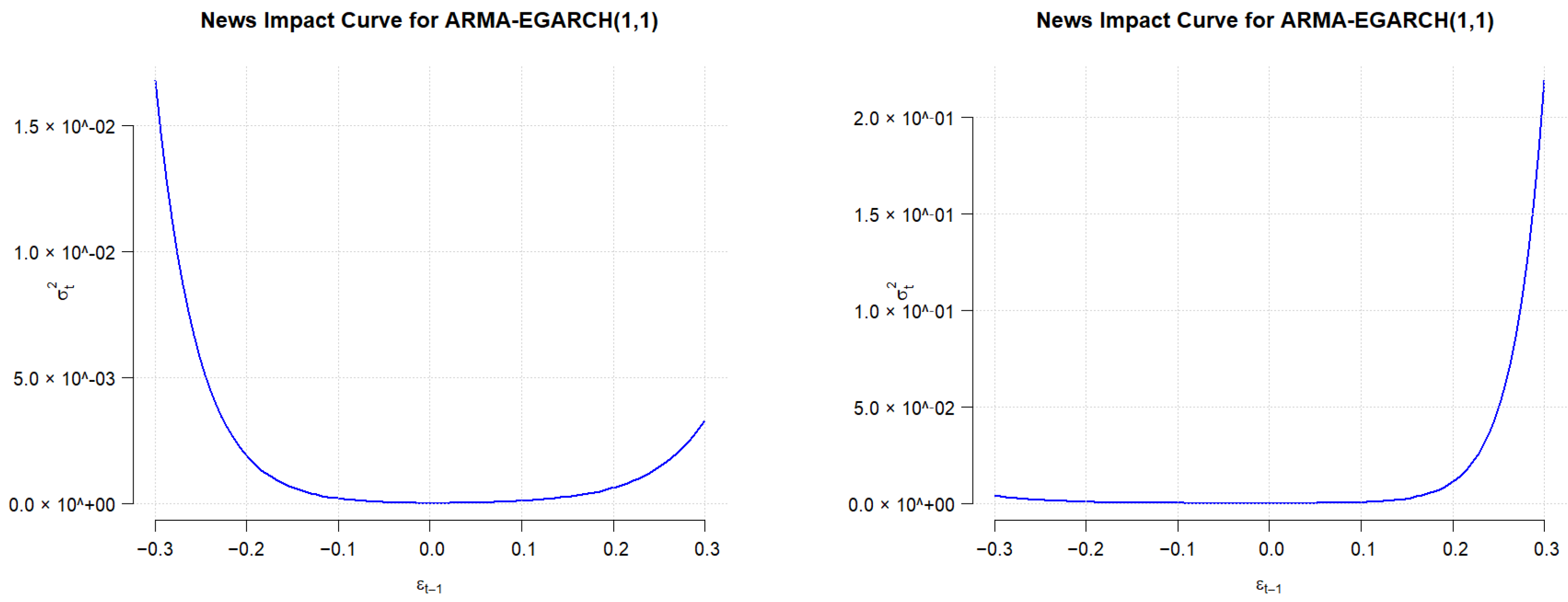
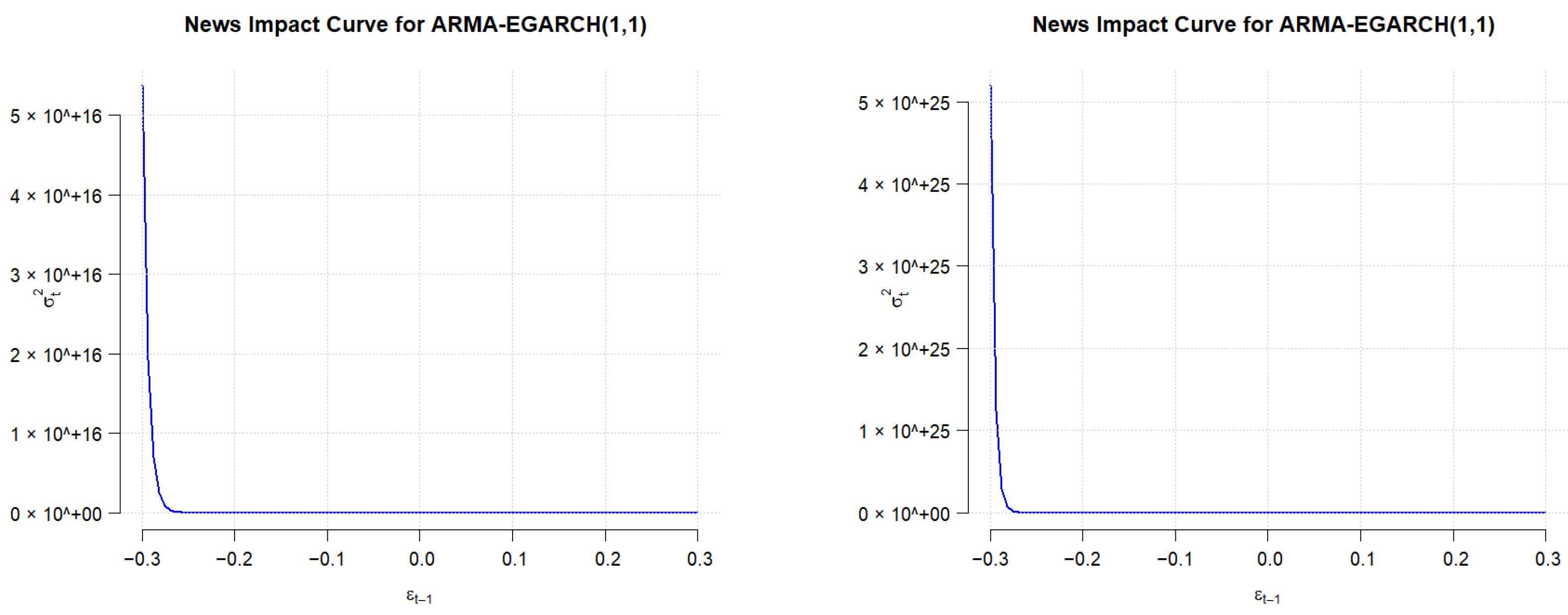
Figure A3. News Impact Curves for Exp-GARCH(1,1) EURO/MRU Exchange Rate (First Period on the (left), COVID-19 Period on the (right)).
Jrfm 18 00589 g0a3
Figure A4. News Impact Curves for Exp-GARCH(1,1) USD/MRU Exchange Rate (First Period on the (left), COVID-19 Period on the (right)).
Jrfm 18 00589 g0a4
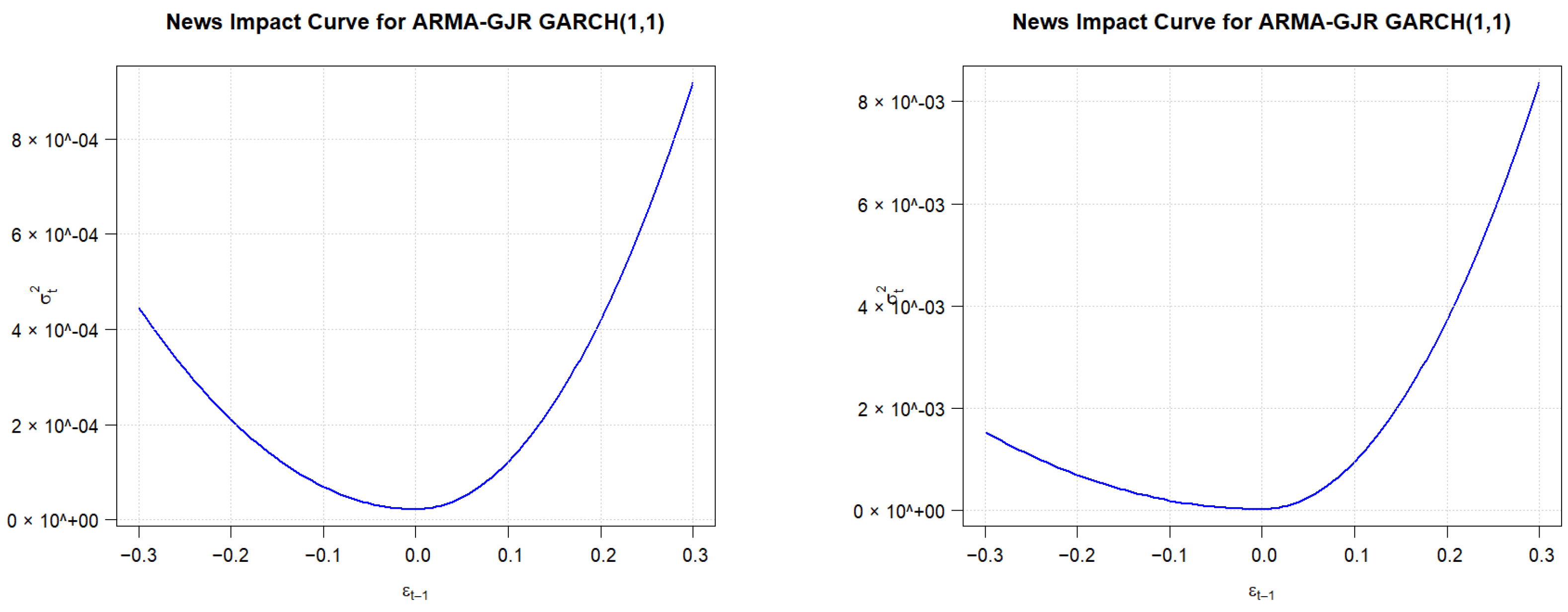
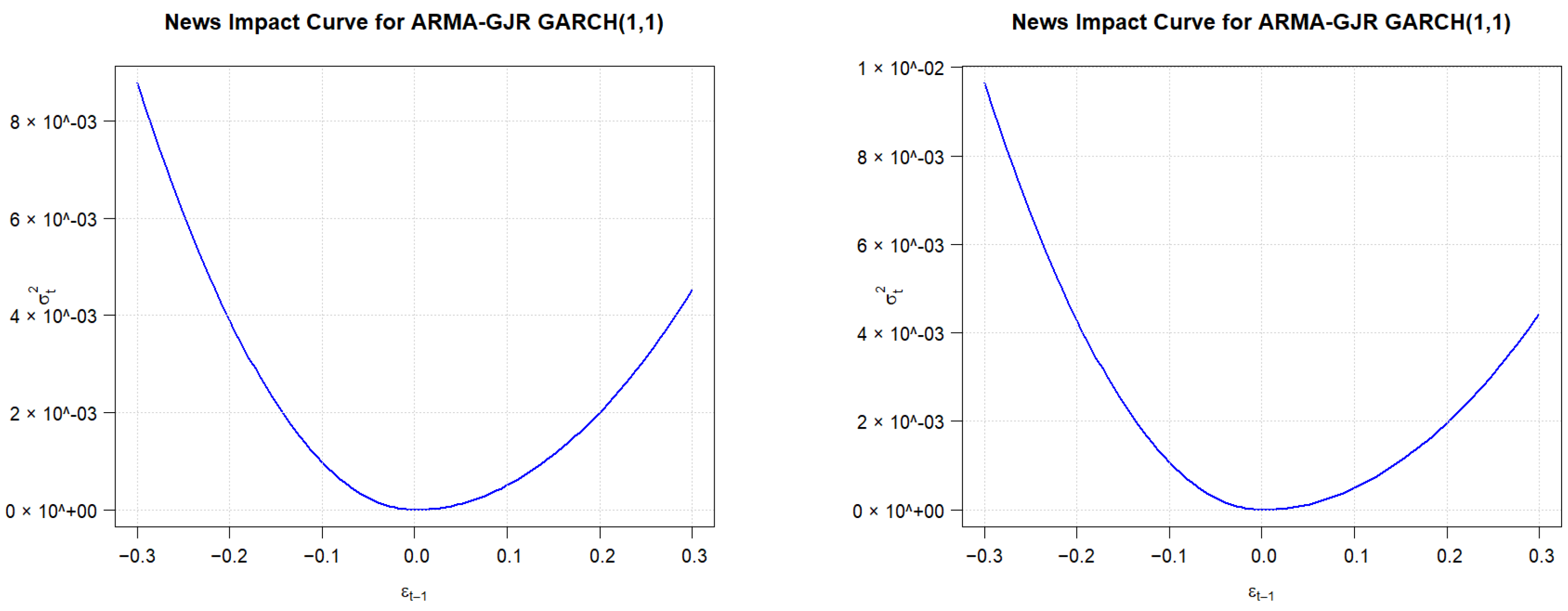
Figure A5. News impact curves for GJR-GARCH(1,1) EURO/MRU exchange rate (first period on the (left), COVID-19 period on the (right)).
Jrfm 18 00589 g0a5
Figure A6. News impact curves for GJR-GARCH(1,1) USD/MRU exchange rate (first period on the (left), COVID-19 period on the (right)).
Jrfm 18 00589 g0a6

References

  1. Benzid, L. (2020). The impact of COVID-19 on exchange rate volatility: Evidence through GARCH model. King Faisal University (KFU). [Google Scholar]
  2. Chen, X. (2023, April 15–16). Comparing various GARCH-type models in the estimation and forecasts of volatility of SP 500 returns during global finance crisis of 2008 and COVID-19 financial crisis [Article Number 01077]. 4th International Symposium on Frontiers of Economics and Management Science (FEMS 2023), Macao, China. [Google Scholar]
  3. Christoffersen. (2012). Elements of financial risk management. Christoffersen. [Google Scholar]
  4. Ciftci, C., & Durusu-Ciftci, D. (2021). Economic freedom, foreign direct investment, and economic growth: The role of sub-components of freedom. The Journal of International Trade & Economic Development, 31(2), 233–254. [Google Scholar] [CrossRef]
  5. Congressional Research Service (CRS). (2021). Global economic effects of COVID-19. CRS. [Google Scholar]
  6. Cook, A. R., Choi, K. P., & Wong, W. K. (2021). Contribution to the first discussion meeting on statistical aspects of the COVID-19 pandemic. Journal of the Royal Statistical Society. Series A, Statistics in Society, 185(4), 1826–1827. [Google Scholar] [CrossRef]
  7. Diebold, F. X., & Mariano, R. S. (1995). Comparing predictive accuracy. Journal of Business & Economic Statistics, 13(3), 253–263. [Google Scholar] [CrossRef] [PubMed]
  8. Dritsaki, C. (2019). Modeling the volatility of exchange rate currency using GARCH model. International Economics/Economia Internazionale, 72(2), 209–230. [Google Scholar]
  9. Endri, E., Aipama, W., Razak, A., Sari, L., & Septiano, R. (2021). Stock price volatility during the COVID-19 pandemic: The GARCH model. Investment Management & Financial Innovations, 18(4), 12–20. [Google Scholar]
  10. Enumah, N. K., & Adewinbi, H. S. (2022). An analysis of the exchange rate volatility in Poland using the GARCH, GJR-GARCH and EGARCH models. Earthline Journal of Mathematical Sciences, 11(2), 287–302. [Google Scholar] [CrossRef]
  11. Epaphra, M. (2017). Modelling exchange rate volatility: Application of the GARCH and EGARCH models. Journal of Mathematical Finance, 7, 121–143. [Google Scholar] [CrossRef]
  12. Ghosh, S. (2020). Predictive model with analysis of the initial spread of COVID-19 in India. International Journal of Medical Informatics, 143, 104262. [Google Scholar] [CrossRef] [PubMed]
  13. Hsieh, D. A. (1989). Modeling heteroscedasticity in daily foreign-exchange rates. Journal of Business & Economic Statistics, 7(3), 307–317. [Google Scholar] [PubMed]
  14. International Monetary Fund (IMF). (2020). Islamic Republic of Mauritania: Request for disbursement under the rapid credit facility—Press release; Staff report; and Statement by the executive director for the Islamic Republic of Mauritania (IMF country report No. 20/140). Available online: https://www.imf.org/en/Publications/CR/Issues/2020/04/23/Islamic-Republic-of-Mauritania-Request-for-Disbursement-Under-the-Rapid-Credit-Facility-Press-49347 (accessed on 5 October 2025).
  15. McKibbin, W., & Fernando, R. (2020). The global macroeconomic impacts of COVID-19: Seven scenarios. CAMA Working Paper No. 19/2020. Centre for Applied Macroeconomic Analysis, Australian National University. [Google Scholar]
  16. Ministry of Commerce and Tourism. (2022). Economic situation of Mauritania. Available online: https://www.mauritaniatrade.com/acheter-en-mauritanie/situation-economique-de-la-mauritanie.html (accessed on 5 October 2025).
  17. Patton, A. J. (2011). Volatility forecast comparison using imperfect volatility proxies. Journal of Econometrics, 160(1), 246–256. [Google Scholar] [CrossRef]
  18. Thuy, V. N. T., & Thuy, D. T. T. (2019). The impact of exchange rate volatility on exports in Vietnam: A bounds testing approach. Journal of Risk and Financial Management, 12(1), 6. [Google Scholar] [CrossRef]
  19. Wang, Y., Xiang, Y., Lei, X., & Zhou, Y. (2021). Volatility analysis based on GARCH-type models: Evidence from the Chinese stock market. Research-Ekonomska Istraživanja, 35(1), 2530–2554. [Google Scholar] [CrossRef]
  20. World Bank. (2020). Report on the economic situation in Mauritania 2022. Available online: https://www.worldbank.org/en/country/mauritania/publication/afw-mauritania-economic-update-2022-the-private-sector-at-the-centre-of-economic-transformation-and-job-creation (accessed on 5 October 2025).
  21. World Health Organization (WHO). (2020). Coronavirus disease (COVID-19) pandemic. Available online: https://www.who.int/emergencies/diseases/novel-coronavirus-2019 (accessed on 5 October 2025).
  22. Yunusa, L. A. (2020). Exchange rate volatility and Nigeria crude oil export market. Scientific African, 9, e00538. [Google Scholar] [CrossRef]
Figure 1. EURO/MRU first period exchange rate.
Jrfm 18 00589 g001
Figure 2. EURO/MRU COVID-19 period exchange rate.
Jrfm 18 00589 g002
Figure 3. USD/MRU first period exchange rate.
Jrfm 18 00589 g003
Figure 4. USD/MRU COVID-19 period exchange rate.
Jrfm 18 00589 g004
Figure 5. EURO/MRU return COVID-19 period.
Jrfm 18 00589 g005
Figure 6. USD/MRU return COVID-19 period.
Jrfm 18 00589 g006
Table 1. Descriptive statistics EURO/MRU—first period.
ReturnSquared Return
Mean0.00014290.0000260
Variance0.00002680.0000000
Std. Dev.0.00518330.0000575
Skewness−0.22888346.6819970
Kurtosis2.614533067.8760000
Table 2. Descriptive statistics EURO/MRU—COVID-19 period.
ReturnSquared Return
Mean0.0000700.000030
Variance0.00003090.000000
Std. Dev.0.0055580.000086
Skewness−0.60593913.534200
Kurtosis5.874297288.134400
Table 3. Descriptive statistics USD/MRU—first period.
ReturnSquared Return
Mean0.00004700.0000082
Variance0.00000820.0000000
Std. Dev.0.00280000.0000350
Skewness−0.760000010.2000000
Kurtosis16.9100000141.9800000
Table 4. Descriptive statistics USD/MRU—COVID-19 period.
ReturnSquared Return
Mean0.0000190.0000120
Variance0.0000120.0000000
Std. Dev.0.0034720.0000675
Skewness−1.73006218.8585700
Kurtosis29.431840498.5784000
Table 5. ADF test results for EUR/MRU during the first period and COVID-19 period.
ADF Test EURO/MRU
First PeriodCOVID-19 Period
Dickey-Fuller = −9.48Dickey-Fuller = −12.127
Lag order = 9Lag order = 10
p-value = 0.01p-value = 0.01
Table 6. ADF test results for USD/MRU during the first period and COVID-19 period.
ADF Test USD/MRU
First PeriodCOVID-19 Period
Dickey-Fuller = −11.13Dickey-Fuller = −12.27
Lag order = 9Lag order = 10
p-value = 0.01p-value = 0.01
Table 7. Autocorrelation test results for EURO/MRU.
Autocorrelation Test EURO/MRU
First PeriodCOVID-19 Period
X-squared = 58.273X-squared = 70.399
df = 20df = 20
p-value = 1.313 × 10 5 p-value = 1.567 × 10 7
Table 8. Autocorrelation test results.
Autocorrelation Test
First PeriodCOVID-19 Period
X-squared = 172.42X-squared = 222.83
df = 20df = 20
p-value < 2.2 × 10 16 p-value < 2.2 × 10 16
Table 9. Comparison of ARMA models for EUR/MRU and USD/MRU returns.
ModelEUR/MRU (AIC)USD/MRU (AIC)
ARMA(1,0)−6012.697−9017.753
ARMA(0,1)−6017.997−9069.294
ARMA(1,1)−6017.997−9069.294
ARMA(1,2)−6019.070−9069.294
ARMA(2,1)−6021.034−9069.294
ARMA(2,2)−6021.034−9069.294
Table 10. ARMA-GARCH(1,1) estimation results for EURO/MRU—first period.
ParameterEstimateStd. Errort-Statisticp-Value
μ 0.0001340.0001331.0090.313
AR(1)0.1793930.1450331.2370.216
MA(1)−0.3932530.134311−2.9280.003
ω 0.0000000.0000000.1260.900
α 1 0.0094120.0012567.4910.000
β 1 0.9881640.001197825.4550.000
GARCH Model: sGARCH(1,1); Mean Model: ARFIMA(1,0,1); Distribution: Normal.
Table 11. ARMA-GARCH(1,1) estimation results for EURO/MRU—COVID-19 period.
ParameterEstimateStd. Errort-Statisticp-Value
μ 0.0000730.0001180.6220.534
AR(1)−0.0188550.152368−0.1240.902
MA(1)−0.1709970.149756−1.1420.254
ω 0.0000020.00000021.3410.000
α 1 0.0561200.00420913.3340.000
β 1 0.8652150.00934392.6110.000
GARCH Model: sGARCH(1,1); Mean Model: ARFIMA(1,0,1); Distribution: Normal.
Table 12. ARMA-GARCH(1,1) estimation results for USD/MRU—first period.
ParameterEstimateStd. Errort-Statisticp-Value
μ −0.0002360.000031−7.6160.000
AR(1)0.0233570.0767110.3040.761
MA(1)−0.5706330.065121−8.7630.000
ω 0.0000000.0000000.0150.988
α 1 0.0615250.00182833.6550.000
β 1 0.9120220.0008071129.8770.000
GARCH Model: sGARCH(1,1); Mean Model: ARFIMA(1,0,1); Distribution: Normal.
Table 13. ARMA-GARCH(1,1) estimation results for USD/MRU—COVID-19 period.
ParameterEstimateStd. Errort-Statisticp-Value
μ −0.0000600.000114−0.5280.598
AR(1)−0.0446380.011502−3.8810.0001
MA(1)−0.4798050.011594−41.3850.000
ω 0.0000000.0000000.0420.966
α 1 0.0546510.000091601.3520.000
β 1 0.9193280.000949969.1640.000
GARCH Model: sGARCH(1,1); Mean Model: ARFIMA(1,0,1); Distribution: Normal.
Table 14. Differences in GARCH parameters between the first period and COVID-19 period for EURO/MRU.
Differences Between the Two Periods—EURO/MRU
ParameterDifference in ValueDifference in Percentage
μ 0.00−46%
AR(1)−0.20−111%
MA(1)0.22−57%
ω 0.00-
α 1 0.05496%
β 1 −0.12−12%
Table 15. Differences in GARCH parameters between the first period and COVID-19 period for USD/MRU.
Differences Between the Two Periods—USD/MRU
ParameterDifference in ValueDifference in Percentage
μ 0.0002−75%
AR(1)−0.0680−291%
MA(1)0.0908−16%
ω 0.00-
α 1 −0.0069−11%
β 1 0.00730.8%
Table 16. ARMA-eGARCH(1,1) estimation results for EURO/MRU—first period.
ParameterEstimateStd. Errort-Statisticp-Value
μ 0.0001190.0000901.3120.189
AR(1)0.1744060.0906991.9230.054
MA(1)−0.3556030.084394−4.2140.000
ω −0.5717260.013680−41.7930.000
α 1 −0.0140400.022524−0.6230.533
β 1 0.9456580.001527619.3320.000
γ 1 0.0986870.0126097.8270.000
GARCH Model: eGARCH(1,1); Mean Model: ARFIMA(1,0,1); Distribution: Normal.
Table 17. ARMA-eGARCH(1,1) estimation results for EURO/MRU—COVID-19 period.
ParameterEstimateStd. Errort-Statisticp-Value
μ 0.0001100.0000781.4140.157
AR(1)−0.0107430.008991−1.1950.232
MA(1)−0.1780680.021441−8.3050.000
ω −0.5705190.009694−58.8540.000
α 1 0.0384910.0178092.1610.031
β 1 0.9446950.001259750.5580.000
γ 1 0.1322330.01188711.1240.000
GARCH Model: eGARCH(1,1); Mean Model: ARFIMA(1,0,1); Distribution: Normal.
Table 18. ARMA-GJR-GARCH(1,1) estimation results for EURO/MRU—first period.
ParameterEstimateStd. Errort-Statisticp-Value
μ 0.0001400.0001331.0530.292
AR(1)0.1711470.1413891.2100.226
MA(1)−0.3897760.131776−2.9580.003
ω 0.0000000.0000000.1960.845
α 1 0.0099520.0042902.3200.020
β 1 0.9896290.0008971103.7530.000
γ 1 −0.0052530.007354−0.7140.475
GARCH Model: GJR-GARCH(1,1); Mean Model: ARFIMA(1,0,1); Distribution: Normal.
Table 19. ARMA-GJR-GARCH(1,1) estimation results for EURO/MRU—COVID-19 period.
ParameterEstimateStd. Errort-Statisticp-Value
μ 0.0001260.0001181.064390.287150
AR(1)0.0166660.1660750.100350.920066
MA(1)−0.2044690.162333−1.259560.207828
ω 0.0000020.00000012.723410.958
α 1 0.0926270.0170335.438160.000
β 1 0.8852500.008591103.041380.000
γ 1 −0.0758780.023498−3.229120.001242
GARCH Model: GJR-GARCH(1,1); Mean Model: ARFIMA(1,0,1); Distribution: Normal.
Table 20. Differences in E-GARCH parameters between the first period and COVID-19 period.
Differences Between the Two Periods—E-GARCH
ParameterDifference in ValueDifference in Percentage
μ 0.00−8%
AR(1)−0.19−106%
MA(1)0.18−50%
ω 0.000%
α 1 0.05374%
β 1 0.00−0.10%
γ 1 0.0334%
Table 21. Differences in GJR-GARCH parameters between the first period and COVID-19 period.
Differences Between the Two Periods—GJR-GARCH
ParameterDifference in ValueDifference in Percentage
μ 0.00−10%
AR(1)−0.154−90%
MA(1)0.185−48%
ω 0.0000%
α 1 0.083831%
β 1 −0.104−11%
γ 1 −0.0711344%
Table 22. ARMA-eGARCH(1,1) estimation results for USD/MRU—first period.
ParameterEstimateStd. Errort-Statisticp-Value
μ 0.0000790.0000243.3760.001
AR(1)0.1128760.0395012.8580.004
MA(1)−0.6403060.029439−21.7500.000
ω −5.7552871.100955−5.2280.000
α 1 −0.0675240.042492−1.5890.112
β 1 0.5144000.0922045.5790.000
γ 1 0.3834080.0629586.0900.000
GARCH Model: eGARCH(1,1); Mean Model: ARFIMA(1,0,1); Distribution: Normal.
Table 23. ARMA-eGARCH(1,1) estimation results for USD/MRU—COVID-19 period.
ParameterEstimateStd. Errort-Statisticp-Value
μ 0.0000570.0000105.8940.000
AR(1)−0.0309640.022751−1.3610.174
MA(1)−0.6243680.021336−29.2640.000
ω −3.9817370.340445−11.6960.000
α 1 −0.2281070.032879−6.9380.000
β 1 0.6469890.02942921.9850.000
γ 1 0.6127760.04824012.7030.000
GARCH Model: eGARCH(1,1); Mean Model: ARFIMA(1,0,1); Distribution: Normal.
Table 24. ARMA-GJR-GARCH(1,1) estimation results for USD/MRU—first period.
ParameterEstimateStd. Errort-Statisticp-Value
μ 0.0002630.0000003448.50.000
AR(1)0.0745210.0000213477.80.000
MA(1)−0.5527120.000161−3428.00.000
ω 0.0000000.0000000.0300.976
α 1 0.0501360.0000143466.90.000
β 1 0.9012580.0002773255.10.000
γ 1 0.0473540.0000143470.10.000
GARCH Model: GJR-GARCH(1,1); Mean Model: ARFIMA(1,0,1); Distribution: Normal.
Table 25. ARMA-GJR-GARCH(1,1) estimation results for USD/MRU—COVID-19 period.
ParameterEstimateStd. Errort-Statisticp-Value
μ 0.0002330.0000003474.40.000
AR(1)−0.065260.000019−3498.20.000
MA(1)−0.4804040.000139−3465.60.000
ω 0.0000000.0000000.051290.9583
α 1 0.0491590.0000143487.80.000
β 1 0.8988340.0002753267.40.000
γ 1 0.0580010.0000173489.00.000
GARCH Model: GJR-GARCH(1,1); Mean Model: ARFIMA(1,0,1); Distribution: Normal.
Table 26. Difference between the two periods for e-GARCH.
Difference Between the Two Periods (E-GARCH)
ParameterDifference in ValueDifference in %
μ −0.00002−29%
AR(1)−0.14384−127%
MA(1)0.015938−2%
ω 1.77−31%
α 1 −0.160583238%
β 1 0.13258926%
γ 1 0.22936860%
Table 27. Difference between the two periods for GJR-GARCH.
Difference Between the Two Periods (GJR-GARCH)
ParameterDifference in ValueDifference in %
μ −0.000027−10%
AR(1)−0.140−188%
MA(1)0.07213%
ω 0.000-
α 1 −0.001−2%
β 1 −0.0020%
γ 1 0.01122%
Table 28. Out-of-sample forecast evaluation results for EUR/MRU (COVID-19 period).
Loss FunctionARMA–GARCH(1,1)ARMA–GJR–GARCH(1,1)ARMA–EGARCH(1,1)
MSE 2.25 × 10 8 2.25 × 10 8 2.20 × 10 8
QLIKE1.8291.815 1.771
MAE-LOG1.7881.792 1.771
Table 29. Diebold–Mariano test results for EUR/MRU (COVID-19 period).
Model Comparison (A vs. B)DM Statisticp-Value
EGARCH vs. GARCH0.6660.506
GJR–GARCH vs. GARCH1.0850.279
EGARCH vs. GJR–GARCH0.5730.567
Table 30. Out-of-sample forecast evaluation results for USD/MRU (COVID-19 period).
Loss FunctionARMA–GARCH(1,1)ARMA–GJR–GARCH(1,1)ARMA–EGARCH(1,1)
MSE 5.5326 × 10 10 5.2091 × 10 10 5.2499 × 10 10
QLIKE3.4875 3.1103 3.2355
MAE-LOG3.4378 3.3737 3.5931
Table 31. Diebold–Mariano test results for USD/MRU (COVID-19 period).
Model Comparison (A vs. B)DM Statisticp-Value
EGARCH vs. GARCH1.2080.228
GJR–GARCH vs. GARCH−0.6630.508
EGARCH vs. GJR–GARCH1.9660.050
Table 32. Comparison of selection criteria for different GARCH models of EURO/MRU—first period.
S-GARCH(1,1)E-GARCH(1,1)GJR-GARCH(1,1)
AIC−7.7204−7.7305−7.7191
BIC−7.6845−7.6887−7.6772
Table 33. Comparison of selection criteria for different GARCH models of EURO/MRU—second period (COVID-19).
S-GARCH(1,1)E-GARCH(1,1)GJR-GARCH(1,1)
AIC−7.6094−7.6163−7.6160
BIC−7.5855−7.5885−7.5882
Table 34. Comparison of selection criteria for different GARCH models of USD/MRU—first period.
CriterionS-GARCH(1,1)E-GARCH(1,1)GJR-GARCH(1,1)
AIC−8.8556−9.2184−8.8818
BIC−8.8262−9.1840−8.8474
Table 35. Comparison of selection criteria for different GARCH models of USD/MRU—second period (COVID-19).
CriterionS-GARCH(1,1)E-GARCH(1,1)GJR-GARCH(1,1)
AIC−8.7659−8.9426−8.3973
BIC−8.7447−8.9179−8.3726
Disclaimer/Publisher’s Note: The statements, opinions and data contained in all publications are solely those of the individual author(s) and contributor(s) and not of MDPI and/or the editor(s). MDPI and/or the editor(s) disclaim responsibility for any injury to people or property resulting from any ideas, methods, instructions or products referred to in the content.