Deep Learning-Based Hybrid Model with Multi-Head Attention for Multi-Horizon Stock Price Prediction

Abstract

The prediction of stock prices is challenging due to their volatility, irregular patterns, and complex time-series structure. Reliably forecasting stock market data plays a crucial role in minimizing financial risk and optimizing investment strategies. However, traditional models often struggle to capture temporal dependencies and extract relevant features from noisy inputs, which limits their predictive performance. To improve this, we developed an enhanced recursive feature elimination (RFE) method that blends the importance of impurity-based features from random forest and gradient boosting models with Kendall tau correlation analysis, and we applied SHapley Additive exPlanations (SHAP) analysis to externally validate the reliability of the selected features. This approach leads to more consistent and reliable feature selection for short-term stock prediction over 1-, 3-, and 7-day intervals. The proposed deep learning (DL) architecture integrates a temporal convolutional network (TCN) for long-term pattern recognition, a gated recurrent unit (GRU) for sequence capture, and multi-head attention (MHA) for focusing on critical information, thereby achieving superior predictive performance. We evaluate the proposed approach using daily stock price data from three leading companies—HDFC Bank, Tata Consultancy Services (TCS), and Tesla—and two major stock indices: Nifty 50 and S&P 500. The performance of our model is compared against five benchmark models: temporal convolutional network (TCN), long short-term memory (LSTM), GRU, Bidirectional GRU, and a hybrid TCN–GRU model. Our method consistently shows lower error rates and higher predictive accuracy across all datasets, as measured by four commonly used performance metrics.

1. Introduction

Stock market forecasting is crucial in the financial sector, serving as the primary channel for corporate finance and a key indicator for investment decisions. Accurate stock price predictions enable investors to develop informed strategies, including determining when to buy, hold, or sell stocks and participating in futures trading and other financial assets, helping them manage risks and maximize returns (Naeem et al., 2024). Beyond its practical applications, stock price forecasting is a vital area of research in finance, economics, and related fields. It provides profound insights into financial market behavior and dynamics, shaping decision-making processes and strategies. However, stock price data, being a time series, frequently exhibit noise, dynamics, and nonlinearity, which pose challenges to accurate modeling and require sophisticated analytical techniques. To address these complexities, it is crucial to implement effective feature extraction methods and advanced nonlinear forecasting models to reveal market patterns, improve forecast accuracy, and reduce financial risks.

For decades, traditional statistical models like Autoregressive Integrated Moving Average (ARIMA) (Sirisha et al., 2022) and Generalized Autoregressive Conditional Heteroskedasticity (GARCH) (Caiado & Lúcio, 2023) have been the foundation of financial time-series forecasting. However, their dependence on linear assumptions restricts their ability to capture the complex nonlinear relationships in stock price movements accurately. To overcome this limitation, machine learning (ML) methods have been employed to capture complex nonlinear patterns, making them valuable for financial decision-making. Recently, deep learning (DL) models have outperformed traditional ML methods in tasks such as natural language processing, time-series analysis, and computer vision (Kanwal et al., 2022; Parray et al., 2020). In finance, they are increasingly used for stock and index prediction, portfolio optimization, risk management, and trading, thanks to their ability to automatically extract complex nonlinear patterns from financial time series.

Despite these advances, widely used algorithms, such as random forests, decision trees, neural networks, and support vector machines, often do not capture time-dependent patterns, reducing the accuracy of the forecast. DL frameworks such as temporal convolutional networks (TCNs), long-short-term memory (LSTM), convolutional neural networks (CNNs), and gated recurrent units (GRUs) address this challenge by recognizing intricate temporal dynamics and hierarchical feature representations, making them more effective for financial market prediction. Hybrid models that combine recurrent, convolutional, and attention-based architectures generally achieve more robust and precise forecasts than single-model approaches (Khodaee et al., 2022; Lei et al., 2020).

Although progress has been made in this field, key challenges remain. Feature selection is often inadequate, and large, noisy financial datasets can hinder model performance or lead to overfitting. In addition, many models focus on a single forecast horizon, usually the next day, while investors require accurate predictions over multiple time periods to guide trading and risk management. To address these limitations, a hybrid DL framework with effective feature selection is needed to provide reliable multi-horizon stock price forecasts.

Building upon the potential of hybrid DL frameworks, we introduce TCN-GRU-multihead attention (MHA), a novel approach to precise short-term stock price prediction over multiple time intervals (1-day, 3-day, and 7-day intervals). The TCN captures long-range dependencies and enhances generalization through causal and dilated convolutions. The GRU efficiently models sequential patterns in time-series data. Meanwhile, the MHA mechanism improves feature representation by assigning dynamic attention weights, allowing the model to focus on the most informative elements of the input. This study not only forecasts market closing prices across different time horizons but also integrates a robust feature selection strategy to identify the most influential predictors. The key contributions of this research study are the following:

(i)

A hybrid feature selection approach that combines nonparametric correlation analysis with recursive feature elimination to identify informative and non-redundant features, enhancing model performance.

(ii)

A novel integration of TCNs with GRUs and MHA allows the model to identify long-range dependencies, sequential dynamics, and diverse feature representations.

(iii)

Demonstration of the superior predictive accuracy of the proposed model, TCN-GRU-MHA, compared with traditional short-term stock price forecasting methods across multiple horizons (1-day, 3-day, and 7-day).

(iv)

To ensure sectoral diversity and comprehensive evaluation, we analyzed three stocks from different sectors and two major indices for evaluation.

The remainder of this article is arranged as follows: Section 2 presents related work and emphasizes key studies that inform and motivate our research. Section 3 presents the methodology, beginning with an overview of sequence modeling techniques, including the TCN, GRU, and MHA mechanisms. Then, the proposed model is introduced, followed by descriptions of the dataset, feature selection methods, and evaluation metrics. Section 4 presents and discusses the experimental findings, including comparisons with baseline and benchmark models. The results are summarized in Section 5, which also provides potential future directions.

2. Related Work

The continuous growth of financial markets underscores the importance of predicting stock prices. Several approaches have been developed to increase the accuracy of financial time-series forecasts, such as statistical methods, artificial intelligence methods, and hybrid methods (Chopra & Sharma, 2021). Researchers have implemented various methodologies and datasets to forecast stock prices. Initially, mathematical techniques such as residual analysis, parameter estimation, and curve fitting were frequently used to account for the non-linear character of stock market behavior.

2.1. Statistical Approaches

Traditional time-series methods such as ARIMA and GARCH have long been employed for financial forecasting. These models are grounded in rigorous mathematical principles that allow for precise parameter estimation and systematic model testing. For instance, Sirisha et al. (2022) applied ARIMA and seasonal autoregressive integrated moving average (SARIMA) models for profit forecasting, demonstrating the effectiveness of these statistical approaches in short-term time-series prediction. Similarly, Caiado and Lúcio (2023) proposed a clustering framework using forecast errors from asymmetric GARCH models to analyze the impact of COVID-19 on stock market behavior. Despite their historical relevance, these methods face critical limitations. They are heavily based on assumptions of linearity and stationarity, which restrict their ability to capture the highly nonlinear, volatile, and dynamic nature of financial markets. As a result, although ARIMA and GARCH remain standard tools in econometrics, their predictive performance is often inadequate for modern stock price forecasting, where complex temporal dependencies and nonlinear structures dominate.

2.2. Machine Learning and Deep Learning Approaches

In response to the limitations of statistical models, artificial intelligence (AI) methods have emerged as powerful alternatives to model nonlinear and non-stationary financial data (Chinta, 2021). Unlike ARIMA or GARCH, machine learning models eliminate the need for strict assumptions and extensive preprocessing, thereby offering greater flexibility in handling noisy and volatile markets. For example, Selvamuthu et al. (2019) applied support vector machines (SVMs) and artificial neural networks (ANNs) to forecast stock prices in the Indian market, where the integration of technical indicators within ANNs significantly improved prediction accuracy. Similarly, Gautam et al. (2024) demonstrated that LSTM-based models outperform linear forecasting techniques and ARIMA in capturing temporal dependencies of stock prices. Beyond traditional ML techniques such as random forests, decision trees, and SVMs, which often struggle to capture autocorrelation in sequential data, deep learning approaches have advanced financial forecasting considerably. DL architectures such as artificial neural networks (ANNs) (Atesongun & Gulsen, 2024), LSTM networks (Nourbakhsh & Habibi, 2023), gated recurrent units (GRUs) (Chi & Chu, 2021), convolutional neural networks (CNNs) (Hoseinzade & Haratizadeh, 2019), and temporal convolutional networks (TCNs) (Guo et al., 2023) have shown superior capabilities to model complex temporal structures. For example, Chen et al. (2023) introduced a GRU-based design that improved forecasting across multiple business sectors by efficiently capturing sequential dynamics, while Guo et al. (2023) highlighted the effectiveness of TCNs in long-range sequence modeling. Collectively, these studies underscore the transition from the traditional ML-based architecture to the DL-based architectures, which use hierarchical feature learning and temporal modeling to improve prediction accuracy in financial markets. However, challenges such as model complexity, computational cost, and risk of overfitting persist, motivating the exploration of hybrid and attention-based architectures.

2.3. Hybrid and Attention-Based Approaches

Several studies have demonstrated the effectiveness of hybrid DL models in improving stock price forecast accuracy by combining the strengths of different architectures. For instance, Khodaee et al. (2022) and Lei et al. (2020) highlighted that integrating recurrent, convolutional, and attention-based components enhances feature extraction and prediction performance. Francis Magloire Peujio Fozap (Fozap, 2025) applied a GRU–CNN hybrid model to the S&P 500 index and demonstrated that incorporating technical indicators boosted forecasting accuracy compared with traditional methods such as SVM, RF, and ARIMA. Expanding on this, Friday et al. (2024) integrated a GRU, a CNN, and AM for short-term trend prediction, where the AM module dynamically assigned weights to input sequences, allowing for the accurate detection of local and temporal dependencies. Similarly, Teixeira and Barbosa (2024) showed that the hybridization of a GRU and XGBoost, especially when combined with a CNN or an RNN, improved predictive performance under uncertain market conditions. Other researchers have introduced advanced attention-driven frameworks. Li et al. (2023) presented the AE-ACG model, where CNN–GRU layers extract features and an attention mechanism assigns weights to predict the close price. Yang et al. (2022) proposed the CNN–GRUA–FC model, which uses a random forest (RF) for feature selection before applying CNN and GRU modules augmented by attention, yielding enhanced accuracy. Likewise, Luo et al. (2024) combined a CNN, BiGRU, and AM to reduce information loss and improve stock correlation prediction. In parallel, TCNs have gained popularity for capturing long-range dependencies in time series. Zhou et al. (2022) proposed a TCN–GRU hybrid model for short-term bike-sharing demand prediction, effectively merging the TCN’s pattern extraction with the GRU’s sequential modeling. Xiaoyan et al. (2021) applied a similar TCN–GRU architecture for short-term load forecasting, demonstrating improved accuracy. In the financial domain, Jaiswal and Singh (2022) used a CNN–GRU model where 1D convolutions extracted features before the GRU layers modelled temporal dynamics. Additionally, Kervanci et al. (2024) optimized a GRU–GRU hybrid model using Bayesian methods, which outperformed conventional ML baselines.

Even with many advances in stock price forecasting, an important issue remains: selecting the most relevant features. Financial datasets often have many variables and can be noisy. Poor feature selection can reduce model performance and may lead to overfitting. Methods like recursive feature elimination (RFE) (Priyatno & Widiyaningtyas, 2024), filter-based techniques, and random forest feature importance have been used in other areas but are rarely applied with DL models for stock prediction. Most existing models focus on single-day forecasts, which are less useful for investors who need predictions over multiple horizons. To provide a structured overview of existing research, Table 1 summarizes selected studies related to stock price forecasting. It highlights the models employed, datasets used, key contributions, and identified limitations, offering a clear basis for understanding current progress and gaps in the literature.

Table 1. Summary of related work.

Reference	Method Used	Findings	Limitations
Sirisha et al. (2022)	ARIMA and SARIMA	Demonstrated effectiveness of ARIMA and SARIMA in modeling and forecasting financial profit time series.	Relies on linearity and stationarity assumptions; weak performance on nonlinear and volatile stock data.
Caiado and Lúcio (2023)	Asymmetric GARCH and clustering	Proposed error-clustering framework to evaluate asymmetric GARCH models under pandemic-driven volatility.	Limited ability to capture nonlinear and long-term dependencies; not scalable to complex datasets.
Kurani et al. (2023)	SVM	Comprehensive application of SVM in financial forecasting; effective in small and moderately nonlinear datasets.	Scalability issues with large datasets; weaker performance on highly volatile, nonlinear markets.
Guo et al. (2023)	TCN	Showed TCN’s ability to effectively model long-range sequence with parallel computation advantages.	Standalone TCN lacks temporal gating; may miss fine-grained sequential patterns.
Chen et al. (2023)	GRU	Demonstrated GRU’s efficiency in capturing temporal dynamics with fewer parameters than GRU.	Single-architecture focus; limited generalization across complex datasets.
Friday et al. (2024)	CNN-Attention-GRU	Conducted multi-horizon evaluation; dynamic weighting via attention improved robustness across markets.	Emphasis on short-term horizons; limited exploration of feature engineering depth.
Yang et al. (2022)	CNN–GRUA–FC and RF	Used RF for feature selection; CNN/GRU with attention improved sequential modeling.	High pipeline complexity; risk of overfitting on small datasets.
Li et al. (2023)	AE–ACG, CNN–GRU and Attention	Introduced autoencoder with CNN–GRU–attention to enhance feature extraction and prediction accuracy.	Shallow hybrid architecture; limited scalability to broader markets.
Luo et al. (2024)	CNN–BiGRU and Attention	Enhanced correlation forecasting by combining CNN, BiLSTM, and attention to reduce information loss.	Limited number of features; validation on a small set of stocks.

Motivated by recent developments in hybrid modeling strategies and the critical importance of feature selection, this paper introduces a novel model for stock price prediction, TCN-GRU-MHA. The model combines a TCN to extract key temporal patterns, a GRU to capture long-term dependencies in price movements, and MHA to dynamically assign importance to features, collectively improving predictive accuracy. Based on the complementary strengths of its components, the proposed model offers increased accuracy and robustness in forecasting. Unlike models that limit predictions to the next day, this framework generalizes across multiple short-term horizons, specifically 1-day, 3-day, and 7-day forecasts. This work enhances stock market prediction by utilizing hybrid architectures, effective feature extraction, and multi-horizon forecasting, thereby overcoming standard limitations in current approaches.

3. Methodology

This research study proposes a new model that combines a TCN, a GRU, and MHA to make stock market predictions more accurate and reliable. Before we discuss the proposed architecture, we provide a brief summary of each part: TCN, GRU, and MHA. This will help to understand how they fit into the overall design of the model.

3.1. Sequence Modeling Techniques

Sequence modeling approaches help us understand and forecast data that vary over time by finding patterns and connections between past and future values. Standard approaches to handling sequences include convolutional models such as TCNs, recurrent models like GRUs, and attention-based methods like MHA. Each of these works in a distinct yet effective manner.

3.1.1. Temporal Convolutional Networks

TCNs are deep learning models that are made especially for sequence modeling applications, such as natural language processing and time-series forecasting. They employ dilated causal convolutions to find both local and global relationships, making long-range temporal modeling more efficient.

In a TCN, the input sequence passes through convolutional layers, where each layer applies filters to extract relevant temporal patterns. Unlike traditional convolutional networks, TCNs use dilated convolutions, introducing fixed gaps between filter elements. By progressively increasing the dilation rate across layers (e.g., d = 1, 2, 4, 8), TCNs can capture dependencies over longer time horizons without incurring significant computational overhead. To enforce causality, padding is applied so that each output in a time step t depends only on inputs from time steps $\le t$, preventing information leakage from future inputs (Li et al., 2024). Figure 1 illustrates how dilated convolution expands the receptive field by increasing dilation rates across layers.

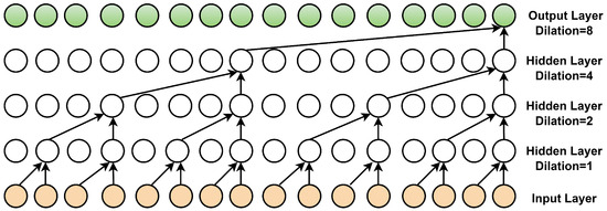
Figure 1. Structure of the dilated convolution.

A key component of TCNs is the residual module, which facilitates the training of deep networks. Figure 2 shows that each module begins with a dilated causal convolution that ensures that temporal order is preserved by restricting output to past inputs.

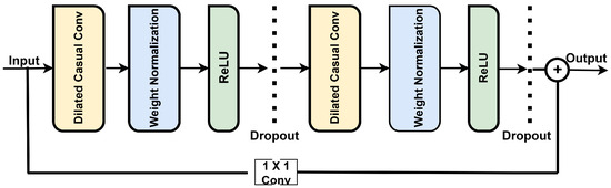
Figure 2. Structure of the residual module in the TCN.

Weight normalization scales the convolutional weights to stabilize and accelerate training, while a ReLU activation introduces nonlinearity for learning complex patterns. To reduce overfitting, a dropout layer randomly deactivates neurons during training. A residual connection, implemented through a $1\times 1$ convolution, allows the input to bypass the convolutional layers and be added to the output, mitigating vanishing gradients and allowing for deeper networks. These components collectively enhance the TCN’s ability to model long-range dependencies efficiently, making it well-suited for sequence modeling and time-series forecasting (Wen et al., 2024).

3.1.2. Gated Recurrent Unit

The proposed model utilizes a TCN to extract temporal features that capture long-term dependencies, which a GRU then processes to model sequential patterns essential to stock price prediction. Compared with LSTM networks, GRUs simplify the architecture by using only two gates, update and reset, thereby reducing computational complexity and training time (Salem, 2021). This model’s ability to retain $h_{t-1}$, the previous hidden state, is determined by the update gate $z_t$.

$$z_t=\sigma \left(W_z{x}_t+U_z{h}_{t-1}+b_z\right)$$

(1)

$W_z$ and $U_z$ are the weight matrices for the update gate applied to the input $x_t$ and the previous hidden state, $h_{t-1}$, respectively, while $b_z$ is the corresponding bias term. The function $\sigma (·)$ denotes the sigmoid activation function, which maps the values between 0 and 1. Before calculating the candidate hidden state, reset gate $r_t$ determines the amount of the previous hidden state, $h_{t-1}$, that the model discards. It is given by

$$r_t=\sigma \left(W_r{x}_t+U_r{h}_{t-1}+b_r\right)$$

(2)

The hidden state candidate, ${\tilde{h}}_t$, is calculated using reset gate $r_t$, where $W_r$ and $U_r$ represent the weight matrices and $b_r$ represents the bias term.

$${\tilde{h}}_t=tanh\left(W_h{x}_t+U_h\left(r_t\odot h_{t-1}\right)+b_h\right)$$

(3)

where the model uses $W_h$ and $U_h$ as weight matrices to calculate the candidate hidden state, applies $b_h$ as the bias term, and employs $tanh(·)$ as the hyperbolic tangent activation function. The term $r_t\odot h_{t-1}$ denotes the element-wise product, which selectively preserves portions of the previous hidden state based on the reset gate values. The model updates hidden state $h_t$ in time step t by blending the previous and candidate hidden states, weighted by update gate $z_t$.

$$h_t=(1-z_t)\odot h_{t-1}+z_t\odot {\tilde{h}}_t$$

(4)

where $(1-z_t)$ determines the proportion of $h_{t-1}$ to retain and $z_t$ controls the contribution of the hidden state candidate, ${\tilde{h}}_t$.

3.1.3. Multi-Head Attention Mechanism

The attention mechanism enables the model to focus on the most relevant features while reducing the impact of less important ones, thereby improving performance. To enhance this capability, the attention module operates in parallel through multiple attention heads, each learning different aspects of the input independently. To enable this, the module divides the query (Q), key (K), and value (V) parameters into N distinct parts. Each part is independently processed by a separate attention head, allowing the model to capture different contextual relationships within the input. The outputs from all heads are then concatenated and combined to produce the final output of attention (Luo et al., 2024; Wang & Peng, 2024). Figure 3 illustrates the architecture of the multi-head attention mechanism.

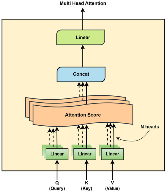
Figure 3. Detailed architecture of the multi-head attention layer.

To understand how attention weights are computed within this mechanism, consider a query vector q and an input sequence X. The probability of selecting the $i^{\mathrm{th}}$ input information ${\alpha }_i$ is defined by Equation (5):

$${\alpha }_i=p\left(z=i\mid H,q\right)=\mathrm{softmax}\left(s\left(x_i,q\right)\right)={\displaystyle \frac{e^{s\left(x,q\right)}}{{\sum }_{j=1}^N{e}^{s\left(x,q\right)}}}$$

(5)

In this context, z denotes the index position and the dimensions of the incoming data. $H=\left[\overleftrightarrow{h_1},\overleftrightarrow{h_2},\dots ,\overleftrightarrow{h_{\mathrm{N}}}\right]$ represents N, q denotes the query matrix, and $s\left(x_i,q\right)$ denotes the attention scoring function. The relevant formula is shown in Equation (6):

$$s\left(x_i,q\right)={\displaystyle \frac{x_i^{T}q}{\sqrt{d}}}$$

(6)

The dimension of the input information is denoted by d. Equation (7) is the scaled-dot product attention function that is employed:

$$\mathrm{Attention}\left(Q,K,V\right)=\mathrm{softmax}\left({\displaystyle \frac{Q{K}^T}{\sqrt{d_k}}}\right)V$$

(7)

where the query, key, and value matrices are denoted by Q, K, and V, respectively, and the dimension of the key vectors is $d_k$. The multi-head attention mechanism consists of multiple self-attention structures simultaneously processing the same feature information. Its output is the concatenation of the results of these numerous self-attention mechanisms. In this study, three attention mechanisms are concatenated, as shown in Figure 3. This structure enhances the model’s ability to capture dependencies between different features, improving its performance. The corresponding expression is given by Equation (8):

$$\mathrm{MultiHead}\left(Q,K,V\right)=\mathrm{Concat}\left({\mathrm{hd}}_1,{\mathrm{hd}}_2,\dots ,{\mathrm{hd}}_n\right)W^o$$

(8)

where ${\mathrm{hd}}_i=\mathrm{Attention}\left(Q{W}_i^Q,K{W}_i^K,V{W}_i^V\right),W_i^Q,W_i^K,W_i^V$ is the mapping matrix weight and $W^o$ is the output weight matrix.

3.2. Proposed Model

The proposed model, TCN-GRU-MHA, integrates a TCN, a GRU, and multi-head attention to effectively capture complex temporal dependencies in sequential data. The TCN extracts long-range features through dilated convolutions, which are then processed by the GRU to efficiently model sequential patterns. The MHA layer further enhances the model by attending to parallel parts of the sequence, capturing contextual relationships. The final output passes through fully connected layers for prediction. This integrated architecture, shown in Figure 4, is well-suited for time-series forecasting and sequence classification.

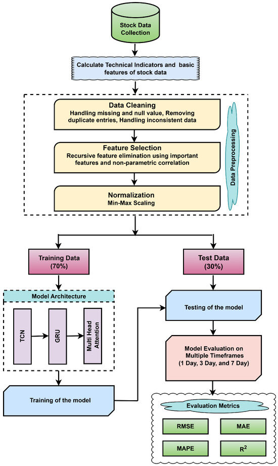
Figure 4. Architecture of the proposed model.

The figure illustrates the end-to-end workflow of the proposed stock price prediction framework. The process begins with collecting historical stock data and computing 36 features. These raw data are then subjected to cleaning and normalization to ensure consistency across features. Next, feature selection is performed using a combination of model-based importance scores and statistical correlation analysis. Specifically, feature importance is derived by averaging the scores from two ensemble learning models: the random forest (RF) regressor and the gradient boosting (GB) regressor. In parallel, Kendall tau correlation is employed to evaluate the statistical relationship between each feature and the target variable. Both sets of scores are scaled and combined using a weighted scheme assigning $75\%$ weight to the model-based scores and $25\%$ to the Kendall correlation scores. The resulting composite scores are used to identify the top 15 most relevant features, as detailed in Section 3.3.2. After preprocessing, the dataset is split into training ($70\%$) and test ($30\%$) subsets. The refined data are then fed into a hybrid DL model that integrates the TCN, the GRU, and MHA. This architecture effectively captures short-term fluctuations and long-term temporal dependencies in the time-series data. The model is trained and evaluated across multiple forecast horizons, specifically 1-day, 3-day, and 7-day intervals, using appropriate performance metrics to assess predictive accuracy.

3.3. Data Description, Preprocessing, and Feature Selection

3.3.1. Data Description

This study uses historical daily market data from leading companies across various sectors to establish a robust foundation for short-term stock price analysis. The dataset comprises daily stock prices from three major companies and two benchmark indices, chosen to ensure diversity across both geographies and industries. From the Indian market, we include Housing Development Finance Corporation Bank Ltd. (HDFC Bank, Mumbai, India), representing the banking sector, and Tata Consultancy Services (TCS, Mumbai, India) of the information technology sector. To capture an international perspective, we consider Tesla Inc. (TSLA), headquartered in Austin, Texas, USA, a multinational company in the automotive and clean energy sectors. In addition to individual stocks, we incorporate two benchmark indices to reflect broader market trends: Nifty 50, which tracks 50 large Indian companies across multiple sectors, and S&P 500, the primary USA index comprising 500 leading firms from diverse industries. The dataset covers the time from 1 January 2015 to 31 January 2025. A detailed description of the dataset is presented in Table 2.

Table 2. Detailed description of the stock dataset.

No.	Stock/Index	Sector/Country	Data Length	Mean	Max	Min	Std
1	HDFC Bank	Banking	2499	$1153.72$	$1871.75$	$470.28$	$395.47$
2	TCS	IT	2499	$2423.90$	$4553.75$	$1030.04$	$1046.00$
3	TSLA	Automotive	2536	$117.96$	$479.86$	9.58	$116.62$
4	Nifty 50	India	2500	13,590.09	26,216.05	$6970.60$	$5035.17$
5	S&P 500	USA	2536	$3376.81$	$6118.71$	$1829.10$	$1104.31$

These data provide a comprehensive view of market activity for HDFC Bank, TCS, TSLA, and two indices, Nifty 50 and S&P 500, delivering key insights into the performance and volatility of these stocks over time. Historical trends are the backbone for numerous stock prediction models, which rely on past trading patterns to anticipate future market movements.

3.3.2. Data Preprocessing and Feature Selection

The proposed approach augments the dataset by integrating 36 features, including 5 basic market features, i.e., Open, High, Low, Close, Volume; 19 commonly use TIs; and 12 derived indicators, i.e., HLC3, Mean HL, Rolling Mean5, Rolling Std5, Price Range, Upper Shadow, Lower Shadow, Candle Direction, Daily Return, Volatility, Normalized Volume, and Price Position Range. These intended features capture short-term market behavior and improve the model’s predictive abilities by identifying underlying structures and crucial temporal patterns for stock trend predictions. The included TIs encompass various categories and are commonly used in financial analysis, such as rate of change (ROC), momentum, true strength index (TSI), price rate of change (PROC), positive vortex indicator (VI+), mass index, parabolic stop and reverse (Parabolic SAR), on-balance volume (OBV), Chaikin money flow (CMF), triple exponential average (TRIX), simple moving average (SMA), exponential moving average (EMA), relative strength index (RSI), moving average convergence divergence (MACD), Bollinger bands (BB), average true range (ATR), commodity channel index (CCI), Williams %R, and stochastic oscillator (Stochastic). These comprehensive features collectively form a robust foundation for capturing complex market dynamics and significantly enhance the accuracy of time-series forecasting models (Mostafavi & Hooman, 2025; Teixeira & Barbosa, 2024).

This study used three different stock datasets and two indices. Among them, the HDFC Bank dataset was selected for visualization and feature importance analysis, as it exhibited correlation structures and feature importance rankings similar to the other datasets. Therefore, analyzing HDFC Bank alone was sufficient to reveal the underlying patterns in all datasets. Figure 5 represents the correlation heatmap of the parameters for the HDFC Bank dataset. The graphic illustrates the pairwise correlation coefficients among 36 features. Stronger positive correlations are shown in dark red, whereas strong negative correlations are shown in blue, facilitating the easy detection of linear connections among features.

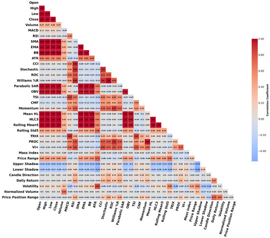
Figure 5. Correlation heatmap of selected financial features for the HDFC Bank dataset.

Feature selection began with an initial set of 36 features. Since the closing price served as the target variable, it was excluded from the input feature set, resulting in 35 features being used for selection. The importance of the feature was then evaluated using two ensemble learning models: the random forest (RF) and gradient boosting (GB) regressors. Both models utilize 100 estimators with a constant random state for reproducibility purposes. In the training phase, the models were trained on the dataset using $\mathrm{RF}·\mathrm{fit}(\mathrm{X},\mathrm{y})$ and $\mathrm{GB}·\mathrm{fit}(\mathrm{X},\mathrm{y})$, where X signifies the feature matrix and y indicates the target variable (closing price).

After training, the models generated feature importance scores, which were retrieved using $RF·\mathrm{Feature}\mathrm{Importance}$ and $GB·\mathrm{Feature}\mathrm{Importance}$. To produce a more stable and robust ranking, the process averaged the two sets of scores as follows:

$$\mathrm{Combined}\mathrm{Importance}={\displaystyle \frac{\mathrm{RF}·\mathrm{Feature}\mathrm{Importance}+\mathrm{GB}·\mathrm{Feature}\mathrm{Importance}}{2}}$$

(9)

The analysis used Kendall tau correlation to assess the statistical relationship between each selected feature and the target variable. It computed the correlation coefficients by iterating through all features and applying the following formula:

$${\tau }_{\mathrm{score}}=\mathrm{Kendall’s}\mathrm{Tau}(X_{\mathrm{feature}},y)$$

(10)

where $\tau$ represents the Kendall tau correlation coefficient, $X_{\mathrm{feature}}$ denotes the feature values, and y is the target variable. The analysis stored the absolute values of the correlation coefficients in Kendall scores. To ensure comparability between ML-based feature importance and statistical correlation, both metrics were normalized using MinMaxScaler, resulting in the scaled values. To integrate important features with Kendall correlation scores, three weighting strategies were evaluated: (1) $25\%$ feature importance and $75\%$ Kendall correlation scores, (2) an equal weighting of $50\%$ each, and (3) $75\%$ feature importance and $25\%$ Kendall correlation scores. Among these, the third strategy—comprising $75\%$ feature importance and $25\%$ Kendall correlation scores—demonstrated superior performance and was thus adopted as the final feature fusion approach.

$$\mathrm{Final}\mathrm{Weighted}\mathrm{Score}=0.75\times \mathrm{Combined}\mathrm{Importance}+0.25\times {\tau }_{\mathrm{score}}$$

(11)

After that, a combined importance score was used to rate each feature. This score was based on both model-based importance and correlation-based criteria. We applied a weighted formula to compute the final score. Features with the highest scores were selected, and the dataset was modified to retain only these top-performing features. Table 3 presents the descriptions and final weighted scores of all 35 features.

Table 3. Feature importance scores of the HDFC Bank dataset.

Rank	Feature	Description	Final Weighted Score
1	HLC3	Average of high, low, and close price	1.000000
2	Mean HL	Mean of High and Low	0.333048
3	Low	Lower price	0.311132
4	High	Higher price	0.281828
5	Open	Opening price	0.247799
6	Rolling Mean5	5-Period moving average	0.244660
7	Parabolic SAR	Parabolic stop and reverse	0.237286
8	EMA	Exponential moving average	0.236381
9	SMA	Simple moving average	0.233920
10	BB	Volatility bands around price average	0.229445
11	OBV	Cumulative volume flow indicator	0.207496
12	ATR	Volatility measurement over time	0.134234
13	Volume	Trading intensity over time	0.114961
14	Price Range	High–low-price difference	0.109802
15	Rolling Std5	5-Period rolling standard deviation	0.097434
16	Upper Shadow	Wick above candle body	0.065497
17	Lower Shadow	Wick below candle body	0.057736
18	MACD	Momentum and trend strength indicator	0.027607
19	Volatility	Measure of market fluctuation	0.026295
20	CMF	Money flow strength indicator	0.013079
21	Momentum	Speed of price movement	0.011721
22	TRIX	Filters short-term price noise	0.006090
23	Mass Index	Range expansion reversal indicator	0.003344
24	PROC	Measures price momentum shift	0.003286
25	Normalized Volume	Relative volume across time	0.003129
26	Candle Direction	Bullish or bearish candle signal	0.002402
27	Daily Return	Daily price return percentage	0.002206
28	ROC	Price momentum strength indicator	0.002105
29	Price Position Range	Price level in recent range	0.001361
30	CCI	Measures price deviation strength	0.000752
31	VI+	Positive vortex indicator	0.000300
32	Williams %R	Price position in recent range	0.000184
33	Stochastic	Measures price relative to range	0.000183
34	TSI	Identifies trend strength and direction	0.000163
35	RSI	Measures overbought or oversold	0.000001

According to the results, the forecasting model was limited to using only the 15 most important features. The final weighted score guided this decision, combining model-based feature importance and Kendall tau correlation to ensure statistical significance and relevance to the target variable. The top 15 selected features are HLC3, Mean HL, Low, High, Open, Rolling Mean5, Parabolic SAR, EMA, SMA, BB, OBV, ATR, Volume, Price Range, and Rolling Std5. These features comprehensively capture market dynamics, price behavior, and volatility patterns, forming a robust foundation for accurate stock trend forecasting.

To ensure the reliability of the proposed feature selection strategy, we conducted external validation using SHAP (SHapley Additive exPlanations) analysis. The top 15 features identified by our weighted scoring method were compared with those ranked the highest by SHAP values. The analysis indicated that 11 features were common to both approaches, demonstrating a strong level of agreement between the two methods. Retaining the most informative features reduces complexity, limits overfitting, and improves training efficiency without compromising accuracy. Figure 6 displays the SHAP-based importance scores of the best 15 features, highlighting their relative significance and contribution to the prediction model and guiding the feature selection process.

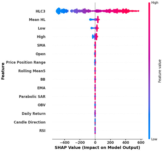
Figure 6. SHAP-based importance scores of the top 15 features.

3.4. Evaluation Metrics

This study uses commonly used regression metrics for evaluating models that predict stock prices, including root mean squared error (RMSE), mean absolute error (MAE), mean absolute percentage error (MAPE), and coefficient of determination (${\mathrm{R}}^2$). The square root of the mean squared discrepancies between actual values $y_i$ and their associated forecasts ${\widehat{y}}_i$, known as the RMSE, is used to estimate the average size of prediction mistakes (Sarıkoç & Celik, 2024).

$$\mathrm{RMSE}=\sqrt{{\displaystyle \frac{1}{n}}\sum _{i=1}^n{(y_i-{\widehat{y}}_i)}^2}$$

(12)

The MAE measures the overall magnitude of the absolute discrepancies between actual and predicted values, as defined below.

$$\mathrm{MAE}={\displaystyle \frac{1}{n}}\sum _{i=1}^n|y_i-{\widehat{y}}_i|$$

(13)

The MAPE quantifies the prediction error as a percentage of the actual values, providing a standardized measure of accuracy (14).

$$\mathrm{MAPE}={\displaystyle \frac{1}{n}}\sum _{i=1}^n\left|{\displaystyle \frac{y_i-{\widehat{y}}_i}{y_i}}\right|\times 100$$

(14)

${\mathrm{R}}^2$ quantifies the proportion of variance in the target variable that the model explains. A higher value of ${\mathrm{R}}^2$ indicates stronger predictive performance. The equation for ${\mathrm{R}}^2$ is given by

$${\mathrm{R}}^2=1-{\displaystyle \frac{{\sum }_{i=1}^n{(y_i-{\widehat{y}}_i)}^2}{{\sum }_{i=1}^n{(y_i-\overline{y})}^2}}$$

(15)

where $\overline{y}$ represents the mean of the actual values. These measurements quantify the difference between the model’s predictions and actual market values, offering critical insights into the accuracy and reliability of the forecasting models.

4. Results and Discussion

This section compares the efficacy of six DL models for short-term stock price forecasting: TCN, LSTM, GRU, BiGRU, TCN-GRU, and the proposed model, TCN-GRU-MHA. The assessment utilizes historical daily stock data from three large Indian corporations, namely, HDFC Bank, TCS, and HUL, over forecast periods of 1, 3, and 7 days. The analysis evaluates performance using four conventional metrics: RMSE, MAE, MAPE, and ${\mathrm{R}}^2$. All models are trained on the same dataset with identical hyperparameters for consistency.

The implementation uses ‘Python’ with ‘Keras API’ and a ‘TensorFlow’ backend, while the experiments are run on ‘Google Colab’ equipped with an Intel Xeon CPU and 16 GB of RAM. Selecting an optimal input time window is critical to effectively capturing temporal dependencies in time-series stock data. A very short step increases computational overhead and introduces noise, often leading to overfitting, while a very long step may overlook essential short-term fluctuations, reducing predictive accuracy. This study evaluated three input sequence lengths, 10, 20, and 30 days, to address this. Among these, the 20-day input window yielded the highest prediction accuracy for TCN-GRU-MHA. Consequently, this time step was adopted across all models in the study to ensure consistency and fairness in comparison.

The evaluation compared the proposed model with five benchmark architectures, TCN, LSTM, GRU, BiGRU, and TCN-GRU, under identical experimental conditions. Each model was trained for 100 epochs with a batch size of 32, and the dataset was split into $70\%$ for training and $30\%$ for testing. hyperparameters of the model were refined by a grid search methodology to achieve optimal performance. The optimized configuration for TCN-GRU-MHA, which includes the use of causal padding in the TCN layer, dual-layer GRUs with 128 and 64 units, an MHA mechanism with four filters and a key dimension of 16, and a ‘ReLU’ activation function, is presented in Table 4. The model employs the ‘Adam’ optimizer with a learning rate of $0.005$, with mean squared error (MSE) as the loss function. The model applies a dropout rate of $0.2$ to prevent overfitting and employs early stopping with a patience threshold of 10 to enhance generalization. These settings are consistently applied to all benchmark models to ensure balanced and rigorous comparison.

Table 4. Details of the parameters for TCN-GRU-MHA.

Parameter	Value
Number of TCN Filters	64
Kernel Size	3
Dilation Rate	[1, 2, 4, 8]
Padding	Causal
GRUs	128, 64
Number of Filters (MHA)	4
Key Dimension	16
Loss Function	MSE
Activation Function	ReLU
Optimizer	Adam
Batch Size	32
Dropout Rate	$0.2$
Epochs	100
Learning Rate	$0.005$
Early Stopping	patience = 10

4.1. Performance Evaluation on HDFC Bank Stock Data

We evaluate the proposed model, TCN-GRU-MHA, against baseline models—TCN, LSTM, GRU, BiGRU, and TCN-GRU—across different prediction horizons: 1 day, 3 days, and 7 days. Table 5 presents the evaluation results based on the metrics RMSE, MAE, MAPE, and ${\mathrm{R}}^2$, providing a comprehensive comparison of the models in terms of predictive accuracy and error reduction. In this work, RMSE, MAE, and MAPE are treated as scaled error measures, whereas ${\mathrm{R}}^2$ represents the actual performance outcome as it quantifies the proportion of variance explained by the model. For the 1-day forecast, the proposed model performs the best, with an RMSE of 0.014, an MAE of 0.008, an MAPE of 1.21%, and an ${\mathrm{R}}^2$ score of 0.981. These results show that the model is highly accurate in capturing short-term changes. The next best model, TCN-GRU, shows slightly higher errors and a lower ${\mathrm{R}}^2$ of 0.978, while traditional models such as LSTM and TCN perform less effectively. The 3-day forecast shows that the proposed model gives the best results, with an RMSE of 0.031, an MAE of 0.022, an MAPE of 2.40%, and a ${\mathrm{R}}^2$ of 0.948. This means that the model remains accurate for a longer period of time. TCN and LSTM, on the other hand, perform worse, with lower ${\mathrm{R}}^2$ scores (0.892 and 0.901) and higher error values. For the 7-day forecast, although the prediction uncertainty increases, the proposed model still leads, with an RMSE of 0.072, an MAE of 0.051, an MAPE of 5.10%, and an ${\mathrm{R}}^2$ of 0.849. Despite a slight drop in performance, it outperforms TCN-GRU (0.846) and GRU (0.834) and significantly surpasses TCN (0.803), confirming its robustness across varying forecast horizons.

Table 5. Summary of model performance in predicting HDFC stock prices over 1-day, 3-day, and 7-day time frames.

Time Frame	Model	RMSE	MAE	MAPE	R2
1 Day	TCN	$0.032$	$0.024$	$2.36\%$	$0.937$
	LSTM	$0.027$	$0.020$	$1.90\%$	$0.951$
	GRU	$0.025$	$0.018$	$1.82\%$	$0.956$
	BiGRU	$0.021$	$0.015$	$1.65\%$	$0.965$
	TCN-GRU	$0.017$	$0.011$	$1.43\%$	$0.978$
	Proposed Model	$0.014$	$0.008$	$1.21\%$	$0.981$
3 Days	TCN	$0.048$	$0.036$	$3.13\%$	$0.892$
	LSTM	$0.044$	$0.033$	$3.02\%$	$0.901$
	GRU	$0.042$	$0.032$	$2.93\%$	$0.907$
	BiGRU	$0.039$	$0.029$	$2.84\%$	$0.914$
	TCN-GRU	$0.034$	$0.025$	$2.61\%$	$0.933$
	Proposed Model	$0.031$	$0.022$	$2.40\%$	$0.948$
7 Days	TCN	$0.091$	$0.067$	$6.34\%$	$0.803$
	LSTM	$0.087$	$0.064$	$5.96\%$	$0.815$
	GRU	$0.078$	$0.057$	$5.45\%$	$0.834$
	BiGRU	$0.082$	$0.060$	$5.73\%$	$0.828$
	TCN-GRU	$0.074$	$0.053$	$5.21\%$	$0.846$
	Proposed Model	$0.072$	$0.051$	$5.10\%$	$0.849$

Figure 7 compares actual and predicted HDFC Bank stock prices using TCN, LSTM, GRU, BiGRU, TCN-GRU, and the proposed TCN-GRU-MHA model across different forecast horizons: (a) 1-day, (b) 3-day, and (c) 7-day. The x-axis shows the timeline in month-year format, and the y-axis shows the stock price in Indian Rupees (INR). The model is superior to baseline methods and is very similar to the real values. It does an excellent task of finding short-term patterns by using multi-head attention, which shows how adaptable and useful it is for predicting stock prices.

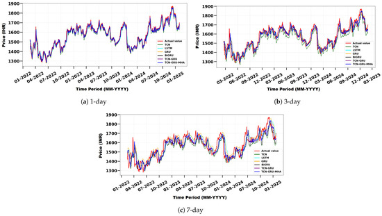
Figure 7. Comparison of actual and predicted HDFC Bank stock prices using TCN, LSTM, GRU, BiGRU, TCN-GRU, and the proposed model for different forecast horizons: (a) 1 day, (b) 3 days, and (c) 7 days.

4.2. Performance Evaluation on TCS Stock Data

The performance of the proposed model in predicting the prices of TCS stock is presented in Table 6. Across all prediction horizons (1 day, 3 days, and 7 days), the model consistently outperforms baseline architectures, including TCN, LSTM, GRU, BiGRU, and TCN-GRU, in terms of RMSE, MAE, MAPE, and ${\mathrm{R}}^2$ metrics. In the 1-day forecast, the proposed model achieves the lowest RMSE (0.072), MAE (0.050), and MAPE (1.44%), along with the highest ${\mathrm{R}}^2$ score (0.987), indicating strong short-term predictive capacity. On the 3-day horizon, it maintains superior performance, with an RMSE of 0.105 and an ${\mathrm{R}}^2$ of 0.964, outperforming all comparative models. Although error metrics increase slightly over the 7-day horizon, the proposed model remains the most accurate, recording an RMSE of 0.194, an MAPE of 6.43%, and an ${\mathrm{R}}^2$ value of 0.857. These results confirm the robustness and generalization capability of the model across short- to medium-term forecasting windows.

Table 6. Summary of model performance in predicting TCS stock prices over 1-day, 3-day, and 7-day time frames.

Time Frame	Model	RMSE	MAE	MAPE	R2
1 Day	TCN	$0.110$	$0.075$	$3.20\%$	$0.942$
	LSTM	$0.098$	$0.067$	$2.88\%$	$0.954$
	GRU	$0.089$	$0.060$	$2.45\%$	$0.967$
	BiGRU	$0.082$	$0.056$	$2.03\%$	$0.978$
	TCN-GRU	$0.077$	$0.053$	$1.70\%$	$0.981$
	Proposed Model	$0.072$	$0.050$	$1.44\%$	$0.987$
3 Days	TCN	$0.169$	$0.117$	$4.31\%$	$0.906$
	LSTM	$0.150$	$0.106$	$3.96\%$	$0.922$
	GRU	$0.126$	$0.093$	$3.32\%$	$0.953$
	BiGRU	$0.138$	$0.098$	$3.55\%$	$0.948$
	TCN-GRU	$0.112$	$0.087$	$3.12\%$	$0.959$
	Proposed Model	$0.105$	$0.082$	$2.91\%$	$0.964$
7 Days	TCN	$0.257$	$0.168$	$7.88\%$	$0.803$
	LSTM	$0.244$	$0.161$	$7.56\%$	$0.812$
	GRU	$0.217$	$0.148$	$6.97\%$	$0.836$
	BiGRU	$0.232$	$0.154$	$7.28\%$	$0.824$
	TCN-GRU	$0.205$	$0.143$	$6.72\%$	$0.845$
	Proposed Model	$0.194$	$0.138$	$6.43\%$	$0.857$

Figure 8 presents the actual and predicted TCS stock prices for 1-day, 3-day, and 7-day forecast horizons. The proposed TCN-GRU-MHA model closely tracks real price movements, especially in the 1-day and 3-day forecasts where short-term trends are well captured. Even under the greater uncertainty of the 7-day horizon, it outperforms the baseline models, demonstrating strong and reliable performance for both short- and medium-term stock price prediction.

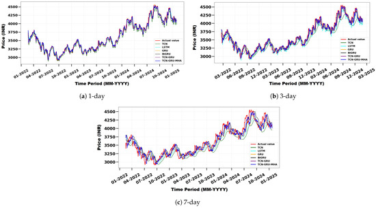
Figure 8. Comparison of actual and predicted TCS stock prices using TCN, LSTM, GRU, BiGRU, TCN-GRU, and the proposed model for different forecast horizons: (a) 1 day, (b) 3 days, and (c) 7 days.

4.3. Performance Evaluation on TSLA Stock Data

This part includes a detailed analysis of the predictability of the prices of TSLA stocks in the time series. The forecasting capability of the proposed model is analyzed over three different prediction horizons, namely, 1 day, 3 days, and 7 days. The results are summarized in Table 7. Strong values of ${\mathrm{R}}^2$ and low RMSE for each forecast horizon suggest that the model is reliable and accurate in capturing the complex dynamics of TSLA stock prices. The forecast for 1 day achieves an RMSE of 0.049 and an ${\mathrm{R}}^2$ of 0.978. This highlights the excellent accuracy of short-term predictions. On the three-day horizon, the model achieves consistency, an RMSE of 0.083, and an ${\mathrm{R}}^2$ of 0.944. Even in the 7-day prediction, where accuracy tends to decay, the model outperforms every benchmark. The model achieves an RMSE of 0.141 and ${\mathrm{R}}^2$ of 0.839. These results validate the robustness of the framework and are indicative of its functionality for short-term stock predictions.

Table 7. Summary of model performance in predicting TSLA stock prices over 1-day, 3-day, and 7-day time frames.

Time Frame	Model	RMSE	MAE	MAPE	R2
1 Day	TCN	$0.082$	$0.055$	$4.42\%$	$0.932$
	LSTM	$0.071$	$0.050$	$4.12\%$	$0.940$
	GRU	$0.062$	$0.044$	$3.82\%$	$0.957$
	BiGRU	$0.058$	$0.042$	$2.55\%$	$0.961$
	TCN-GRU	$0.053$	$0.038$	$2.44\%$	$0.972$
	Proposed Model	$0.049$	$0.036$	$2.37\%$	$0.978$
3 Days	TCN	$0.120$	$0.085$	$6.13\%$	$0.880$
	LSTM	$0.113$	$0.081$	$6.02\%$	$0.893$
	GRU	$0.101$	$0.074$	$5.78\%$	$0.917$
	BiGRU	$0.097$	$0.072$	$4.70\%$	$0.923$
	TCN-GRU	$0.089$	$0.068$	$4.58\%$	$0.937$
	Proposed Model	$0.083$	$0.065$	$4.45\%$	$0.944$
7 Days	TCN	$0.188$	$0.132$	$9.03\%$	$0.763$
	LSTM	$0.175$	$0.124$	$8.80\%$	$0.782$
	GRU	$0.163$	$0.118$	$7.62\%$	$0.800$
	BiGRU	$0.162$	$0.115$	$7.53\%$	$0.808$
	TCN-GRU	$0.150$	$0.110$	$7.37\%$	$0.825$
	Proposed Model	$0.141$	$0.107$	$7.22\%$	$0.839$

Figure 9 compares actual and predicted TSLA stock prices using TCN, LSTM, GRU, BiGRU, TCN-GRU, and the proposed TCN-GRU-MHA model across different forecast horizons: (a) 1-day, (b) 3-day, and (c) 7-day. The x-axis represents the timeline (month–year), and the y-axis represents the stock price in (USD).The model is superior to the baseline methods and is very similar to the real values. It effectively identifies short-term trends through the use of multi-head attention, highlighting its versatility and effectiveness in forecasting stock prices.

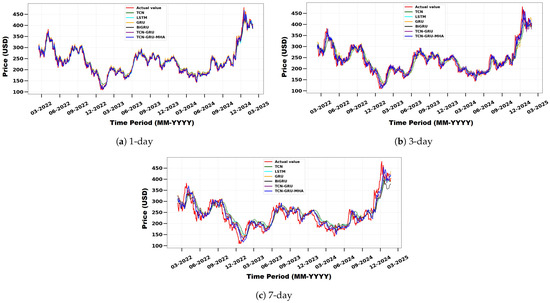
Figure 9. Comparison of actual and predicted TSLA stock prices using TCN, LSTM, GRU, BiGRU, TCN-GRU, and the proposed model for different forecast horizons: (a) 1 day, (b) 3 days, and (c) 7 days.

4.4. Performance Evaluation on Nifty 50 Index Dataset

We compare TCN-GRU-MHA with the baseline models TCN, LSTM, GRU, BiGRU, and TCN-GRU on varying prediction horizons: 1 day, 3 days, and 7 days. Table 8 shows the comparison results based on the measures RMSE, MAE, MAPE, and ${\mathrm{R}}^2$. This offers an overall comparison of the models based on predictability. This provides a comprehensive comparison of predictive accuracy and error reduction models. For the 1-day forecast, the proposed model performs the best, with an RMSE of 0.132 and an ${\mathrm{R}}^2$ score of 0.983. These results show that the model is highly accurate in capturing short-term changes. The next best model, TCN-GRU, shows slightly higher errors and a lower ${\mathrm{R}}^2$ of $0.980$. The 3-day forecast shows that the proposed model gives the best results, with an RMSE of 0.234 and an ${\mathrm{R}}^2$ of 0.942. This means that the model remains accurate for an extended period of time. Although prediction uncertainty increases for the 7-day forecast, the proposed model still leads, with an RMSE of $0.403$ and ${\mathrm{R}}^2$ of $0.840$. Despite a slight performance drop, it outperforms TCN-GRU ($0.836$) and GRU ($0.830$) and significantly outperforms TCN ($0.794$), confirming its robustness across varying forecast horizons.

Table 8. Summary of model performance in predicting NIFTY 50 index prices over 1-day, 3-day, and 7-day time frames.

Time Frame	Model	RMSE	MAE	MAPE	R2
1 Day	TCN	$0.236$	$0.190$	$4.47\%$	$0.930$
	LSTM	$0.207$	$0.167$	$3.73\%$	$0.945$
	GRU	$0.173$	$0.140$	$2.83\%$	$0.963$
	BiGRU	$0.156$	$0.128$	$2.43\%$	$0.971$
	TCN-GRU	$0.138$	$0.115$	$1.98\%$	$0.980$
	Proposed Model	$0.132$	$0.110$	$1.84\%$	$0.983$
3 Days	TCN	$0.350$	$0.281$	$6.85\%$	$0.882$
	LSTM	$0.328$	$0.259$	$6.31\%$	$0.893$
	GRU	$0.301$	$0.237$	$5.63\%$	$0.907$
	BiGRU	$0.276$	$0.218$	$4.98\%$	$0.920$
	TCN-GRU	$0.246$	$0.194$	$4.21\%$	$0.936$
	Proposed Model	$0.234$	$0.185$	$3.91\%$	$0.942$
7 Days	TCN	$0.503$	$0.413$	$9.46\%$	$0.794$
	LSTM	$0.479$	$0.390$	$8.91\%$	$0.805$
	GRU	$0.451$	$0.369$	$8.24\%$	$0.818$
	BiGRU	$0.425$	$0.342$	$7.65\%$	$0.830$
	TCN-GRU	$0.412$	$0.331$	$7.33\%$	$0.836$
	Proposed Model	$0.403$	$0.324$	$7.12\%$	$0.840$

Figure 10 illustrates the predicted versus actual stock prices for the Nifty 50 index. The comparison highlights the effectiveness of the proposed model in consistently delivering more accurate predictions across all time frames. Even with the increased uncertainty of the 7-day forecast, the model continues to deliver relatively accurate predictions compared with the baseline models. These visual results show that the model is strong and can predict short-term stock prices.

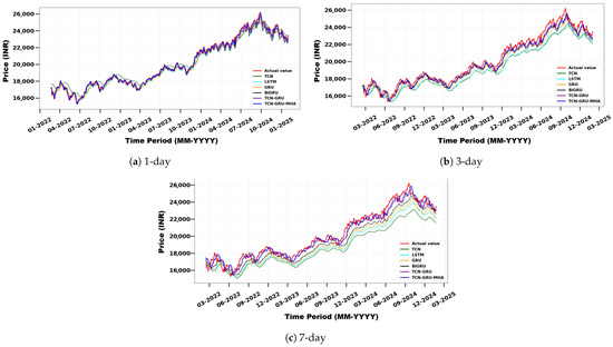
Figure 10. Comparison of actual and predicted Nifty 50 index prices using TCN, LSTM, GRU, BiGRU, TCN-GRU, and the proposed model for different forecast horizons: (a) 1 day, (b) 3 days, and (c) 7 days.

4.5. Performance Evaluation on S&P 500 Index Dataset

To ensure a thorough assessment of the proposed deep learning model, we executed experiments on a diverse range of assets. The Nifty 50 index represents the performance of the largest large-cap companies in India, while the S&P 500 index tracks 500 of the largest publicly traded companies in the United States, serving as a global benchmark for equity market trends. Incorporating both indices alongside individual stocks allows the model’s performance to be tested across different market structures, economic environments, and volatility patterns.

Table 9 shows the results for the S&P 500 dataset at 1-day, 3-day, and 7-day prediction intervals. The baseline models (TCN, LSTM, GRU, BiGRU, and TCN-GRU) always perform better than the proposed model. Across all periods, these baseline models had higher ${\mathrm{R}}^2$ values and lower prediction errors. For the 1-day forecast, the proposed model performs the best, with an RMSE of 0.155 and an ${\mathrm{R}}^2$ score of 0.979. The next best model, TCN-GRU, shows slightly higher errors and a lower ${\mathrm{R}}^2$ of 0.975. The 3-day forecast shows that the proposed model gives the best results, with an RMSE of 0.251 and an ${\mathrm{R}}^2$ of 0.940. This means that the model remains accurate for an extended period of time. Although the uncertainty of the prediction increases for the 7-day forecast, the proposed model still leads, with an RMSE of 0.438 and ${\mathrm{R}}^2$ of 0.837.

Table 9. Summary of model performance in predicting S&P 500 index prices over 1-day, 3-day, and 7-day time frames.

Time Frame	Model	RMSE	MAE	MAPE	R2
1 Day	TCN	$0.275$	$0.196$	$4.60\%$	$0.928$
	LSTM	$0.242$	$0.169$	$3.85\%$	$0.942$
	GRU	$0.197$	$0.131$	$2.98\%$	$0.962$
	BiGRU	$0.182$	$0.118$	$2.61\%$	$0.968$
	TCN-GRU	$0.165$	$0.104$	$2.20\%$	$0.975$
	Proposed Model	$0.155$	$0.096$	$1.98\%$	$0.979$
3 Days	TCN	$0.365$	$0.271$	$6.38\%$	$0.892$
	LSTM	$0.336$	$0.247$	$5.74\%$	$0.904$
	GRU	$0.314$	$0.231$	$5.32\%$	$0.913$
	BiGRU	$0.281$	$0.202$	$4.61\%$	$0.927$
	TCN-GRU	$0.260$	$0.183$	$4.18\%$	$0.936$
	Proposed Model	$0.251$	$0.175$	$3.97\%$	$0.940$
7 Days	TCN	$0.557$	$0.460$	$9.96\%$	$0.788$
	LSTM	$0.526$	$0.435$	$9.43\%$	$0.801$
	GRU	$0.486$	$0.404$	$8.71\%$	$0.816$
	BiGRU	$0.467$	$0.387$	$8.30\%$	$0.824$
	TCN-GRU	$0.452$	$0.373$	$7.94\%$	$0.831$
	Proposed Model	$0.438$	$0.360$	$7.65\%$	$0.837$

Figure 11 compares actual and predicted S&P 500 prices across three forecast horizons: (a) 1 day, (b) 3 days, and (c) 7 days, using baseline models and the proposed TCN-GRU-MHA. The x-axis represents the timeline formatted as month-year, while the y-axis represents the index price in dollars (USD). The model outperforms traditional methods and stays close to real values. It captures short-term trends well using multi-head attention. This shows its flexibility and effectiveness in stock price forecasting.

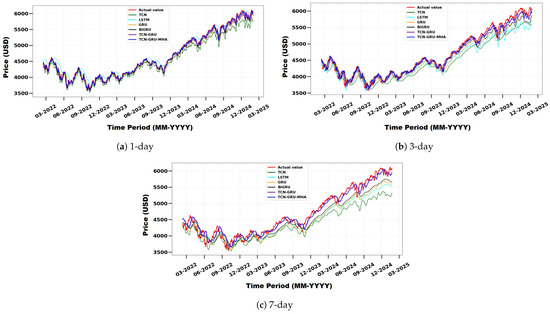
Figure 11. Comparison of actual and predicted S&P500 stock prices using TCN, LSTM, GRU, BiGRU, TCN-GRU, and the proposed model for different forecast horizons: (a) 1 day, (b) 3 days, and (c) 7 days.

4.6. Comparative Evaluation of Baseline and Proposed Models

We compare the proposed TCN–GRU–MHA model with two standard statistical baselines: the ARIMA (autoRegressive integrated moving average) model and the Random Walk Model (also referred to as the Naïve last-price model). ARIMA is a classical time-series technique that models linear relationships in historical data. It uses autoregression to capture past values, differencing to remove trends, and moving averages to account for previous forecast errors. In contrast, the Random Walk Model predicts that the closing price for the next day will be the same as the closing price for the previous day, serving as a simple yet strong reference baseline.

We evaluated all baseline models and compared their performance with the proposed model over a 1-day time frame. The evaluation was carried out on all five datasets used in this study. RMSE and MAE are presented on a normalized scale, while MAPE and ${\mathrm{R}}^2$ are reported on the actual scale to enhance clarity and interpretability. The results indicate that ARIMA consistently underperforms compared with the Random Walk Model, which offers superior forecast accuracy despite its simplicity. The proposed hybrid deep learning model outperforms both baselines on all datasets, demonstrating its strength and superior capability in stock price prediction. Table 10 presents a detailed comparison of the prediction results obtained from ARIMA, the Random Walk Model, and the proposed hybrid approach.

Table 10. Performance comparison of baseline and proposed models for 1-day-ahead predictions across multiple datasets.

Dataset	Model	RMSE	MAE	MAPE	${\mathbf{R}}^2$
HDFC Bank	ARIMA	0.245	0.196	11.28%	0.310
	Random Walk Model	0.046	0.027	3.83%	0.932
	Proposed Model	0.014	0.008	1.21%	0.981
TCS	ARIMA	0.411	0.321	8.64%	0.356
	Random Walk Model	0.094	0.065	2.03%	0.915
	Proposed Model	0.072	0.050	1.44%	0.987
TSLA	ARIMA	0.362	0.287	11.83%	0.137
	Random Walk Model	0.085	0.063	4.24%	0.890
	Proposed Model	0.049	0.036	2.37%	0.978
Nifty 50	ARIMA	0.428	0.341	7.52%	0.216
	Random Walk Model	0.172	0.142	2.39%	0.920
	Proposed Model	0.132	0.110	1.84%	0.983
S&P 500	ARIMA	0.335	0.246	10.24%	0.292
	Random Walk Model	0.205	0.155	3.18%	0.906
	Proposed Model	0.155	0.096	1.98%	0.979

The results of the sblation study, conducted to quantify the incremental contributions of TCN, GRU, MHA, and the feature selection step, for all five datasets across the 1-day, 3-day, and 7-day forecast horizons are provided in the Supplementary Material (Tables S1–S5). Additionally, error-bar analyses corresponding to the existing models and the proposed model for the same datasets and horizons are presented separately in the Supplementary Material (Figures S1–S5).

4.7. Comparison of Predictive Performance with Other Approaches

To further contextualize the effectiveness of the proposed model, TCN-GRU-MHA, we compared its performance with several recent deep learning models that performed a stock price prediction using regression on the same dataset utilized in this study. Table 11 presents the prediction accuracy of these models, focusing on the ${\mathrm{R}}^2$ score and RMSE for the 1-day horizon reported in the literature.

Table 11. Comparison of the proposed model with other models on the 1-day time frame, with emphasis on the ${\mathrm{R}}^2$ score and RMSE.

Reference	Technique Used	Dataset	${\mathbf{R}}^2$	RMSE
Fathali et al. (2022)	LSTM (H-L-O-C feature)	Nifty 50	$0.537$	0.082
Fozap (2025)	LSTM-CNN	S&P 500	$0.419$	0.101
Fozap (2025)	Random Forest	S&P 500	$0.565$	0.085
Sarıkoç and Celik (2024)	PCA-ICA-LSTM	S&P 500	$0.951$	–
Li et al. (2024)	TCN-GRU	S&P 500	$0.940$	68.896
Li et al. (2024)	TCN-GRU-CBAM	S&P 500	$0.965$	52.187
Proposed model	TCN-GRU-MHA	Nifth 50	$0.983$	0.132
Proposed model	TCN-GRU-MHA	S&P 500	$0.979$	0.155

4.8. Statistical Tests for Model Evaluation and Data Stationarity

We conducted two statistical tests to ensure the reliability of our results and the appropriateness of the data for forecasting. The first one was the Friedman test, a nonparametric statistical method used to compare three or more related groups, particularly when the assumption of normality is violated. In this study, the Friedman test was used to assess whether the observed performance differences between prediction models were statistically significant. The second test was the Augmented Dickey–Fuller (ADF) test, a widely used statistical method to detect the presence of a unit root in a time series and determine its stationarity. The null hypothesis assumes that the series is non-stationary, while the alternative hypothesis indicates stationarity.

The Friedman test was applied to the RMSE scores of six models evaluated over three forecast horizons (1 day, 3 days, and 7 days) for three major stocks, HDFC Bank, TCS, and TSLA, as well as two indices, Nifty 50 and S&P 500. The test yielded an identical statistic of $14.619$ for HDFC Bank and TCS, with a p-value of $0.0121$. For the TSLA stock, the test produced a statistic of $15.0$ and a p-value of $0.0103$. The Nifty 50 and S&P 500 Index produced the same statistic value of $15.0$ and a p-value of $0.0103$. These results show that there are statistically significant differences in model performance among the forecast horizons (p < $0.05$). This shows how forecast length affects predictive accuracy and further indicates the strength of the proposed model.

To evaluate the stationarity of the data, the ADF test was conducted on the closing price series of the entire dataset. The results yielded high p-values (all > $0.05$) and test statistics exceeding the critical values at the 1% ($-3.4330$), 5% ($-2.8627$), and 10% ($-2.5674$) significance levels. This indicates that all price series are non-stationary, necessitating transformation or differencing prior to further modeling. Table 12 summarizes the findings of the ADF test.

Table 12. Summary of ADF test results for the closing prices of selected stocks and indices.

Stock/Index Name	Test Statistic	p-Value
HDFC Bank	−1.061	0.730
TCS	−0.472	0.897
HUL	−0.596	0.871
Nifty 50	0.366	0.980
S&P 500	0.612	0.987

5. Conclusions

This study proposes a new hybrid deep learning framework, TCN-GRU-MHA, designed to improve the accuracy of short-term stock price prediction on the 1-day, 3-day, and 7-day horizons. The model combines the strengths of TCNs for time-domain feature extraction, GRUs for learning sequence patterns, and MHA to dynamically highlight the most important information from stock time-series data. Furthermore, the hybrid feature selection method—combining an improved RFE technique, model-based importance scores (from random forest and gradient boosting), and Kendall tau correlation—helps identify the most relevant features using a 75:25 weighted scheme. Experimental tests were conducted on three major stocks, HDFC Bank, TCS, and TSLA, as well as two indices: Nifty 50 and S&P 500. The results showed that the proposed model consistently outperformed several other models, including TCN, LSTM, GRU, BiGRU, and TCN-GRU. The evaluation was performed using standard metrics, i.e., RMSE, MAE, MAPE and ${\mathrm{R}}^2$, where the hybrid model delivered better results on all benchmarks.

Future research could explore various fascinating possibilities. Integrating additional data sources such as financial news, macroeconomic indicators, and sentiment on social media can help better understand how the market works and make more accurate predictions. From the perspective of methodology, alternative attention mechanisms (such as hierarchical attention, cross-attention, or self-attention) and ensemble learning techniques that integrate deep learning variants can be explored to improve their robustness. New architectures such as Transformer variants and advanced hyperparameter optimization methods such as Bayesian optimization may make the model much better at capturing long-term dependencies.

References

- Atesongun, A., & Gulsen, M. (2024). A hybrid forecasting structure based on ARIMA and artificial neural network models. Applied Sciences, 14(16), 7122. [Google Scholar] [CrossRef]
- Caiado, J., & Lúcio, F. (2023). Stock market forecasting accuracy of asymmetric GARCH models during the COVID-19 pandemic. The North American Journal of Economics and Finance, 68, 101971. [Google Scholar] [CrossRef]
- Chen, C., Xue, L., & Xing, W. (2023). Research on improved GRU-based stock price prediction method. Applied Sciences, 13(15), 8813. [Google Scholar] [CrossRef]
- Chi, D.-J., & Chu, C.-C. (2021). Artificial intelligence in corporate sustainability: Using LSTM and GRU for going concern prediction. Sustainability, 13(21), 11631. [Google Scholar] [CrossRef]
- Chinta, S. (2021). Integrating machine learning algorithms in big data analytics: A framework for enhancing predictive insights. IJARESM, 9, 2145–2161. [Google Scholar] [CrossRef]
- Chopra, R., & Sharma, G. D. (2021). Application of artificial intelligence in stock market forecasting: A critique, review, and research agenda. Journal of Risk and Financial Management, 14(11), 526. [Google Scholar] [CrossRef]
- Fathali, Z., Kodia, Z., & Ben Said, L. (2022). Stock market prediction of Nifty 50 index applying machine learning techniques. Applied Artificial Intelligence, 36(1), 2111134. [Google Scholar] [CrossRef]
- Fozap, F. M. P. (2025). Hybrid machine learning models for long-term stock market forecasting: Integrating technical indicators. Journal of Risk and Financial Management, 18(4), 201. [Google Scholar] [CrossRef]
- Friday, I. K., Pati, S. P., Mishra, D., Mallick, P. K., & Kumar, S. (2024). CAGTRADE: Predicting stock market price movement with a CNN-Attention-GRU model. Asia-Pacific Financial Markets, 32, 583–608. [Google Scholar] [CrossRef]
- Gautam, B., Kandel, S., Shrestha, M., & Thakur, S. (2024). Comparative analysis of machine learning models for stock price prediction: Leveraging LSTM for real-time forecasting. Journal of Computer and Communications, 12(8), 52–80. [Google Scholar] [CrossRef]
- Guo, C., Kang, X., Xiong, J., & Wu, J. (2023). A new time series forecasting model based on complete ensemble empirical mode decomposition with adaptive noise and temporal convolutional network. Neural Processing Letters, 55(4), 4397–4417. [Google Scholar] [CrossRef]
- Hoseinzade, E., & Haratizadeh, S. (2019). CNNpred: CNN-based stock market prediction using a diverse set of variables. Expert Systems with Applications, 129, 273–285. [Google Scholar] [CrossRef]
- Jaiswal, R., & Singh, B. (2022, April 23–24). A hybrid convolutional recurrent (CNN-GRU) model for stock price prediction. 2022 IEEE 11th International Conference on Communication Systems and Network Technologies (CSNT) (pp. 299–304), Indore, India. [Google Scholar] [CrossRef]
- Kanwal, A., Lau, M. F., Ng, S. P., Sim, K. Y., & Chandrasekaran, S. (2022). BiCuDNNLSTM-1dCNN—A hybrid deep learning-based predictive model for stock price prediction. Expert Systems with Applications, 202, 117123. [Google Scholar] [CrossRef]
- Kervanci, I. S., Akay, M. F., & Özceylan, E. (2024). Bitcoin price prediction using LSTM, GRU and hybrid LSTM-GRU with bayesian optimization, random search, and grid search for the next days. Journal of Industrial and Management Optimization, 20(2), 570–588. [Google Scholar] [CrossRef]
- Khodaee, P., Esfahanipour, A., & Taheri, H. M. (2022). Forecasting turning points in stock price by applying a novel hybrid CNN-LSTM-ResNet model fed by 2D segmented images. Engineering Applications of Artificial Intelligence, 116, 105464. [Google Scholar] [CrossRef]
- Kurani, A., Doshi, P., Vakharia, A., & Shah, M. (2023). A comprehensive comparative study of artificial neural network (ANN) and support vector machines (SVM) on stock forecasting. Annals of Data Science, 10(1), 183–208. [Google Scholar] [CrossRef]
- Lei, K., Zhang, B., Li, Y., Yang, M., & Shen, Y. (2020). Time-driven feature-aware jointly deep reinforcement learning for financial signal representation and algorithmic trading. Expert Systems with Applications, 140, 112872. [Google Scholar] [CrossRef]
- Li, S., Huang, X., Cheng, Z., Zou, W., & Yi, Y. (2023). AE-ACG: A novel deep learning-based method for stock price movement prediction. Finance Research Letters, 58, 104304. [Google Scholar] [CrossRef]
- Li, S., Tang, G., Chen, X., & Lin, T. (2024). Stock index forecasting using a novel integrated model based on CEEMDAN and TCN-GRU-CBAM. IEEE Access, 12, 122524–122543. [Google Scholar] [CrossRef]
- Luo, A., Zhong, L., Wang, J., Wang, Y., Li, S., & Tai, W. (2024). Short-term stock correlation forecasting based on CNN-BiLSTM enhanced by attention mechanism. IEEE Access, 12, 29617–29632. [Google Scholar] [CrossRef]
- Mostafavi, S. M., & Hooman, A. R. (2025). Key technical indicators for stock market prediction. Machine Learning with Applications, 20, 100631. [Google Scholar] [CrossRef]
- Naeem, M., Jassim, H. S., & Korsah, D. (2024). The application of machine learning techniques to predict stock market crises in Africa. Journal of Risk and Financial Management, 17(12), 554. [Google Scholar] [CrossRef]
- Nourbakhsh, Z., & Habibi, N. (2023). Combining LSTM and CNN methods and fundamental analysis for stock price trend prediction. Multimedia Tools and Applications, 82(12), 17769–17799. [Google Scholar] [CrossRef]
- Parray, I. R., Khurana, S. S., Kumar, M., & Altalbe, A. A. (2020). Time series data analysis of stock price movement using machine learning techniques. Soft Computing-A Fusion of Foundations, Methodologies & Applications, 24(21), 16509–16517. [Google Scholar] [CrossRef]
- Priyatno, A. M., & Widiyaningtyas, T. (2024). A systematic literature review: Recursive feature elimination algorithms. JITK (Jurnal Ilmu Pengetahuan dan Teknologi Komputer), 9(2), 196–207. [Google Scholar] [CrossRef]
- Salem, F. M. (2021). Gated RNN: The gated recurrent unit (GRU) RNN. In Recurrent neural networks: From simple to gated architectures (pp. 85–100). Springer. [Google Scholar] [CrossRef]
- Sarıkoç, M., & Celik, M. (2024). PCA-ICA-LSTM: A hybrid deep learning model based on dimension reduction methods to predict S&P 500 index price. Computational Economics, 65, 2249–2315. [Google Scholar] [CrossRef]
- Selvamuthu, D., Kumar, V., & Mishra, A. (2019). Indian stock market prediction using artificial neural networks on tick data. Financial Innovation, 5(1), 16. [Google Scholar] [CrossRef]
- Sirisha, U. M., Belavagi, M. C., & Attigeri, G. (2022). Profit prediction using ARIMA, SARIMA and LSTM models in time series forecasting: A comparison. IEEE Access, 10, 124715–124727. [Google Scholar] [CrossRef]
- Teixeira, D. M., & Barbosa, R. S. (2024). Stock price prediction in the financial market using machine learning models. Computation, 13(1), 3. [Google Scholar] [CrossRef]
- Wang, Z., & Peng, Z. (2024). Structural acceleration response reconstruction based on BiLSTM network and multi-head attention mechanism. Structures, 64, 106602. [Google Scholar] [CrossRef]
- Wen, X., Liao, J., Niu, Q., Shen, N., & Bao, Y. (2024). Deep learning-driven hybrid model for short-term load forecasting and smart grid information management. Scientific Reports, 14(1), 13720. [Google Scholar] [CrossRef] [PubMed]
- Xiaoyan, H., Bingjie, L., Jing, S., Hua, L., & Guojing, L. (2021, September 27–29). A novel forecasting method for short-term load based on TCN-GRU model. 2021 IEEE International Conference on Energy Internet (ICEI) (pp. 79–83), Southampton, UK. [Google Scholar] [CrossRef]
- Yang, S., Guo, H., & Li, J. (2022). CNN-GRUA-FC stock price forecast model based on multi-factor analysis. Journal of Advanced Computational Intelligence and Intelligent Informatics, 26(4), 600–608. [Google Scholar] [CrossRef]
- Zhou, S., Song, C., Wang, T., Pan, X., Chang, W., & Yang, L. (2022). A short-term hybrid TCN-GRU prediction model of bike-sharing demand based on travel characteristics mining. Entropy, 24(9), 1193. [Google Scholar] [CrossRef] [PubMed]
Disclaimer/Publisher’s Note: The statements, opinions and data contained in all publications are solely those of the individual author(s) and contributor(s) and not of MDPI and/or the editor(s). MDPI and/or the editor(s) disclaim responsibility for any injury to people or property resulting from any ideas, methods, instructions or products referred to in the content. |
© 2025 by the authors. Licensee MDPI, Basel, Switzerland. This article is an open access article distributed under the terms and conditions of the Creative Commons Attribution (CC BY) license (https://creativecommons.org/licenses/by/4.0/).