A Model-Free Lattice

Abstract

Predicting future price movements has always been one of the major topics in financial research, and there is no better method to predict the future prices of an asset than using its derivatives. In this paper, we propose a model-free lattice model that describes the complete price evolution of the underlying asset and simultaneously re-prices all of its European options. Given that such a lattice is consistent with market option prices, it must embed all necessary risk factors (e.g., random volatility, random interest rates, and jumps) and market restrictions (e.g., mean-reversion and liquidity) that are priced into the European options.

1. Introduction

Predicting future price movements has always been one of the major topics in financial research, and there is no better method to predict the future prices of an asset than using its derivatives (e.g., option). This is because derivative prices embed projections of the underlying asset (as they are various bets on the future performance of the underlying asset), and they reflect a market view of the future price distribution of the underlying asset. If the derivative contract is on a broad market index (such as an S&P index, an interest rate, or a foreign exchange), then its projection is critically important for market participants and even regulators.

In the literature, using derivative prices to back out information about their underlying asset has a long history, beginning with Banz and Miller (1978) and Breeden and Litzenberger (1978). They contend that if one takes a partial derivative of an option price with respect to its strike price, then one obtains the risk-neutral probability of the option being in the money at the maturity date (after being discounted at the risk-free rate). If there were a continuous spectrum of option prices, then one could derive the entire (risk-neutral) probability distribution of the underlying asset at the maturity date. With multiple maturity dates, one can project the evolution of the probability distributions of the underlying asset over time.

There are, broadly speaking, two approaches to exploring Banz and Miller (1978) and Breeden and Litzenberger (1978). One approach is to estimate a the pricing kernel (also known as state price density) using derivative prices, which is pioneered by Aït-Sahalia and Lo (1998),1 who derive a non-parametric-state price density using S&P 500 index options (daily data of whole year of 1993).2 To improve the tractability, they apply smoothing and dimension reduction to their pricing kernel. Hence, even though smoothing and dimension reduction do not rely on any distributional assumptions, their pricing kernel is not entirely non-parametric (strictly speaking) in that there are still parameters (e.g., bandwidth) in these techniques that remain to be estimated or arbitrarily specified. An undesirable side effect of smoothing and dimension reduction is that options are then not completely re-priced. While the literature on pricing kernels is voluminous, it is unrelated to our paper. Interested readers can see Cuesdeanu and Jackwerth (2018) for an excellent review.

Our work is related to the other approach, which is to develop a lattice that is consistent with the market derivative prices. The first such effort is the implied binomial model by Rubinstein (1994), among others.3 As we are well aware, traditional lattice models (pioneered by, among others, the binomial model of Cox et al. (1979)) are based upon parametric models such as the Black–Scholes (log-normal, 1973) or the Cox (square root, Cox, 1975) model.4 These parametric models are highly limited and mis-price badly, even European options (let alone more complex derivatives). To remedy this shortcoming, option-implied lattices have been developed. While Rubinstein (1994) tweaks the binomial model to fit existing option prices, a similar and yet different approach that tries to discretize a flexible process (known as the local volatility model) is discovered by Dupire (1994) and Derman and Kani (1994).

Although both of the above approaches (pricing kernel and implied lattice) claim that they can successfully use option prices to recover the entire risk-neutral density of the underlying asset, they suffer from one common shortcoming—they only can recover one density function of a given time in the future. There is no description of how the asset price evolves over time. Britten-Jones and Neuberger (2000) fill this gap by providing a flexible stochastic process for the underlying asset.

Britten-Jones and Neuberger (2000) claim that the stochastic process they derive is consistent with most processes that accommodate stochastic volatility. Their model can be viewed (as themselves admit) as an extension to Dupire (1994) and Derman and Kani (1994) in that their model allows for random volatility, whereas the models by Dupire (1994) and Derman and Kani (1994) do not. Although they claim that their model can re-price most options (their Proposition 1), unfortunately, a restriction in their model (their Equation (18)) fails to support their claim.

Our contribution to the literature is to extend Britten-Jones and Neuberger (2000) in the following two directions. Firstly, our lattice can be viewed as a direct extension of the Britten-Jones–Neuberger model, just like the Cox–Ross–Rubinstein lattice being an extension to the Black–Scholes model. Such an extension allows complex options (e.g., American options) to be consistently evaluated. In practice, an option pricing model is calibrated to liquid simple options (e.g., swaptions), and then, the corresponding lattice is used to price complex options (e.g., range accruals).

Secondly, our model is more flexible than the Britten-Jones–Neuberger model in that our lattice can accurately re-price all European options across different strikes and over different maturities. In other words, one can view our lattice as a model that allows for all random factors that affect market option prices (such factors could be other interest rate factors such as random interest rates and jumps, as well as market conditions such as liquidity).

Finally, to derive a continuous-time stochastic process from our lattice, so that we can visualize the evolution of the underlying asset as in Dupire (1994), Derman and Kani (1994), and Britten-Jones and Neuberger (2000), we adopt the technology of a copula. As is widely known, a copula specifies a joint distribution with any given number of marginal distributions. As various risk-neutral densities are identified via traded European options (each risk-neutral density function corresponds to a maturity), the use of a copula can “string” them into a stochastic process. As a result, our lattice can be viewed as a well-specified stochastic process for the underlying asset.

For the remainder of the paper, we first describe a discrete risk-neutral density so that all options can be exactly re-priced. Then we review how a flexible lattice can be constructed. The section of model-free lattice is the main contribution of this paper. Finally an example is given, and then, the paper concludes.

2. The Risk-Neutral Density (RND)

Given that derivative prices are bets (by market participants) on future prices of the underlying asset, they are useful in retrieving the market perception of the future behaviors of the underlying asset.

Option-implied risk-neutral density, pioneered by Banz and Miller (1978) and Breeden and Litzenberger (1978), prove that the risk-neutral probability distribution function (i.e., cumulative density function) can be derived as follows:

$$F(K)={\displaystyle \frac{\partial C}{\partial K}}=\mathrm{Pr}[S>K]$$

(1)

Taking another derivative, we obtain the risk-neutral density (RND) function:5

$$f(K)={\displaystyle \frac{\partial F(K)}{\partial K}}={\displaystyle \frac{{\partial }^{2}C}{\partial K^2}}$$

(2)

Among others, show that in the case of a continuum collection of European option prices (across both maturities and strikes), they can completely span the asset state space. As a result, these European options can duplicate any exotic options on the same underlying asset. Plainly speaking, with a continuum collection (i.e., infinite number) of option prices, we can then identify a joint probability distribution over time based on the option prices without a model (i.e., model-free).

However, in reality, the number of option contracts traded in the market is limited. In fact, many stocks have very few options traded in the market. As a result, some parametric structure (i.e., a functional form) of the density function must be assumed. Hence, determining how to retrieve risk-neutral density (RND) functions from option prices is a challenging exercise and has attracted a lot of attention. This is because, given a finite number of options traded in the marketplace, the RND function is not uniquely defined. Various methods are proposed to remedy the lack of enough option prices. The literature has used four different methods:

• Smoothing in the volatility space;
• Smoothing in the price space;
• Smoothing in the density space.

Volatility smoothing has been the most popular method used in identifying the RND. Under this approach, due to the forced smoothness of the fitted volatility function, not all options can be exactly re-priced. Nevertheless, by enforcing a smooth function through the volatilities, a number of “fake options” are created in order to fulfill Equation (1). In contrast, few researchers use price smoothing. Interested readers can find excellent references in Orosi (2015). Finally, various attempts have been made to find the best functional form for the density function. Lai (2014) provides an excellent review of the existing methods.6

While seeking a methodology that can best retrieve information from option prices is an interesting research topic on its own right, it is not the main focus of our paper. Unlike the literature, in this paper, we do not allow for pricing errors in the discrete setting (and yet, at the same time, guarantee convergence in continuous time).

In this paper, we use the piece-wise flat RND to calibrate to the option prices such that the repricing of options is guaranteed (no pricing errors). The piece-wise flat RND exactly matches the options traded in the marketplace. There are two advantages of using the piece-wise flat RND. First, empirically, when compared to more complicated methods, such RNDs are very stable over time. Second, the RND has a closed-form solution which is easy and fast to solve. Third, the number of options can vary from one maturity to another (a term structure of RNDs), and yet, through construction, all options are priced perfectly, and as a result, the number is uniquely defined (same degrees of freedom as the number of options).

As it turns out, the piece-wise flat RNDs maintain the most information from option prices. Other higher-power polynomials (we also use piece-wise linear and cubic-spline as a robust check) over-fit the density and result in losing useful information.

The piece-wise flat density function is demonstrated in Figure 1. Figure 1 provides a simple demonstration of a three-option example. In Figure 1, three call options are given and a risk-neutral density is provided so that the values calculated by Equations (3)–(6) can perfectly match the market values of these options.

This density function can exactly re-price all options for that maturity.

$$\begin{array}{ll}{C}_k& ={\displaystyle {\int }_{K_k}^x}(S-K_k)\varphi (S)dS\\ & ={\displaystyle \frac{1}{2}}{\displaystyle {\sum }_{i=k}^n}{a}_i(K_{i+1}^2-K_i^2)-K_k{\displaystyle {\sum }_{i=k}^n}{a}_i(K_{i+1}-K_i)\end{array}$$

(3)

where $K_0=0$, and the density function’s right-most value is

$$x=K_n+{\displaystyle \frac{1}{a_n}}\left[1-{\displaystyle {\sum }_{i=1}^n}{a}_{i-1}(K_i-K_{i-1})\right]$$

(4)

Then, we can solve for the densities, $a_k$ (where $k=0,\cdots ,n$), in closed form:

$$a_n={\displaystyle \frac{2C_n}{{(x-K_n)}^2}}$$

(5)

and

$$a_k={\displaystyle \frac{2}{{(K_{k+1}-K_k)}^2}}\left[C_k-{\displaystyle \frac{1}{2}}{\displaystyle {\sum }_{i=k+1}^n}{a}_i\left[(K_{i+1}^2-K_i^2)-2K_k(K_{i+1}-K_i)\right]\right]$$

(6)

with $C_0=S_0$ and $K_0=0$. By iterating $x$, we can solve for all the $a$ s.

Our major objective is to connect the multiple RNDs implied by the options of various maturity dates. In other words, we wish to derive an “implied stochastic process” for the underlying asset that is consistent with the traded option prices with all strikes at all maturities. Unfortunately, there is no unique way to construct such a stochastic process. In this paper, we use a copula to connect two consecutive RNDs.

3. The Lattice

Imagine a trinomial lattice as a discrete approximation of a stochastic process in continuous time (i.e., mimicking continuous time with a very small $\Delta t$). An example is given in Figure 2.

This forward-expanding trinomial lattice is equivalent to the explicit finite difference method (see Hull (2015)), which is a discretized backward partial differential equation (PDE) in continuous time that a derivative price must satisfy. One can implement a backward-expanding lattice, which is equivalent to the implicit finite difference method (see Hull (2015)). The implicit finite difference method is a discretized forward partial differential equation (PDE). Both lattices will converge to the continuous time limit efficiently. As a result, we regard this trinomial lattice as the (approximated) continuous time process.

In the most general case (shown in the lower-left corner of Figure 2), the probabilities of the branches can be both state-dependent and time-dependent. In other words, this trinomial lattice can be made consistent with any given stochastic process. Each $p_{i,j(x)}$ is different, where $i$ is a time index and $j$ is a state index where the three branches, $j(x)=j(u)$, $j(f)$, and $j(d)$, represent up, flat, and down, respectively.

For example, in Figure 2, $a=p_{1,0(u)}$, $b=p_{1,0(f)}$, and $c=p_{1,0(d)}$. In the second period ($i=2$), the probabilities of up, flat, and down in the state $j=0$ (i.e., $a^{\prime }=p_{2,0(u)}$, $b^{\prime }=p_{1,0(f)}$, and $c^{\prime }=p_{1,0(d)}$) need not be the same as $a=p_{1,0(u)}$, $b=p_{1,0(f)}$, and $c=p_{1,0(d)}$. Although the states are the same in the second period as in the first period, the probabilities are not the same. Similarly, in the third period, the probabilities of up, flat, and down in the state $j=-2$ (i.e., $a^{″}=p_{2,-2(u)}$, $b^{″}=p_{1,-2(f)}$, and $c^{″}=p_{1,-2(d)}$) need not be the same as $a$, $b$, and $c$ (or $a^{\prime }$, $b^{\prime }$, and $c^{\prime }$).

In practice (the majority of the literature), these probabilities are either state-dependent or time-dependent but rarely both. Hence, for the sake of easy exposition, we limit these probabilities to be state- and time-independent. One can easily extend the result to allow for state and time dependence. In our lattice, the transition probabilities (i.e., the three probabilities from one period to the next) are constants and labeled $p_u$, $p_f$, and $p_d$ for up, flat, and down, respectively, where $0\le p_x\le 1$ (and $x=u,f,d$) and $p_u+p_f+p_d=1$.7

By assuming the three transition probabilities to be both time- and state-independent, we equivalently adopt the Black–Scholes assumption and assume a Gaussian process for the log of the asset value. In other words, this lattice is an approximation of the continuous-time stochastic process (as $\Delta t\to dt$ is infinitesimally small): $dS/S=rdt+\sigma dW$, where $S$ is the underlying asset price, $r$ is the risk-free rate, $\sigma$ is the volatility (of $d\ln S$), and $dW$ is the Brownian differential under the risk-neutral measure.

While the lattice can be built in continuous time, the option market trades options with discrete maturities (according to maturity cycles regulated by the exchange): $T_1,T_2,\cdots ,T_L$ (or $T_{\mathcal{l}}$, where $\mathcal{l}=1,\cdots ,L$). For simplicity, we exemplify with two periods. Following Figure 2, which presents continuous time, a discrete set of maturity dates can be demonstrated as in Figure 3.

In Figure 3, as options of two maturities are traded, we go from one distribution at time $T_1$ to another distribution at time $T_2$. To calculate all the probabilities from time $T_1$ to another distribution at time $T_2$, as demonstrated in Figure 4, we multiply a set of transition/conditional probabilities, $p_u$, $p_f$, and $p_d$, into marginal probabilities ${\pi }_{i,j}$, as demonstrated in Figure 4.

Let ${\pi }_{i,j}$ be the probability of the state $j$ (for convenience, we also let $j$ be the current state) in period $i$. For easy exposition, let the current state be 0. Then, for the first period, through construction (i.e., three branches for the first period), ${\pi }_{1,1}=p_u$, ${\pi }_{1,0}=p_f$, and ${\pi }_{1,-1}=p_d$, as shown below:

$$\left[\begin{array}{l}{\pi }_{1,1}\\ {\pi }_{1,0}\\ {\pi }_{1,-1}\end{array}\right]=\left[\begin{array}{l}{p}_u\\ p_f\\ p_d\end{array}\right]$$

(7)

Then, for the second period, from three nodes to five nodes, we can obtain the marginal probabilities as follows:

$$\begin{array}{ll}\left[\begin{array}{l}{\pi }_{2,2}\\ {\pi }_{2,1}\\ {\pi }_{2,0}\\ {\pi }_{2,-1}\\ {\pi }_{2,-2}\end{array}\right]& =\left[\begin{array}{lll}{p}_u\hfill & 0\hfill & 0\hfill \\ p_f\hfill & p_u\hfill & 0\hfill \\ p_d\hfill & p_f\hfill & p_u\hfill \\ 0\hfill & p_d\hfill & p_f\hfill \\ 0\hfill & 0\hfill & p_d\hfill \end{array}\right]\left[\begin{array}{l}{\pi }_{1,1}\\ {\pi }_{1,0}\\ {\pi }_{1,-1}\end{array}\right]\\ & =\left[\begin{array}{lll}{p}_u\hfill & 0\hfill & 0\hfill \\ p_f\hfill & p_u\hfill & 0\hfill \\ p_d\hfill & p_f\hfill & p_u\hfill \\ 0\hfill & p_d\hfill & p_f\hfill \\ 0\hfill & 0\hfill & p_d\hfill \end{array}\right]\left[\begin{array}{l}{p}_u\\ p_f\\ p_d\end{array}\right]\end{array}$$

(8)

As we can see, the three branch probabilities, $p_u$, $p_f$, and $p_d$, are concatenated into a 5 × 3 transition matrix. For the third period, the transition matrix can be constructed similarly as a 7 × 5 matrix as follows:

$$\begin{array}{ll}\left[\begin{array}{l}{\pi }_{3,3}\\ {\pi }_{3,2}\\ {\pi }_{3,1}\\ {\pi }_{3,0}\\ {\pi }_{3,-1}\\ {\pi }_{3,-2}\\ {\pi }_{3,-3}\end{array}\right]& =\left[\begin{array}{lllll}{p}_u\hfill & & & & \\ p_f\hfill & p_u\hfill & & & \\ p_d\hfill & p_f\hfill & p_u\hfill & & \\ & p_d\hfill & p_f\hfill & p_u\hfill & \\ & & p_d\hfill & p_f\hfill & p_u\hfill \\ & & & p_d\hfill & p_f\hfill \\ & & & & p_d\hfill \end{array}\right]\left[\begin{array}{l}{\pi }_{2,2}\\ {\pi }_{2,1}\\ {\pi }_{2,0}\\ {\pi }_{2,-1}\\ {\pi }_{2,-2}\end{array}\right]\\ & =\left[\begin{array}{lllll}{p}_u\hfill & & & & \\ p_f\hfill & p_u\hfill & & & \\ p_d\hfill & p_f\hfill & p_u\hfill & & \\ & p_d\hfill & p_f\hfill & p_u\hfill & \\ & & p_d\hfill & p_f\hfill & p_u\hfill \\ & & & p_d\hfill & p_f\hfill \\ & & & & p_d\hfill \end{array}\right]\left[\begin{array}{lll}{p}_u\hfill & & \\ p_f\hfill & p_u\hfill & \\ p_d\hfill & p_f\hfill & p_u\hfill \\ & p_d\hfill & p_f\hfill \\ & & p_d\hfill \end{array}\right]\left[\begin{array}{l}{p}_u\\ p_f\\ p_d\end{array}\right]\end{array}$$

(9)

Through deduction, we can then derive a general expression of any marginal distribution in period $n$ as follows:

$$\left[\begin{array}{c}{\pi }_{n,n}\\ ⋮\\ {\pi }_{n,1}\\ {\pi }_{n,0}\\ {\pi }_{n,-1}\\ ⋮\\ {\pi }_{n,-n}\end{array}\right]={\displaystyle {\prod }_{i=1}^n}{\mathbf{P}}_i$$

(10)

where ${\mathbf{P}}_i$ is a $(2i+1)\times (2i-1)$ tri-diagonal matrix.

Using the above result, for any two adjacent option maturities, $T_{\mathcal{l}}$ and $T_{\mathcal{l}+1}$, we can compute the transition probability matrix from $T_{\mathcal{l}}$ (where $T_{\mathcal{l}}$ is in the period $i=m$) to $T_{\mathcal{l}+1}$ (where $T_{\mathcal{l}+1}$ is in the period $i=n$) as follows:

$$\begin{array}{ll}{\underset{¯}{\pi }}_n& ={\displaystyle {\prod }_{i=1}^n}{\mathbf{P}}_i\\ & =\left({\displaystyle {\prod }_{i=m+1}^n}{\mathbf{P}}_i\right){\underset{¯}{\pi }}_m\end{array}$$

(11)

where (underline represents a vector) ${\underset{¯}{\pi }}_n$ is a $2n+1$ vector and ${\underset{¯}{\pi }}_m$ is a $2m+1$ vector. Note that ${\underset{¯}{\pi }}_m$ and ${\underset{¯}{\pi }}_n$ are each individually a normal distribution.

Hence, ${\displaystyle {\prod }_{i=m+1}^n}{\mathbf{P}}_i$ is the transition probability matrix, which contains a set of conditional distributions for each asset value at $i=m$. The two marginal distributions are ${\underset{¯}{\pi }}_n$ and ${\underset{¯}{\pi }}_m$. Under the standard trinomial model, ${\displaystyle {\prod }_{i=m+1}^n}{\mathbf{P}}_i$ is Gaussian. In the next section, it will be used to derive the copula.

Note that ${\displaystyle {\prod }_{i=m+1}^n}{\mathbf{P}}_i$ is the Chapman–Kolmogorov equation. In other words, the Chapman–Kolmogorov equation gives an end distribution through the convolution of two distributions:8

$$p(x_{t+1,i})={\displaystyle {\sum }_{j=1}^n}p(x_{t+1,i}|x_{t,j})p(x_{t,j})$$

(12)

for any stochastic process $X(t)$, where $p(x_{t,j})$ is the probability of $X(t)=x_{t,i}$ and $p(x_{t+1,i}|x_{t,j})$ is the probability of $X(t+1)=x_{t+1,i}$ conditional on $X(t)=x_{t,j}$. In other words, ${\displaystyle {\prod }_{i=m+1}^n}{\mathbf{P}}_i$ is equivalent to $p(x_{t+1,i}|x_{t,j})$ and defines a stochastic process for the underlying asset. Alternatively speaking, by broadly allowing the transition probabilities to be both time- and state-dependent, i.e., $p_{i,j(x)}$, where $j(x)=j(u)$, $j(f)$, and $j(d)$, we can define any stochastic process desired.

Note that while we use the explicit finite difference method in this paper, it is equally possible to adopt the implicit finite difference method (reverse lattice). Recall that (see Hull (2015)) the implicit method is more efficient (i.e., converges more rapidly) and subject to fewer restrictions (i.e., probabilities must be simultaneously all positive in the explicit method).

4. The Model-Free Lattice

This section is the main contribution of this paper. In this section, we combine the two materials presented previously—option-implied risk-neutral density and the explicit finite difference method (or trinomial lattice)—to construct a “model-free” lattice. In this lattice, there is no assumed (parametrically defined, such as geometric Brownian motion as in the Black–Scholes model, or the square-root stochastic volatility process as in the Heston model) stochastic process.

On a given maturity date where European options of different strikes are traded (and prices are observable), we can construct an RND for that date. In between any two adjacent maturity dates—labeled $T_{\mathcal{l}}$ (which is in the period $i=m$) and $T_{\mathcal{l}+1}$ (which is in the period $i=n$) where $\mathcal{l}=1,\cdots ,L$ as option maturity dates observable in the marketplace—we build the forward lattice via a Gaussian copula. This forward lattice is a set of conditional distributions (conditional on each given asset price in $T_{\mathcal{l}}$) whose aggregations lead to the marginal distributions in $T_{\mathcal{l}}$ (or period $m$) and $T_{\mathcal{l}+1}$ (or period $n$).

Following the example given in Figure 1 (in Section 2), we overlay the RND on a trinomial lattice as in Figure 5.

In Figure 5, the RND is mapped on an $n$-period lattice. Using the simplified assumption that branch probabilities are both state- and time-independent ($p_u$, $p_f$, and $p_d$ for up, flat, and down, respectively), we can achieve a set of probabilities on the maturity date, as described in Equation (9):

$${\underset{¯}{\pi }}_{n,j}={\displaystyle {\prod }_{i=1}^n}{\mathbf{P}}_i$$

(13)

where ${\mathbf{P}}_i$ is defined in Equation (9).

These $n+1$ probabilities are mapped to the RND, as Figure 5 shows. Since the functional form of the RND adopted in this paper is piece-wise flat, under each rectangle, the probability is simply

$$a_i(K_{i+1}-K_i)$$

(14)

where $i=0,\cdots ,n$, $K_0=0$, and $K_{n+1}=x$ the upper limit of the piece-wise flat density function is shown in Figure 1.

For each asset price, the cumulative probability for $S<u$ where $K_i<u<K_{i+1}$ is

$$\begin{array}{l}\mathrm{Pr}[S<u]={\displaystyle {\int }_0^{K_i<u<K_{i+1}}}f(S)dS\\ \hspace{1em}\hspace{1em}\hspace{1em}\hspace{0.33em}\hspace{0.17em}={\displaystyle {\sum }_{j=1}^i}{p}_j+a_i(u-K_i)\end{array}$$

(15)

where $p_j=a_j(K_{j+1}-K_j)$. From the cumulative probabilities $\mathrm{Pr}[S<S_{n,j}]$, we can obtain the probability of each asset price in state $j$ and in period $n$ (which can be any maturity time, e.g., $T_{\mathcal{l}}$, where $\mathcal{l}=1,\cdots ,L$) by taking the difference of the cumulative probabilities between two adjacent states: $\mathrm{Pr}[S<S_{n,j}]-\mathrm{Pr}[S<S_{n,j-1}]$. In an explicit example provided in the next section, the readers should be able to see the exact mechanics of such a transformation.

With multiple maturities, we obtain multiple such mappings, one for each maturity. However, these mappings are not connected to each other. Separately they can evaluate European options (i.e., we can retrieve RNDs from the European prices), but they cannot be used to price, for example, American options. Alternatively speaking, we lack a lattice to connect these RND functions.

In this paper, we propose using a copula to connect the two marginal distributions (in particular, we use a Gaussian copula, which will be explained later). In other words, for two adjacent maturity dates of European options, $T_{\mathcal{l}}$ (in period $m$) and $T_{\mathcal{l}+1}$ (in period $n$), the lattice can provide transition probabilities (which are also conditional probabilities). From each asset price at $T_{\mathcal{l}}$ (say $S_j(T_{\mathcal{l}})$ or $S_{m,j}$), we can derive the probability distribution of the asset price at $T_{\mathcal{l}+1}$ (i.e., $S_j(T_{\mathcal{l}+1})$ or $S_{n,j}$), as described in Figure 3. This is a conditional probability distribution at the asset price $S_j(T_{\mathcal{l}})$, as shown in the following diagram:

Transition Matrix for the Trinomial Lattice

where in each cell, ${\xi }_{5|2}$ represents the conditional probability from the asset price at $i=2$ (on the left) to the asset price at $i=5$ (on the top). These probabilities can be easily obtained from the standard lattice (which is Gaussian):

$$\begin{array}{ll}{\xi }_{5|2}& =\mathrm{Pr}[S_{5,j^{″}}|S_{2,j^{\prime }}]\\ & ={\displaystyle \frac{(n_u+n_f+n_d)!}{n_u!n_f!n_d!}}{p}_u^{n_u}{p}_f^{n_f}{p}_d^{n_d}\end{array}$$

(16)

where $j^{\prime }$ represents the state at $i=2$, $j^{″}$ represents the state at $i=5$, $n_u$ is the number of up steps from $j^{\prime }$ to $j^{″}$, $n_d$ is the number of down steps from $j^{\prime }$ to $j^{″}$, $n_f$ is the number of flat steps from $j^{\prime }$ to $j^{″}$, and finally, $n_u+n_f+n_d=11$ is the total number of states at $i=5$ (and $p_u+p_f+p_d=1$).

In this paper, we use the Gaussian copula for two main reasons. First, the Gaussian copula is extremely easy to use and most familiar to a wider audience. Secondly, the trinomial lattice degenerates to a binomial lattice (similar to the binomial model by Cox et al. (1979)). Certainly, there are other copulas, such as Clayton, Gumbel, and Frank copulas, that are good candidates. However, they cannot degenerate to the Cox–Ross–Rubinstein binomial model, and the parameter in these copulas is not as easily understood as the correlation matrix in a Gaussian copula.

The binomial model can approach the Black–Scholes model, which follows the Gaussian distribution in continuous time. In other words, at the two adjacent maturity dates, $T_{\mathcal{l}}$ (at period $m$) and $T_{\mathcal{l}+1}$, (at period $n$), the (log) asset price distributions are both Gaussian. Also, from the basic property of Brownian motion, the correlation between these two distributions is $\sqrt{\frac{T_{\mathcal{l}}-t}{T_{\mathcal{l}+1}-1}}$, where $t$ is the current date. This is a conditional probability distribution at the asset price $S_j(T_{\mathcal{l}})$ (or $S_{m,j}$), as shown in the following diagram:

Transition Matrix for the Binomial Lattice

where in each cell, ${\xi }_{5|2}$ represents the conditional probability from the asset price at $i=2$ (on the left) to the asset price at $i=5$ (on the top). These probabilities can be easily obtained from the binomial lattice (which is Gaussian):

$$\begin{array}{ll}{\xi }_{5|2}& =\mathrm{Pr}[S_{5,j^{″}}|S_{2,j^{\prime }})\\ & ={\displaystyle \frac{(n_u+n_d)!}{n_u!n_d!}}{p}_u^{n_u}{p}_d^{n_d}\end{array}$$

(17)

where $n_u$ is the number of up steps from $j^{\prime }$ to $j^{″}$, $n_d$ is the number of down steps from $j^{\prime }$ to $j^{″}$, and finally, the probabilities $p_u$ and $p_d$ are given in the Appendix B ($p_f=0$ and $p_u+p_d=1$) as follows:

$$\begin{array}{l}{p}_u={\displaystyle \frac{1}{2}}\left(1-{\displaystyle \frac{1}{2}}\sigma \sqrt{\Delta t}\right)\\ p_d={\displaystyle \frac{1}{2}}\left(1+{\displaystyle \frac{1}{2}}\sigma \sqrt{\Delta t}\right)\end{array}$$

(18)

For example, traveling from $S_{2,0}$ to $S_{5,1}$ involves two ups and one down, and there are three paths through which such travel can be achieved. Hence, the probability is $3p_u^2{p}_d$.

The conditional probabilities computed by Equation (17) are familiar probabilities computed in the binomial lattice. Multiplying each conditional probability by the marginal probabilities (row) at time $T_1$ (i.e., $i=2$), ${\underset{¯}{\pi }}_2$, we obtain the joint probabilities between the distributions at $T_1$ and $T_2$ (i.e., $i=5$). Then, applying the Gaussian copula, which is as simple as replacing the normally distributed $\ln S$ with the RND-implied values, we connect the two RNDs at $T_1$ and $T_2$ and obtain the transition probability matrix under the two RNDs.

Extending this simple demonstration to any arbitrary number of maturities, we can identify, at each maturity, for any Gaussian probability in the lattice (e.g., ${\pi }_{m,m},\cdots ,{\pi }_{m,0},\cdots ,{\pi }_{m,-m}$ (i.e., $T_{\mathcal{l}}$ is located at $i=m$)), a matching probability in the RND and retrieve the asset price $\ln S_{m,j}^{\mathrm{RND}}$ from the RND to replace the value of normally distributed $\ln S_{m,j}$. With these new asset values, we can then price Bermudan options (in discrete time, there are no American options).

5. An Example

In this section, we provide an explicit example to demonstrate how to price a two-period Bermudan option. We use EUR-USD foreign exchange (FX) options. The reason for using FX options is because FX options have only a small number of strikes and cover a wide range of moneyness. The popular stock options, on the other hand, have bad quotes for deep in- and out-of-money options. The reason why FX options cover a wider range of moneyness is that FX options are quoted by “deltas”, which correspond to moneyness directly as opposed to fixed strikes. FX options are quoted at five moneyness levels (-25-delta, -10 delta, ATM, 10-delta, and 25-delta) for a given maturity.9 As a result, FX options at different maturities will center around forward FX levels. This is advantageous over stock options that define at-the-money options using the current stock price.

We randomly choose an arbitrary date (8/31/2012) for our demonstration. We also randomly choose two arbitrary maturity dates: 3 months and 12 months. As mentioned earlier, there are five contracts for each maturity date. The spot price on 8/31/2012 is 1.2579 (i.e., EUR 1 for USD 1.2579). Given that FX options are quoted by “deltas”, we must back out the strike prices from the corresponding option premiums. Such a conversion is standard.10 The call premiums are as follows:

Call Prices	$C_1$	$C_2$	$C_3$	$C_4$	$C_5$
3M	0.09967	0.05601	0.02482	0.00889	0.00287
1Y	0.22291	0.12290	0.05419	0.01945	0.00636

The corresponding strike prices for the two maturity dates are as follows:

Strike Prices	$K_1$	$K_2$	$K_3$	$K_4$	$K_5$
3M	1.163347	1.214108	1.260902	1.302704	1.342671
1Y	1.049059	1.16682	1.272601	1.368343	1.467118

Using Equations (5) and (6), we can compute the density values ($a_i$) as follows (see also Figure 1):

Densities	$a_0$	$a_1$	$a_2$	$a_3$	$a_4$	$a_5$
3M	0.00757	5.16047	2.68231	10.65532	0.37813	3.57798
1Y	0.02557	2.10479	1.43136	4.41011	0.38624	1.01370

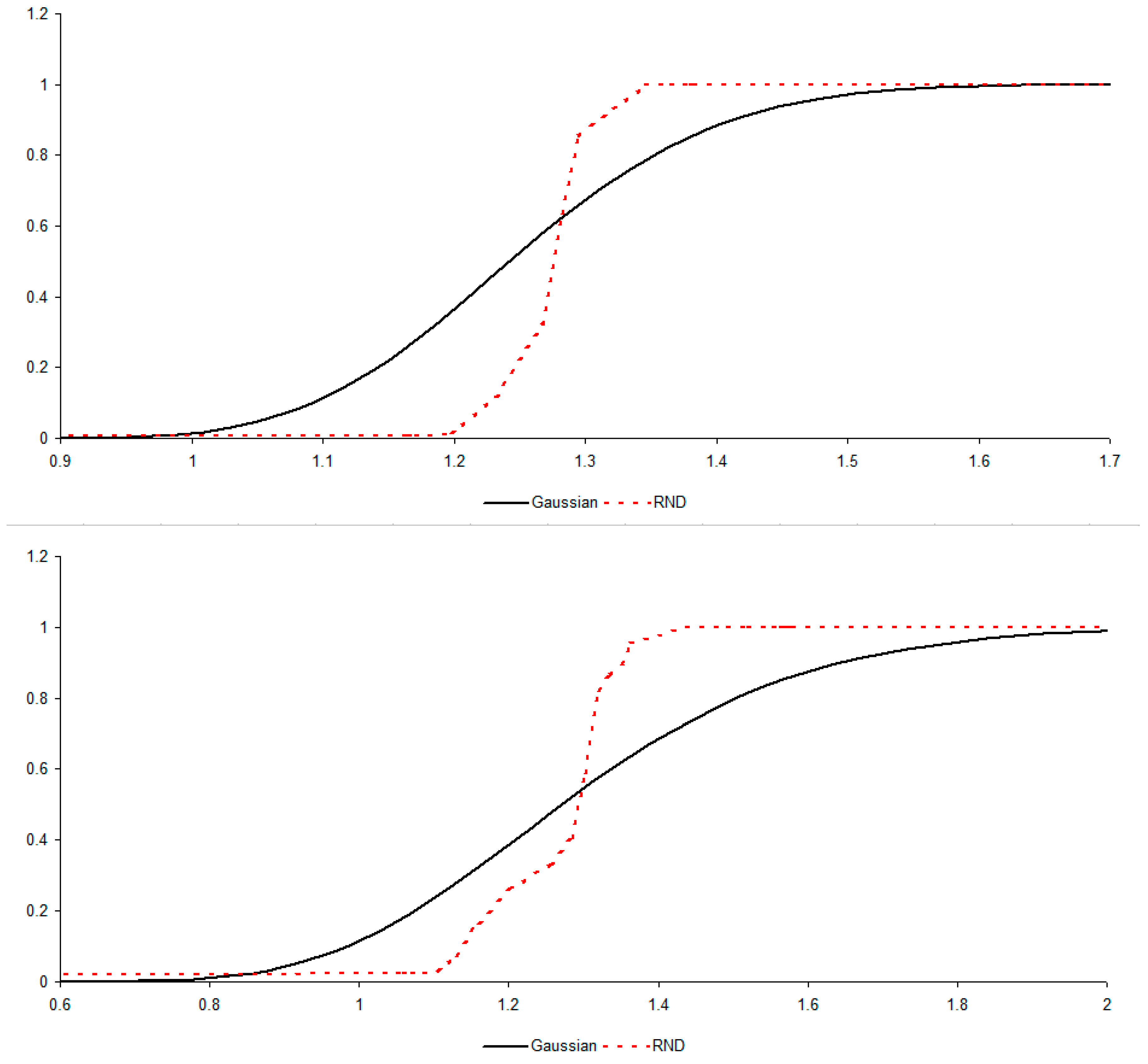
In addition to the density values, we also compute the upper limits of the density function ($x$) to be 1.382695 and 1.579103 for 3-month and 1-year maturities, respectively. We plot the RND results in Figure 6.

To apply the Gaussian copula, we need the Gaussian distributions at 3-month and 1-year timepoints. These Gaussian distributions are generated by the binomial model. We use 100 periods for the binomial lattice. Proportionally, the 3M option is priced by the distribution at $i=25$ and the 1Y options are priced by the distribution at $i=100$. In the lattice, we use the volatility of 19.78% for the first 3 months and 22.06% for the remaining 9 months. These volatility values are calibrated to the options to generate the minimal pricing errors by the lattice. For simplicity (and without loss of generality), we use a 0% interest rate. Figure 7 compares the two distributions.

Figure 7 provides the mappings from the RND functions to the Gaussian distributions of the two maturities. The task now is to derive the joint distribution between the two RND functions.

We assume 100 periods for the binomial model (derived in the Appendix A). Hence, at a three-month timepoint ($T_{\mathcal{l}}=0.25$), $i=25$, and at a one-year timepoint ($T_{\mathcal{l}+1}=1$), $i=100$. We know that at each timepoint, the (log) asset price distribution from the binomial model is Gaussian. The binomial lattice computes all the conditional probabilities. Hence, multiplying these conditional probabilities by the marginal probabilities at $i=25$, i.e., ${\underset{¯}{\pi }}_{25}$, we obtain the joint distribution between the two Gaussian distributions. This joint Gaussian distribution is then mapped to the RND functions to generate the joint distribution of the two RND functions. Following the steps described in Section 4, we can then plot the two joint distributions (for Gaussian and RND, respectively) in Figure 7.

In Figure 8, the blue dots depict the joint bi-variate Gaussian distribution implied by the binomial model, and the orange dots depict the joint distribution implied by the two RND functions.

Lastly, we can convert this joint distribution back to the conditional distribution by dividing the joint probabilities by multiplying by the RND marginal probabilities at $i=25$.11 These RND conditional probabilities can then be used to compute the expected payoffs of the option.

Now, we can compare the expected option payoffs (i.e., continuation values) against the exercise value and compute the Bermudan option price. We use put options as an example because for call options, the Bermudan value and European value are equal.

Take the 1Y ATM option as an example, the strike is 1.27260. The European put price is 0.05982. The Bermudan option is 0.06186. As a comparison, the binomial model has a European put price of 0.08049 and an American price of 0.08206.

Strike	1.049059	1.166820	1.272601	1.368343	1.467118
	1Y Put Option
RND Bermudan	0.012794	0.028410	0.061856	0.119404	0.205468
RND European	0.011143	0.026472	0.059823	0.117351	0.200594
BS Bermudan	0.014456	0.040229	0.082065	0.137326	0.211435
BS European	0.014452	0.040029	0.080494	0.131574	0.197970

In the above example, the Bermudan put options can be exercised only twice—once at maturity (one year) and once at the three-month timepoint. This is because European options are available only at these maturities (and hence, RNDs are available only on these dates). As a result, the Bermudan prices are uniquely defined. If the Bermudan options can also be exercised at 6M and 9M, then their prices cannot be uniquely defined by the two RNDs (or equivalently defined by the two sets of European options). A certain interpolation algorithm must be taken (i.e., fake option prices at 6M and 9M must be generated), and the Bermudan prices will vary with the chosen interpolation algorithm.

6. Conclusions and Future Research

In this paper, we propose a model-free lattice which is based upon the market prices of European options. European option prices of the same maturity (different strikes) can provide a risk-neutral density (RND) function on the maturity date. To build a lattice model that is consistent with multiple RND functions on various maturity dates, we use a Gaussian copula, which can be easily degenerated to a standard binomial model.

Our result makes a significant contribution to the literature in that the model-free lattice we derive in this paper is a description of a complete price evolution of the underlying asset. Similar to the Cox et al. (1979) binomial lattice, which is a description of the log-normal stock price process, our model-free lattice describes the whole evolution of the underlying asset and can accurately re-price all existing European options (across strikes and maturities) in the marketplace. In other words, our model-free lattice is a natural extension of Britten-Jones and Neuberger (2000), who restrict themselves to a random volatility process.

Given that our model-free lattice is consistent with all market option prices, it must embed all necessary risk factors (e.g., random volatility, random interest rates, and jumps) and market restrictions (e.g., mean-reversion and liquidity) that are priced into the European options. Our model-free lattice is a substantial improvement over the random volatility process by Britten-Jones and Neuberger (2000).

To see an easy implementation of our model-free lattice, we provide an example of a two-period FX option where European options are taken from 3-month and 1-year maturities. The European options provide RND functions which are mapped to each slice in the lattice. To finally complete the evolution (i.e., those transition probabilities in the lattice), a Gaussian copula is used.

Our model-free lattice is completely flexible and, hence, can be used for any asset class since it can adapt to any stochastic processes. The major output of our model is all of the transition probabilities. These transition probabilities could present a certain behavior (e.g., random volatility) that is not easily seen because the stochastic process the model-free lattice represents may not exist in a parametric form. Nevertheless, one can perform a series of statistical tests to study the properties (e.g., random volatility or mean-reversion) of the process. These properties could have important trading implications that can help investors predict market conditions and make investment decisions accordingly. We will leave this for future research.