Economic Resilience in Post-Pandemic India: Analysing Stock Volatility and Global Links Using VAR-DCC-GARCH and Wavelet Approach

Abstract

This study explores the resilience of the Indian stock market in the face of global shocks in the post-pandemic era, focusing on its volatility dynamics and interconnections with international indices. Through a combination of Vector Autoregression (VAR), DCC-GARCH, and wavelet analysis, we analysed the time-varying relationships between the National Stock Exchange (NSE) of India and major global indices, including those from the U.S., Europe, Asia-Pacific, Hong Kong and Japan. Time series data of the selected indices have been collected for the period 1 January 2021 to 30 September 2024. Results reveal that while the NSE demonstrates resilience through rapid adjustments following shocks, it remains vulnerable to substantial spillover effects from markets such as the S&P 500 and European indices. Wavelet coherence analysis identifies periods of high correlation, particularly during major economic events, indicating that regional and global factors can periodically compromise market stability. Moreover, the DCC-GARCH results show a persistent but fluctuating correlation with specific markets, reflecting a connected and adaptive nature of the Indian market that is influenced by regional dynamics. This study emphasises the importance of strategic risk management. It highlights critical periods and indices that policymakers and investors should monitor closely to understand the economic resilience of the Indian financial market better. Further research could explore sector-specific impacts and the role of macroeconomic factors in shaping market responses.

1. Introduction

The resilience of financial markets, particularly in emerging economies like India, has garnered significant attention in the wake of the COVID-19 pandemic (Hasan et al., 2022; Indrawati et al., 2020; Ray, 2023; Tiwary et al., 2022). As global financial systems faced unprecedented challenges, understanding how individual markets respond to international shocks became imperative. This research investigates whether the Indian stock market exhibits resilience compared to its global counterparts in the post-pandemic era, utilising advanced econometric models, namely VAR-BEKK-GARCH and wavelet analysis. Focusing on the interactions between the Indian market and various foreign indices, this study seeks to identify the nature and extent of spillover effects, contributing valuable insights to financial stability and risk management.

The research problem centres on verifying the ability of the Indian stock market to withstand external shocks and its interdependence with international markets. Over the past two decades, the study of return and volatility spillovers across stock market indices has become a prominent area of research, driven by both their practical implications and the inherently volatile nature of financial markets, which fluctuate over time (Bonga-Bonga & Phume, 2022; Booth et al., 1997; Mukherjee & Mishra, 2010; Yarovaya et al., 2016). The increasing globalisation of financial markets and rapid technological advancements have led to a deeper integration of emerging markets into the global economy, adding complexity to the interactions between markets. This integration has significant implications for portfolio management, as volatility spillovers can diminish the diversification benefits in emerging markets, complicating the management of international portfolios. Additionally, global crises, such as the Global Financial Crisis (GFC), the European Debt Crisis (EDC), trade tensions, the COVID-19 pandemic, and geopolitical conflicts, have spurred heightened academic interest in the contagion and interconnectedness of stock markets across different periods: before, during, and after these disruptions (Bhowmik & Wang, 2020; Dhingra et al., 2024; Maharana et al., 2024). While previous studies have explored the resilience of financial markets during crises, limited research has specifically addressed the post-pandemic recovery phase and its implications for the Indian market (Maharana et al., 2024; Tiwary et al., 2022). This study aims to fill this gap by applying a multifaceted analytical framework incorporating time-series econometrics and wavelet transforms. Doing so will provide a better understanding of market dynamics, helping investors and policymakers assess the potential vulnerabilities and strengths of the Indian financial system in a rapidly changing global environment.

This research addresses the need for robust financial frameworks in emerging economies, where the repercussions of global shocks can be particularly pronounced in recent times. Understanding the resilience of the Indian economy in a period of political stability, increased global reach, and bilateral relations not only aids investors in making better decisions but also equips policymakers with the necessary tools to enhance regulatory frameworks and safeguard against future crises. As the global economy continues to evolve, insights from this study will contribute to the ongoing discourse on financial stability and economic resilience, ultimately promoting sustainable growth in the Indian context.

2. Literature Review

The mechanisms of international information transmission between markets, evident through both returns and volatility, hold significant theoretical and practical importance. Volatility spillovers occur when fluctuations in one market incite similar volatility in others, which becomes especially pronounced during market turmoil, reducing the advantages of international portfolio diversification for investors. This effect has been intensified by recent technological advancements, which have improved domestic investors’ access to global information and accelerated information flow between markets. Examining return and volatility spillovers across stock markets in various geographical regions is crucial, enhancing our understanding of international financial interconnectedness.

The resilience of financial markets, particularly in the context of global economic disruptions, has been a topic of increasing scholarly interest in recent years (He, 2001; Jin & An, 2016; H. Liu et al., 2022; Maharana et al., 2024; Mishra et al., 2022). Resilience is often defined as the ability of a market to absorb shocks and recover from disturbances while maintaining its fundamental functions (Choptiany et al., 2021). Research has shown that emerging markets, like India, face unique challenges and vulnerabilities compared to developed markets, particularly during crises such as the COVID-19 pandemic (Arfaoui & Yousaf, 2022; Chaudhary et al., 2020; Malik et al., 2022; Thangamuthu et al., 2022). Several studies have highlighted the importance of understanding these dynamics to formulate effective risk management strategies (Chaudhary et al., 2020; Maharana et al., 2024; Thangamuthu et al., 2022).

A significant body of literature has explored the concept of market resilience through various analytical frameworks. For instance, the application of econometric models such as Vector Autoregression (VAR) and Generalised Autoregressive Conditional Heteroskedasticity (GARCH) has become commonplace in assessing the interdependencies and volatility spillovers between markets (Arfaoui & Yousaf, 2022; Karolyi, 1995; Maharana et al., 2024; Singhal & Ghosh, 2016; Yadav et al., 2023). VAR models allow for examining the dynamic relationships among multiple time series, making it possible to understand how shocks in one market can influence another. GARCH models, on the other hand, provide insights into the volatility clustering phenomenon often observed in financial time series data. The combination of VAR and GARCH frameworks, particularly the BEKK-GARCH specification, has proven effective in capturing the complexities of multivariate time series data and elucidating the spillover effects between different markets (Karolyi, 1995; Maharana et al., 2024; Singhal & Ghosh, 2016).

In recent years, the application of wavelet analysis has emerged as a powerful tool for analysing the time-frequency characteristics of financial data (Armah et al., 2022; D. Liu et al., 2023; Rhif et al., 2019; Ye et al., 2020). Unlike traditional time series methods, wavelet transforms enable researchers to examine how relationships between financial markets evolve over different time scales (Armah et al., 2022). Studies such as those by Baruník and Křehlík (2018) demonstrate that wavelet coherence can reveal significant insights into the dynamic correlations between stock markets during periods of crisis. This method is particularly relevant in the context of the COVID-19 pandemic, as it identifies time-varying dependencies that static models may not capture. By integrating wavelet analysis with GARCH models, researchers can attain a more comprehensive understanding of market resilience and the intricate web of interactions between emerging and developed economies (Sifuzzaman et al., 2009; Wang, 2021).

The COVID-19 pandemic has served as a catalyst for a renewed examination of financial market resilience, with numerous studies focusing on its impacts. For example, research by Y. Liu et al. (2022) has shown that the pandemic-induced market volatility affected emerging markets more severely than developed ones. This disparity can be attributed to factors such as lower liquidity, heightened investor sentiment, and greater reliance on foreign investments. Additionally, studies have indicated that markets in developing countries often exhibit higher sensitivity to global economic shocks due to their interconnectedness with developed markets (Jin & An, 2016; Maharana et al., 2024; Mishra et al., 2022). Similarly, India’s post-pandemic financial market volatility has shown both resilience and challenges (Maharana et al., 2024). While the Indian market experienced significant volatility, it has managed to recover and adapt, supported by robust policy measures and economic reforms.

On the other hand, global markets have also faced volatility but have benefited from a more synchronised monetary policy response and stronger financial safety nets (Adrian, 2020). The Indian market’s recovery has been uneven, with sectors like agriculture and manufacturing showing resilience. In contrast, others, such as retail and services, have gradually bounced back (Tamhane, 2020). The Indian stock market, as one of the largest in the emerging market space, provides a unique case study for analysing these dynamics, particularly as it navigates the recovery phase post-pandemic.

Moreover, the literature on financial market integration portrayed the significance of understanding cross-border interactions in the context of resilience. For instance, Eun and Resnick (1984) established that financial markets are increasingly interconnected, with information flows and capital movements influencing market behaviour (Giudici et al., 2020; Raddant & Kenett, 2021). Recent studies have built on this foundation, highlighting the importance of analysing not only the direct relationships between markets but also the spillover effects of macroeconomic shocks (Aggarwal & Jha, 2023; Mohanasundaram et al., 2024; Raddant & Kenett, 2021).

Research on volatility spillover between global financial markets has highlighted the increasing interconnectedness and complex dynamics among various asset classes and regions, especially during times of crisis. Jebabli et al. (2022) examined data from MSCI World, Emerging, and European stock markets, revealing that the COVID-19 pandemic caused significant volatility spillover, with a pattern distinct from that observed during the 2008 financial crisis. Similarly, Khan (2024) and Li (2021) explored the volatility transmission between developed and emerging markets, finding that developed markets primarily drive volatility spillover to emerging markets, underscoring the dominant influence of mature economies on the stability of developing ones. Shahzad et al. (2021), focusing on China’s stock market across various sectors, observed that the negative impact of volatility spillovers exceeded the positive effects during the COVID-19 pandemic, suggesting a heightened need for investor caution. Erdoğan et al. (2020) studied the period between 2013 and 2019 to assess volatility transmission from the Islamic stock market index to foreign exchange rates in India, Turkey, and Malaysia, finding a significant spillover from the Turkish Islamic index to exchange rates, while other nations exhibited limited effects.

Further studies on regional volatility interactions have also provided valuable insights for investment strategies. Using the DCC-GARCH technique, Zhong and Liu (2021) examined the volatility spillover between Chinese and Southeast Asian stock markets, concluding that portfolio diversification across these countries could reduce risk. Sarwar et al. (2020) investigated the relationship betwen oil market volatility and stock market indexes in India, Pakistan, and China, finding that volatility consistently spills from the oil market to stock markets in these regions, limiting the effectiveness of oil assets as tools for diversification in these economies. Together, these studies underscore the importance of understanding cross-market spillovers in asset-specific and broader regional contexts, as they carry significant implications for investors and policymakers aiming to mitigate risks and design resilient investment portfolios.

Research on volatility in financial markets frequently references the GARCH family of models to capture the persistence of volatility shocks. In the past decade, many such studies have focussed on the interdependencies using various indices of groups of nations, including the influence of oil prices, exchange rates, etc. Kishor and Singh (2014) explore the relationship between stock return volatility in BRICS economies and external influences, mainly focusing on the 2008 financial crisis and its effects from 2007 to 2013. They observed that, with the exceptions of Brazil and China, the stock markets of BRICS countries are significantly influenced by U.S. market movements, highlighting substantial differences in volatility among these economies. Similarly, Tripathy (2022) addresses this subject by examining the stock markets of Brazil, Russia, India, China, and South Africa (BRICS) through advanced econometric modelling, including the GARCH, APARCH, ARFIMA, and FIGARCH frameworks. The results reveal significant volatility persistence, as evidenced by the GARCH model. At the same time, APARCH findings indicate leverage effects, meaning adverse shocks impact volatility more than positive ones. Additionally, ARFIMA and FIGARCH models confirm long-range dependence in returns and volatility, challenging the Efficient Market Hypothesis (EMH) by suggesting that market behaviour in these countries may be somewhat predictable over time.

While numerous studies have explored volatility spillovers and market interdependencies, especially in the context of global crises like the 2008 financial crash and the COVID-19 pandemic, there remains a critical gap in understanding the resilience of the Indian stock market in the post-COVID era relative to major global indices. Existing research often focuses on either emerging markets broadly or developed economies individually. Likewise, many researchers have considered different groups of countries, such as BRICS, G7, G20, META, etc., to verify their market interdependency of volatility in return and time dependency. Yet few studies specifically address how the Indian stock market, as a prominent emerging market, responds to shocks compared to key global indices such as NSE, AAXJ, STOXX, GSPC, FTSE, N225, and HSI. This study addresses this gap by employing advanced econometric techniques, including VAR, multivariate GARCH, and wavelet analysis, to provide a detailed assessment of cross-market dependencies and resilience. By focusing on the unique dynamics of the Indian stock market’s interactions with global counterparts, this research aims to contribute to the literature on emerging market resilience and inform policymakers and investors about the robustness of the Indian market in a post-pandemic global landscape.

3. Data and Methodology

3.1. Data

Studying the resilience of Indian stock indices in the post-COVID era, particularly amidst ongoing geopolitical tensions such as the Russia–Ukraine conflict and instability in the Middle East, is highly justifiable as it reflects the complex interplay between global events and market dynamics. These conflicts have profound implications for global supply chains, energy prices, and investor sentiment, creating uncertainty that can significantly affect emerging markets like India. By examining the Indian stock market in this context, we can gain insights into how domestic equities respond to external shocks and geopolitical risks, revealing the underlying strengths and vulnerabilities of the Indian economy. Additionally, understanding this resilience is vital for policymakers and investors seeking to navigate the intricacies of a rapidly changing global landscape, thereby enhancing strategic decision-making and risk management in an increasingly interconnected world. This study contributes to academic discourse and provides practical implications for stakeholders concerned about financial stability and growth in turbulent times.

In selecting the Nifty 50, MSCI Asia ex-Japan Index, STOXX Europe 600, S&P 500, FTSE 100, Nikkei 225, and Hang Seng Index as per the details given in

Table 1. Indices used for the study.

Index Name	Region	Ticker Code
Nifty 50	India	NSE
MSCI Asia ex-Japan Index	Asia-Pacific	AAXJ
STOXX Europe 600	Europe	STOXX
S&P 500	USA	GSPC
FTSE 100	United Kingdom	FTSE
Nikkei 225	Japan	N225
Hang Seng Index	Hong Kong	HSI

, the objective is to provide a comprehensive analysis of global financial market resilience in the post-COVID era. Each index represents vital economic regions and diverse market characteristics, capturing a broad performance spectrum across developed and emerging markets. The Nifty 50 serves as a benchmark for the Indian market, and the MSCI Asia ex-Japan Index allows for a focused examination of regional trends in Asia, reflecting the dynamics of major economies in the area. The STOXX Europe 600 and FTSE 100 represent the European market landscape, encompassing large-cap companies from various sectors. At the same time, the S&P 500, Nikkei 225, and Hang Seng Index provide critical perspectives from the United States, Japan, and Hong Kong, respectively. We have not included the ACWI (All Country World Index) and EEM (Emerging Markets) like indices since they highly correlate with GPSC and AAXJ, respectively, to avoid model-building issues. By analysing these indices together, we try to uncover the interconnectedness and spillover effects within and across markets, enhancing our understanding of the global financial landscape in the wake of the pandemic.

The selection of the study period, from 1 January 2021 to 30 September 2024, focuses on the post-pandemic era, a crucial phase in global economic recovery. It can be observed from Figure 1 that there was a steep fall in the stock market indices during COVID-19, and almost all indices had recovered entirely from this blood bath by the first quarter of 2021. From April 2021, the world witnessed the initial recovery phase from the COVID-19 pandemic as vaccination efforts ramped up and economies gradually reopened. This period captures the effects of various fiscal and monetary policies implemented globally to mitigate the pandemic’s impact. Moreover, it coincides with significant global events such as supply chain disruptions, inflationary pressures, the Russia–Ukraine war, and ongoing geopolitical tensions in the Middle East. These factors make this period ideal for assessing the resilience of the Indian stock market to external shocks, providing insights into how it has adapted to a volatile post-pandemic global environment. The end of September 2024 marks a suitable cutoff to include recent developments and capture mid-term economic responses to these global shocks.

3.2. Method

VAR (Vector Autoregression) Model: Using the Augmented Dickey–Fuller (ADF) test, we verified the stationarity of the return series. Then, we verified the Akaike information criterion (AIC) or Schwarz Bayesian Criterion (SBC) to determine the optimal lag length for the VAR model. The next step is to fit a VAR model using the selected lag length. The VAR model can be represented as:

$$Y_t=c+A_1{Y}_{\left\{t-1\right\}}+A_2{Y}_{\left\{t-2\right\}}+\dots +A_p{Y}_{\left\{t-p\right\}}+{ϵ}_t$$

where $Y_t$ is the vector of returns, ccc is a vector of constants, Ai are the coefficient matrices, and ${ϵ}_t$ is the vector of error terms.

Impulse Response Functions (IRFs): Analyse how shocks to one index affect others over time using IRFs, which can be computed after estimating the VAR model.

Diebold–Yilmaz Spillover Index: The Diebold–Yilmaz spillover index method quantifies the extent of interconnectedness and volatility spillovers across financial markets (Diebold & Yilmaz, 2009). It begins with estimating a Vector Autoregressive (VAR) model for the returns of the selected indices, capturing their dynamic relationships. The next step involves calculating the Forecast Error Variance Decomposition (FEVD), which partitions each variable’s total forecast error variance (index) into contributions from shocks to itself and other indices. The Diebold–Yilmaz spillover index is then computed using these variance decompositions, measuring the proportion of the forecast error variance of one index attributable to shocks in other indices. The index aggregates these cross-market contributions to reflect the total spillover effect within the system, providing a quantitative assessment of how market shocks propagate across different indices. The Diebold–Yilmaz spillover index is estimated using the following equations:

$$TotalSpillover={\displaystyle \frac{{\sum }_{i\ne j}{\sigma }_{ij}^2}{{\sum }_{i=1}^n{\sigma }_{ii}^2}}$$

where ${\sigma }_{ij}^2$ is the forecast error variance attributable to shocks from variable ‘j’ to variable ‘i’, and ‘n’ is the number of variables.

The Univariate GARCH Estimation: For each time series (index), estimate a univariate GARCH model. A common choice is the GARCH (1,1) model, which can be expressed as:

$$R_t=\mu +{ϵ}_t$$

where ${ϵ}_t={\sigma }_t{z}_t \mathrm{a}\mathrm{n}\mathrm{d} z_t~\mathcal{N}\left(0,1\right)$ (standard normal distribution).

Suppose the results of the GARCH (1,1) model diagnostics for autocorrelation are not satisfied; it requires further adjustments of leg structure or the adoption of complex models like BEKK-GARCH (Bollerslev, 1986; Hafner et al., 2022; Tsay, 2010).

The GARCH (1,1) model for the conditional variance ${\sigma }_t^2$ is given by:

$${\sigma }_t^2={\alpha }_0+\sum _{i=1}^p{\alpha }_i{ϵ}_{t-i}^2+\sum _{j=1}^q{\beta }_j{\sigma }_{t-j}^2$$

In this framework, $R_t$ is the return at time t, μ is the mean return, ${ϵ}_t$ is the innovation or shock at time $t,z_t$ is a standard normal variable, ${\sigma }_t$ is the conditional variance, and ${\alpha }_0,{\alpha }_i,{\beta }_j$ are parameters that need to be estimated. The first step is to fit a univariate GARCH model for each asset’s returns to capture their volatility dynamics. Use Maximum Likelihood Estimation (MLE) to estimate the parameters ω, α, and β for each univariate GARCH model.

DCC-GARCH Model: The Dynamic Conditional Correlation Generalised Autoregressive Conditional Heteroskedasticity (DCC-GARCH) model is a powerful econometric technique for analysing time-varying correlations between multiple financial time series. This model extends the standard GARCH approach by allowing the conditional correlations between assets to vary over time, capturing dynamic relationships more flexibly. The DCC-GARCH model operates in two steps: first, univariate GARCH models are fitted to each series to estimate conditional variances; then, a dynamic correlation matrix can be calculated using standardised residuals from these GARCH models. This two-step approach helps identify how correlations evolve in response to market events, which is crucial for understanding volatility spillovers and portfolio risk management. The DCC-GARCH model is prevalent for financial market analysis because it captures the co-movement of assets in a dynamic and time-sensitive manner, making it helpful in assessing interconnected risks and market dependencies (Engle, 2002). The DCC model is specified as follows:

Conditional Correlation: $Q_t=\left(1-\alpha -\beta \right)\overline{Q}+\alpha {\widehat{z}}_{t-1}{z}_{t-1}^{’}+\beta Q_{t-1}$.

In this equation, $Q_t$ is the conditional correlation matrix, $\overline{Q}$ is the unconditional correlation matrix of the residuals, while α and β are parameters that control the weights of the previous correlations and residuals, respectively, with α, β ≥ 0 and α + β < 1. The DCC model effectively captures how correlations change over time based on the lagged information from the standardised residuals.

Wavelet Coherence (WCOH): WCOH complements the analyses by quantifying the local correlation between the Indian stock market and selected global indices over time and frequency. This method helps assess how the strength of the relationship between the Indian market and global indices varies during different market conditions (Grinsted et al., 2004; Torrence & Compo, 1998).

The mathematical formulation of WCOH is as follows:

$$WCOH\left(a,b\right)={\displaystyle \frac{{\left|XWT\left(a,b\right)\right|}^2}{{\left|W_1\left(a,b\right)\right|}^2{\left|W_2\left(a,b\right)\right|}^2}}$$

where W₁ and W₂ are the wavelet transforms of the individual time series. The WCOH provides insights into the strength and significance of the correlation between the series at various scales and time points.

4. Observations

4.1. Descriptive Statistics

It can be noted from

Table 2. Descriptive statistics using the daily return data (N = 975).

	AAXJ	FTSE	GSPC	HSI	N225	NSE	STOXX
Mean	−0.0102	1.9080	2.0329	−6.7680	12.7030	12.4723	0.1311
Median	0.0000	2.8999	1.0801	0.0000	0.8301	6.6992	0.3100
Maximum	6.3300	282.5000	207.8000	1672.4199	3217.0410	735.8496	19.4400
Minimum	−2.9300	−292.6001	−177.7202	−1129.6602	−4451.2793	−1379.4004	−20.3300
Std. Dev.	0.9091	59.2137	44.1972	315.2880	400.5728	161.6786	3.9330
Skewness	0.2876	−0.4683	−0.3000	0.2458	−1.1234	−0.7832	−0.5158
Kurtosis	6.0496	6.3379	4.4828	4.9666	23.5536	10.5541	5.8549
Jarque–Bera	391.2647 *	488.2601 *	103.9430 *	166.9356 *	17367.0813 *	2417.9006 *	374.3457 *

* Indicates significance level at p-values less than 0.01.

that the means return range widely, with N225 (12.7030) and NSE (12.4723) showing the highest average returns, while AAXJ has a slight negative mean (−0.0102), suggesting a slight downward trend. The median values vary, with several indices like AAXJ, HSI, and STOXX at zero, indicating a high occurrence of neutral or zero returns. Notably, the maximum and minimum values for N225 and NSE reveal extreme fluctuations, with N225 reaching a peak of 3217.0410 and a low of −4451.2793, signifying high volatility. Standard deviations confirm this volatility, with N225 and NSE exhibiting substantial variability (400.5728 and 161.6786, respectively). Skewness values suggest that most distributions are slightly left-skewed, except for AAXJ and HSI, which show mild right-skewness, implying asymmetry and occasional more significant positive or negative returns. The high kurtosis values, especially for N225 (23.5536) and NSE (10.5541), suggest heavy-tailed distributions, indicating more frequent extreme returns than a normal distribution. The significant Jarque–Bera statistics confirm that none of the indices returns follow a normal distribution, primarily due to their skewed and leptokurtic nature.

Table 3. Unit root tests.

	Augmented Dickey–Fuller Test (ADF)				Phillips–Perron Test (PP)
	Level		At First Difference		Level		At First Difference
Variables	t-Statistic	Prob.	t-Statistic	Prob.	t-Statistic	Prob.	t-Statistic	Prob.
AAXJ	−0.9892	0.944	−33.1635	0.000	−0.8426	0.960	−33.1860	0.000
FTSE	−4.2177	0.004	−32.3240	0.000	−4.1083	0.006	−32.4989	0.000
GSPC	−1.2474	0.899	−31.0539	0.000	−1.1450	0.920	−31.0933	0.000
HSI	−1.7887	0.710	−14.4577	0.000	−1.7048	0.749	−30.5488	0.000
N225	−2.1363	0.524	−31.9512	0.000	−2.0807	0.555	−31.9512	0.000
NSE	−1.2831	0.891	−32.1889	0.000	−1.1496	0.919	−32.2478	0.000
STOXX	−2.3116	0.427	−19.5721	0.000	−2.2092	0.483	−31.3784	0.000

presents the Augmented Dickey–Fuller (ADF) and Phillips–Perron (PP) tests for stationarity, revealing consistent results across the variables. At the level (original form), none of the indices (except FTSE in both ADF and PP tests) are stationary, as indicated by high p-values (greater than 0.05). This suggests the presence of a unit root, implying non-stationarity in most of the indices at their levels. However, when differenced once, all variables become stationary, evidenced by highly significant p-values (0.000) in both ADF and PP tests, meaning they reject the null hypothesis of a unit root at the first difference.

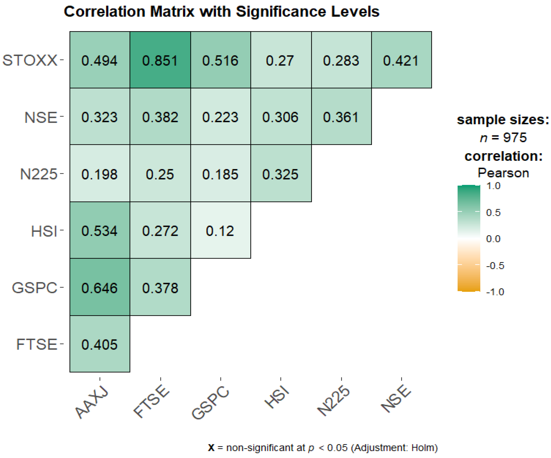
The correlation matrix in Figure 2 shows varying degrees of association among the indices. All the correlation values are positive and significant at p-values less than 0.01. The strength of correlation between two variables indicated with a relatively darker shed of the green colour for positive correlation and orange colour for negative correlation. The STOXX index strongly correlates with FTSE (0.851) and GSPC (0.516), indicating a high positive association with these markets, likely reflecting regional economic connections. AAXJ is moderately correlated with GSPC (0.646) and STOXX (0.494), suggesting it somewhat moves with these global indices. FTSE and NSE also exhibit moderate correlations with each other (0.382) and STOXX, reflecting potential interdependencies. N225, however, has generally low correlations with the other indices, indicating weaker co-movement with global markets, possibly due to regional market dynamics unique to Japan. While specific indices like STOXX and FTSE show strong relationships, others, particularly N225, have more isolated movement patterns. In contrast, NSE shows a moderate correlation with the other global indices.

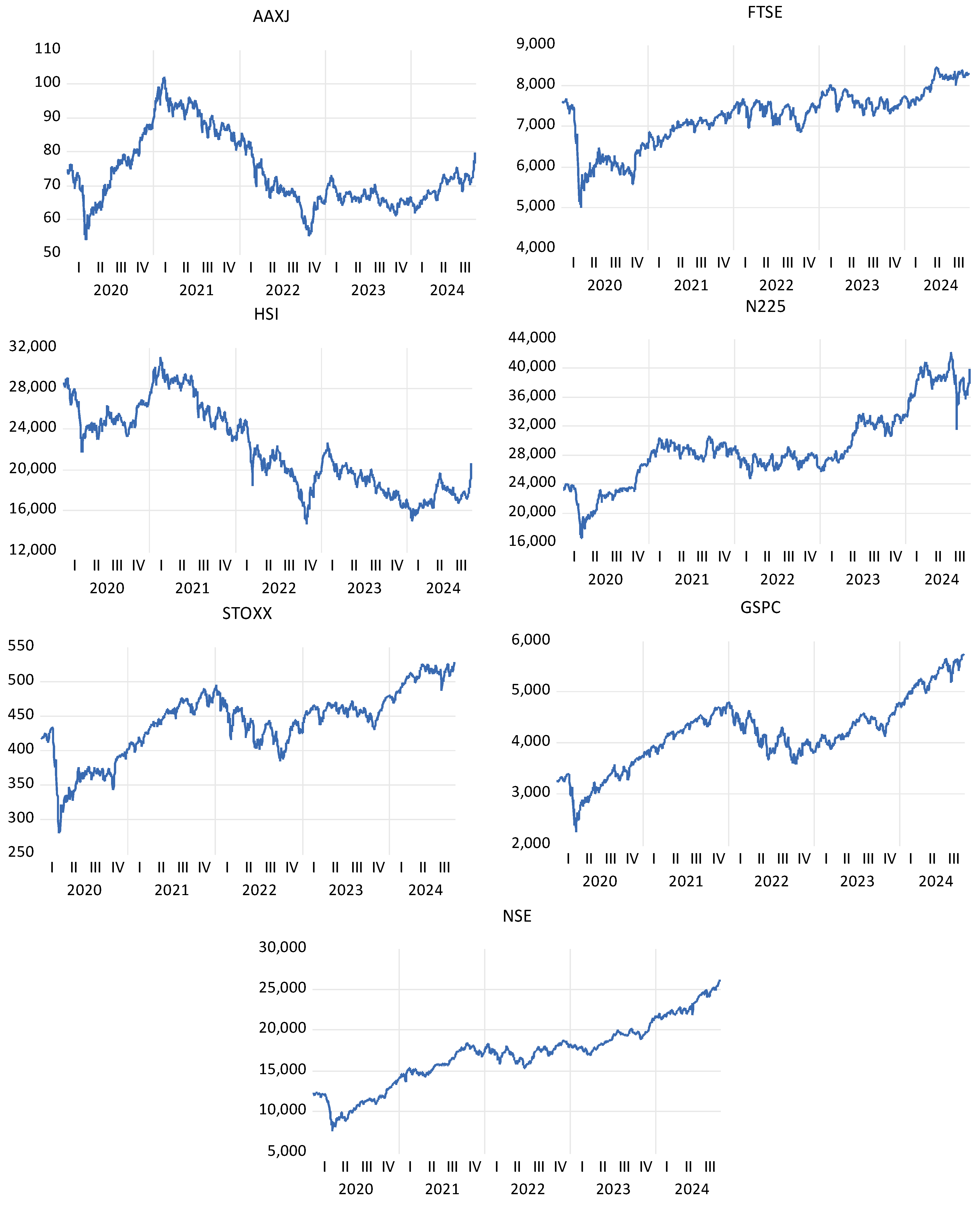
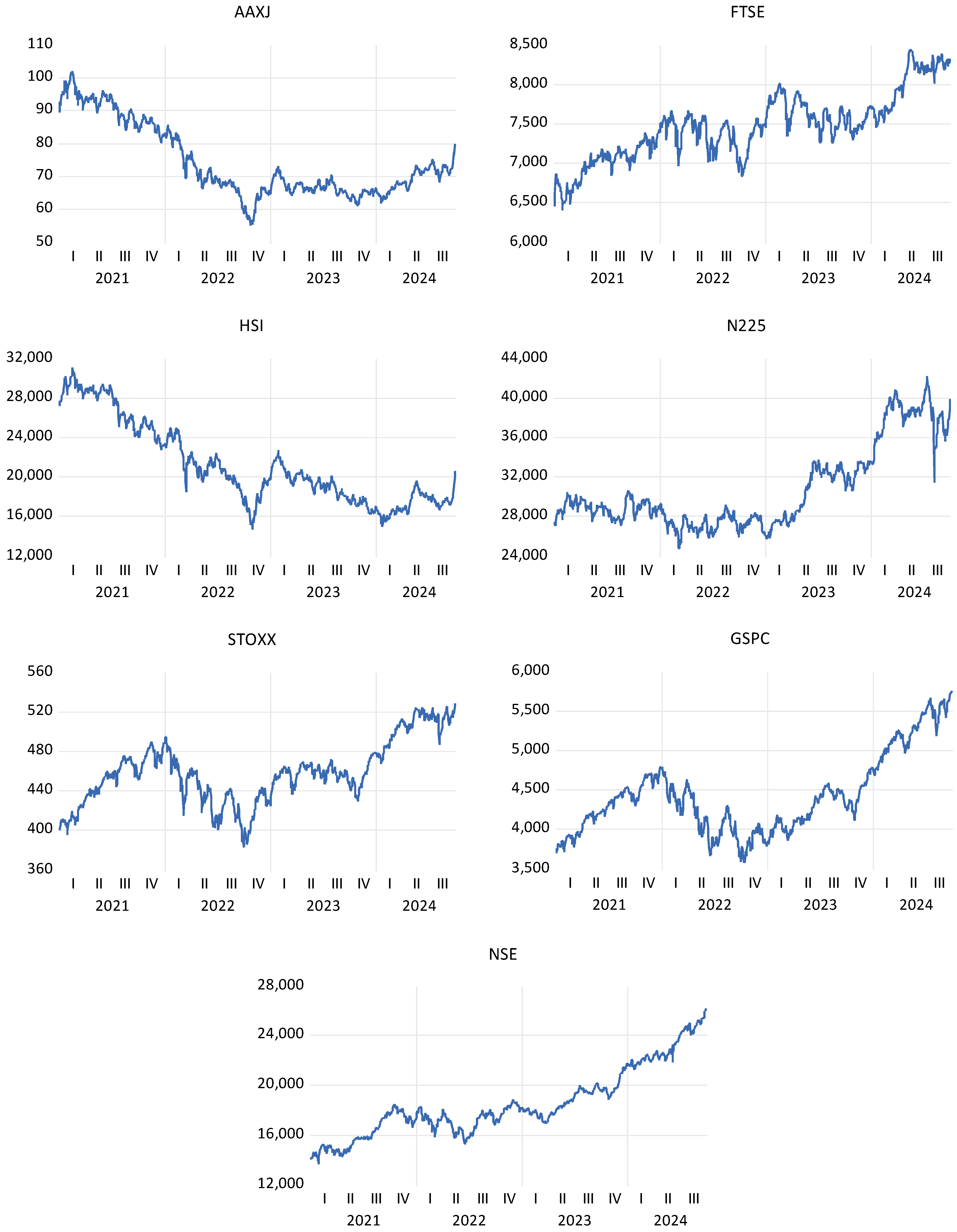
Figure 3 and Figure 4 illustrate the trend of the daily closing prices and log differentiated returns of the selected global indices for the post-pandemic period. FTSE and NSE show a rising trend, whereas AAXJ and HIS show a declining trend in the post-pandemic period. On the other hand, STOXX, N225, and GSPC recorded growth after the 4th quarter of 2022.

4.2. The VAR Model

The VAR results in

Table 4. VAR model.

		AAXJ	FTSE	GSPC	HSI	N225	NSE	STOXX
AAXJ(−1)	Coeff.	−0.03829	0.050133	0.007312	0.756044	0.080821	0.09667	0.006091
	SE	0.059321	0.038345	0.050617	0.067094	0.053885	0.041468	0.041139
	t	[−0.64551]	[1.30739]	[0.14445]	[11.2685]	[1.49987]	[2.33120]	[0.14806]
AAXJ(−2)	Coeff.	0.140704	0.042043	0.093127	0.306489	0.040286	0.099995	0.05417
	SE	0.059262	0.038307	0.050566	0.067026	0.053831	0.041426	0.041098
	t	[2.37429]	[1.09753]	[1.84168]	[4.57267]	[0.74838]	[2.41379]	[1.31807]
FTSE(−1)	Coeff.	−0.05274	0.01693	−0.06601	0.117186	−0.24365	−0.004	0.08628
	SE	0.094431	0.061041	0.080576	0.106804	0.085778	0.066011	0.065488
	t	[−0.55851]	[0.27736]	[−0.81920]	[1.09721]	[−2.84044]	[−0.06057]	[1.31750]
FTSE(−2)	Coeff.	0.007491	0.010076	0.02965	0.069441	0.155993	−0.03754	0.013907
	SE	0.094077	0.060812	0.080274	0.106404	0.085456	0.065764	0.065243
	t	[0.07962]	[0.16569]	[0.36937]	[0.65262]	[1.82541]	[−0.57078]	[0.21315]
GSPC(−1)	Coeff.	−0.05052	0.188798	−0.02646	−0.15976	0.408374	0.206909	0.291335
	SE	0.057997	0.03749	0.049488	0.065596	0.052683	0.040543	0.040221
	t	[−0.87105]	[5.03601]	[−0.53477]	[−2.43547]	[7.75158]	[5.10350]	[7.24331]
GSPC(−2)	Coeff.	−0.12129	0.033102	−0.12018	0.015827	0.134225	0.021069	0.025325
	SE	0.061161	0.039535	0.052187	0.069175	0.055557	0.042754	0.042415
	t	[−1.98306]	[0.83728]	[−2.30284]	[0.22879]	[2.41601]	[0.49278]	[0.59708]
HSI(−1)	Coeff.	−0.02553	−0.01537	0.005573	−0.3616	−0.02266	−0.07224	−0.01666
	SE	0.039257	0.025376	0.033497	0.044401	0.03566	0.027442	0.027225
	t	[−0.65037]	[−0.60577]	[0.16637]	[−8.14387]	[−0.63544]	[−2.63235]	[−0.61192]
HSI(−2)	Coeff.	−0.09796	−0.03484	−0.08114	−0.15405	0.017166	−0.04676	−0.06288
	SE	0.035181	0.022741	0.030019	0.039791	0.031957	0.024593	0.024398
	t	[−2.78445]	[−1.53212]	[−2.70292]	[−3.87154]	[0.53714]	[−1.90126]	[−2.57710]
N225(−1)	Coeff.	0.054537	0.006983	−0.00284	−0.0294	−0.17047	−0.01053	0.001618
	SE	0.037685	0.02436	0.032155	0.042622	0.034231	0.026343	0.026134
	t	[1.44718]	[0.28667]	[−0.08842]	[−0.68973]	[−4.97997]	[−0.39986]	[0.06192]
N225(−2)	Coeff.	0.062819	−0.01293	0.036381	0.041528	−0.01689	0.007454	−0.00115
	SE	0.035114	0.022698	0.029962	0.039715	0.031896	0.024546	0.024352
	t	[1.78898]	[−0.56964]	[1.21425]	[1.04564]	[−0.52964]	[0.30369]	[−0.04704]
NSE(−1)	Coeff.	−0.11548	−0.02573	−0.06922	−0.23541	−0.09876	−0.1104	−0.02223
	SE	0.051561	0.033329	0.043996	0.058317	0.046836	0.036043	0.035758
	t	[−2.23974]	[−0.77197]	[−1.57326]	[−4.03680]	[−2.10869]	[−3.06304]	[−0.62160]
NSE(−2)	Coeff.	−0.09604	−0.05979	−0.08803	−0.12817	−0.01354	−0.04698	−0.05673
	SE	0.051135	0.033054	0.043632	0.057834	0.046449	0.035745	0.035462
	t	[−1.87820]	[−1.80902]	[−2.01748]	[−2.21614]	[−0.29159]	[−1.31437]	[−1.59985]
STOXX(−1)	Coeff.	0.160792	−0.19343	0.123431	0.130812	0.469441	0.051938	−0.25588
	SE	0.097254	0.062865	0.082984	0.109997	0.088342	0.067984	0.067446
	t	[1.65332]	[−3.07691]	[1.48740]	[1.18924]	[5.31391]	[0.76397]	[−3.79389]
STOXX(−2)	Coeff.	0.040734	−0.02765	0.074089	0.064007	−0.18667	0.023602	−0.03722
	SE	0.097879	0.063269	0.083518	0.110704	0.08891	0.068421	0.067879
	t	[0.41617]	[−0.43702]	[0.88711]	[0.57819]	[−2.09955]	[0.34495]	[−0.54834]
C	Coeff.	−5.65 × 10−5	0.000243	0.000539	−0.00013	0.000245	0.000605	0.000228
	SE	0.000393	0.000254	0.000335	0.000444	0.000357	0.000274	0.000272
	t	[−0.14381]	[0.95566]	[1.60964]	[−0.29931]	[0.68612]	[2.20585]	[0.83836]

Source: Authors own interpretation.

offer insights into the dynamic relationships among the indices. Based on the VAR lag selection criteria in

Table 5. Leg length selection criteria.

Lag	LogL	LR	FPE	AIC	SC	HQ
0	22,716.97	NA	9.42 × 10−30	−46.9700	−46.9347	−46.9565
1	23,099.45	758.6143	4.72 × 10−30	−47.6597	−47.3773 *	−47.5522 *
2	23,165.23	129.5204	4.56 × 10−30 *	−47.6943 *	−47.1651	−47.4929
3	23,210.64	88.75905	4.60 × 10−30	−47.687	−46.9107	−47.3914
4	23,253.63	83.39746 *	4.66 × 10−30	−47.6745	−46.6513	−47.2850
5	23,285.26	60.90666	4.83 × 10−30	−47.6386	−46.3684	−47.1550

* Indicates lag order selected by the criterion, LR: sequential modified LR test statistic (each test at 5% level); FPE: Final prediction error; AIC: Akaike information criterion; SC: Schwarz information criterion; HQ: Hannan–Quinn information criterion.

, lag two is chosen for interpretation according to the AIC. However, both lags are considered in the analysis, as the SC and HQ criteria recommend selecting lag 1. Notably, the lagged values of AAXJ exhibit a strong positive influence on HSI, with AAXJ(−1) showing a highly significant effect on HSI (11.2685), implying that past values of AAXJ have a substantial influence on HSI. Similarly, GSPC(−1) strongly impacts multiple indices, including FTSE (5.0360), N225 (7.7516), NSE (5.1035), and STOXX (7.2433), suggesting that U.S. market movements significantly affect these indices, particularly N225. FTSE(−1) shows a negative and significant effect on N225, indicating that FTSE declines could negatively impact N225. NSE(−1) is also influential, with adverse and significant effects on HSI and NSE, highlighting internal momentum within the NSE index. STOXX(−1) influences N225 (5.3139), pointing to the interdependence between European and Japanese markets.

The impulse response graphs given in Figure 5 illustrate how the National Stock Exchange (NSE) reacts to unexpected shocks or innovations from eight global indices over 10 days. Each plot provides insight into the NSE’s sensitivity to a one-standard-deviation innovation originating from a particular international market. Observing these responses helps us understand the degree and duration of influence that global market events have on the NSE and the stability of these influences over time.

In most cases, the immediate response of the NSE to a shock from a global index is noticeable within the first one to three days. For instance, indices like AAXJ (Asia ex-Japan) and FTSE (UK) appear to have a substantial initial impact, with the response of the NSE spiking within this early timeframe. This suggests that the NSE is highly responsive to sudden changes in these indices, possibly due to economic ties, trading patterns, or investor sentiment linked to these regions. However, after this initial surge, the response generally starts to decline, indicating that while the NSE reacts quickly to foreign market shocks, this reaction is often short-lived.

The prompt decline also reflects how rapidly the NSE adjusts to these external factors, with the impact fading as the local market absorbs and processes the new information. In contrast, indices like the N225 (Japan) and STOXX (Europe) exhibit a smaller initial impact, indicating a more limited influence on the NSE. GSPC (S&P 500) also shows a noticeable impact, though slightly less intense, which reflects the influence of the global and U.S. markets on the NSE. The shaded confidence intervals around each response line also provide additional insight into the stability of these reactions. Tighter intervals reflect a higher confidence level in the measured response. In comparison, wider intervals denote more significant uncertainty, suggesting that the impact of some indices on the NSE is less consistent or more variable over time.

The Granger causality tests in

Table 6. VAR Granger causality tests.

Null Hypothesis	Leg	Observations	F-Statistics	Sig.
AAXJ does not Granger Cause NSE	2	973	25.474	0.000
FTSE does not Granger Cause NSE	2	973	9.185	0.000
GSPC does not Granger Cause NSE	2	973	56.198	0.000
HSI does not Granger Cause NSE	2	973	0.023	0.977
N225 does not Granger Cause NSE	2	973	0.870	0.419
STOXX does not Granger Cause NSE	2	973	19.389	0.000
NSE does not Granger Cause AAXJ	2	973	2.434	0.088
NSE does not Granger Cause FTSE	2	973	3.080	0.046
NSE does not Granger Cause GSPC	2	973	1.521	0.219
NSE does not Granger Cause HSI	2	973	0.809	0.445
NSE does not Granger Cause N225	2	973	3.806	0.023
NSE does not Granger Cause STOXX	2	973	2.915	0.055

reveal significant bidirectional influences between the NSE and several international indices. AAXJ, FTSE, GSPC, and STOXX significantly Granger cause the NSE at the 1% level of significance, indicating that past values of these indices help predict NSE movements. However, HSI and N225 do not show significant causality towards the NSE. Conversely, the NSE Granger causes FTSE and N225 at the 5% level of significance, suggesting weak predictive power of the NSE over these indices. The relationship with AAXJ and STOXX is poor, with marginal significance, while no causality is observed from NSE to GSPC or HSI. It shows a stronger external influence on the NSE than its influence on global indices, except for selective interactions.

4.3. Diebold–Yilmaz Spillover Index

The Diebold–Yilmaz spillover index illustrates the degree of interconnectedness or spillover among financial markets or variables over time. Higher values on the graph indicate increased spillover, meaning shocks in one market or variable significantly influence others, often reflecting periods of heightened volatility or economic uncertainty. Lower values suggest weaker linkages or more independence between markets, indicating that each variable or market behaves more independently (Diebold & Yilmaz, 2009, 2023). The Diebold–Yilmaz spillover index graphs in Figure 6 depict the spillover effect or connectedness between the National Stock Exchange of India (NSE) and several prominent global indices over time, using a 200-day window with a 10-step horizon and a lag of two. In these graphs, the magnitude of the spillover is reflected in the values on the y-axis, which typically range from 0 to 20, where higher values indicate a stronger spillover effect and, therefore, a more significant impact on the NSE.

The Diebold–Yilmaz spillover graphs reveal moderate to significant spillover effects from the STOXX (Europe), N225 (Nikkei 225), GSPC (S&P 500), and FTSE (UK) indices to the NSE. The impact from European and Japanese markets peaks around late 2021 and mid-2022, reflecting how specific market events in these regions influenced Indian market volatility. However, this influence appears to diminish in 2023, indicating a possible decoupling or enhanced resilience of the NSE to these markets. The GSPC exhibits a strong spillover, likely due to the influence of U.S. economic factors, while the FTSE shows a consistent, albeit lower, level of impact, possibly stemming from economic ties between the UK and India. This diminishing spillover in 2023 suggests reduced volatility in these markets or a weakening linkage with the NSE.

In contrast, the HSI (Hang Seng) demonstrates lower overall spillovers, likely due to less integration between the Chinese and Indian markets. However, the AAXJ (Asia ex-Japan) index displays a fluctuating but moderate impact, reflecting the interconnectedness of Asian markets and their regional dynamics. The variable spillover intensity from the AAXJ suggests that specific regional events may increase NSE volatility, underscoring the integration of the Indian market within the broader Asian economic landscape.

4.4. The DCC-GARCH Model

The DCC-GARCH (1,1) model results in

Table 7. DCC-GARCH model.

Parameters		Estimate	SE	t-Value	Sig.	Q (20)	Q2 (20)
NSE	μ	0.000978	0.000289	3.387790	0.001	27.9520	19.6063
	ω	0.000004	0.000010	0.387500	0.698	(0.1105)	(0.4828)
	α	0.137807	0.043685	3.154590	0.002
	β	0.822771	0.080420	10.230940	0.000
AAXJ	μ	−0.000068	0.000370	−0.182620	0.855	20.1445	16.3681
	ω	0.000006	0.000001	4.946620	0.000	(0.4489)	(0.6935)
	α	0.068840	0.005943	11.583370	0.000
	β	0.890296	0.011555	77.049700	0.000
STOXX	μ	0.000515	0.000262	1.968750	0.049	14.2735	6.8124
	ω	0.000007	0.000001	10.693170	0.000	(0.8164)	(0.9973)
	α	0.151183	0.023424	6.454180	0.000
	β	0.761288	0.028720	26.507560	0.000
GSPC	μ	0.000739	0.000273	2.705830	0.007	28.9015	19.3100
	ω	0.000002	0.000010	0.158050	0.874	(0.0897)	(0.5018)
	α	0.072643	0.113097	0.642310	0.521
	β	0.912570	0.130162	7.011050	0.000
FTSE	μ	0.000361	0.000234	1.543100	0.123	17.3539	9.3280
	ω	0.000011	0.000000	55.422260	0.000	(0.6299)	(0.9788)
	α	0.126431	0.014575	8.674560	0.000
	β	0.701930	0.033805	20.764120	0.000
N225	μ	0.000595	0.000361	1.649100	0.099	10.8881	8.5108
	ω	0.000042	0.000020	2.091630	0.036	(0.9491)	(0.9842)
	α	0.153559	0.066948	2.293720	0.022
	β	0.559411	0.172610	3.240890	0.001
HSI	μ	−0.000162	0.000448	−0.361970	0.717	24.7376	16.9049
	ω	0.000011	0.000001	13.524990	0.000	(0.0715)	(0.6591)
	α	0.073925	0.004986	14.825480	0.000
	β	0.880359	0.008692	101.281520	0.000
[Joint]dcc α1		0.020206	0.006182	3.268230	0.001
[Joint]dcc β1		0.824140	0.096115	8.574480	0.000

highlight the individual and joint volatility dynamics of seven financial indices, including the NSE. The model, estimated under a multivariate normal distribution assumption, captures how each index’s past returns and volatility affect its current volatility and the time-varying correlations between these indices. With a log-likelihood value of 23,235.09 and a high average log-likelihood, the model fits the data well, suggesting that the chosen parameters effectively capture the market dynamics and interactions between indices. For each index, the coefficients offer insights into their unique volatility structures. The mean return (μ) for the NSE is positive and statistically significant, indicating that the NSE tends to yield positive returns on average. The persistence in volatility, shown by high β values across indices (e.g., 0.8228 for NSE, 0.8903 for AAXJ, and 0.8804 for HSI), suggests that past volatility strongly influences current volatility, a common trait in financial markets. Significant α values, particularly for indices like the STOXX (0.1512) and FTSE (0.1264), highlight the immediate impact of past shocks on present volatility. This effect is critical in understanding how recent market events can affect ongoing risk levels for each index.

The DCC parameters, dcc α₁ and dcc β₁, capture the dynamics of time-varying correlations between the indices. The positive, significant estimates for both dcca1 (0.0202) and dccb1 (0.8241) suggest that correlations between the indices are both influenced by recent correlation shocks and exhibit a high level of persistence over time. This interconnectedness implies that volatility shocks in one market can lead to sustained correlation changes across others, a sign of volatility spillover where risks and returns are not isolated but are instead transmitted across global markets. This is particularly evident during turbulent periods, where persistent correlations may amplify systemic risk. The high β values for each index indicate strong volatility persistence, meaning that once volatility increases in one index, it is likely to remain elevated, affecting not only that market but potentially increasing risk across correlated markets as well. Further, the information criteria values, with a low Akaike score of −47.557, further support the model’s appropriateness for capturing these dynamics. These criteria penalise model complexity and suggest that the model effectively balances fit and simplicity. As such, the residual Q (20) and squared residual diagnostics Q² (20) show the absence of autocorrelation in the residuals and confirm that the model has adequately captured higher moments or volatility clustering. Squared residuals typically exhibit autocorrelation if there are unmodeled patterns in the volatility. This outcome validates the model’s specification, showing that it fits the data well without leaving unexplained structures in the returns or volatility.

The time-varying correlations between India and other global markets (Asia Pacific, USA, Europe, UK, Hong Kong, and Japan) estimated using the DCC-GARCH model presented in Figure 7, reveal significant insights into the dynamic interconnectedness of India’s financial market. The correlations with Asia Pacific and Hong Kong are relatively low, typically ranging from 0.15 to 0.35, indicating modest but fluctuating linkages driven by regional economic events. The correlation with the USA is similarly low, suggesting distinct economic influences. However, certain global financial events cause brief increases in co-movement. In contrast, correlations with Europe and the UK are generally higher, often ranging between 0.25 and 0.55, reflecting stronger financial linkages, possibly due to similar responses to global economic conditions and investment flows. Japan’s correlation with India shows moderate fluctuations, suggesting limited alignment influenced by unique regional and economic policies. However, occasional alignment occurs during broader Asian economic shifts.

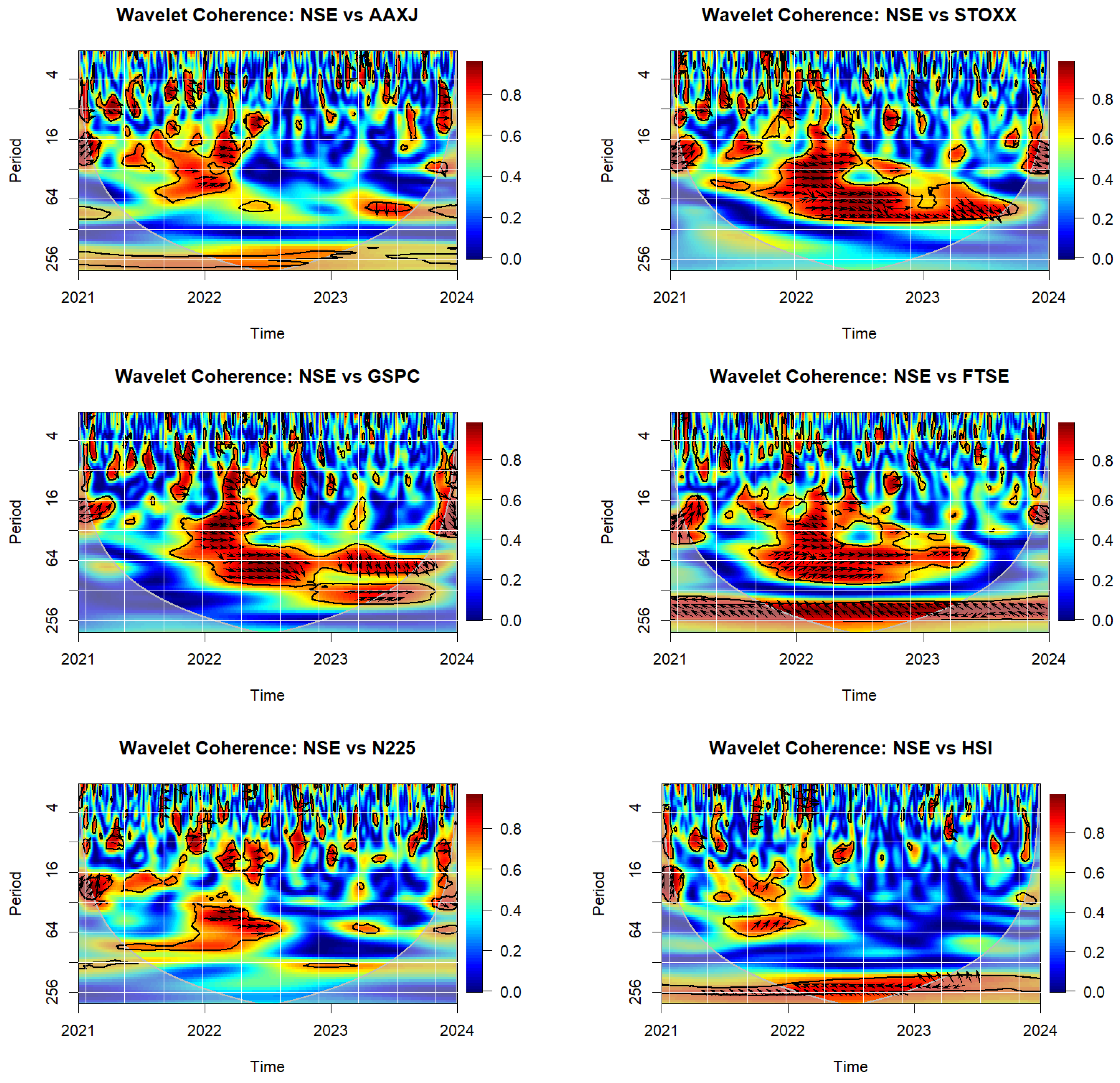
4.5. Wavelet Coherence

The wavelet coherence graph visually depicts the time-varying correlation between two time series data across different frequencies, showing how their relationship changes over time. The wavelet coherence graph is superior for analysing time-varying relationships between two time series across both time and frequency domains. Unlike traditional correlation measures, it reveals how the strength and nature of the relationship evolve over time at different frequencies, making it particularly effective for identifying non-stationary or cyclical patterns. By identifying periods of high coherence between different markets, investors and portfolio managers can recognise when diversification benefits diminish, prompting a shift towards less correlated assets to mitigate risk. Considering the wavelet coherence graph presenting strong long-term synchronisation between market A and B during a particular period, it may be suggested to reduce exposure to market B assets by increasing investments in regions or asset classes exhibiting lower coherence with market A. Conversely, during periods of low or fragmented coherence, the investor may diversify across multiple markets to exploit independent growth trajectories.

The X-axis in the graph represents time, and the Y-axis shows frequency, with short-term interactions at the bottom and long-term at the top. Colour-coded regions illustrate the coherence strength (0 to 1), where red or yellow areas indicate high coherence, indicating strong correlation, and blue signifies low coherence. Arrows in the graph provide additional insights into the phase relationship. Rightward arrows show the series are in-phase, leftward indicate out-of-phase, while upward and downward arrows suggest one series leads the other. The cone of influence outlines the area where interpretations are most reliable, focusing attention within its bounds. The wavelet coherence graph helps identify periods of high or low correlation and any lead–lag relationships, revealing dynamic connections between two time series. Figure 8 shows the wavelet coherence between the Indian stock market and the other global indices, shedding light on the strength and dynamics of their interdependencies across different periods and frequencies.

Generally, there are noticeable periods of high coherence (marked in red) between India and other markets, particularly in the medium- (16–64) to long-term (64–256) periods, suggesting that external shocks have a significant and sustained impact on the Indian market. This is evident, especially during 2022 and 2023, where high coherence regions frequently appear across these indices, indicating that global market trends considerably influenced the Indian market in the aftermath of the COVID-19 pandemic. For instance, the coherence between India and the Global, Emerging Markets, and USA indices shows robust synchronisation, reflecting the effect of heightened economic interconnectivity and the global response to market disruptions caused by the pandemic and subsequent recovery phases.

Another notable observation is that the Indian market’s coherence with European, UK, and Asia Pacific indices reveals a pattern of fluctuating correlation over time, with some high-coherence areas appearing intermittently in short-term periods (4–16), particularly in the latter part of 2023. This could suggest that regional-specific events, such as inflation concerns, policy changes, and geopolitical tensions, also play a role in these correlations, influencing investor behaviour and market responses. Additionally, the Indian market shows varying responses to short-term shocks, as evidenced by the scattered low-coherence (blue) regions. These results indicate that India’s stock market demonstrates a degree of resilience but remains exposed to global volatility, especially during significant economic events. This interconnectedness, highlighted by the wavelet coherence across multiple regions, emphasises the need for investors and policymakers in India to account for both global and regional market conditions in their decision-making processes.

5. Implications

The implications of this study are far-reaching for investors, policymakers, and market regulators, offering crucial insights into the dynamics of global financial market interconnectedness. The results indicate that the Indian stock market exhibits a high sensitivity to shocks from major international indices, particularly during periods of economic turmoil such as the post-pandemic recovery. This information is valuable for investors seeking to optimise portfolio strategies by accounting for the volatility spillover effects from key global markets like the U.S., Europe, and Asia, thereby improving risk management and enhancing returns. Specifically, for the portfolio managers, it is necessary to identify and categorise rising correlations, increased volatility persistence, or periods of high wavelet coherence for better risk mitigation strategies. During periods of heightened market interconnectedness, they may reduce exposure to highly correlated assets or diversify into less volatile regions to safeguard returns. This adaptive strategy, guided by the wavelet-based insights, allows decision-makers to dynamically rebalance portfolios, optimise returns, and strengthen resilience against market shocks by aligning asset allocation with evolving market interdependencies.

For policymakers, the findings highlight the need for proactive measures to bolster market resilience against external shocks, such as creating stronger financial infrastructure, improving regulatory frameworks, and fostering greater economic integration. Additionally, we suggest implication of policies fostering regional cooperation and information-sharing among emerging economies can help mitigate contagion risks by addressing cross-border volatility spillovers. Establishing capital buffer requirements that fluctuate based on wavelet-identified periods of heightened coherence with global markets could pre-empt market disruptions. Moreover, promoting financial literacy and encouraging institutional investors to diversify into asset classes less sensitive to global shocks can reduce overall market fragility. Moreover, the study underscores the importance of dynamic, real-time monitoring of market correlations and volatility, enabling timely policy interventions and more informed decision-making by investors and regulators. Identifying time-varying relationships between markets also stresses the necessity for adaptive strategies that respond to market fluctuations across different frequencies, ensuring that the Indian market remains resilient and competitive in a highly interconnected global economy.

6. Conclusions

This study comprehensively analyses the interconnectedness between the Indian stock market (NSE) and several key global financial indices, using advanced econometric techniques such as the Diebold–Yilmaz spillover index, DCC-GARCH model, and wavelet coherence analysis. The findings reveal significant spillover effects, especially from markets in the U.S., Europe, and Asia, indicating that global events have a lasting impact on the Indian market. The results highlight the need for enhanced risk management strategies and adaptive policy measures, as the Indian market is highly responsive to external shocks, particularly during economic uncertainty. The research also demonstrates the effectiveness of time-varying methods in capturing the dynamic nature of market interdependencies, offering valuable insights for investors, regulators, and policymakers in navigating the complexities of a globally interconnected financial landscape.

7. Limitation and Scope

This study primarily focuses on the volatility spillovers and interdependencies between financial indices, offering critical insights into market dynamics. However, it does not explicitly account for broader macroeconomic variables such as fiscal policies, trade dynamics, monetary interventions, or political stability, which can significantly shape market behaviour. While the use of broad market indices is informative, it may mask sectoral and regional variations that could reveal more focussed patterns of volatility transmission. This generalisation limits the ability to draw conclusions about the behaviour of specific industries or geographic segments within the market. Future research can address these limitations by integrating sector-specific indices, macroeconomic indicators (e.g., inflation rates, interest rates, and government debt levels), and geopolitical risks to develop a more comprehensive understanding of market interdependencies. Expanding the dataset to include indices from economic blocs such as BRICS+, G7, and G20 could yield insights into cross-regional volatility spillovers and diversification opportunities. Additionally, employing alternative econometric models like BEKK-GARCH, TVP-VAR, or machine learning techniques can enhance the accuracy and robustness of the analysis of time-varying correlations. A more focused exploration of causal relationships between markets during critical economic events, such as financial crises, geopolitical conflicts, and pandemics, may uncover underlying drivers of market resilience or fragility. Future studies could also investigate the role of emerging markets in mitigating global risks, shedding light on their evolving influence in fostering financial stability and reducing systemic vulnerabilities across interconnected economies.