Simulation Framework to Determine Suitable Innovations for Volatility Persistence Estimation: The GARCH Approach

Abstract

This study rolls out a robust framework relevant for simulation studies through the Generalised Autoregressive Conditional Heteroscedasticity (GARCH) model using the rugarch package. The package is thoroughly investigated, and novel findings are identified for improved and effective simulations. The focus of the study is to provide necessary simulation steps to determine appropriate distributions of innovations relevant for estimating the persistence of volatility. The simulation steps involve “background (optional), defining the aim, research questions, method of implementation, and summarised conclusion”. The method of implementation is a workflow that includes writing the code, setting the seed, setting the true parameters a priori, data generation process and performance assessment through meta-statistics. These novel, easy-to-understand steps are demonstrated on financial returns using illustrative Monte Carlo simulation with empirical verification. Among the findings, the study shows that regardless of the arrangement of the seed values, the efficiency and consistency of an estimator generally remain the same as the sample size increases. The study also derived a new and flexible true-parameter-recovery measure which can be used by researchers to determine the level of recovery of the true parameter by the MCS estimator. It is anticipated that the outcomes of this study will be broadly applicable in finance, with intuitive appeal in other areas, for volatility modelling.

1. Introduction

A simulation-based experiment is not often included in research because many upcoming researchers do not have an adequate understanding of the nitty-gritty involved. Although the details involved in simulation modelling are generally inexhaustible, this study, however, unveils a crucial framework relevant for the simulation of financial time series data using the Generalised Autoregressive Conditional Heteroscedasticity (GARCH) model for volatility persistence estimation. Volatility persistence describes the effect of a shock to future expectation of the variance process (see Ding and Granger 1996). The ultimate goal of the study is to familiarise researchers with the concepts of simulation modelling through this model. The framework utilises the robust simulating resources of the GARCH model, through set parameters, to generate data that are analysed, and the estimates from the process are then used by chosen metrics to explain the behaviour of selected statistics of interest.

Monte Carlo simulation (MCS) studies are computer-based experiments that use known probability distributions to create data by pseudo-random sampling. The data may be simulated through a parametric model or via repeated resampling (Morris et al. 2019). MCS applies the concept of imitating a real-life scenario on the computer through a certain model that can hypothetically generate the scenario. By simulating or repeating this process a considerably large number of times, it is possible to obtain outcomes that can enable precise computation of desired issues of concern, such as the possible assumed error distribution/s that can suitably describe a given stock market. In preparing for a simulation experiment, reasonably ample time is needed to organise a well-written and readable computer code and for simulated data generation. Implementation of a good simulation experiment and reporting the outcomes require adequate planning.

Series of R application software packages such as the rugarch (Ghalanos 2022), GAS (Ardia et al. 2019), GRETL (Baiocchi and Distaso 2003), fGARCH (Wuertz et al. 2020), SimDesign (Chalmers and Adkins 2020), tidyverse (Wickham et al. 2019), to mention but a few, are currently available for simulation studies. This study exemplifies how the GARCH model through the rugarch package can be effectively used to improve volatility modelling through a MCS experiment, with outcomes verified empirically. The simulation steps are designed to be reasonably general with the expectation that any other related packages1 should be able to replicate the routine. Although there are good books on simulation approaches in general (see Bratley et al. 2011; Kleijnen 2015), up until now, to the best of our knowledge, there has not been any monograph with a direct step-by-step comprehensive layout on a simulation framework using the GARCH model. Hence, this study rolls out an inclusive simulation design that is summarily required for a robust simulation practice in finance to determine appropriate assumed innovations, relevant for estimating the persistence of volatility using this model, with the knowledge applicable in other fields. Here, the MCS approach is used to obtain the most suitable assumed innovation, through which the volatility persistence is empirically estimated.

Since the rugarch package does not make provision for calculating the coverage probability2, this study also computes the MCS estimator’s recovery levels through the “true parameter recovery (TPR)” measure as a proxy for the coverage. The results show that the MCS estimates considerably recover the true parameters. The raw data used for this study are the daily closing S&P South African sovereign bond index, abbreviated to S&P SA bond index. They are Standard & Poor data for the bond market in US dollars from Datastream (2021) for the period 4 January 2000 to 17 June 2021 with 5598 observations. The rest of the paper is organised as follows: Section 2 reviews the theories underpinning two heteroscedastic models, the TPR measure, and the description of the design of the simulation framework. Section 3 presents the practical illustration of the simulation framework, with empirical verification, on financial bond return data. Section 4 discusses the key findings and Section 5 concludes.

2. Materials and Methods

2.1. The GARCH Model

The GARCH model was developed by Bollerslev (1986) as a generalisation of the Autoregressive Conditional Heteroscedasticity (ARCH) model introduced by Engle (1982). It is a classical model that is normally defined by its conditional mean and variance equations for modelling financial returns volatility (Kim et al. 2020). The mean equation is stated as

$$r_t={\mu }_t+{\epsilon }_t,$$

(1)

where $r_t$ is the return series, ${\epsilon }_t=z_t{\sigma }_t$ denotes the residual part of the return series that is random and unpredictable, where $z_t\sim N(0,1)$ are the standardised residuals which are independent and identically distributed (i.i.d.) random variables with mean 0 and variance 1 (McNeil and Frey 2000; Smith 2003), ${\mu }_t$ is the mean function that is usually stated as an Autoregressive Moving Average (ARMA) process,

$${\mu }_t=\sum _{i=1}^p{\varphi }_i{r}_{t-i}+\sum _{i=1}^q{\theta }_i{\epsilon }_{t-i},$$

(2)

where ${\varphi }_i$ (i = 1, …, p) and ${\theta }_i$ (i = 1, …, q) are unknown parameters. The variance equation of the GARCH$(u,v)$ model is defined as

$${\sigma }_t^2=\omega +{\alpha }_1{\epsilon }_{t-1}^2+\cdots +{\alpha }_v{\epsilon }_{t-v}^2+{\beta }_1{\sigma }_{t-1}^2+\cdots +{\beta }_u{\sigma }_{t-u}^2,$$

(3)

where $\omega >0$ is the intercept (white noise), coefficients ${\alpha }_j\ge 0$ (j = 1, …, v) and ${\beta }_i\ge 0$ (i = 1, …, u), respectively, measure the short-term and long-term effects of ${\epsilon }_t$ on the conditional variance (Maciel and Ballini 2017). The non-negativity restrictions on the unknown parameters, ${\alpha }_j$ and ${\beta }_i$, are imposed for ${\sigma }_t^2>0$. The equation shows that the conditional variance ${\sigma }_t^2$ is a linear function of past squared innovation ${\epsilon }_{t-j}^2$ and past conditional variances ${\sigma }_{t-i}^2$. The GARCH model is a more parsimonious specification (Nelson 1991; Samiev 2012) since it is an equivalence of a certain ARCH(∞) model (Zivot 2009). When $u=0$ in Equation (3), the GARCH model changes to the ARCH model with conditional variance stated as

$${\sigma }_t^2=\omega +{\alpha }_1{\epsilon }_{t-1}^2+\cdots +{\alpha }_v{\epsilon }_{t-v}^2.$$

(4)

GARCH(1,1) is the simplest model specification with u = 1 and v = 1 in Equation (3), and it is conceivably the best candidate GARCH model for several applications (Fan et al. 2014; Zivot 2009). The volatility persistence of the GARCH$(1,1)$ model is defined as ${\alpha }_1$ + ${\beta }_1$ (see Engle and Bollerslev 1986; Ghalanos 2018). Volatility persistence is used to evaluate the speed of decay of shocks to volatility (Kim et al. 2020). Volatility exhibits long persistence into the future if $\alpha$ + $\beta$→ 1, hence the closer the sum of the coefficients is to one (zero), the greater (lesser) the persistence. However, if the sum is equal to one, then shocks to volatility persist forever and the unconditional variance is not determined by the model. This process is called integrated-GARCH (Chou 1988; Engle and Bollerslev 1986). If the sum is greater than one, the conditional variance process is explosive, suggesting that shocks to the conditional variance are highly persistent. Covariance stationarity of the GARCH model is ensured when ${\sum }_{j=1}^v{\alpha }_j+{\sum }_{i=1}^u{\beta }_i<1$, while the unconditional variance of ${\epsilon }_t$ is ${\sigma }^2=E\left({\epsilon }_t^2\right)=\omega /\{1-({\sum }_{j=1}^v{\alpha }_j+{\sum }_{i=1}^u{\beta }_i)\}$ (Zivot 2009).

For the maximum likelihood estimation (MLE), the log-likelihood function for maximising the likelihood of the unknown parameters given the observations is stated as

$$L\left(\vartheta \right|\epsilon )=\sum _{t=1}^N\frac{1}{\sqrt{2\pi {\sigma }_t^2}}\exp \left(-\frac{{\epsilon }_t^2}{2{\sigma }_t^2}\right),$$

(5)

where $\vartheta ={(\mu ,\omega ,{\alpha }_1,\dots ,{\alpha }_v,{\beta }_1,\dots ,{\beta }_u)}^{\top }$ is a vector of parameters, and $\epsilon =({\epsilon }_1,\dots ,{\epsilon }_N)$ is a realisation of length N. The quasi-maximum likelihood estimation (QMLE) based on the Normal distribution and MLE have the same set of instructions for estimating $\widehat{\vartheta }$; the only difference, however, is in the estimation of a robust standard deviation of $\widehat{\vartheta }$ (see Bollerslev and Wooldridge 1992; Feng and Shi 2017; Francq and Zakoïan 2004).

The maximised log-likelihood function with Student’s t distribution (Duda and Schmidt 2009) is stated as

$$lnL\left(\vartheta \right|\epsilon )=\sum _{t=1}^N\left(ln\left[\frac{\Gamma \left(\frac{\nu +1}{2}\right)}{\Gamma \left(\frac{\nu }{2}\right)\sqrt{(\nu -2)\pi }}\right]-\frac{1}{2}ln\left({\sigma }^2\right)-\left(\frac{\nu +1}{2}\right)ln\left[1+\frac{{\epsilon }_t^2}{{\sigma }^2(\nu -2)}\right]\right),$$

(6)

where $\Gamma (·)$ and $\nu$ are the gamma function and degree of freedom, respectively.

2.2. The fGARCH Model

The family GARCH (fGARCH) model, developed by Hentschel (1995), is an inclusive model that nests some important symmetric and asymmetric GARCH models as sub-models. The nesting includes the simple GARCH (sGARCH) model (Bollerslev 1986), the Absolute Value GARCH (AVGARCH) model (Schwert 1990; Taylor 1986), the GJR GARCH (GJRGARCH) model (Glosten et al. 1993), the Threshold GARCH (TGARCH) model (Zakoian 1994), the Nonlinear ARCH (NGARCH) model (Higgins and Bera 1992), the Nonlinear Asymmetric GARCH (NAGARCH) model (Engle and Ng 1993), the Exponential GARCH (EGARCH) model (Nelson 1991), and the Asymmetric Power ARCH (apARCH) model (Ding et al. 1993). The sub-model apARCH is also a family model (but less general than the fGARCH model) that nests the sGARCH, AVGARCH, GJRGARCH, TGARCH, NGARCH models, and the Log ARCH model (Geweke 1986; Pantula 1986). The fGARCH$(u,v)$ model is stated as

$${\sigma }_t^{\gamma }=\omega +\sum _{j=1}^v{\alpha }_j{\sigma }_{t-j}^{\gamma }\left(\right|z_{t-j}-{\lambda }_{2j}{|-{\lambda }_{1j}\{z_{t-j}-{\lambda }_{2j}\})}^{\delta }+\sum _{j=1}^u{\beta }_j{\sigma }_{t-j}^{\gamma }.$$

(7)

This robust fGARCH model allows different powers for ${\sigma }_t$ and $z_t$ to drive how the residuals are decomposed in the conditional variance equation. Equation (7) is the conditional standard deviation’s Box–Cox transformation, where the transformation of the absolute value function is carried out by the parameter $\delta$, and $\gamma$ determines the shape. The ${\lambda }_{2j}$ and ${\lambda }_{1j}$ control the shifts for asymmetric small shocks and rotations for large shocks, respectively. The fit of the full fGARCH model can be implemented with $\gamma$ = $\delta$ (see Ghalanos 2018). Volatility clustering in the returns can be quantified through the model’s volatility persistence stated as

$$\widehat{P}=\sum _{j=1}^u{\beta }_j+\sum _{j=1}^v{\alpha }_j{\varrho }_j,$$

(8)

where ${\varrho }_j$, expressed in Equation (9), is the expected value of $z_t$ in the absolute value asymmetry term’s Box–Cox transformation. Volatility clustering implies that large changes in returns tend to be followed by large changes and small changes tend to be followed by small changes. The persistence is obtained in this study through the “persistence()” function in the R rugarch package. See (Ghalanos 2022; Hentschel 1995) for details on fGARCH and the nested models.

$${\displaystyle {\varrho }_j=\mathtt{E}(|z_{t-j}-{\lambda }_{2j}|-{\lambda }_{1j}(z_{t-j}-{\lambda }_{2j}){)}^{\delta }={\int }_{-\infty }^{\infty }\left(\right|z-{\lambda }_{2j}{|-{\lambda }_{1j}(z-{\lambda }_{2j}))}^{\delta }f(z,0,1,\dots )dz}$$

(9)

2.3. The True Parameter Recovery Measure

Since the focus of MCS studies involves the ability of the estimator to recover the true parameter (see Chalmers 2019), this study applies the “true parameter recovery (TPR)” measure in Equation (10) to compute the level (degree) of recovery of the true parameter through the MCS estimator. The TPR measure is a means of evaluating the performance of the MCS estimates in recovering the true parameter. That is, it is used to determine how much of the true parameter value is recovered by the MCS estimator.

$$\mathrm{TPR}=\left(K-\left[\frac{(\vartheta -\widehat{\vartheta })}{\vartheta }\times K\right]\right)\%,$$

(10)

where K = 0, 1, 2, …, 100 is the nominal recovery level, $\vartheta$ is the true data-generating parameter and $\widehat{\vartheta }$ is the estimator from the simulated (synthetic) data. For instance, a TPR estimated value of 95% or 100% denotes that the MCS estimator recovers the complete 95% or 100% of the true parameter. This complete recovery of the true parameter $\vartheta$ can be achieved by the MCS estimator $\widehat{\vartheta }$ when $\widehat{\vartheta }$ = $\vartheta$, where $\vartheta >0$, such that the TPR outcome equals the given nominal recovery level K (i.e., TPR = K%).

2.4. Simulation Design

The design of the simulation framework includes “background (optional), defining the aim, research questions, method of implementation, and summarised conclusion”. The method of implementation is a workflow that involves writing the code, setting the seed, setting the true parameter/s a priori, data generation process, and performance evaluation through meta-statistics. As summarised by the flowchart in Figure 1, these crucial steps are relevant for successful simulations through the GARCH model. The details of each design step are as follows:

2.4.1. Aim of the Simulation Study

After optionally stating the background that explains crucial underlying facts about the study, the next step is to define the aim of the study, and it must be clearly, concisely and unambiguously stated for the reader’s understanding. The focus of MCS studies generally dwells on estimators’ capabilities in recovering the true parameters $\vartheta$, such that E$\left(\widehat{\vartheta }\right)$ = $\vartheta$ for unbiasedness, $\widehat{\vartheta }\to \vartheta$ as the sample size $N\to \infty$ for consistency, and root mean square error (RMSE) or standard error (SE) tends to zero as $N\to \infty$ for good efficiency or precision of the true parameter’s estimator. Hence, the aim of the study may revolve around those properties, such as bias or unbiasedness, consistency, efficiency or precision of the estimator. The aim can also evolve from comparisons of multiple entities, such as comparing the efficiency of various error distributions, or comparing the performance of multiple models, or on improvement to an existing method.

2.4.2. State the Research Questions

After defining the study’s aim, relevant questions concerning the purpose of the simulation should be outlined. These will be pointers to the objectives of the study. The intricacies of some statistical research questions make them better resolved via simulation approaches. Simulation provides a robust procedure for responding to a wide range of theoretical and methodological questions and can offer a flexible structure for answering specific questions pertinent to researchers’ quest (Hallgren 2013).

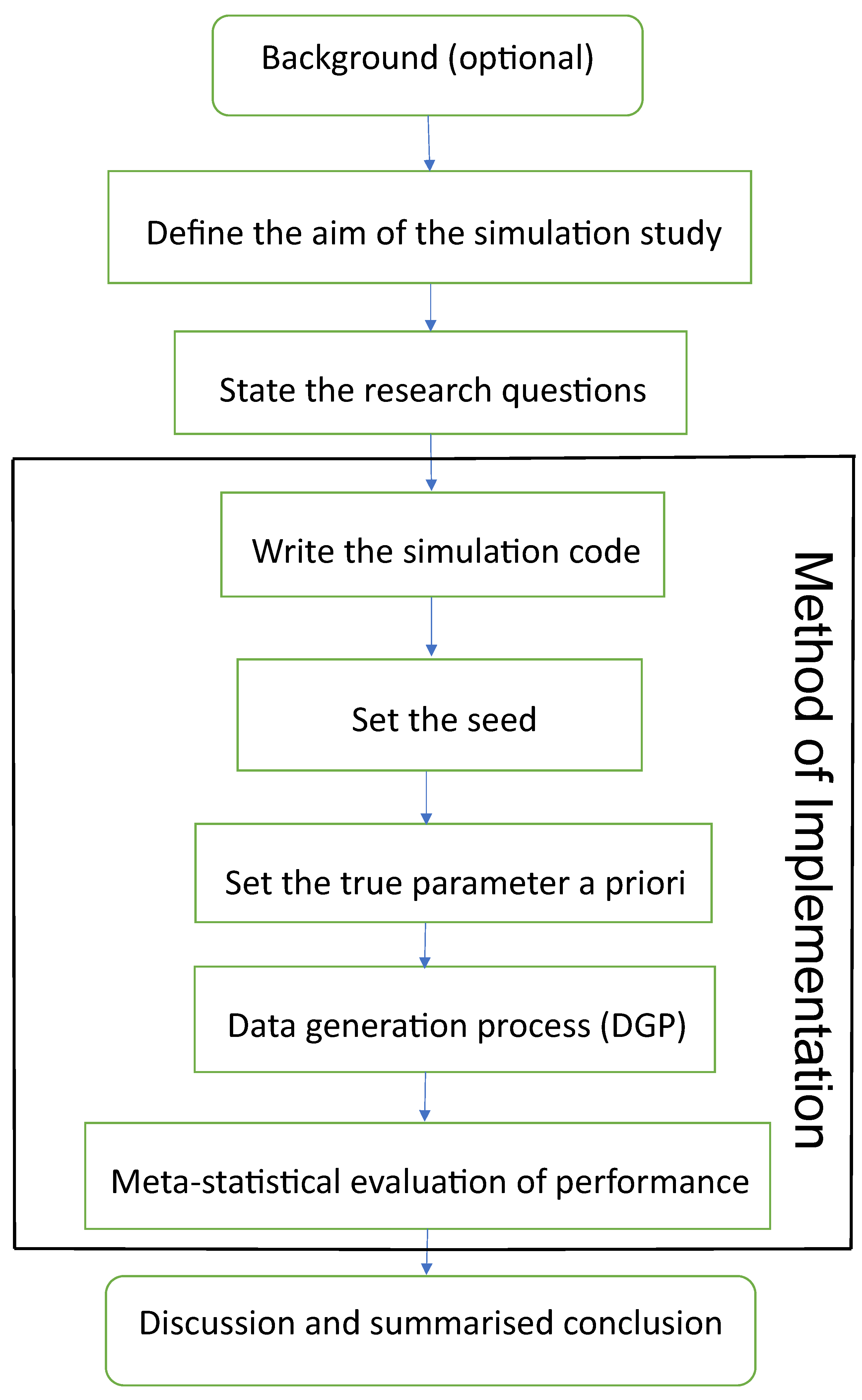
2.4.3. Method of Implementation

The simulation and empirical modelling of this study are implemented in R Statistical Software, version 4.0.3, with RStudio version 2022.12.0+353, using the rugarch (Ghalanos 2018, 2022), SimDesign (Chalmers and Adkins 2020), tidyverse (Wickham et al. 2019), zoo (Zeileis and Grothendieck 2005), aTSA (Qiu 2015) and forecast (Hyndman and Khandakar 2008) packages. Computation is executed on Intel(R) Core(TM) i5-8265U CPU @ 1.60GHz 1.80 GHz. The method of implementing the simulation is as follows:

• Write the code: Carrying out a proper simulation experiment that mirrors real-life situations can be very demanding and computationally intensive, hence readable computer code with the right syntax must be produced. The code in this study is written to fit the true model3 to the real data to obtain the true parameter representations4 for the MCS. These true parameter values and other outputs from the fit are used in the code to generate simulated datasets that are analysed to obtain the MCS estimators. The standard errors of the estimates are also obtained in the process.
• Set the seed: Simulation code will generate a different sequence of random numbers each time it is run unless a seed is set (Danielsson 2011). A set seed initialises the random number generator (Ghalanos 2022) and ensures reproducibility, where the same result is obtained for different runs of the simulation process (Foote 2018). The seed needs to be set only once, for each simulation, at the start of the simulation session (Ghalanos 2022; Morris et al. 2019), and it is better to use the same seed values throughout the process (Morris et al. 2019).

Now, through the GARCH model, this study carries out an MCS experiment to ascertain whether the seed values’ pattern or arrangement affects the estimators’ efficiency and consistency properties. Two sets of seeds are used for the experiment, where each set contains three different patterns of seed values. The first set is $S_1$ = {12345, 54321, 15243}, while the second set $S_2$ = {34567, 76543, 36547}. In each set, the study tries to use seed values arranged in ascending order, then reverses the order, and finally mixes up the ordered arrangement. The simulation starts by using GARCH(1,1)-Student’s t, with a degree of freedom $\nu$ = 3, as the true model under four assumed error distributions of a Normal, Student’s t, Generalised Error Distribution (GED) and Generalised Hyperbolic (GHYP) distribution. Details on these selected error distributions can be seen in Ghalanos (2018) and Barndorff-Nielsen et al. (2013). The true parameter values used are ($\mu$, $\omega$, $\alpha$, $\beta$) = (0.0678, 0.0867, 0.0931, 0.9059), and they are obtained by fitting GARCH(1,1)-Student’s t to the SA bond return data.

Using each of the seed patterns in turn, simulated datasets of sample size N = 12,000, repeated 1000 times are generated through the parameter values. However, because of the effect of initial values in the data generating process, which may lead to size distortion (Su 2011), the first N = {11,000, 10,000, 9000, 8000} sets of observations are each discarded at each stage of the generated 12,000 observations to circumvent such distortion. That is, only the last N = {1000, 2000, 3000, 4000} are used under each of the four assumed error distributions, as shown in

Table A1. Outcomes of different patterns of seed values, with true parameter $\alpha +\beta$ = 0.9990.

$\mathbf{Panel}\mathbf{A}$ (${\mathit{S}}_1$)		Seed: 12345				Seed: 54321				Seed: 15243
	$\mathit{N}$	$\widehat{\mathit{\alpha }}+\widehat{\mathit{\beta }}$	RMSE${}_{\widehat{\mathit{\alpha }}+\widehat{\mathit{\beta }}}$	SE${}_{\widehat{\mathit{\alpha }}+\widehat{\mathit{\beta }}}$	TPR (95%)	$\widehat{\mathit{\alpha }}+\widehat{\mathit{\beta }}$	RMSE${}_{\widehat{\mathit{\alpha }}+\widehat{\mathit{\beta }}}$	SE${}_{\widehat{\mathit{\alpha }}+\widehat{\mathit{\beta }}}$	TPR (95%)	$\widehat{\mathit{\alpha }}+\widehat{\mathit{\beta }}$	RMSE${}_{\widehat{\mathit{\alpha }}+\widehat{\mathit{\beta }}}$	SE${}_{\widehat{\mathit{\alpha }}+\widehat{\mathit{\beta }}}$	TPR (95%)
Normal	1000	0.9990	0.0862	0.0862	95.00%	0.9563	0.0757	0.0625	90.94%	0.9909	0.0801	0.0796	94.23%
	2000	0.9771	0.0934	0.0908	92.91%	0.9903	0.0419	0.0410	94.17%	0.9839	0.0490	0.0466	93.56%
	3000	0.9727	0.0756	0.0709	92.50%	0.9850	0.0373	0.0345	93.67%	0.9791	0.0591	0.0557	93.11%
	4000	0.9700	0.0693	0.0629	92.24%	0.9846	0.0412	0.0387	93.64%	0.9972	0.0304	0.0303	94.83%
Student’s t	1000	0.9990	0.0525	0.0525	95.00%	0.9833	0.0441	0.0412	93.50%	0.9990	0.0768	0.0768	95.00%
	2000	0.9902	0.0500	0.0492	94.16%	0.9990	0.0349	0.0349	95.00%	0.9958	0.0388	0.0386	94.69%
	3000	0.9973	0.0327	0.0327	94.83%	0.9977	0.0308	0.0308	94.87%	0.9956	0.0318	0.0316	94.68%
	4000	0.9918	0.0277	0.0267	94.31%	0.9974	0.0258	0.0258	94.85%	0.9963	0.0247	0.0246	94.74%
GED	1000	0.9875	0.0719	0.0710	93.90%	0.9688	0.0499	0.0397	92.13%	0.9899	0.0630	0.0624	94.13%
	2000	0.9663	0.0608	0.0512	91.89%	0.9908	0.0336	0.0326	94.22%	0.9847	0.0387	0.0360	93.64%
	3000	0.9684	0.0441	0.0317	92.09%	0.9846	0.0347	0.0315	93.63%	0.9795	0.0385	0.0333	93.15%
	4000	0.9692	0.0410	0.0282	92.16%	0.9833	0.0328	0.0288	93.51%	0.9839	0.0300	0.0259	93.57%
GHYP	1000	0.9940	0.0557	0.0555	94.52%	0.9785	0.0437	0.0386	93.05%	0.9897	0.0657	0.0650	94.12%
	2000	0.9748	0.0507	0.0446	92.70%	0.9979	0.0328	0.0328	94.89%	0.9871	0.0364	0.0344	93.87%
	3000	0.9780	0.0353	0.0284	93.00%	0.9901	0.0305	0.0292	94.15%	0.9849	0.0325	0.0293	93.66%
	4000	0.9776	0.0322	0.0241	92.97%	0.9898	0.0263	0.0247	94.12%	0.9892	0.0247	0.0226	94.07%
$\mathbf{Panel}\mathbf{B}$ ($S_2$)		Seed: 34567				Seed: 76543				Seed: 36547
	$\mathit{N}$	$\widehat{\mathit{\alpha }}+\widehat{\mathit{\beta }}$	RMSE${}_{\widehat{\mathit{\alpha }}+\widehat{\mathit{\beta }}}$	SE${}_{\widehat{\mathit{\alpha }}+\widehat{\mathit{\beta }}}$	TPR (95%)	$\widehat{\mathit{\alpha }}+\widehat{\mathit{\beta }}$	RMSE${}_{\widehat{\mathit{\alpha }}+\widehat{\mathit{\beta }}}$	SE${}_{\widehat{\mathit{\alpha }}+\widehat{\mathit{\beta }}}$	TPR (95%)	$\widehat{\mathit{\alpha }}+\widehat{\mathit{\beta }}$	RMSE${}_{\widehat{\mathit{\alpha }}+\widehat{\mathit{\beta }}}$	SE${}_{\widehat{\mathit{\alpha }}+\widehat{\mathit{\beta }}}$	TPR (95%)
Normal	1000	0.9856	0.0583	0.0568	93.72%	0.9942	0.0424	0.0421	94.54%	0.9823	0.3888	0.3884	93.41%
	2000	0.9814	0.0396	0.0354	93.33%	0.9891	0.0370	0.0357	94.06%	0.9806	0.1419	0.1407	93.25%
	3000	0.9845	0.0708	0.0693	93.62%	0.9809	0.0334	0.0281	93.28%	0.9822	0.0805	0.0787	93.40%
	4000	0.9990	0.0397	0.0397	95.00%	0.9778	0.0326	0.0248	92.98%	0.9779	0.0575	0.0535	92.99%
Student’s t	1000	0.9971	0.0474	0.0474	94.82%	0.9990	0.0422	0.0422	95.00%	0.9990	0.0329	0.0329	95.00%
	2000	0.9789	0.0364	0.0303	93.08%	0.9990	0.0281	0.0281	95.00%	0.9990	0.0315	0.0315	95.00%
	3000	0.9781	0.0326	0.0249	93.01%	0.9975	0.0237	0.0236	94.86%	0.9990	0.0234	0.0234	95.00%
	4000	0.9871	0.0253	0.0223	93.87%	0.9955	0.0218	0.0215	94.67%	0.9946	0.0238	0.0234	94.58%
GED	1000	0.9802	0.0463	0.0423	93.21%	0.9899	0.0389	0.0378	94.13%	0.9986	0.0490	0.0490	94.96%
	2000	0.9726	0.0386	0.0282	92.49%	0.9898	0.0280	0.0265	94.13%	0.9879	0.0388	0.0371	93.94%
	3000	0.9710	0.0398	0.0282	92.33%	0.9820	0.0276	0.0218	93.38%	0.9808	0.0303	0.0243	93.27%
	4000	0.9800	0.0285	0.0213	93.19%	0.9782	0.0284	0.0194	93.02%	0.9752	0.0321	0.0215	92.73%
GHYP	1000	0.9863	0.0436	0.0417	93.80%	0.9928	0.0383	0.0378	94.41%	0.9990	0.0370	0.0370	95.00%
	2000	0.9744	0.0377	0.0285	92.66%	0.9952	0.0265	0.0262	94.64%	0.9990	0.0358	0.0358	95.00%
	3000	0.9737	0.0351	0.0242	92.59%	0.9872	0.0243	0.0213	93.88%	0.9894	0.0256	0.0237	94.09%
	4000	0.9810	0.0278	0.0212	93.29%	0.9835	0.0246	0.0192	93.53%	0.9816	0.0275	0.0213	93.35%

, Appendix A. These trimming steps are carried out following the simulation structure of Feng and Shi (2017)5. An observation-driven process such as the GARCH can be size-distorted with regards to its kurtosis, where strong size distortion may be a result of high kurtosis (Silvennoinen and Teräsvirta 2016). The extracts of the RMSE and SE outcomes for the GARCH volatility persistence estimator $\widehat{\alpha }+\widehat{\beta }$ are shown in Table A1. For $S_1$ in Panel A of the table, as N tends to its peak, the performance of the RMSE from the lowest to the highest under the four error distribution assumptions is Student’s t, GHYP, GED and Normal in that order, while that of SE from the lowest to the highest is GHYP, Student’s t, GED and Normal in that order, for the three arrangements of seed values.

For $S_2$ in Panel B of the table, as N reaches its peak at 4000, the performance of the RMSE from the lowest to the highest is Student’s t, GHYP, GED and Normal in that order, while that of SE from the lowest to the highest is GHYP, GED, Student’s t and Normal in that order, for the three $S_2$ patterns of seed values. Hence, efficiency and precision in terms of RMSE and SE are the same as the sample size N becomes larger under the three seeds, regardless of the arrangement of the seed values under $S_2$, as also observed under $S_1$. In addition, the flows of $\sqrt{N}$ consistency of the estimator under the seed values in $S_1$ are roughly the same; this is also applicable to those of the seed values in $S_2$. The plotted outcomes can be visualised as displayed by the trend lines within the 95% confidence intervals in Figure 2 for the three seed values of sets $S_1$ in Panel A and $S_2$ in Panel B, where the efficiency and consistency outcomes are roughly the same with increase in N.

To summarise, this study observes that, as $N\to \infty$, the pattern or arrangement of the seed values does not affect the estimator’s overall consistency and efficiency properties, but this may likely depend on the quality of the model used. The seed is primarily used to ensure reproducibility. Panels C and D of the figure further reveal that the RMSE/SE → 0 as $N\to \infty$ for the four error distributions in $S_1$ and $S_2$.

Table A1 further shows that the MCS estimator $\widehat{\alpha }+\widehat{\beta }$ considerably recovers the true parameter $\alpha +\beta$ at the 95% nominal recovery level, where some of the estimates even recover the complete true value (0.9990) with TPR outcomes of 95%. These recovery outcomes can be seen in the visual plots of Figure 3 (or as shown in Panels A and B of Figure A1, Appendix B), where Panels A(i) and B(i) reveal that the MCS estimates perform quite well in recovering the true parameter as shown by the closeness of the TPR outcomes to the 95% (i.e., 0.95) nominal recovery level for $S_1$ and $S_2$, respectively. The bunched up TPR outcomes in Panels A(i) and B(i) are clearly spread out as shown in Panels A(ii) and B(ii) for $S_1$ and $S_2$, respectively. From these recovery outputs, two distinct features can be observed. First, the TPR results do not depend on the sample size as shown in Panels A and B of Figure 4 for $S_1$ and $S_2$, which is a feature of coverage probability (see Hilary 2002); second, the closer (farther) the MCS estimate is to zero, the smaller (larger) the TPR outcome, as revealed in Panels C and D of the figure.

• After setting the seed, the true parameter representations of the true sampling distribution (or true model) are then set a priori (Koopman et al. 2017; Mooney 1997).
• Next, simulated observations are generated using the true sampling distribution or the true model given some sets of (or different sets of) fixed parameters. Generation of simulated datasets through the GARCH model is carried out using the R package “rugarch”. Random data generation involving this package can be implemented using either of two approaches. The first approach is to carry out the data-generating simulation directly on a fitted object “fit” using the ugarchsim function for the simulated random data. The second approach uses the ugarchpath function, which enables simulation of desired number of volatility paths through different parameter combinations (see Ghalanos 2018, 2022; Pfaff 2016 for relevant details on the two functions and their usage).

The simulation or data-generating process can be run once or replicated multiple times. This study carries out another MCS investigation through the GARCH model to determine the effect (on the outcomes) of running a given GARCH simulation once or replicating it multiple times. That is, for a given sample size and seed value, the outcome of running the simulation once is compared to that of running it with different replications such as 2500, 1000 and 300. This MCS experiment uses GARCH(1,1)-Student’s t, with $\nu$ = 3, as the true model under four assumed error distributions of a Normal, Student’s t, GED and GHYP. However, it should be understood that any non-normal error distributions (apart from the Student’s t that is used here) can also be used with GARCH(1,1) model for the true model. The GARCH(1,1)-Student’s t fitted to the SA bond return data yields the true parameter values ($\mu$, $\omega$, $\alpha$, $\beta$) = (0.0678, 0.0867, 0.0931, 0.9059).

Using these parameter values, datasets of sample size N = 12,000 are generated in each of the four distinct simulations (i.e., simulations with 1, 2500, 1000 and 300 replicates). After necessary trimmings in each simulation, to evade initial values effect, the last N = {1000, 2000, 3000} sets of observations are used at each stage of the generated 12,000 observations under the four assumed innovation distributions. That is, datasets of the last three sample sizes, each simulated once, then replicated L = {2500, 1000, and 300} times are consecutively generated. From the modelling outputs, it is observed that the log-likelihood (llk), RMSE, SE and bias outcomes of $\widehat{\alpha }$, $\widehat{\beta }$ and $\widehat{\alpha }+\widehat{\beta }$ estimators for each simulation under the four assumed errors are the same for the three sample-size datasets with the same seed value, regardless of whether the simulation is run once or replicated multiple times. For brevity, this study only displays the outcomes of the experiment under the assumed GED error for each run in

Table 1. Outcomes of different simulation replicates.

Panel A: Simulation run once
$\mathit{\alpha }$	$\mathit{\beta }$	$\mathit{N}$	llk	RMSE${}_{\widehat{\mathit{\alpha }}}$	Bias${}_{\widehat{\mathit{\alpha }}}$	SE${}_{\widehat{\mathit{\alpha }}}$	RMSE${}_{\widehat{\mathit{\beta }}}$	Bias${}_{\widehat{\mathit{\beta }}}$	SE${}_{\widehat{\mathit{\beta }}}$	RMSE${}_{\widehat{\mathit{\alpha }}+\widehat{\mathit{\beta }}}$	Bias${}_{\widehat{\mathit{\alpha }}+\widehat{\mathit{\beta }}}$	SE${}_{\widehat{\mathit{\alpha }}+\widehat{\mathit{\beta }}}$
0.0931	0.9059	1000	−2020.5	0.0504	0.0328	0.0383	0.0551	−0.0443	0.0327	0.0719	−0.0115	0.0710
		2000	−3813.8	0.0246	0.0046	0.0241	0.0462	−0.0374	0.0271	0.0608	−0.0327	0.0512
		3000	−5734.2	0.0156	−0.0037	0.0152	0.0316	−0.0269	0.0166	0.0441	−0.0306	0.0317
Panel B: Simulation run with 2500 replications
0.0931	0.9059	1000	−2020.5	0.0504	0.0328	0.0383	0.0551	−0.0443	0.0327	0.0719	−0.0115	0.0710
		2000	−3813.8	0.0246	0.0046	0.0241	0.0462	−0.0374	0.0271	0.0608	−0.0327	0.0512
		3000	−5734.2	0.0156	−0.0037	0.0152	0.0316	−0.0269	0.0166	0.0441	−0.0306	0.0317
Panel C: Simulation run with 1000 replications
0.0931	0.9059	1000	−2020.5	0.0504	0.0328	0.0383	0.0551	−0.0443	0.0327	0.0719	−0.0115	0.0710
		2000	−3813.8	0.0246	0.0046	0.0241	0.0462	−0.0374	0.0271	0.0608	−0.0327	0.0512
		3000	−5734.2	0.0156	−0.0037	0.0152	0.0316	−0.0269	0.0166	0.0441	−0.0306	0.0317
Panel D: Simulation run with 300 replications
0.0931	0.9059	1000	−2020.5	0.0504	0.0328	0.0383	0.0551	−0.0443	0.0327	0.0719	−0.0115	0.0710
		2000	−3813.8	0.0246	0.0046	0.0241	0.0462	−0.0374	0.0271	0.0608	−0.0327	0.0512
		3000	−5734.2	0.0156	−0.0037	0.0152	0.0316	−0.0269	0.0166	0.0441	−0.0306	0.0317

. However, increasing the number of replications may reduce sampling uncertainty in meta-statistics (Chalmers and Adkins 2020).

• The generated (simulated) data are analysed, and the estimates from them are evaluated using classic methods through meta-statistics to derive relevant information about the estimators. Meta-statistics (see Chalmers and Adkins 2020) are performance measures or metrics for assessing the modelling outputs by judging the closeness between an estimate and the true parameter. A few of the frequently used meta-statistical summaries, as described below, include bias, root mean square error (RMSE) and standard error (SE). For more meta-statistics, see Chalmers and Adkins (2020); Morris et al. (2019); Sigal and Chalmers (2016).

Bias

The bias, on average, measures the tendency of the simulated estimators $\widehat{\vartheta }$ to be smaller or larger than their true parameter value $\vartheta$. It is defined as the average difference between the true (population) parameter and its estimate (Feng and Shi 2017). The optimal value of bias is 0 (Harwell 2018; Sigal and Chalmers 2016). An unbiased estimator, on average, yields the correct value of the true parameter. Bias with a positive (negative) value indicates that the true parameter value is over-estimated (under-estimated). However, in absolute values, the closer the estimator is to 0, the better it is. Bias is stated mathematically as $\mathtt{E}(\tilde{\vartheta }-\vartheta )$, but can be presented in MCS (see Chalmers 2019) as $bias=\frac{1}{L}{\sum }_{i=1}^L(\widehat{{\vartheta }_i}-\vartheta )$. The two formulae are connected as

$$\mathtt{E}(\tilde{\vartheta }-\vartheta )=\mathtt{E}(\tilde{\vartheta })-\vartheta =\frac{1}{L}\sum _{i=1}^L{\widehat{\vartheta }}_i-\vartheta =\frac{1}{L}\sum _{i=1}^L({\widehat{\vartheta }}_i-\vartheta ),$$

(11)

where $\tilde{\vartheta }$ = ${\widehat{\vartheta }}_i(i=1,\dots ,L)$ is a finite ith number of the sample estimate $\widehat{\vartheta }$ for the datasets, L is the number of replications, and $\vartheta$ is the true parameter.

Standard Error

Sampling variability in the estimation can be evaluated via the standard error (SE) as stated (see Chalmers 2019; Yuan et al. 2015) in Equation (12). Also called Monte Carlo standard deviation, it is a measure of the efficiency or precision of the true parameter’s estimator, which is used to estimate the long-run standard deviation of ${\widehat{\vartheta }}_i$ for finite repetitions. It does not require knowing the true parameter $\vartheta$ but depends on its estimator ${\widehat{\vartheta }}_i$ only. The smaller the sampling variability, the more the efficiency or precision of the $\vartheta$’s estimator (see Morris et al. 2019). Sampling variability decreases with increased sample size (Sigal and Chalmers 2016).

$$\mathrm{SE}=\sqrt{\frac{1}{L}{\sum }_{i=1}^L{({\widehat{\vartheta }}_i-\overline{\vartheta })}^2},\mathrm{where}\overline{\vartheta }=\sum _{i=1}^L\widehat{\vartheta }/L.$$

(12)

RMSE

The root mean square error (RMSE) is an accuracy measure for evaluating the difference between a model’s true value and its prediction. RMSE measure indicates the sampling error of an estimator when compared to the true parameter value (Sigal and Chalmers 2016) and it is stated as

$$\mathrm{RMSE}=\sqrt{\frac{1}{L}{\sum }_{i=1}^L{\left({\widehat{\vartheta }}_i-\vartheta \right)}^2}.$$

(13)

Its computation involves the true parameter $\vartheta$. An estimator with lesser RMSE is more efficient in recovering the true parameter value (Sigal and Chalmers 2016; Yuan et al. 2015), and minimum RMSE produces maximum precision (Wang et al. 2018). Consistency of the estimator occurs when RMSE decreases such that $\widehat{\vartheta }\to \vartheta$ as the sample size $N\to \infty$ (Ghalanos 2018; Morris et al. 2019). RMSE is related to bias and sampling variability as

$$\mathrm{RMSE}=\sqrt{{\mathrm{bias}}^2+{\mathrm{SE}}^2}.$$

(14)

That is, the RMSE is an inclusive measure that combines bias and SE, such that low SE can be penalised for bias. The mean squared error (MSE) is obtained by squaring the RMSE. MCS is highly reliant on the law of large numbers, and it is expected that the distribution of an appropriately large sample should converge to that of the underlying population as the sample size increases (Gilli et al. 2019). It is also expected that the Monte Carlo sampling error should decrease as the sample size increases, but this is not always the case. That is, the sample size cannot always be sufficiently increased to limit the sampling error to a tolerable level (Gilli et al. 2019).

2.4.4. Discussion and Summary

After implementing the method, the last stage in the framework steps is the conclusion, which needs to reflect a summary discussion of all logical findings from the experiments, with answers to the research questions. The conclusion brings out the novelty of the research and may also include the limitations experienced and opportunities for future work. In addition, relevant information on simulation results can be conveyed through graphics, tabular presentation, or both.

3. Results: Simulation and Empirical

3.1. Practical Illustrations of the Simulation Design: Application to Bond Return Data

By way of illustration, this section practically describes how the stated steps can be applied using Monte Carlo simulations with a real data empirical verification.

3.1.1. The Background

It is believed that observation-driven models can appropriately estimate volatility when fitted with a suitable error distribution (Bollerslev 1987). Observation-driven modelling exists in the presence of time-varying parameters, where parameters are functions of lagged dependent variables, concurrent variables and lagged exogenous variables (see Buccheri et al. 2021; Creal et al. 2013 for details). Data generation using the rugarch package can be performed through a variety of models that include the simple GARCH, the exponential GARCH (EGARCH), the GJR-GARCH, the Component GARCH (CGARCH) (Lee and Engle 1999), the Multiplicative Component GARCH (MCGARCH) (Engle and Sokalska 2012), among others, and two omnibus models apARCH and fGARCH (as described in Section 2.2).

The apARCH model is less robust than the fGARCH model (Ghalanos 2018), hence the latter is used for the data generation in this study. Specifically, fGARCH(1,1) model is used as the true data-generating process (DGP) for the MC simulation because the first lag of conditional variability can considerably capture volatility clustering existing in the time series data. In other words, the dependence of volatility on recent past activities is more than on distant past activities (Javed and Mantalos 2013). Hence, this illustrative study showcases the effectiveness of the observation-driven model fGARCH for estimating the persistence of volatility, where the outcomes of the model fitted with each of ten assumed innovation distributions of the Normal, skew-Normal, Student’s t, skew-Student’s t, GED, skew-GED, GHYP, Normal Inverse Gaussian (NIG), Generalised Hyperbolic Skew-Student’s t (GHST) distribution and Johnson’s reparametrised SU (JSU) distribution are compared. Details on the error distributions can be found in Ashour and Abdel-hameed (2010); Azzalini (1985); Azzalini and Capitanio (2003); Barndorff-Nielsen et al. (2013); Branco and Dey (2001); Eling (2014); Ghalanos (2018); Lee and Pai (2010); Pourahmadi (2007).

The DGP fGARCH(1,1) model, as stated in Equation (15), is used to generate simulated return observations using the non-Normal Student’s t error with $\nu$ = 4.1 as the true error distribution.

$${\sigma }_t^{\gamma }=\omega +{\alpha }_1{\sigma }_{t-1}^{\gamma }\left(\right|z_{t-1}-{\lambda }_{21}{|-{\lambda }_{11}\{z_{t-1}-{\lambda }_{21}\})}^{\delta }+{\beta }_1{\sigma }_{t-1}^{\gamma }$$

(15)

Here, a Student’s t with shape parameter or degree of freedom $\nu$ = 4.1 is used to ensure that $\mathtt{E}\left[z_t^4\right]$ < ∞, which enables $\sqrt{N}$ consistency of the QML estimation following the assumption of Francq and Thieu (2019) (see Hoga 2022). Moreover, the Student’s t distribution is used as the true error distribution in this study because it can suitably deal with leptokurtic or fat-tailed features (Duda and Schmidt 2009; Lin and Shen 2006) experienced in financial data (Hentschel 1995), and it is also assumed that stock prices appear to have a distribution much like the Student’s t (Heracleous 2007). However, based on relevance and research needs, users may choose to use any leptokurtic distributions, such as the GED or others, for their data generation. Simulation through the rugarch package can be carried out using the ugarchsim6 and ugarchpath functions, but not all the stated data-generating models currently support the use of ugarchpath method (see Ghalanos 2018). Hence, this illustration is implemented using the ugarchsim function through the “fit object” approach. The ugarchsim function has been used in Shahriari et al. (2023); Søfteland and Iversen (2021); Zhang (2017) as it gives the user flexibility and control.

Further background study reveals the findings of Morris et al. (2019), where the authors showed that RMSE is more applicable as a performance measure where the objective of the simulation is prediction rather than estimation. The authors discussed how more sensitive RMSE is to the choice of the number of observations used during method comparisons than when only SE or bias is used. Hence, for fairness in performance assessments, the SE is used as the key metric or measure of efficiency (precision) in this illustrative study.

It is also noticed from the outcomes of the fGARCH modelling that two sets of standard error (SE) estimates are returned. That is, the default MLE SE and the robust QMLE SE (Ghalanos 2018; White 1982; Zivot 2013). This study used the robust fGARCH QMLE SEs for the simulation illustrations because they are claimed to be consistent (but not efficient) and asymptotically normally distributed if the volatility and mean equations are well specified (Bollerslev and Wooldridge 1992; Wuertz et al. 2020).

3.1.2. Aim of the Simulation Study

This study aims at obtaining the most appropriate assumed error distribution for volatility persistence estimation when the underlying (true) error distribution is unknown.

3.1.3. Research Questions

This simulation study should result in responses to the following questions:

• Which among the assumed error distributions is the most appropriate from the fGARCH process simulation for estimating the persistence of the volatility?
• Financial data are fat-tailed (Li 2008), i.e., non-Normal. Hence, will the combined volatility estimator $\widehat{\alpha }+\widehat{\beta }$ of the most suitable error assumption still be consistent under departure from Normal assumption?
• What type (i.e., strong, weak or inconsistent) of $\sqrt{N}$ consistency, in terms of RMSE and SE, does the fGARCH estimator $\widehat{\alpha }+\widehat{\beta }$ exhibit?
• How is the performance of the MCS estimator $\widehat{\alpha }+\widehat{\beta }$ in recovering the true parameter?

3.1.4. Method of Implementation

To initiate the implementation method, the written code in Appendix C is first used to fit the true model fGARCH(1,1)-Student’s t to the SA bond return data (BondDataSA) through the ugarchfit function of the fGARCH fit object. Next, through the ugarchsim function, using seed 12345 in the code, the outputs from the fit are set (or used) a priori as the true parameter values ($\alpha$, $\beta$) = (0.0748, 0.9243) for the simulation process as shown in

Table 2. True model fGARCH(1,1)-Student’s t with true parameters $\alpha$ = 0.0748, $\beta$ = 0.9243 and $\alpha +\beta$ = 0.9991.

	N	$\widehat{\mathit{\alpha }}$	$\widehat{\mathit{\beta }}$	$\widehat{\mathit{\alpha }}+\widehat{\mathit{\beta }}$	llk	RMSE${}_{\widehat{\mathit{\alpha }}}$	Bias${}_{\widehat{\mathit{\alpha }}}$	SE${}_{\widehat{\mathit{\alpha }}}$	RMSE${}_{\widehat{\mathit{\beta }}}$	Bias${}_{\widehat{\mathit{\beta }}}$	SE${}_{\widehat{\mathit{\beta }}}$	RMSE${}_{\widehat{\mathit{\alpha }}+\widehat{\mathit{\beta }}}$	Bias${}_{\widehat{\mathit{\alpha }}+\widehat{\mathit{\beta }}}$	SE${}_{\widehat{\mathit{\alpha }}+\widehat{\mathit{\beta }}}$	TPR${}_{\widehat{\mathit{\alpha }}+\widehat{\mathit{\beta }}}$
															95%
Panel A	8000	0.0835	0.9234	1.0069	−13,860.4	0.0390	0.0087	0.0380	0.0377	−0.0009	0.0377	0.0761	0.0078	0.0757	95.74%
Normal	9000	0.0790	0.9259	1.0049	−15,490.9	0.0297	0.0042	0.0294	0.0465	0.0015	0.0464	0.0760	0.0058	0.0758	95.55%
	10,000	0.0803	0.9281	1.0085	−17,081.0	0.0088	0.0055	0.0069	0.0091	0.0038	0.0082	0.0178	0.0094	0.0151	95.89%
Panel B	8000	0.0834	0.9235	1.0069	−13,860.4	0.0385	0.0086	0.0375	0.0372	−0.0009	0.0372	0.0752	0.0078	0.0748	95.74%
skew-	9000	0.0792	0.9262	1.0055	−15,490.6	0.0138	0.0044	0.0131	0.0216	0.0019	0.0215	0.0352	0.0064	0.0346	95.61%
Normal	10,000	0.0801	0.9284	1.0085	−17,080.2	0.0085	0.0053	0.0066	0.0089	0.0041	0.0079	0.0173	0.0094	0.0145	95.89%
Panel C	8000	0.0736	0.9226	0.9963	−13,337.1	0.0060	−0.0012	0.0058	0.0059	−0.0017	0.0056	0.0118	−0.0029	0.0115	94.73%
Student t	9000	0.0727	0.9279	1.0006	−14,912.0	0.0054	−0.0021	0.0050	0.0056	0.0036	0.0043	0.0094	0.0014	0.0093	95.14%
	10,000	0.0735	0.9263	0.9999	−16,428.3	0.0043	−0.0013	0.0041	0.0035	0.0020	0.0028	0.0070	0.0008	0.0069	95.07%
Panel D	8000	0.0732	0.9225	0.9957	−13,337.1	0.0084	−0.0016	0.0083	0.0064	−0.0018	0.0062	0.0149	−0.0034	0.0145	94.68%
skew-	9000	0.0715	0.9262	0.9977	−14,912.2	0.0061	−0.0033	0.0051	0.0040	0.0019	0.0036	0.0088	−0.0014	0.0087	94.87%
Student t	10,000	0.0743	0.9277	1.0020	−16,428.4	0.0035	−0.0005	0.0034	0.0041	0.0034	0.0024	0.0065	0.0029	0.0058	95.27%
Panel E	8000	0.0770	0.9244	1.0014	−13,386.3	0.0079	0.0022	0.0076	0.0076	0.0001	0.0076	0.0153	0.0023	0.0152	95.22%
GED	9000	0.0734	0.9266	1.0000	−14,966.3	0.0056	−0.0014	0.0054	0.0053	0.0023	0.0048	0.0103	0.0009	0.0103	95.09%
	10,000	0.0753	0.9275	1.0028	−16,492.3	0.0036	0.0005	0.0035	0.0042	0.0032	0.0027	0.0073	0.0037	0.0062	95.35%
Panel F	8000	0.0750	0.9221	0.9971	−13,386.2	0.0059	0.0002	0.0059	0.0059	−0.0022	0.0054	0.0115	−0.0020	0.0113	94.81%
skew-	9000	0.0734	0.9265	0.9999	−14,966.0	0.0055	−0.0014	0.0054	0.0054	0.0022	0.0049	0.0103	0.0008	0.0103	95.08%
GED	10,000	0.0753	0.9275	1.0028	−16,492.3	0.0035	0.0006	0.0035	0.0040	0.0031	0.0025	0.0070	0.0037	0.0060	95.35%
Panel G	8000	0.0732	0.9234	0.9966	−13,336.3	0.0065	−0.0016	0.0063	0.0054	−0.0009	0.0053	0.0119	−0.0025	0.0116	94.76%
GHYP	9000	0.0720	0.9279	0.9999	−14,911.4	0.0057	−0.0028	0.0050	0.0056	0.0036	0.0043	0.0093	0.0008	0.0093	95.08%
	10,000	0.0729	0.9265	0.9994	−16,427.7	0.0045	−0.0019	0.0040	0.0035	0.0022	0.0027	0.0067	0.0003	0.0067	95.03%
Panel H	8000	0.0731	0.9229	0.9961	−13,343.3	0.0058	−0.0017	0.0056	0.0057	−0.0014	0.0055	0.0115	−0.0031	0.0111	94.71%
NIG	9000	0.0719	0.9275	0.9994	−14,919.7	0.0059	−0.0029	0.0052	0.0053	0.0031	0.0043	0.0095	0.0003	0.0095	95.03%
	10,000	0.0729	0.9266	0.9995	−16,438.1	0.0045	−0.0019	0.0041	0.0034	0.0023	0.0025	0.0066	0.0004	0.0066	95.04%
Panel I	8000	0.0711	0.9218	0.9930	−13,435.0	0.0067	−0.0036	0.0056	0.0070	−0.0025	0.0065	0.0135	−0.0062	0.0121	94.42%
GHST	9000	0.0699	0.9261	0.9960	−15,027.3	0.0071	−0.0049	0.0051	0.0049	0.0018	0.0046	0.0102	−0.0031	0.0097	94.71%
	10,000	0.0734	0.9266	0.9999	−16,569.1	0.0038	−0.0014	0.0035	0.0034	0.0022	0.0026	0.0061	0.0008	0.0061	95.08%
Panel J	8000	0.0731	0.9232	0.9963	−13,337.1	0.0057	−0.0017	0.0055	0.0057	−0.0011	0.0055	0.0114	−0.0028	0.0110	94.74%
JSU	9000	0.0719	0.9277	0.9996	−14,912.4	0.0057	−0.0029	0.0050	0.0053	0.0033	0.0042	0.0091	0.0005	0.0091	95.04%
	10,000	0.0727	0.9264	0.9991	−16,429.3	0.0045	−0.0020	0.0040	0.0033	0.0020	0.0026	0.0066	0.0000	0.0066	95.00%

. These parameter values with other estimates from the fit object are used directly to generate (simulate) N = 15,000 sample size observations, replicated 1000 times. However, after trimming down the simulated dataset, following the simulation structure of Feng and Shi (2017), to prevent the effect of initial values, by removing the first N = {7000, 6000, 5000} sets of observations at each stage of the simulated 15,000 observations, the last N = {8000, 9000, 10,000} observations are processed under each of the ten assumed innovation distributions as shown in Table 2. For brevity, the presented code in Appendix C only shows the command lines for the first stage of the simulated data, with the trimming. This briefly illustrates how the 15,000 observations are generated through the ugarchsim function and then trimmed down to 8000. The remaining two stages (i.e., N = 9000 and 10,000) of the data generation and trimmings are run following this same pattern.

Figure 5 displays the visual outlooks of the simulated returns and volatilities for the first three series in the 1000 replicated series for N = 8000. These sampled visuals show that each of the 1000 replicated series of the simulated (synthetic) data has a unique randomness and shape that make them different from every other series. Hence, the estimate from the family GARCH simulation is the average of all the estimates from the different replicated series.

After generating simulated observations, the fGARCH(1,1) model is fitted to each simulated dataset under the ten error assumptions as shown in the code. However, for brevity in the written code, the fGARCH(1,1) model is only fitted under the Normal error using the “distribution.model = norm” argument in the ugarchspec function. All the other error assumptions can be fitted in the same pattern by simply replacing the “norm” with the naming convention of the relevant error distribution, e.g., “snorm” for skew-Normal, ”std“ for Student’s t, “sstd” for skew-Student’s t (see Ghalanos 2018 for details, and the complete code can be found at https://github.com/rsamuel11 accessed on 14 August 2023). The parsimonious ARMA(1,1) model is also used in the code as the most suitable among the tested candidate ARMA models to remove serial correlation in the simulated observations. However, consistency can still be achieved in simulation modelling regardless of correlated sample draws. That is, the sampled variates do not need to be independent to achieve consistency (Chib 2015).

Next, the selected meta-statistics are now used to evaluate the estimators. The most suitable assumed error distribution for estimating the persistence will be obtained from the estimator/s with the best precision and efficiency from the meta-statistical comparisons made under all the selected error assumptions. Three meta-statistical summaries that include the bias, RMSE and SE, are used in this illustration. The computation of the metrics is direct but may sometimes be nerve-racking, and manual programming may even cause unanticipated coding errors and other abrupt setbacks. To circumvent this, SimDesign statistical package (Chalmers and Adkins 2020; Sigal and Chalmers 2016) with in-built meta-statistical functions for computational accuracy is used in this illustration, beginning from bias estimation. The log-likelihood (llk) of the estimates, with the RMSE, bias and SE for $\widehat{\alpha }$, $\widehat{\beta }$ and $\widehat{\alpha }+\widehat{\beta }$ estimators are displayed in Table 2, but SE is the key performance measure for efficiency and precision.

Now comparing RMSE for $\widehat{\alpha }$, the results from the table show that both the skew-GED and skew-Student’s t outperform the other assumed innovations in efficiency with the least values as N tends to the peak at 10,000. For $\widehat{\beta }$, the JSU, followed by the GHST and NIG, outperforms the rest of the innovation assumptions in efficiency with the least RMSE value as N tends to the peak. For $\widehat{\alpha }+\widehat{\beta }$, the GHST followed by the skew-Student’s t outperform the remaining eight innovation assumptions as N tends to the peak, but the skew-Student’s t is the best as the sample size reaches the middle at N = 9000 for both $\widehat{\alpha }+\widehat{\beta }$ and $\widehat{\beta }$.

Comparing bias for $\widehat{\alpha }$, as N approaches the peak, the absolute values of biases for the GED and skew-Student’s t outperform the rest. For $\widehat{\beta }$, the JSU and the true innovation Student’s t both take the lead as N reaches the peak. For $\widehat{\alpha }+\widehat{\beta }$, the JSU followed by the GHYP outperform the other innovations in absolute values of biases as N reaches the peak.

For precision and efficiency comparison in terms of the key performance metric SE, the skew-Student’s t relatively outperforms the others in efficiency and precision as N tends to the peak for $\widehat{\alpha }$, $\widehat{\beta }$ and $\widehat{\alpha }+\widehat{\beta }$, in particular, for $\widehat{\beta }$ and $\widehat{\alpha }+\widehat{\beta }$. Finally, for the llk comparison, the GHYP outperforms the rest, with the largest estimates at the three N sample sizes. To summarise, when the true innovation is Student’s t, the skew-Student’s t assumed innovation distribution relatively outperforms the other nine innovation assumptions in efficiency and precision, while the GHYP performs better than the rest through the log-likelihood. It is observed here that the SEs of $\widehat{\alpha }$, $\widehat{\beta }$ and $\widehat{\alpha }+\widehat{\beta }$ estimators for the assumed Normal innovation distribution are the largest when compared with those of the other nine assumed innovation distributions. This justifies the claim that the QMLE of the family GARCH model (with Normal innovation) is inefficient. Furthermore, it is observed from the tabulated outputs that the RMSE and SE of the estimators are considerably $\sqrt{N}$ consistent in recovering the true parameters under the assumed innovations. The visual illustrations of the consistency for the outputs of $\widehat{\alpha }+\widehat{\beta }$ estimator are graphically displayed in Figure 6. The figure shows that the closer the absolute values of biases are to zero, the closer the SE is to the RMSE. Whenever bias drifts away from zero, the gap between SE and RMSE widens, but if otherwise, then their trend lines closely follow the same trajectory. The visual plots also show that RMSE and SE decrease as N increases, but bias is independent of N.

It is also observed from the table and as shown in Panels A and B of Figure 7 that the MCS estimates for the estimator $\widehat{\alpha }+\widehat{\beta }$ considerably recover the true (volatility) parameter value of 0.9991, with TPR outcomes closely clustered around the 95% (i.e., 0.95) nominal recovery level under the ten error assumptions. This indicates a good performance of the MCS experiments with suitably valid outputs. However, the non-Normal errors perform slightly better in the recovery than the Normal and skew-Normal errors, as clearly revealed in Panel B. It can also be seen from the tabular results that the TPR outcomes are independent of N, and the closer the MCS estimate is to zero, the smaller the TPR estimate.

3.2. Empirical Verification

Next, the outcomes of the MCS experiments empirically verified using the real return data from the SA bond market index. Among the ten assumed error distributions, the most appropriate for the fGARCH process to estimate the volatility persistence of the bond market’s returns is examined. For the market index, the price data are transformed to the log-daily returns by taking the difference of logarithms of the price, expressed in percentage as

$$r_t=ln\left(\frac{P_t}{P_{t-1}}\right)\times 100.$$

(16)

The $P_t$ and $P_{t-1}$ are the closing bond price index at time t and the previous day’s closing price at time $t-1$, respectively; r${}_t$ is the current return, and ln represents the natural logarithm.

3.2.1. Exploratory Data Analysis

To start with, the price index and returns are first inspected through exploratory data analysis (EDA) as displayed in Figure 8. The EDA visually sheds light on the content of the dataset to reveal relevant information and potential outliers. Figure 8 unearths some downswings or steep falls in the volatility of price (in plot a) and returns (in plot c) around the years 2002, 2008, 2016 and 2020. The most recent as shown by the plots for 2020 was due to the global COVID-19 pandemic.

For further inspection, the figure is now separated into two panels: left and right. The left panels contain plots a, b, e, f for daily bond prices, while the right panels consist of plots c, d, g, h for the returns. The left panels reveal non-stationarity in the price index as observed in the price series plot, the density plot, quantile–quantile (QQ) plot and the box plot. On the other hand, the right panels show stationarity in the returns through the return series plot, the density plot, the QQ plot and the box plot. These summarily elucidate the non-stationarity in the SA daily bond prices and stationarity in the returns.

3.2.2. Tests for Serial Correlation and Heteroscedasticity

Next, linear dependence (or serial correlation) and heteroscedasticity are filtered out by fitting ARMA-fGARCH models with each of the ten innovation distributions to the stationary return series. The ARMA(1,1) model, as stated in Equation (17), is found to be the most adequate, among all the examined candidate ARMA(p,q) models, to remove serial correlation from the SA bond market’s return residuals.

Table 3. ARMA(1,1)-fGARCH(1,1) models’ empirical outcomes on SA Bond return data.

	Panel A Normal	Panel B skew-Normal	Panel C Student’s t	Panel D skew-Student’s t	Panel E GED
$\widehat{\mu }$	0.0164 ***	0.0078 *	0.0387 *	0.0177	0.0378 **
$\widehat{\omega }$	0.0323	0.0278	0.0297 *	0.0270 *	0.0311 *
$\widehat{\alpha }$	0.0701 *	0.0670 *	0.0690 *	0.0661 *	0.0700 *
$\widehat{\beta }$	0.9093 *	0.9170 *	0.9188 *	0.9236 *	0.9137 *
${\widehat{\lambda }}_{11}$	0.2504 *	0.2344 *	0.3499 *	0.3445 *	0.2879 *
${\widehat{\lambda }}_{21}$	0.2245	0.2209 ***	0.0729	0.0943	0.1445 *
$\widehat{\gamma }$ = $\widehat{\delta }$	1.4550 *	1.4233 *	1.2362 *	1.2058 *	1.3436 *
Persistence $\left(\widehat{P}\right)$	0.9794	0.9825	0.9764	0.9792	0.9762
WLB (5)	0.3227	0.8383	0.9103	1.6060	1.3361
p-value (5)	(1.0000)	(1.0000)	(1.0000)	(0.9955)	(0.9995)
ARCH LM statistic(7)	3.0979	3.1854	3.8897	4.1266	3.4264
p-value (7)	(0.4953)	(0.4793)	(0.3627)	(0.3287)	(0.4369)
AP-GoF	87.2	64.56	42.32	18.48	53.68
p-value	(0.0000)	(0.0000)	(0.0016)	(0.4908)	(0.0000)
Log-likelihood	−8909.189	−8886.553	−8803.012	−8790.528	−8825.745
AIC	3.1862	3.1785	3.1486	3.1445	3.1568
BIC	3.1969	3.1903	3.1605	3.1576	3.1686
SIC	3.1862	3.1785	3.1486	3.1445	3.1567
HQIC	3.1899	3.1826	3.1528	3.1491	3.1609
Run-time (seconds)	4.3245	6.6636	7.6463	11.9177	9.1407
	Panel F skew-GED	Panel G GHYP	Panel H NIG	Panel I GHST	Panel J JSU
$\widehat{\mu }$	0.0157	0.0156	0.0155	−0.0062	0.0159
$\widehat{\omega }$	0.0273 *	0.0267 *	0.0261 *	0.0251 *	0.0265 *
$\widehat{\alpha }$	0.0665 *	0.0661 *	0.0657 *	0.0650 *	0.0658 *
$\widehat{\beta }$	0.9206 *	0.9241 *	0.9246 *	0.9284 *	0.9243 *
${\widehat{\lambda }}_{11}$	0.2823 *	0.3370 *	0.3341 *	0.3202 *	0.3378 *
${\widehat{\lambda }}_{21}$	0.1592 **	0.0942	0.0964	0.1163 **	0.0949
$\widehat{\gamma }$ = $\widehat{\delta }$	1.3048 *	1.2086 *	1.2171 *	1.1942 *	1.2102 *
Persistence $\left(\widehat{P}\right)$	0.9797	0.9795	0.9800	0.9826	0.9796
WLB (5)	2.5350	1.5990	1.8260	2.5920	1.7170
p-value (5)	(0.7599)	(0.9957)	(0.9822)	(0.7277)	(0.9906)
ARCH LM statistic(7)	3.6331	4.0705	4.0249	4.2354	4.0750
p-value (7)	(0.4026)	(0.3365)	(0.3430)	(0.3139)	(0.3359)
AP-GoF	46.18	17.01	22.23	29.37	21.66
p-value	(0.0005)	(0.5890)	(0.2730)	(0.0604)	(0.3013)
Log-likelihood	−8810.111	−8790.079	−8793.107	−8800.387	−8791.112
AIC	3.1515	3.1447	3.1454	3.1480	3.1447
BIC	3.1646	3.1589	3.1585	3.1611	3.1578
SIC	3.1515	3.1447	3.1454	3.1480	3.1447
HQIC	3.1561	3.1497	3.1500	3.1526	3.1493
Run-time (seconds)	19.0058	49.9461	20.7803	16.8525	10.6434

Note: The “*”, “**” and “***” are 1%, 5% and 10% significance levels, respectively. The p-values at 5% significance levels are given in the round brackets, while “(5)” and “(7)” are lags 5 and 7, respectively. The AP-GoF (for group 20) is the Adjusted Pearson Goodness-of-Fit Test, and WLB denotes the Weighted Ljung–Box test.

presents the outcomes of the Weighted Ljung–Box (WLB) test (see Fisher and Gallagher 2012 for details) for fitting the ARMA(1,1) model. The p-values of the test at lag 5 all exceed 0.05 under each error distribution. Based on this, we fail to reject the null hypothesis of “no serial correlation” in the SA bond market’s returns. This means there is no evidence of autocorrelation in the return residuals.

$$r_t={\varphi }_0+{\varphi }_1{r}_{t-1}+{\phi }_1{\epsilon }_{t-1}+{\epsilon }_t$$

(17)

Following the filtering of linear dependence in the return series, Engle’s ARCH test (see Engle 1982) is carried out using the Lagrange Multiplier (LM) and Portmanteau-Q (PQ) tests to check for the presence of heteroscedasticity or ARCH effects in the residuals. These tests are implemented based on the null hypothesis of homoscedasticity in the residuals of an Autoregressive Integrated Moving Average (ARIMA) model. Both tests’ outcomes show highly significant p-values of 0 as shown in Figure 9. Hence, the null hypothesis of “no ARCH effect” in the residuals is rejected, which denotes the existence of volatility clustering. Based on this, a heteroscedastic model can be fitted to remove the ARCH effects in the series. To achieve this, the candidate robust fGARCH$(u,v)$ models, with each of the ten error distributions, are fitted to the SA bond returns, where the fit of the parsimonious fGARCH(1,1) model as shown in Equation (18) is found to be the most suitable.

$${\sigma }_t^{\gamma }=\omega +{\alpha }_1{\sigma }_{t-1}^{\gamma }\left(\right|z_{t-1}-{\lambda }_{21}{|-{\lambda }_{11}\{z_{t-1}-{\lambda }_{21}\})}^{\delta }+{\beta }_1{\sigma }_{t-1}^{\gamma }.$$

(18)

After fitting the fGARCH model to the returns, the weighted ARCH LM test is used to ascertain if ARCH effects have been filtered out. The p-value of the “ARCH LM statistic (7)” at lag 7 in Table 3 is greater than 5% under each of the ten innovation distributions. Hence, this indicates that heteroscedasticity is filtered out since we fail to reject the null hypothesis of “no ARCH effect” in the residuals. These outcomes show that the variance equation is well specified.

3.2.3. Selection of the Most Suitable Error Distribution

Next, selection of the most suitable assumed error distribution to describe the market’s returns, when fitted with the fGARCH model for volatility persistence estimation, is obtained from Table 3. It is observed from the table that all, but two, of the fGARCH volatility parameter estimates ($\widehat{\omega }$, $\widehat{\alpha }$, $\widehat{\beta }$, ${\widehat{\lambda }}_{11}$, ${\widehat{\lambda }}_{21}$ and $\widehat{\gamma }$) under the ten innovation assumptions are statistically significant at 1% level. This means that these parameters are actively needed in the model. The two exceptions are the insignificant $\widehat{\omega }$ for the Normal and skew-Normal, and the estimates ${\widehat{\lambda }}_{21}$ that are mostly not significant or barely significant. The strongly significant ${\widehat{\lambda }}_{11}$ indicates the dominance of asymmetric large shocks in the return series.

Comparisons of the error distributions are carried out using the log-likelihood and four information criteria that include the Akaike information criterion (AIC), Bayesian information criterion (BIC), Hannan–Quinn information criterion (HQIC) and Shibata information criterion (SIC) (see Ghalanos 2018 for details). The largest log-likelihood value with the smallest values of the information criteria under a given assumed innovation indicates that it is the most appropriate innovation distribution to describe the market for volatility persistence estimation.

It is observed from Table 3 that the values of all four information criteria are smallest under the skew-Student’s t innovation distribution, but the GHYP innovation has the highest log-likelihood value. Hence, the skew-Student’s t is the most suitable innovation assumption strictly based on the information criteria, while the GHYP is the most appropriate if the decision is made using the log-likelihood. The GHYP and skew-Student’s t also yield better goodness of fit (GoF) outcomes when compared with the remaining eight errors, as shown by their large p-values in the table, which shows that they are the best fit among the ten error assumptions for the distribution of the SA bond’s return residuals. Hence, the volatility persistence of the SA bond market’s returns can be most suitably estimated through the ARMA(1,1)-fGARCH(1,1) model fitted with the GHYP or skew-Student’s t assumed error distribution. These empirical results are consistent with the Monte Carlo simulation outcomes. The estimated volatility persistence under these most suitable error distributions are 0.9795 for the GHYP and 0.9792 for skew-Student’s t. Hence, this indicates that the volatility of the SA bond market’s returns is considerably highly persistent.

This study also checked the empirical outcomes of fitting the less omnibus apARCH(1,1) model to the bond return data and we arrived at the same results (of skew-Student’s t through information criteria and GHYP via log-likelihood) obtained by the fGARCH(1,1) model (see

Table 4. ARMA(1,1)-apARCH(1,1) models’ empirical outcomes on SA Bond data.

	Panel A Normal	Panel B skew-Normal	Panel C Student’s t	Panel D skew-Student’s t	Panel E GED
Log-likelihood	−8910.136	−8887.475	−8803.200	−8790.782	−8826.007
AIC	3.1862	3.1784	3.1483	3.1443	3.1565
BIC	3.1957	3.1891	3.1590	3.1561	3.1671
SIC	3.1862	3.1784	3.1483	3.1443	3.1565
HQIC	3.1895	3.1822	3.1521	3.1484	3.1602
	Panel  F skew-GED	Panel  G GHYP	Panel  H NIG	Panel  I GHST	Panel  J JSU
Log-likelihood	−8810.472	−8790.315	−8793.329	−8802.039	−8791.340
AIC	3.1513	3.1444	3.1452	3.1483	3.1445
BIC	3.1631	3.1575	3.1570	3.1601	3.1563
SIC	3.1513	3.1444	3.1452	3.1483	3.1445
HQIC	3.1554	3.1490	3.1493	3.1524	3.1486

). The table only shows the outcomes of the log-likelihood and information criteria for brevity.

For the run-time, it is observed that the skew-Student’s t is about four (approximately 4.2) times faster than the GHYP for both simulation and empirical modelling. That is, it takes the GHYP about four times the computational time it takes the skew-Student’s t to run the same process. Since the empirical and simulation run-times are approximately the same, we only present the empirical run-times for the ten innovations in Table 3 to conserve space. For both simulation and empirical runs, the GHYP has the highest runtime among the ten innovations, followed by the NIG, while the Normal has the least.

From the outputs of the ARMA(1,1)-fGARCH(1,1) model in Table 3, the mean and variance (from the conditional standard deviation’s Box–Cox transformation in Section 2.2) equations of the model fitted with each of the GHYP and skew-Student’s t are stated as

$$\begin{array}{ccc}\hfill \mathrm{With}\mathrm{GHYP}:r_t& =& {\mu }_t+{\epsilon }_t\hfill \\ & =& 0.0156+{\epsilon }_t\hfill \\ \hfill {\sigma }_t^{\gamma }& =& \omega +{\alpha }_1{\sigma }_{t-1}^{\gamma }\left(\right|z_{t-1}-{\lambda }_{21}{|-{\lambda }_{11}\{z_{t-1}-{\lambda }_{21}\})}^{\delta }+{\beta }_1{\sigma }_{t-1}^{\gamma }\hfill \\ \hfill {\sigma }_t^{1.2086}& =& 0.0267+0.0661{\sigma }_{t-1}^{1.2086}\left(\right|z_{t-1}-0.0942{|-0.3370\{z_{t-1}-0.0942\})}^{1.2086}+0.9241{\sigma }_{t-1}^{1.2086}\hfill \end{array}$$

$$\begin{array}{ccc}\hfill \mathrm{With}\mathrm{skew-Student}’\mathrm{s}t:r_t& =& {\mu }_t+{\epsilon }_t\hfill \\ & =& 0.0177+{\epsilon }_t\hfill \\ \hfill {\sigma }_t^{\gamma }& =& \omega +{\alpha }_1{\sigma }_{t-1}^{\gamma }\left(\right|z_{t-1}-{\lambda }_{21}{|-{\lambda }_{11}\{z_{t-1}-{\lambda }_{21}\})}^{\delta }+{\beta }_1{\sigma }_{t-1}^{\gamma }\hfill \\ \hfill {\sigma }_t^{1.2058}& =& 0.0270+0.0661{\sigma }_{t-1}^{1.2058}\left(\right|z_{t-1}-0.0943{|-0.3445\{z_{t-1}-0.0943\})}^{1.2058}+0.9236{\sigma }_{t-1}^{1.2058}\hfill \end{array}$$

4. Discussion and Summarised Conclusions

In conclusion, it is observed that using the uGARCHsim approach for the MCS illustration, the GHYP and skew-Student’s t evolve as the most suitable assumed error distributions to reckon with and use with the fGARCH model for volatility persistence estimation of the SA bond returns when the underlying error distribution is unknown. These outcomes are verified empirically. The estimated persistence of volatility under these most suitable error distributions are 0.9795 for the GHYP and 0.9792 for skew-Student’s t. Hence, this indicates considerably high volatility persistence in the SA bond market’s returns. It is also observed that the use of the ugarchsim approach provided considerably consistent estimates (and recovery) of the true data-generating parameters.

The conclusion under this section continues by providing answers to the four research questions. In this study, consistency is termed “strong” when the estimator’s RMSE/SE value decreases as the sample size N increases without distortion. Otherwise, it is weak. Now, answering the questions: first, the GHYP and the skew-Student’s t distributions are the most appropriate among the stated assumed error distributions from the fGARCH process simulation for the volatility persistence estimation. Second, the volatility estimator $\widehat{\alpha }+\widehat{\beta }$ for each of the most suitable assumed errors GHYP and skew-Student’s t is strongly $\sqrt{N}$ consistent for both RMSE and SE under departures from the Normal assumption as revealed in Panels G and D of Table 2. Third, there are strong $\sqrt{N}$ consistencies for the RMSE and SE of the fGARCH estimator $\widehat{\alpha }+\widehat{\beta }$ under all, but one, of the ten assumed error distributions as shown in Table 2. The lone exception, however, is the weak consistency in the SE of the Normal assumption. Fourth, as a proxy for the coverage of the MCS experiment, the MCS estimator $\widehat{\alpha }+\widehat{\beta }$ performed well in recovering the true parameter $\alpha +\beta$ through the TPR measure for the 95% nominal recovery level as revealed in Table 2 and Figure 7. The results show that the TPR outcomes are suitably close to the 95% nominal recovery level under the ten error assumptions.

5. Conclusions

This study showcases a robust step-by-step framework for a comprehensive simulation by presenting the functionalities of the rugarch package in R for simulating and estimating time-varying parameters through the family GARCH observation-driven model. The framework hands out an organised approach to a Monte Carlo simulation (MCS) study that involves “background (optional), defining the aim, research questions, method of implementation, and summarised conclusion”. The method of implementation is a workflow that includes writing the code, setting the seed, setting the true parameters a priori, data-generation process, and performance assessment through meta-statistics.

This novel, easy-to-understand framework is illustrated using financial return data; hence, users can easily use it for effective MCS studies. With the uGARCHsim simulation approach involved in the modelling, the implementation method is clearly explained with relevant details. Key observations are identified, and novel findings brought to light. The framework also outlays clear coding guidelines for data generation using the package, since data generation is without a doubt an integral part of MCS studies. The key observations and novel findings in this study include, first, it is shown in the experiment that as the sample size N becomes larger, the consistency and efficiency properties of an estimator in a Monte Carlo process are generally not affected by the pattern or arrangement of the seed values, but this may depend on the quality of the model used. Hence, regardless of the arrangement of the seed values, the efficiency and consistency of an estimator generally remain the same as N tends to infinity.

Second, it is investigated and revealed in this study that the outcomes of the GARCH MCS experiments are the same regardless of whether the simulation or data generating process is run once or replicated multiple times. Third, this study derived a “true parameter recovery (TPR)” measure as a proxy for the coverage of the MCS experiment. This new (original) novel measure is flexible to apply and can henceforth be used by upcoming researchers to determine the level of recovery of the true parameter value by the MCS estimates. It is also observed that the volatility estimator of the used fGARCH model displays considerably strong $\sqrt{N}$ consistency.

Lastly, the outcomes of the illustrative study show that the GHYP and skew-Student’s t errors are the most suitable among the ten assumed innovations to describe the SA bond returns for volatility persistence estimation. The fit of these two error assumptions with the fGARCH model revealed considerably high volatility persistence in the returns. On a wider scale, since volatility is a practical measure of risk, the fit of the GHYP and skew-Student’s t errors with a specification of the fGARCH (or, apARCH) model for a robust volatility modelling may benefit financial institutions and markets by enhancing the accuracy of their risk estimations. This could potentially lead to a significant reduction in asset losses. Moreover, it is documented that shocks with a permanent influence on the variance will have a greater effect on price than those with temporary influence (Arago and Fernandez-Izquierdo 2003). Hence, through the fit of these innovations, policymakers and other financial market participants may benefit from a better understanding of the effects of shocks to future volatility, especially from knowing whether the effects of the shocks are transient or (highly) persistent. It is anticipated that researchers will leverage this study’s novel findings and robust design for improved simulation studies in finance and other sectors.

5.1. Limitations in the Study

Three limitations or challenges are noticed in this study. The first is on how to obtain a sufficient sample size that can generate accurate outcomes. To tackle this using the illustrative example, the process involves testing a selected number of sample sizes, with each used in turn, until a pattern of efficiency and/or consistency starts to evolve under the stated error distributions. The most efficient error distribution in terms of the given performance measure under a particular sample size is carefully noticed. If a set of sample sizes yields the same efficiency outcomes, the outcome with the best consistency among the set can be used for a final decision on sample size determination. This is a guide to obtaining the required sample size/s.

The second is running time. It is observed that a large simulated dataset may sometimes be needed to obtain accurate computations and this may be carried out at the cost of a large computational (or running) time, depending on the model used. This can be very demanding, especially when dealing with different stages of large sample sizes. Third, since the rugarch package does not make provision for calculating the coverage probability, this study derived a proxy for the coverage using the TPR measure, and it is observed that the MCS estimates considerably recover the true parameters.

5.2. Future Research Interest

The authors intend to further use the ugarchpath function of the rugarch package through any of the models that support its use for the framework illustration. The authors also intend extending the simulation framework ideas to other volatility (persistence) estimating models, such as the Generalised Autoregressive Score (GAS) model, and to modelling and estimating multivariate processes. The future extension also includes a framework for volatility forecasting and portfolio management.

References

1. Arago, Vicent, and Angeles Fernandez-Izquierdo. 2003. GARCH models with changes in variance: An approximation to risk measurements. Journal of Asset Management 4: 277–87. [Google Scholar] [CrossRef]
2. Ardia, David, Kris Boudt, and Leopoldo Catania. 2019. Generalized autoregressive score models in R: The GAS package. Journal of Statistical Software 88: 1–28. [Google Scholar] [CrossRef]
3. Ashour, Samir K., and Mahmood A. Abdel-hameed. 2010. Approximate skew normal distribution. Journal of Advanced Research 1: 341–50. [Google Scholar] [CrossRef]
4. Azzalini, Adelchi 1985. A class of distributions which includes the normal ones. Scandinavian Journal of Statistics 12: 171–78.
5. Azzalini, Adelchi, and Antonella Capitanio. 2003. Distributions generated by perturbation of symmetry with emphasis on a multivariate skew t-distribution. Journal of the Royal Statistical Society. Series B: Statistical Methodology 65: 367–89. [Google Scholar] [CrossRef]
6. Baiocchi, Giovanni, and Walter Distaso. 2003. GRETL: Econometric software for the GNU generation. Journal of Applied Econometrics 18: 105–1102. [Google Scholar] [CrossRef]
7. Barndorff-Nielsen, Ole E., Thomas Mikosch, and Sidney I. Resnick. 2013. Levy Processes: Theory and Applications. Boston: Birkhauser. New York: Springer Science+Business Media. [Google Scholar] [CrossRef]
8. Bollerslev, Tim. 1986. Generalized autoregressive conditional heteroskedastic. Journal of Econometrics 31: 307–27. [Google Scholar] [CrossRef]
9. Bollerslev, Tim. 1987. Conditionally heteroskedasticity time series model for speculative prices and rates of returns. The Review of Economic and Statistics 69: 542–47. [Google Scholar] [CrossRef]
10. Bollerslev, Tim, and Jeffrey M. Wooldridge. 1992. Quasi-maximum likelihood estimation and inference in dynamic models with time-varying covariances. Econometric Reviews 11: 143–72. [Google Scholar] [CrossRef]
11. Branco, Márcia D., and Dipak K. Dey. 2001. A general class of multivariate skew-elliptical distributions. Journal of Multivariate Analysis 79: 99–113. [Google Scholar] [CrossRef]
12. Bratley, Paul, Bennett L. Fox, and Linus E. Schrage. 2011. A Guide to Simulation, 2nd ed. New York: Springer Science. New York: Business Media. [Google Scholar] [CrossRef]
13. Buccheri, Giuseppe, Giacomo Bormetti, Fulvio Corsi, and Fabrizio Lillo. 2021. A score-driven conditional correlation model for noisy and asynchronous data: An application to high-frequency covariance dynamics. Journal of Business and Economic Statistics 39: 920–36. [Google Scholar] [CrossRef]
14. Chalmers, Phil. 2019. Introduction to Monte Carlo Simulations with Applications in R Using the SimDesign Package. pp. 1–46. Available online: philchalmers.github.io/SimDesign/pres.pdf (accessed on 28 August 2023).
15. Chalmers, R. Philip, and Mark C. Adkins. 2020. Writing effective and reliable Monte Carlo simulations with the SimDesign package. The Quantitative Methods for Psychology 16: 248–80. [Google Scholar] [CrossRef]
16. Chib, Siddhartha. 2015. Monte Carlo Methods and Bayesian Computation: Overview. Amsterdam: Elsevier, pp. 763–67. [Google Scholar] [CrossRef]
17. Chou, Ray Yeutien. 1988. Volatility persistence and stock valuations: Some empirical evidence using GARCH. Journal of Applied Econometrics 3: 279–94. [Google Scholar] [CrossRef]
18. Cottrell, Allin, and Riccardo J. Lucchetti. 2023. Gnu regression, econometrics, and time-series library. In Gretl User’s Guide. Boston: Free Software Foundation, pp. 1–486. [Google Scholar]
19. Creal, Drew, Siem Jan Koopman, and André Lucas. 2013. Generalized autoregressive score models with applications. Journal of Applied Econometrics 28: 777–95. [Google Scholar] [CrossRef]
20. Danielsson, Jon. 2011. Financial Risk Forecasting: The Theory and Practice of Forecasting Market Risk with Implementation in R and Matlab. Chichester: John Wiley & Sons. [Google Scholar]
21. Datastream. 2021. Thomson Reuters Datastream. Available online: https://solutions.refinitiv.com/datastream-macroeconomic-analysis? (accessed on 17 June 2021).
22. Ding, Zhuanxin, and Clive W. J. Granger. 1996. Modeling volatility persistence of speculative returns: A new approach. Journal of Econometrics 73: 185–215. [Google Scholar] [CrossRef]
23. Ding, Zhuanxin, Clive W. J. Granger, and Robert F. Engle. 1993. A long memory property of stock market returns and a new model. Journal of Empirical Finance 1: 83–106. [Google Scholar] [CrossRef]
24. Duda, Matej, and Henning Schmidt. 2009. Evaluation of Various Approaches to Value at Risk. Master’s thesis, Lund University, Lund, Sweden. Available online: https://lup.lub.lu.se/luur/download?func=downloadFile&recordOId=1436923&fileOId=1646971 (accessed on 28 August 2023).
25. Eling, Martin. 2014. Fitting asset returns to skewed distributions: Are the skew-normal and skew-student good models? Insurance: Mathematics and Economics 59: 45–56. [Google Scholar] [CrossRef]
26. Engle, Robert F. 1982. Autoregressive conditional heteroscedacity with estimates of variance of United Kingdom inflation. Econometrica 50: 987–1008. [Google Scholar] [CrossRef]
27. Engle, Robert F., and Magdalena E. Sokalska. 2012. Forecasting intraday volatility in the US equity market. Multiplicative component GARCH. Journal of Financial Econometrics 10: 54–83. [Google Scholar] [CrossRef]
28. Engle, Robert F., and Tim Bollerslev. 1986. Modelling the persistence of conditional variances. Econometric Reviews 5: 1–50. [Google Scholar]
29. Engle, Robert F., and Victor K. Ng. 1993. Measuring and testing the impact of news on volatility. The Journal of Finance 48: 17749–78. [Google Scholar] [CrossRef]
30. Fan, Jianqing, Lei Qi, and Dacheng Xiu. 2014. Quasi-maximum likelihood estimation of GARCH models with heavy-tailed likelihoods. Journal of Business and Economic Statistics 32: 178–91. [Google Scholar] [CrossRef]
31. Feng, Lingbing, and Yanlin Shi. 2017. A simulation study on the distributions of disturbances in the GARCH model. Cogent Economics and Finance 5: 1355503. [Google Scholar] [CrossRef]
32. Fisher, Thomas J., and Colin M. Gallagher. 2012. New weighted portmanteau statistics for time series goodness of fit testing. Journal of the American Statistical Association 107: 777–87. [Google Scholar] [CrossRef]
33. Foote, William G. 2018. Financial Engineering Analytics: A Practice Manual Using R. Available online: https://bookdown.org/wfoote01/faur/ (accessed on 28 August 2023).
34. Francq, Christian, and Jean Michel Zakoïan. 2004. Maximum likelihood estimation of pure GARCH and ARMA-GARCH processes. Bernoulli 10: 605–37. [Google Scholar] [CrossRef]
35. Francq, Christian, and Le Quyen Thieu. 2019. QML inference for volatility models with covariates. Econometric Theory 35: 37–72. [Google Scholar] [CrossRef]
36. Geweke, John. 1986. Comment on: Modelling the persistence of conditional variances. Econometric Reviews 5: 57–61. [Google Scholar] [CrossRef]
37. Ghalanos, Alexios. 2018. Introduction to the Rugarch Package. (Version 1.3-8). Available online: mirrors.nic.cz/R/web/packages/rugarch/vignettes/Introduction_to_the_rugarch_package.pdf (accessed on 28 August 2023).
38. Ghalanos, Alexios. 2022. Rugarch: Univariate GARCH Models. R Package Version 1.4-7. Available online: https://cran.r-project.org/web/packages/rugarch/rugarch.pdf (accessed on 28 August 2023).
39. Gilli, Manfred, D. Maringer, and Enrico Schumann. 2019. Generating Random Numbers. Cambridge: Academic Press, pp. 103–32. [Google Scholar] [CrossRef]
40. Glosten, Lawrence R., Ravi Jagannathan, and Daviid E. Runkle. 1993. On the relation between the expected value and the volatility of the nominal excess return on stocks. The Journal of Finance 48: 1779–801. [Google Scholar] [CrossRef]
41. Hallgren, Kevin A. 2013. Conducting simulation studies in the R programming environment. Tutorials in Quantitative Methods for Psychology 9: 43–60. [Google Scholar] [CrossRef]
42. Harwell, Michael. 2018. A strategy for using bias and RMSE as outcomes in Monte Carlo studies in statistics. Journal of Modern Applied Statistical Methods 17: 1–16. [Google Scholar] [CrossRef]
43. Hentschel, Ludger. 1995. All in the family nesting symmetric and asymmetric GARCH models. Journal of Financial Economics 39: 71–104. [Google Scholar] [CrossRef]
44. Heracleous, Maria S. 2007. Sample Kurtosis, GARCH-t and the Degrees of Freedom Issue. EUR Working Papers. Florence: European University Institute, pp. 1–22. Available online: http://hdl.handle.net/1814/7636 (accessed on 28 August 2023).
45. Higgins, Matthew L., and Anil K. Bera. 1992. A class of nonlinear Arch models. International Economic Review 33: 137–58. [Google Scholar] [CrossRef]
46. Hilary, Term. 2002. Descriptive Statistics for Research. Available online: https://www.stats.ox.ac.uk/pub/bdr/IAUL/Course1Notes2.pdf (accessed on 28 August 2023).
47. Hoga, Yannick. 2022. Extremal dependence-based specification testing of time series. Journal of Business and Economic Statistics, 1–14. [Google Scholar] [CrossRef]
48. Hyndman, Rob J., and Yeasmin Khandakar. 2008. Automatic time series forecasting: The forecast package for R. Journal of Statistical Software 27: 1–22. [Google Scholar] [CrossRef]
49. Javed, Farrukh, and Panagiotis Mantalos. 2013. GARCH-type models and performance of information criteria. Communications in Statistics: Simulation and Computation 42: 1917–33. [Google Scholar] [CrossRef]
50. Kim, Su Young, David Huh, Zhengyang Zhou, and Eun Young Mun. 2020. A comparison of Bayesian to maximum likelihood estimation for latent growth models in the presence of a binary outcome. International Journal of Behavioral Development 44: 447–57. [Google Scholar] [CrossRef]
51. Kleijnen, Jack P. C. 2015. Design and Analysis of Simulation Experiments, 2nd ed. New York: Springer, vol. 230. [Google Scholar] [CrossRef]
52. Koopman, Siem Jan, André Lucas, and Marcin Zamojski. 2017. Dynamic Term Structure Models with Score Driven Time Varying Parameters: Estimation and Forecasting. NBP Working Paper No. 258. Warszawa: Narodowy Bank Polski, Education & Publishing Department, Poland. Available online: https://static.nbp.pl/publikacje/materialy-i-studia/258_en.pdf (accessed on 28 August 2023).
53. Lee, Gary J., and Robert F. Engle. 1999. A Permanent and Transitory Component Model of Stock Return Volatility. In Cointegration, Causality and Forecasting: A Festschrift in Honor of Clive W. J. Granger. New York: Oxford University Press, pp. 475–97. Available online: https://scirp.org/reference/referencespapers.aspx?referenceid=1232518 (accessed on 28 August 2023).
54. Lee, Yen-Hsien, and Tung-Yueh Pai. 2010. REIT volatility prediction for skew-GED distribution of the GARCH model. Expert Systems with Applications 37: 4737–41. [Google Scholar] [CrossRef]
55. Li, Qianru. 2008. Three Essays on Stock Market Volatility. All Graduate Theses and Dissertations, Spring 1920 to Summer 2023. p. 308. Available online: http://digitalcommons.usu.edu/etd/308/ (accessed on 28 August 2023).
56. Lin, Chu Hsiung, and Shan Shan Shen. 2006. Can the student-t distribution provide accurate value at risk? Journal of Risk Finance 7: 292–300. [Google Scholar] [CrossRef]
57. Maciel, Leandro dos Santos, and Rosangela Ballini. 2017. Value-at-risk modeling and forecasting with range-based volatility models: Empirical evidence. Revista Contabilidade e Financas 28: 361–76. [Google Scholar] [CrossRef]
58. McNeil, Alexander J., and Rudiger Frey. 2000. Estimation of tail-related risk measures for heteroscedastic financial time series: An extreme value approach. Journal of Empirical Finance 7: 271–300. [Google Scholar] [CrossRef]
59. Mooney, Christopher Z. 1997. Monte Carlo Simulation, 1st ed. Thousand Oaks: SAGE Publications, vol. 116. [Google Scholar]
60. Morris, Tim P., Ian R. White, and Michael J. Crowther. 2019. Using simulation studies to evaluate statistical methods. Statistics in Medicine 38: 2074–102. [Google Scholar] [CrossRef] [PubMed]
61. Nelson, Daniel B. 1991. Conditional heteroskedasticity in asset returns: A new approach. Econometrica 59: 347–70. [Google Scholar] [CrossRef]
62. Pantula, Sastry G. 1986. Comment: Modelling the persistence of conditional variances. Econometric Reviews 5: 71–74. [Google Scholar] [CrossRef]
63. Pfaff, Bernhard. 2016. Modelling Volatility. Hoboken: John Wiley & Sons, Ltd., pp. 116–32. [Google Scholar]
64. Pourahmadi, Mohsen. 2007. Construction of skew-normal random variables: Are they linear combinations of normal and half-normal? Journal of Statistical Theory and Applications 3: 314–28. [Google Scholar]
65. Qiu, Debin. 2015. aTSA: Alternative Time Series Analysis. Available online: https://cran.r-project.org/web/packages/aTSA/aTSA.pdf (accessed on 28 August 2023).
66. Samiev, Sarvar. 2012. GARCH (1,1) with Exogenous Covariate for EUR/SEK Exchange Rate Volatility: On the Effects of Global Volatility Shock on Volatility. Master’s thesis, Umea University, Umea, Sweden. Available online: https://www.diva-portal.org/smash/get/diva2:676106/FULLTEXT01.pdf (accessed on 28 August 2023).
67. Schwert, G. William. 1990. Stock volatility and the crash of ’87. The Review of Financial Studies 3: 77–102. [Google Scholar]
68. Shahriari, Siroos, Sisson S. A., and Taha Rashidi. 2023. Copula ARMA-GARCH modelling of spatially and temporally correlated time series data for transportation planning use. Transportation Research Part C 146: 103969. [Google Scholar] [CrossRef]
69. Sigal, Matthew J., and Philip R. Chalmers. 2016. Play it again: Teaching statistics with Monte Carlo simulation. Journal of Statistics Education 24: 136–56. [Google Scholar] [CrossRef]
70. Silvennoinen, Annastiina, and Timo Teräsvirta. 2016. Testing constancy of unconditional variance in volatility models by misspecification and specification tests. Studies in Nonlinear Dynamics and Econometrics 20: 347–64. [Google Scholar] [CrossRef]
71. Smith, Richard L. 2003. Statistics of extremes, with applications in environment, insurance, and finance. In Extreme Values in Finance, Telecommunications, and the Environment. Boca Raton: Chapman & Hall/CRC, pp. 20–97. [Google Scholar]
72. Su, Jen Je. 2011. On the oversized problem of Dickey-Fuller-type tests with GARCH errors. Communications in Statistics: Simulation and Computation 40: 1364–72. [Google Scholar] [CrossRef]
73. Søfteland, Andreas, and IversenGlenn Stian. 2021. Applying GARCH-EVT-Copula Forecasting in Active Portfolio Management. Master’s thesis, NTNU, Trondheim, Norway. Available online: https://no.ntnu_inspera_82752696_84801861.pdf (accessed on 13 August 2023).
74. Taylor, Stephen J. 1986. Modelling Financial Time Series, 2nd ed. Singapore: World Scientific Publishing Co. Pte. Ltd. [Google Scholar]
75. Wang, Chao, Richard Gerlach, and Qian Chen. 2018. A semi-parametric realized joint value-at-risk and expected shortfall regression framework. arXiv arXiv:1807.02422. [Google Scholar]
76. White, Halbert. 1982. Maximum likelihood estimation of misspecified models. Econometrica 50: 1–25. [Google Scholar] [CrossRef]
77. Wickham, Hadley, Mara Averick, Jennifer Bryan, Winston Chang, Lucy McGowan, Romain François, Garrett Grolemund, Alex Hayes, Lionel Henry, Jim Hester, and et al. 2019. Welcome to the Tidyverse. Journal of Open Source Software 4: 1–6. [Google Scholar] [CrossRef]
78. Wuertz, Diethelm, Tobias Setz, Yohan Chalabi, Chris Boudt, Pierre Chausse, and Michal Miklovac. 2020. fGarch: Rmetrics—AutoregressivE Conditional Heteroskedastic Modelling. R Package Version 3042.83.2. Available online: https://cran.r-project.org/web/packages/fGarch/fGarch.pdf (accessed on 28 August 2023).
79. Yuan, Ke Hai, Xin Tong, and Zhiyong Zhang. 2015. Bias and efficiency for SEM with missing data and auxiliary variables: Two-stage robust method versus two-stage ML. Structural Equation Modeling: A Multidisciplinary Journal 22: 178–92. [Google Scholar] [CrossRef]
80. Zakoian, Jean-Michel. 1994. Threshold heteroscedastic models. Journal of Economic Dynamics and Control 18: 931–55. [Google Scholar]
81. Zeileis, Achim, and Gabor Grothendieck. 2005. Zoo: S3 infrastructure for regular and irregular time series. Journal of Statistical Software 14: 1–27. [Google Scholar]
82. Zhang, Yidong Terrence. 2017. Volatility Forecasting with the Multifractal Model of Asset Returns. Gainesville: University of Florida, pp. 1–24. [Google Scholar] [CrossRef]
83. Zivot, Eric. 2009. Practical Issues in the Analysis of Univariate GARCH Models. Berlin and Heidelberg: Springer, pp. 113–55. [Google Scholar] [CrossRef]
84. Zivot, Eric. 2013. Univariate GARCH. Available online: https://faculty.washington.edu/ezivot/econ589/univariateGarch2012powerpoint.pdf (accessed on 28 August 2023).
Figure 1. Simulation design flowchart to determine suitable assumed innovations.
Jrfm 16 00392 g001
Figure 2. Panels (A,B) show the efficiency and N consistency in S 1 and S 2 for each seed pattern, while Panels (C,D) reveal the impacts of sample size on RMSE and SE under the assumed errors in S 1 and S 2 .
Jrfm 16 00392 g002
Figure 3. TPR outcomes in Panels A(i) and B(i) for S 1 and S 2 , respectively. The outcomes are clearly spread out in Panels A(ii) and B(ii) for S 1 and S 2 . The dotted lines are the 95% (i.e., 0.95) nominal recovery levels.
Jrfm 16 00392 g003
Figure 4. The TPR outcomes against sample size are shown in Panels (A,B), while Panels (C,D) show the TPR outcomes against the MCS estimates.
Jrfm 16 00392 g004
Figure 5. Simulated returns (in Panel A) and simulated volatility (Panel B) of the first three replicated series.
Jrfm 16 00392 g005
Figure 6. The impact of sample size on RMSE, SE and bias for the fGARCH(1,1)-Student’s t MCS modelling. The RMSE and SE are considerably N consistent, but bias is independent of N.
Jrfm 16 00392 g006
Figure 7. Panels (A,B) display the TPR outcomes, where the clustered outcomes in Panel (A) are clearly spread out in Panel (B). The dotted line is the 95% (i.e., 0.95) nominal recovery level.
Jrfm 16 00392 g007
Figure 8. EDA of price (panels (a,b,e,f)) and returns (panels (c,d,g,h)) for SA Bond Index.
Jrfm 16 00392 g008
Figure 9. ARCH Portmanteau Q and Lagrange Multiplier tests.
Jrfm 16 00392 g009