Article

Using Carbon Tax to Reach the U.S.’s 2050 NDCs Goals—A CGE Model of Firms, Government, and Households

1
China Institute for Studies in Energy Policy, School of Management, Xiamen University, Xiamen 361005, China
2
Department of Accounting, Finance and Economics, Griffith University, Nathan 4111, Australia
3
Department of Accounting and IS, Eberly College of Business, Indiana University of Pennsylvania, Indiana, PA 15705, USA
*
Author to whom correspondence should be addressed.
J. Risk Financial Manag. 2023, 16(7), 317; https://doi.org/10.3390/jrfm16070317
Submission received: 14 May 2023 / Revised: 23 June 2023 / Accepted: 24 June 2023 / Published: 30 June 2023
(This article belongs to the Special Issue Emerging Markets II)

Abstract

:
Our study shows how the United States government can achieve its goal of Nationally Determined Contribution (NDC) in 2025, 2030, and 2050 by reducing energy consumption through a pure carbon tax. To achieve its emissions reduction goals, it is necessary for the U.S. to impose a long-term carbon tax that balances taxes on labour, capital, energy, and carbon. Therefore, in this study, through the two-layer CGE Cobb–Douglas model, the carbon tax rate is set while balancing the production and profit functions of government, businesses, and households. This study concludes that the carbon price will increase from USD 0.4391/kg CO2 in 2020 to USD 2.5671/kg CO2 in 2050, when the CO2 emissions reduction target is increased from 17% reduction in 2020 to 83% reduction in 2050 for the U.S.

1. Introduction

Carbon taxes are often thought to force companies to use energy more efficiently and use cleaner energy to reduce carbon emissions, but the economic environment is changing from year to year, and it is an almost impossible task to use a fixed carbon tax to achieve a win-win situation for both companies and governments in a changing environment. Refusal of the Kyoto Protocol in 2011 and withdrawal from the Paris Agreement in 2017, indicate there is great uncertainty about environmental policy in the U.S., which provides more freedom to industry to consume fossil fuels. However, the effect of global warming will be universal, and to reduce emissions the U.S. needs to be an integral part of the process. Our study provides a framework for the U.S. government to achieve its goal of NDC in 2025, 2030, and 2050 by issuing a dynamic carbon tax. While carbon taxes are effective in reducing emissions, a comprehensive approach to balance carbon taxes with taxes and expenditure in other sectors of the economy, such as firms and households, has not been adopted.
Many studies (Baranzini et al. 2000; Davis and Kilian 2009; Marron et al. 2015) have confirmed the role of carbon taxes in reducing carbon emissions, but an inappropriate carbon tax can also reduce economic growth and increase spending by businesses and households as it directly impacts prices of labour, capital, and energy. Therefore, it is important to analyse the balance between different social units and environmental policies before setting a carbon tax rate. With proper design, a carbon tax can be a powerful mitigation tool that can help achieve socio-economic goals.
Energy is essential in enabling systems that satisfy the need for sustenance, employment, shelter, and transportation. In the U.S., by 2010 consumers were spending more than USD half of one trillion each year on energy for agriculture, electricity, heating, manufacturing industries, construction, transport, residential building, and commercial services (Krupnick et al. 2010). Spending on energy increased to USD 1.1 trillion in 2017, which represents 5.8% of the gross domestic product (GDP) (US Energy Information Administration 2021). Energy from fossil fuels is truly the lifeblood of the country.
Figure 1 shows the primary energy consumption1 by source measured in terawatt hours (TWh) for the U.S. from 1965 to 2018. In 2018, 93.4% of energy consumption in the U.S. was produced from fossil fuels, including oil (44.3%), natural gas (33.8%), and coal (15.3%). Indeed, renewable sources of consumption were only 6.6% of full primary energy consumption.
Figure 2 shows the renewable energy investment rate (as % of GDP) for nine economies in the G20 in 2015. The U.S. invested the least relative to contributors to renewable energy. Thus, the U.S. will remain dependent on fossil fuels for the future because of no major policy initiatives to reduce carbon emissions.
Carbon emissions are the major cause of many diseases, increases in temperatures, and rise in sea levels, global climate change, acid rain, hazardous air pollution, smog, radioactive waste, and habitat destruction (Natural Resources Defense Council 2018). However, with insufficient investment in clean energy and stricter environmental policies and regulations, the U.S. emitted the world’s second largest amount of CO2 emissions in 2017, 5.27 billion tonnes, and has emitted around 400 billion tonnes of CO2 emissions into the atmosphere since 1750, making the U.S. responsible for 25% of the world’s historical emissions (Global Carbon Project 2019).
In response to the Copenhagen Accord 2010, the U.S. submitted a mitigation action plan to the executive secretary of the United Nations Framework Convention on Climate Change (UNFCCC) in 2010. This action plan set up an economy-wide target for reduction in greenhouse gas emissions. Accordingly, when compared with the emissions levels of the base year, 2005, the U.S. intended to reach a short-term target of reducing its CO2 emissions by 17% by 2020; a mid-term target of reducing its CO2 emissions by 30% in 2025 and 42% in 2030; and a long-term target of reducing its CO2 emissions by 83% in 2050. Five years later, in 2015, the U.S. submitted the NDC target in response to the Paris Agreement’s long-term temperature goal of limiting warming to well below 2 °C. The current NDC target for the U.S. is to reduce emissions by 26–28% below its 2005 level by 2025, and 80% below its 2005 level by 2050 (United Nations 2016).
However, after failing to ratify the Tokyo Protocol in 2011, the United States announced in 2017 that it was withdrawing from the Paris Agreement (IPCC 2019)2. The U.S. government released the Affordable Clean Energy (ACE) rule on 19 June 2019, replacing the previous administration’s Clean Power Plan, with rules that restore the rule of law, empower states, and support energy diversity in order to meet the nation’s NDC goals. However, compared with the Clean Power Plan’s roughly 32% reduction in power sector emissions, ACE is expected to reduce power sector emissions by only 1% (IPCC 2019; Natural Resources Defense Council 2018). In 2018, the U.S. government also froze mileage per gallon standards for cars and light trucks produced after 2020. Larsen et al. (2019) noted that freezing vehicle emissions and fuel economy standards for cars and light trucks will increase transportation sector CO2 emissions by 28–83 Mt CO2 per year by 2030. Although 25 gubernatorial representatives have joined the U.S. Climate Alliance3 and California has encouraged some automakers to strengthen vehicle fuel consumption and emissions standards, existing U.S.’s efforts to meet the NDC targets in 2025, 2030, and 2050 will be difficult (IPCC 2019).
Despite these issues, our study presents simulation results on how the U.S. administration can achieve the NDC target by issuing a dynamic carbon tax. Our study recommends that a long-run carbon tax in the U.S. is needed, and it can yield at least the first and second dividends, but only if it is performed correctly, keeping in equilibrium the tax costs of labour, capital, energy, and carbon. First and second dividends refer to achieving higher tax collection and higher employment and GDP. The purpose of imposing an appropriate carbon tax rate is to reduce carbon emissions; however, a carbon tax may also reduce economic growth, and increase expenditures for firms and households. These effects will directly influence the price of labour, capital, and energy. Thus, it is very important to analyse the equilibrium of different societal units and environmental policies before setting a carbon tax. With an appropriate design, a carbon tax can be a powerful instrument for mitigation, and it can contribute to socio-economic objectives (Winkler and Marquard 2011). Thus, in this study we defined a carbon tax formula using a 2 layer-CGE Cobb–Douglas model4 to find the equilibrium of different societal units by combining production function and profit function for government, firm, and households, respectively.
Our study used the World Bank Development Indicators online database for the U.S. from 1990 to 2014. The variables include: gross domestic product (GDP) in current USD; the labour force; the gross capital formation in current USD; energy use (kg of oil equivalent); the general government final consumption expenditure in current USD; households’ final private consumption expenditure in current USD; carbon dioxide (CO2) emissions (kg); CO2 intensity (kg per kg of oil equivalent energy use).
The rest of the paper is organised as follows: Section 2 provides a review of literature relevant to this study, Section 3 discusses the methodological approach which is followed by empirical results in Section 4, and Section 5 provides the conclusion of the study.

2. Literature Review

Reducing carbon emissions requires the combined efforts of all units of society, including governments, businesses, and households. Governments need to allocate funds effectively to direct markets and society towards clean energy and technologies (Jorgenson 2014). Firms and households need to improve energy productivity, use energy more efficiently, and choose cleaner energy options (Stern 2007). One of the best ways to connect all these units (government, firm, and household) is to put a price on carbon emissions. A carbon tax is a form of explicit carbon pricing and refers to a tax that is directly linked to the level of carbon dioxide emissions, usually expressed in terms of the value of each tonne of carbon dioxide equivalent (Marron and Toder 2014). The purpose of a carbon tax is to tax fossil fuels based on the amount of carbon dioxide produced in the combustion process, thereby encouraging firms and households to reduce their use of fossil fuels and shift the fuel mix towards less carbon-intensive fuels and renewable energy sources (Jorgenson et al. 1992). Most of the studies have proven that a carbon tax is one of the most effective tools to reduce CO2 emissions (Jorgenson et al. 1992; Krupnick et al. 2010; Marron and Toder 2014; Masoud and Othman 2017; Nordhaus 2010; Stern 2007; Wara 2015).
Saboori and Sulaiman (2013) pointed out that to reduce CO2 emissions, appropriate policies related to efficient energy consumption need to be put in place. In practice, a carbon tax is a consumption tax that is levied based on the carbon content of fossil fuels, which is usually expressed in a carbon price. For example, in Canada, the carbon price is a pollution tax that is imposed by increasing the cost of carbon-intensive fuels (Yukon 2019). Carbon taxes are usually calculated based on the use of carbon dioxide equivalent units for different types of fuels. Fossil fuels include gasoline, heating oil, diesel, and naphtha, the combustion of which releases carbon and other harmful greenhouse gases into the air (Poterba 1991; Nunavut 2019). By converting greenhouse gas emissions into CO2 equivalent units, a carbon price can be set on the relative amount of pollution produced by each fuel.
The term “taxes and dividends” has been used to describe the benefits of a carbon tax on a country’s economic cycle, where governments earn revenue by pricing pollution and redistributing that revenue through related lower taxes on revenue, wages, and sales taxes to stimulate the economy, thereby increasing public wealth. Thus, a carbon tax will reverse the cycle of economic and environmental protection, and increase GDP as CO2 is reduced (Goulder 1995; Nordhaus 2010; Pereira et al. 2016). The traditional “taxes and dividends” measures three levels: first, the revenue received by taxing carbon emissions (and indirectly reducing degradation of the environment); second, the carbon tax will increase employment levels and GDP; and third, the dividend suggests that the carbon tax will help reduce the public debt-to-GDP ratio (Goulder 1995; Pearce 1991; Pereira et al. 2016). Thus, the implementation of a carbon tax would have at least the following three benefits:
  • A carbon tax can help governments fiscally.
  • A carbon tax can significantly reduce local pollutants and CO2 emissions.
  • A carbon tax can help the government design and monitor long-term emissions reduction targets.
The government can use the revenue from a carbon tax to control pollution, clean up the environment, improve the economic efficiency of the tax system, lower the federal budget deficit, reduce costly regulatory measures used to reduce climate disrupting greenhouse gases, and allow cuts in subsidies for clean energy technologies to make low-carbon technologies more competitive with traditional options (McKibbin et al. 2015). For example, in the U.S., revenue from a carbon tax is mostly used to pay for offsetting tax cuts, including cuts in labour income tax, capital income tax, and lump sum transfers, reduce the budget deficit, assist individuals and firms who may be particularly hurt by the new tax, subsidise alternative energy technologies and climate adaptation, and reinforce the benefits of the carbon tax in reducing climate change (Marron et al. 2015).
Moreover, a carbon tax at certain rates would raise a significant amount of federal revenue and GDP. Rosenberg et al. (2018) considered three carbon tax scenarios that would price carbon at roughly USD 14, USD 50, and USD 73 per tonne starting in 2020 and increasing thereafter between 1% and 3% per year until 2030. They found that a carbon tax at those rates would raise federal revenue from USD 740 billion to USD 3 trillion over a 10-year period. Sufficient revenue would bring increased power to a government, enabling it to enact a range of policies to reduce carbon emissions and clean up the environment. Bai and Yang (2016) studied the impact of a carbon tax on economic growth, and they found that a carbon tax has a negative impact on China’s economic growth in the short term; however, in the long term, it can promote economic growth and optimise emission reduction technologies. Andersen (2016) examined the experience of implementing a carbon tax in 14 European countries from 1991 to 2015 and found that carbon taxes enhanced employment and economic activity while avoiding harm to economic growth.
The effect of a carbon tax on economic growth depends on the carbon tax rate and the redistribution of carbon tax revenues. Nurdianto and Resosudarmo (2016) analysed the benefits and losses of cooperation among ASEAN members including Indonesia, Malaysia, Philippines, Singapore, Thailand, and Vietnam in mitigating their CO2 emissions, particularly by implementing a uniform carbon tax across ASEAN nations. They discovered that the Inter-Regional System of Analysis for ASEAN members had proved that the implementation of a carbon tax scenario is an effective method of reducing carbon emissions in the region. Furthermore, they found that Indonesia and Vietnam can also gain by the implementation of a carbon tax, depending on how the revenues generated are redistributed.
In 2013, more than USD 28.3 billion of carbon tax revenues were collected from 40 countries and another 16 states or provinces around the world. For all the spending, more than 36% (USD 10.1 billion) was paid back to corporate or individual taxpayers through tax reduction or direct rebates; 27% (USD 7.8 billion) was used to increase energy efficiency and subsidise renewable energy. A total of 26% (USD 7.4 billion) went towards state general funds for fiscal purposes (Carl and Fedor 2016).
Once the tax rate is set by the government, profits on emission-intensive products will decrease. As a result, the market will force cost-effective reductions in emission volumes or the development of more energy-efficient technologies. A carbon tax may have some additional benefits in reducing carbon emissions when the revenue from the tax is recycled. An environmental double dividend may occur when recycling carbon tax revenues reduce distortionary taxes (such as income, payroll, and sales taxes) and may have positive impacts on economic growth, employment, technological development, and households (Baranzini et al. 2000). In addition, a carbon tax prices emissions to combat climate change, allowing the market to encourage households and businesses to reduce emissions to the lowest cost, and provides ongoing incentives for innovators to create renewable energy to reduce carbon emissions (Marron et al. 2015).
Davis and Kilian (2009) studied the historical variation in the U.S. federal and state gasoline taxes, and the most credible estimates proved that a carbon tax with USD 0.1 per gallon increase in the gasoline tax would reduce carbon emissions from vehicles in the U.S. by about 1.5%.
Zhang et al. (2011) estimated the effect of carbon taxes on CO2 emissions of coal in 2020, using 2012 as the base year. They found that in China, when the carbon tax is CNY100, CNY150, or CNY200 per tonne of standard coal, from 2012 the consumption of coal will decrease by 4.88%, 7.31%, and 9.75% in 2020, respectively. This tax will also lead to a decrease of CO2 emissions in 2020 by 8.69%, 13.02%, and 17.36%, respectively.
Miller and Vela (2013) analysed the effectiveness of environmental taxes by examining the environmental performance of 50 countries using a cross-section regression and a dynamic panel regression. They found that countries with higher revenues from taxes also exhibit higher reductions in CO2 emissions, PM10 emissions, energy consumption, and production from fossil sources.
Andersson (2019) analysed the effect of the environmental tax reform in 1990–1991 on carbon emissions for 25 OECD countries by using annual panel data on per capita CO2 emissions from transport for the years 1960–2005. He found that after the implementation of a carbon tax, carbon dioxide emissions from transport declined almost 11%.
In order to achieve the greenhouse gas reduction targets, set by the EU leaders in Cyprus in October 2014, two scenarios were designed for an economy-wide carbon tax starting in 2016. First, it was predicted that a strong tax increase per tonne of CO2 per year in the EU from 2016 onwards would be sufficient to reach the reduction target in carbon emissions. Second, the carbon tax could start from a very low level and reach the target by 2016 onwards. Geometric growth by 2030 would allow for full achievement of the carbon emissions reduction target (Zachariadis 2015).
In 2014, the Portuguese government used the carbon tax to design three target outcomes: (i) to achieve the EU’s 2030 emissions reduction targets; (ii) to promote long-term employment and GDP above pre-carbon tax levels; and (iii) to strengthen public finances by reducing public debt. Evidence presented by Pereira et al. (2016) suggests that a carbon tax is essential for Portugal if it wants to achieve a 40% reduction in CO2 emissions from 1990 levels by 2030. Moreover, in the long run, it can reduce CO2 emissions, improve macroeconomic performance, and strengthen public finances.
Double or triple dividends include simultaneous environmental and economic benefits to society through the imposition of a carbon tax (Pereira et al. 2016). On the negative side, the reason why double or triple dividends are very difficult to obtain is that there are many kinds of taxes which are imposed on firms and households (such as environment tax, payroll tax, income tax, and sales tax), and it is very difficult to set the right price for an equilibrium between these taxes (Goulder 1995). When a higher carbon tax is set, firms’ production costs increase and their competitiveness decreases, thus reducing GDP and employment. The relationship between carbon taxes and government revenues can be described as a “Laffer curve”, i.e., the tax rate should be kept within a reasonable range, neither too high nor too low (Upmann 2009). In addition, if income is distributed directly to households by reducing distortionary taxes, environmental gains will be offset (Jorgenson Dale et al. 2013).
There is much evidence to suggest that irrational carbon pricing may have several negative impacts on economic growth, businesses, and households. In addition, a carbon tax may reduce the stock of fixed and working capital, and a reduction in the stock of capital may lead to reductions in GDP, household consumption, exports, and investment (Scrimgeour et al. 2004).
Based on the Norwegian background, using a dynamic model of a competitive fossil fuel market, Rosendahl (1995) suggested that a fixed carbon tax of USD 10 per barrel of oil might reduce the Norwegian petroleum wealth of the average oil producer by 47–68% and the reduction may correspond to a yearly income loss of about 3% of Norwegian GDP.
Malaysia made a carbon tax proposal to reduce CO2 emissions by 2020 up to 40% of the baseline level in 2005. Othman and Yahoo (2014) calculated that under scenario 1, when only a carbon tax was examined, Malaysia’s GDP growth would decrease by 1.63%; under scenario 2, when a compensation policy was added, Malaysia’s GDP growth would decrease by 0.6%.
Meng et al. (2015) simulated the effects of a carbon tax of USD 23 per tonne of carbon dioxide on economic growth in Australia and found that the carbon tax could cut CO2 emissions effectively, but would cause a mild economic growth contraction. These potential negative outcomes have been described below.
The carbon tax has been converted to a cap-and-trade mechanism in the European Union, and is known as an emissions trading scheme (ETS). The ETS, the world’s most successful greenhouse gas emissions trading scheme, was established in 2005. Based on the European Commission’s report, 31 countries joined the scheme: all 28 EU member states plus Iceland, Norway, and Liechtenstein. As such, a cap-and-trade mechanism in carbon emissions permits policymakers to cap the total amount of CO2 emissions allowed. Firms are either allocated ETS or they buy these certificates in the market at the prevailing price to emit CO2. This aims to allocate a limited amount of CO2 quota to the most efficient firms which produce more goods and services at the lowest CO2 emissions. This trading scheme provides a market mechanism for CO2 emissions in EU countries. The market determines the price of CO2 per tonne, this influences the producer’s choice of energy and efficiency of energy use (Ellerman and Buchner 2007; Convery and Redmond 2007; Oberndorfer and Rennings 2007). According to the European Commission’s Climate Action Report 2015, the EU aims to reduce greenhouse gas emissions by 20% before 2020, compared with greenhouse gas emissions in 1990.
However, the EU’s ETS may decrease the profit of the EU’s ETS regulated firms. These firms must buy ETS, which may increase the price of unit material or per unit of production of goods and services. Commins et al. (2011) found that EU ETS had a significant negative effect on return-on-capital for 162,711 European corporations during 1996 to 2007. Chan et al. (2013) showed that unit material costs increased by 5% during 2005 to 2007, and 8% during the period 2008 to 2012 in the EU region.
ETS in the EU region may reduce market competitiveness for regulated firms compared with firms in the region which have no carbon price constraints; for example, in the international airline industry, where clear disparity can be seen in competitive advantage for carriers in the countries where no ETS is applied, such as China and the U.S. The introduction of ETS schemes may have unintended consequences of import substitution because domestic goods become more expensive (Martin et al. 2016) and/or create a decline in employment (Abrell et al. 2011).
On the other hand, Schneider and McCarl (2005) employed a price endogenous sector model for agriculture in the U.S. They proved that carbon tax policies to mitigate greenhouse gas emissions are likely to increase the price of fossil fuel-based energy. A chain reaction would occur in higher energy prices, following a rise in farmers’ expenditure on machinery fuel, soil tillage, fertilizer efficiency, irrigation water, farm chemicals, and grain drying.
Zhao et al. (2018) found that high pressure on energy costs decreases the willingness of firms which are not part of the Carbon Tax Pilot Program in China to pay a carbon tax. These companies will choose to avoid paying a carbon tax by transferring the tax cost to labour and/or material. On examining manufacturing firms, they found that only companies involved in the non-ferrous, chemical, papermaking, and iron and steel sectors tend to pay a higher price for energy in China.
Furthermore, a carbon tax is unlikely to become a market mechanism for CO2 emissions reduction. Mardones and Flores (2018), in an analysis of the impact of a carbon tax on emissions reduction, found that at a carbon tax below USD 10/tonne or in excess of USD 30/tonne, the emission levels stagnate and a carbon tax provides no real benefit in CO2 reduction. The carbon tax works only between the range of USD 10/tonne and USD 30/tonne.
Using the latest input–output (IO) tables from Statistics Canada for 2015, McKitrick et al. (2019) estimated the impacts of a nation-wide carbon tax using a price of CAD 50 per tonne on domestic commodity prices. They found that production cost would increase by 2.4% for all industries within the whole economy. They estimated that by 2022, Canadian businesses would become less competitive as a result of higher energy costs, and firms may relocate to countries where climate change policies are less stringent than under a tax rate of CAD 50 per tonne.
Pang (2019) indicated that the transfer of profits from an emission tax to a society would increase the demand for polluting products and decrease the carbon emission reduction effort for firms.
As a carbon tax is a cost for all consumers, it may increase the wealth gap and decrease consumption level. Liang and Wei (2012) examined the relationship between a carbon tax, the urban–rural gap, and people’s living standards in China. They found that a carbon tax would increase the wealth gap between those living in the cities and those in rural areas. A carbon tax was also found to decrease the living standards for both groups.
From the perspective of consumer demand, a carbon tax is equivalent to an indirect tax reflecting the CO2 intensity of consumer goods, thus goods that generate high CO2 emissions in production will be taxed relatively heavily (Symons et al. 1994). For example, a carbon tax may lead to large increases in the prices of household energy, petrol, and transport, with small increases in the prices of food. Consequently, a carbon tax may affect the living standards of low-income households within the economy.
Environmental degradation is a major issue for human survival, and it will accompany human development for a long time to come. The advantages and disadvantages of a carbon tax are clear in the literature; too high a tax will affect the economy, and too low a tax will be particularly ineffective. How to balance a carbon tax with other taxes and fees and use it to achieve a long-term emission reduction goal is important and complex.
Nature of data and measurement
The annual data of eight exogenous variables Y , G , H ,   L , K , E , C ,   θ C from 1990 to 2014 was obtained from the World Bank Development database (World Bank 2020) (Table 1)). The variable Y is the gross domestic product (GDP) in current billions of USD. Variable G is the general government final consumption expenditure in current billions of USD. Variable H is the household final private consumption expenditure in current billions of USD. Variable L is the labour force in millions. Variable K is the gross capital formation in current billions of USD. Variable E is energy use (kg of oil equivalent in billions). Variable C is carbon dioxide (CO2) emissions (kg in billions). Variable θ C is CO2 intensity (kg per kg of oil equivalent energy use), derived from the CO2 emissions divided by the energy use.

3. Methodology

Many studies have confirmed the role of carbon taxes in reducing carbon emissions, an inappropriate carbon tax may also increase business and household expenditures, thereby reducing economic growth. In turn, these effects would have a direct impact on the prices of labour, capital, and energy. Consequently, it is important to analyse the balance between different social units and environmental policies before setting an appropriate carbon tax rate. Indeed, with proper design, a carbon tax can be a powerful mitigation tool that helps achieve socioeconomic goals.
In his book The Economics of Welfare written in 1920, Pigou introduced a tax on pollution as an externality of market activity. He mentioned that negative externalities associated with economic activities, such as pollution, should be taxed to reduce the damage to society. This tax, known as the Pigovian tax, was to be set by the government at a level theoretically equal to the marginal social cost of the externality.
In practice, such an approach has been proved to not be feasible because of the difficulty of marginal social cost measurement (Baumol and Oates 1971). Consideration of the appropriate use of environmental unit taxes is expressed as a least-cost measure to achieve a specific set of environmental quality standards. Thus, Baumol and Oates (1971) designed a minimised environmental tax model : min i [ 1 , , m ] { c j = τ w j + p 1 x 1 j + + p i x i j + + p m x m j } . Where, variable w j represents the quantities of the waste or the emissions of pollutants that the firm j discharges; variable p i represents the price of input i; and the variable x i j represents the quantity of input i ( = 1 , 2 , , m ) used by firm j ( = 1 , 2 , , n ) . Then with a fixed environmental tax rate τ per unit on the emissions of pollutants, firm j can minimise the cost of whatever output their firm produces.
An environmental tax would minimise the costs to society and at the same time achieve an environmental greening objective when a wasted externality to society exists. Baumol (1972) further explained that to solve the usual pollution problem of an externality, it is necessary to set up a standard for the level of pollution, as a maximum threshold5 that is tolerable, and design tax rates and effluent charge rates that are sufficient to achieve the selected standards of acceptability.
Following Baumol and Oates (1971), many scholars have optimised the formula of a carbon tax. Symons et al. (1994) defined a carbon tax formula for different goods as t i = α c i , here i represents the i th goods category, α represents the equivalent tax on CO2 emissions, c i represents the CO2 intensity for the i th goods category. If k represents the k th good within the i th commodity group, c i k represents the CO2 intensity for good i k , the carbon tax was defined as t i k = α c i k . Similarly, Li and Jia (2017) defined the formula, T a x i = p _ e n X C O 2 , p _ e n E N E i , p _ e n P T A X to calculate a carbon tax. Where, p _ e n represents primary energy, i represents one of the sectors, P T A X represents the carbon tax rate at the unit price of CO2 emissions, E N E i , p _ e n represents the primary energy p _ e n of the i th sector, and X C O 2 , p _ e n represents the CO2 emissions of the primary energy p _ e n . These formulas divided carbon tax into a more detailed classification, but this leads to the difficulty of pricing carbon and double counting the tax based on crossover use of energy. As a result, the fiscal neutral6 will disappear.
Tol (2012) defined a Leviathan carbon tax rate with a theoretical upper limit as a maximum threshold to protect the fiscal neutral for climate policy when the carbon tax replaces all other taxes. The Leviathan carbon tax is formulated as t = T / M = τ Y / M , here M represents the CO2 emissions in tonne per year (tCO2/year), τ represents the total tax take in percent (%), Y represents the gross domestic product (GDP) in USD per year (USD/year), t represents the carbon tax rate in USD per tonne of CO2 emissions (USD/tCO2), and T represents the total carbon tax in USD per year (USD/year). Once the maximum tax amount is set, the fiscal neutral will be achieved.
In addition, carbon taxes can be added to the retail price of fuel. Andersson (2019) uses the example of Sweden to explain the calculation of the retail price of fuel when energy and carbon taxes are considered. Assume that the variable p t , e x c l u s i v e is the tax-exclusive price; variable p t , e n e r g y is the energy tax price; variable p t , C O 2 is the carbon tax price; variable V A T t is the value added tax applied to all components of a retail price including the production cost of the fuels, the producer’s margin, and any added excise taxes; and variable p t * is the retail price of gasoline and diesel. Then the retail price of fuels can be written as p t * = ( p t , e x c l u s i v e + p t , e n e r g y + p t , C O 2 ) V A T t . In practice, the average carbon tax rate was USD 132/tonne in Sweden in 2018, which is the world’s highest CO2 tax imposed on non-trading sectors and households.
An appropriate carbon tax, which is designed to reduce carbon emissions, may also reduce economic growth and increase spending by firms and households. These effects will directly affect the prices of labour, capital, and energy. Therefore, it is important to analyse the balance between different social units and environmental policies before setting a carbon tax rate. A carbon tax can be a powerful mitigation tool that can help achieve socio-economic goals (Winkler and Marquard 2011). Accordingly, this study defines carbon tax formulas for different equilibrium social units using a two-layer CGE Cobb–Douglas model by combining the production and profit functions of government, firms, and households.
To achieve the target of CO2 emissions reduction under the equilibrium of labour, capital, energy, and carbon price, it is very important to analyse the equilibrium between economic growth and environmental policy before setting a carbon tax rate. Followed by Bonetti and FitzRoy (1999) and Lai (2016), this research defined three profit functions and a Cobb–Douglas production function for government (G), firms (F), and households (H). Moreover, this study used a two-layer CGE Cobb–Douglas model to estimate the endogenous variables. The structure of the relationship between labour, capital, energy, firms, government, and households is shown in Figure 3 below:
When all the energy-related products are produced by firms, in making these products the total energy E is the input of firms’ production procedures, Where variable C represents the total carbon emissions with a unit of kg, and θ C represents the carbon intensity of energy. The relationship between these three variables is:
θ C = C E ,   or   C = θ C E
where the carbon intensity θ C represents the emission rate of carbon pollution relative to the intensity of energy. If θ C   increases, that same unit of energy would translate into more pollution, leading to a decline in environmental quality. The converted carbon emission from energy price P E (USD/kg oil) into price of carbon P C (USD/kg CO2) is expressed as follows:
P C = P E θ C ,   or   P E = θ C P C
When the price of energy P E is fixed, the higher carbon intensity θ C instead dilutes the price of CO2. Thus, when environment pollution increases due to an increase in energy pollutants conversion rate θ C , the carbon price P C will decrease. This means that for a fixed unit of energy (E), more carbon emissions (C) pollutants and the unit carbon price ( P C ) would decrease. Then the total carbon tax T C with a unit of USD/kg CO2 can be defined as:
T C = τ C P C
where τ C is the carbon tax rate as a percentage of the energy price, and its value can be greater than 1, P C is energy converted into carbon price. Equations (1) and (2) can be rewritten as:
T C C = τ C P C C = τ C ( P E θ C ) ( θ C E ) = τ C P E E
where variable Y represents the total output of an economy; variables L , K , E are three input factors of labour, capital, and energy, respectively; and the parameters α , β , γ are three proportional coefficients representing respectively the coefficients of output elasticity of labour, capital, and energy, respectively. Where α > 0 ,   β > 0 , γ > 0 and α + β + γ = 1 , the production function of firms can be defined as a Solow–Swan CD model with the combination of equations:
Y = Y ( L , K , E ) = e Y 0 ( x ) L α K β E γ
where Y 0 ( x ) is a time-related function which represents technical progress. Because most of the economic variables have a time trend, it is necessary to design the technical progress function Y 0 ( x ) as a time trend function. Thus, different from the static technology level used in the previous research (Solow 1956; Swan 1956; Mankiw et al. 1992; Bonetti and FitzRoy 1999; Masanjala and Papageorgiou 2004; Aghion et al. 2013; Dissou et al. 2015; Huynh 2016), this study uses the Chebysheve polynomial to estimate the dynamic technical progress Y 0 ( x ) and related coefficient of output elasticity for all three production functions.
On the other hand, firms’ profit function can be defined as:
π F = Y P L L P K K ( 1 + τ E + τ C ) P E E
where the variables P L , P K are prices of input factors L , K ; variables τ L , τ K , τ E , τ C are tax rates of factors L , K , E , C , respectively. Then firms’ revenue ( π F ) can be derived from the sales of goods and services after costs and taxes. P L L is the labour cost paid to employees; P K K is the capital cost paid for capital investment; in this study the price of energy is separated into three parts: (1) energy price with no taxes: P E E ; (2) energy tax: τ E P E E ; (3) carbon tax: τ C P E E . Thus, 1 + τ E + τ C ) P E E is the total energy-related cost paid to produce energy-related goods.
Based on the nature of the Cobb–Douglas function, for any coefficient λ   ( λ > 1 ) :
Y ( λ L , λ K , λ E ) = ( λ ) α + β + γ Y ( L , K , E ) = λ Y
where Y   and π F have continuous first partial derivatives and variable λ Y is a Lagrange multiplier, then the Lagrange function is defined as:
( L , K , E , Y , λ Y ) = π F λ Y ( Y e Y 0 ( x ) L α K β E γ )
Then from analysing the first order condition for L , K , E , Y , when λ Y = 1 :
P L = α Y L ,   or   α Y = P L L
P K = β Y K ,   or   β Y = P K K
( 1 + τ E + θ C ) P E = γ Y E ,   or   γ Y = ( 1 + τ E + θ C ) P E E
where variable H is the expenditure of the household; the parameters m   and   n are two proportional coefficients representing the coefficient of output elasticity of labour and capital, respectively. Where m > 0 , n > 0 and m + n = 1, then the household production function can be defined as:
H = H ( L , K ) = e H 0 ( x ) L m K n
Household profit function can be expressed as:
π H = ( 1 τ L ) P L L + ( 1 τ K ) P K K H
Household revenue ( π H ) is derived from wages and capital interest after tax and expenditure. τ L P L L   is the personal income tax from employment; τ K P K K is the interest tax from capital loans; the cost item H is the expenditure of the household. Both H and π H have continuous first partial derivatives. Variable λ H is a Lagrange multiplier, and the Lagrange function is defined as:
( L , K , H , λ H ) = π H + λ H ( H e H 0 ( x ) L m K n )
Then from analysing the first order condition for L , K , H , when λ H = 1 :
τ L = 1 m H P L L
τ K = 1 n H P K K
where variable G is the expenditure of government; the parameters ξ , ζ , ς , are three proportional coefficients representing respectively the coefficient of output elasticity of labour, capital, and energy. Where, ξ > 0 ,   ζ > 0 ,   ς > 0 , and ξ + ζ + ς = 1 , the production function of government can be defined as a Cobb–Douglas function:
G = G ( L , K , E ) = e G 0 ( x ) L ξ K ζ E ς
Government profit function (Upmann 2009) can be defined as:
π G = τ L P L L + τ K P K K + ( τ E + τ C ) P E E G
where government revenue ( π G ) is derived from all taxes after expenditure (G), the Lagrange function for λ G is defined as:
( L , K , E , G , λ G ) = π G + λ G ( G e G 0 ( x ) L ξ K ζ E ς )
Then from the first order condition of variables L , K , E , G when λ G = 1 :
τ L = ξ G P L L ,   or   ξ G = τ L P L L
τ K = ζ G P K K ,   or   ζ G = τ K P K K
( τ E + θ C ) P E = ς G E ,   or   ς G = ( τ E + θ C ) P E E
Market clearing conditions for governments, firms, and households
Based on Equations (11) and (12), we achieve:
1 + τ E + τ C τ E + τ C = γ Y ς G
1 τ E + τ C = γ Y ς G 1 = γ Y ς G ς G
Assuming that the variable τE&C is the composite energy tax rate, which includes both the energy tax rate τ E and the carbon tax rate τ C , then Equations (23) and (24) can be rewritten as:
τ E & C = τ E + τ C = ς G γ Y ς G
P E = ς G ( τ E + τ C ) E = ς G τ E & C E = γ Y ς G E
On the other hand, based on Equations (9), (10), (20), and (21):
α Y = P L L = m H + ξ G ,   or   m = α Y H ξ G H
β Y = P K K = n H + ζ G ,   or   n = β Y H ζ G H
Thus Equations (25) and (26) can be rewritten as:
  ( α + β ) Y = ( m + n ) H + ( ξ + ζ ) G
Because α + β + γ = 1 , m + n = 1 and ξ + ζ + ς = 1 , then:
( 1 γ ) Y = H + ( 1 ς ) G
γ Y ς G = Y H G ,
Thus Equations (27) and (28) can be rewritten as:
τ E & C = τ E + τ C = ς G γ Y ς G = ς G Y H G
P E = ς G ( τ E + τ C ) E = ς G τ E & C E = γ Y ς G E = Y H G E
Then:
ς = 1 ( 1 γ ) Y G + H G
In isolating both variables τ E and τ C   from τ E & C , variable η represents the ratio between the real carbon tax rate τ C and the energy tax rate τ E as:
η = τ C τ E ,   or   τ C = η τ E
Then the composite energy tax rate can be rewritten as:
τ E & C = τ E + τ C = ( 1 + 1 η ) τ C = ( 1 + η ) τ E
Thus, the carbon tax rate can be rewritten as:
τ C = τ E & C ( 1 + 1 η ) = { 0 , η = 0 τ E & C ( 1 + 1 η ) η > 0 τ E & C η =       Energy tax only Carbon tax only
And the energy tax rate can be rewritten as:
τ E = τ E & C ( 1 + η ) = { τ E & C , η = 0 τ E & C ( 1 + η ) η > 0 0 η = Energy tax only Carbon tax only
Because there is:
1 ( 1 + 1 η ) + 1 ( 1 + η ) = 1
Then Equation (36) can be rewritten as:
τ E & C = τ E + τ C = 1 ( 1 + η ) τ E & C + 1 ( 1 + 1 η ) τ E & C ,   τ C τ E & C ,   τ E τ E & C
Then the variable E and C can be expressed as:
E = ς G ( τ E + τ C ) P E = ς G τ E & C P E = ς G ( 1 + 1 η ) τ C P E = ς G ( 1 + η ) τ E P E
C = θ C E = ς θ C G τ E & C P E = ς θ C G ( 1 + η ) τ E P E = ς θ C G ( 1 + 1 η ) τ C P E = ς G ( 1 + 1 η ) τ C P C
Based on Equations (1) and (2):
τ C = T C P C = T C θ C P E
Then Equation (40) can be rewritten as:
C = ς G ( 1 + 1 η ) T C
Dynamically obtaining the target for control of CO2 emissions:
Assume C t q with nt is the CO2 emissions at time t q and C t ( < C t q ) with η t is the controlled target CO2 emissions at time t . For example, if t-q is the year 2006, then t is the year 2005 and q = −1. If variable ϕ t ( ϕ t > 0 ) is the goal of decreasing rate of CO2 emissions from the time t q to time t , then there is a relation:
C t = ( 1 ϕ t ) C t q
where the CO2 emissions C t q at time t q is a reference threshold of the reduction in CO2 emissions. If the relationships of C t q with η t q and C t with η t are considered, then Equation (42) can be rewritten as:
C t = ς θ C , t G t ( 1 + η t ) τ E , t P E , t = ( 1 ϕ t ) ς θ C , t q G t q ( 1 + η t q ) τ E , t q P E , t q
Then there is a relation between ϕ t and η t :
ς θ C , t G t ( 1 + η t ) τ E , t P E , t = ς θ C , t q G t q ( 1 ϕ t ) ( 1 + η t q ) τ E , t q P E , t q
Thus:
1 + η t = ς θ C , t G t τ E , t q P E , t q ( 1 + η t q ) ς θ C , t q G t q τ E , t P E , t ( 1 ϕ t )
η t = θ C , t G t τ E , t q P E , t q ( 1 + η t q ) θ C , t q G t q τ E , t P E , t ( 1 ϕ t ) θ C , t q G t q τ E , t P E , t ( 1 ϕ t )
1 η t = θ C , t q G t q τ E , t P E , t ( 1 ϕ t ) θ C , t G t τ E , t q P E , t q ( 1 + η t q ) θ C , t q G t q τ E , t P E , t ( 1 ϕ t )
1 + 1 η t = θ C , t G t τ E , t q P E , t q ( 1 + η t q ) θ C , t G t τ E , t q P E , t q ( 1 + η t q ) θ C , t q G t q τ E , t P E , t ( 1 ϕ t )
Then Equation (44) can be rewritten as:
C t = 1 ( 1 + 1 / η t ) ( ς G t T C , t ) = θ C , t G t τ E , t q P E , t q ( 1 + η t q ) θ C , t q G t q τ E , t P E , t ( 1 ϕ t ) θ C , t G t τ E , t q P E , t q ( 1 + η t q ) ( ς G t T C , t )
T C , t = ( 1 θ C , t q G t q τ E , t P E , t ( 1 ϕ t ) θ C , t G t τ E , t q P E , t q ( 1 + η t q ) ) ( ς G t C t )
Assume that the expectations of:
E t ( θ C , t ) = θ C , t q ,   E t ( G t ) = G t q ,   E t ( τ E , t ) = τ E , t q ,   E t ( P E , t ) = P E , t q
If η t q 0 , then:
E t ( η t ) = η t q + E t ( ϕ t ) 1 E t ( ϕ t ) ,   or 1 + E t ( η t ) = 1 + η t q 1 E t ( ϕ t ) ,   or   E t ( ϕ t ) = E t ( η t ) η t q 1 + E t ( η t )
1 E t ( ϕ t ) 1 + η t q = 1 1 + E t ( η t )
E t ( T C , t ) = ( 1 1 E t ( ϕ t ) 1 + η t q ) ( ς E t ( G t ) E t ( C t ) ) = ( 1 1 1 + E t ( η t ) ) ( ς E t ( G t ) E t ( C t ) )
Thus:
E t ( T C , t ) = ( E t ( η t ) 1 + E t ( η t ) ) ( ς E t ( G t ) E t ( C t ) ) = ( E t ( η t ) 1 + E t ( η t ) ) ( ς G t q E t ( C t ) )
If η t q = 0 , then:
E t ( ϕ t ) = E t ( η t ) η t q 1 + E t ( η t ) = E t ( η t ) 1 + E t ( η t )
Thus:
E t ( T C , t ) = E t ( ϕ t ) ( ς E t ( G t ) E t ( C t ) ) = E t ( ϕ t ) ( ς G t q E t ( C t ) )
When the consumption of fossil fuel energy decreases, clean energy will offset the reduction in fossil fuel energy. As a result, it is necessary to calculate how much clean energy will be needed. Assume Δ E t is the increased clean energy, then:
Δ E t = C t θ C , t C t θ C , t q = E t C t θ C , t q = E t θ C , t q E t θ C , t θ C , t q
Then the increased clean energy will be:
Δ E t = E t ( 1 θ C , t θ C , t q )
From time t q to time t , the reduced fossil energy will be replaced by clean energy in value of Δ E t .
To find the essential parameters, maximum likelihood estimation (MLE) is generally used in the literature. Moreover, to improve the accuracy of the parameter estimation, a dynamic variance is essential. The generalized autoregressive conditional heteroscedasticity model (GARCH(1,1))is a good choice for obtaining a dynamic variance σ t . Assuming variable ω 0 > 0 , ω 1 0 , ω 2 0 , and ω 1 + ω 2 < 1 , then the model of GARCH(1,1) is:
σ t 2 = ω 0 + ω 1 a t 1 2 + ω 2 σ t 1 2 ,   a t ~ N ( 0 , 1 )
Full maximum likelihood estimation (MLE) is based on the normal density distribution function as:
f a t = 1 2 π σ t e 1 2 a t σ t 2 ,   a t ( , )
The logarithm value of f ( a t ) is:
l n f ( a t ) = 1 2 ( l n 2 π + l n σ t 2 ) 1 2 ( a t σ t ) 2
Then the log maximum likelihood estimation for variable a t is defined as:
( a t ) = 1 2 ( l n 2 π + l n σ t 2 ) 1 2 ( a t σ t ) 2 ln | a t | l n a t 2
This study adds item ln | a t | l n a t 2 to improve the accuracy of parameters estimation. In estimating all the parameters of the three kinds of models, three steps should be taken. The market clearing conditions are considered as controlling conditions and they are applied to the MLE procedures.
The first step is to estimate the parameters of the production function of firms. Assuming that the time series variable Y t represents GDP; time series variables L t ,   K t ,   E t represent the input factors of labour, capital, and energy; the parameters α , β , γ are three proportional coefficients which satisfy the conditions of α > 0 ,   β > 0 , γ > 0 , and α + β + γ = 1 . Assuming that the time variable t = 1990 ,   1991 ,   ,   2014 ; correspondingly, assuming that the Chebyshev polynomial independent variable is x , according to the formula x t = [ 2 ( t a ) / ( b a ) ] 1 , then x t = 1 , 0.916667 ,   , 1 .
If the variable a t represents the residual item, then the firm production regression model will be:
l n Y t = y 0 T 0 ( x t ) + y 1 T 1 ( x t ) + y 2 T 2 ( x t ) + y 3 T 3 ( x t ) + α l n L t + β l n K t + γ l n E t + a t
The second step is to estimate the parameters of government expenditure function. Assuming that the time series variable G t represents government expenditure; the parameters ξ ,   ζ ,   ς are three proportional coefficients, which satisfy the conditions of ξ > 0 , ζ > 0 , ς > 0 , and ξ + ζ + ς = 1 .
Consider the government expenditure regression model:
l n G t = g 0 T 0 ( x t ) + g 1 T 1 ( x t ) + g 2 T 2 ( x t ) + g 3 T 3 ( x t ) + ξ l n L t + ζ l n K t + ς l n E t + a t
After obtaining the parameters α ,   β , γ in the first step, considering the market clearing condition, the parameter ς is already known. This condition should be considered in this step.
The third step is to estimate the parameters of the household expenditure function. Assuming that the time series variable H t represents household expenditure, the parameters m , n are two proportional coefficients, which satisfy the conditions of m > 0 , n > 0 , and m + n = 1 . Consider the household expenditure regression model:
l n H t = h 0 T 0 ( x t ) + h 1 T 1 ( x t ) + h 2 T 2 ( x t ) + h 3 T 3 ( x t ) + m l n L t + n l n K t + a t
After obtaining the parameters ξ ,   ζ ,   ς in the second step, considering the market clearing conditions, the parameters m , n are already known.
Thus, technical progress functions for the production function of firm (Y), expenditure function of government (G) and expenditure function of household (H) can be represented by three Chebysheve functions as follows:
e Y 0 ( x ) = e y 0 T 0 ( x ) + y 1 T 1 ( x ) + y 2 T 2 ( x ) + y 3 T 3 ( x )
e G 0 ( x ) = e g 0 T 0 ( x ) + g 1 T 1 ( x ) + g 2 T 2 ( x ) + g 3 T 3 ( x )
e H 0 ( x ) = e h 0 T 0 ( x ) + h 1 T 1 ( x ) + h 2 T 2 ( x ) + h 3 T 3 ( x )

4. Empirical Results

The first step in this empirical study is to determine the technological progress function A ( t ) , which is e Y 0 ( x ) in Equation (5), e H 0 ( x ) in Equation (12), and e G 0 ( x ) in Equation (17). The hypothetical parameter A ( t ) = A ( 0 ) e g t for the Solow–Swan CD model with an exogenous growth rate g is difficult to determine. Many researchers have tried to determine this value in many different ways, for example, Masanjala and Papageorgiou (2004) assumed that the technology progress parameter A ( t ) can be defined as a constant as an exogenous variable, the implicit value is as unit A ( t ) = 1 and g = 0 . Aghion et al. (2013) assumed that the technology progress parameter A ( t ) may be both exogenous and endogenous, which depends on the relationships between labour and capital taxes. Dissou et al. (2015) assumed that the technology progress parameter A ( t ) is an endogenous variable, which can be estimated by a linear ordinary least squared (OLS) regression. Huynh (2016) assumed that the technology progress parameter A ( t ) can be defined by the total factor productivity (TFP) in a country; its dynamic value can be regressed by an autoregressive model as A R ( 1 ) as A t = ρ a A t 1 + ε t 1 . Atalla and Bean (2017) used a similar way to assume that the technology progress parameter A ( t ) can be replaced by the energy intensity that is a ratio of economic output per unit of energy use. However, the energy intensity varies rapidly, making the parameter A ( t ) unstable. For example, Torrie et al. (2016) proved that the total energy intensity (E/GDP) of the Canadian economy declined by 23% from 1995 to 2010, based on the development of the economy.
As there is no uniform standard in the academic community for the technological progress function, in this study, it is necessary to design an appropriate function to replace the technology progress parameter A ( t ) when the issue of the relationships between the economic output and the inputs factors of labour, capital, and energy are discussed. Since neither fixed technological progress nor energy intensity is representative of output relative to the three inputs, labour, capital, and energy, this study selects a time exponential function with a third-order Chebyshev polynomial as the technological progress parameter.
Table 2 lists the production model of firms for l n Y t , the expenditure model of government for l n G t , and the expenditure model of household for l n H t in the U.S. during 1990–2014 in Equations (67)–(69).7 It is clear that all of the parameters are significant under a probability confidential level of 1%. These models are good for describing the relations between three output variables of firm’s production Y t , government expenditure G t , household expenditure H t , and three input factors of labour L t , capital K t , and energy E t . For example, in firms’ production model, the estimated parameter α = 0.529271 , β = 0.195832 , and γ = 0.274897 , refers to the output share of labour being 52.9%, the output share of capital being 19.6%, and the output share of energy being 27.5%.
When data are applied to the probability density function of Gaussian normal distribution, the variance is usually dealt with as a constant or a mean value; however, when the data are time series, the static constant variance will make a loss for estimation accuracy. The GARCH model can provide a dynamic variance series, which improves the accuracy of parameter estimation. The GARCH(1,1) model is a simple GARCH model which is usually used to provide a dynamic variance series.
Table 3 lists the three GARCH(1,1) models of the United States during 1990–2014. The variance σ t 2 are significantly influenced by the GARCH item σ t 1 2 at a probability confidence level of 1%. The dynamic variance series has greatly improved the accuracy of MLE.
Figure 4, Figure 5 and Figure 6 depict the curves of technical progress in the U.S. during 1990–2014. Figure 7 depicts the curves of dynamic variance for residuals from the production function of firms, the expenditure function of government, and the expenditure function of household. These technical progress functions provide an explanation of how technical progress can influence economic variables through time and what the contributions of technology to economic development are.
Table 4 presents the empirical results for labour, capital, energy, and CO2 prices in the U.S. over the period 1990–20148.
The variable P L represents the annual labour wage in the U.S. Thus, over the period 1990–2014, the average wage increased from USD 24,737 in 1990 to USD 57,722 in 2014.
The variable P K represents the annual cost of capital that a firm should pay for USD 1 of capital formation in the U.S. The average annual price per USD of capital formation in the U.S. over the period 1990–2014 was USD 0.9308.
The variable P E represents the annual price of oil-equivalent energy in the U.S., which averaged USD 0.9121 per kilogram in 1990 and USD 1.3542 per kilogram in 2014. For comparison purposes, estimated energy prices in USD/kg have been converted to USD/barrel, USD/gallon and USD/litre.
The carbon price here is a virtual price or reference price, but it is not a real carbon price. The variable P C represents the annual carbon dioxide price of oil-equivalent energy in the U.S. For example, the annual carbon price of one kilogram of carbon dioxide in 1990 was USD 0.2500 and the annual carbon price of one kilogram of carbon dioxide in 2014 was USD 0.5712. The average carbon price was USD 0.3726/kg CO2.
Figure 8, Figure 9, Figure 10 and Figure 11 depict the curves of the prices of labour, capital, energy, and CO2. From 1990 to 2014, there were increases in the average U.S. labour wage, the price of energy, and the price of carbon.
Table 5 lists the empirical results of tax rates and taxes of labour, capital, and energy in the U.S. during 1990–20149.
The labour income tax rate τ L represents a percentage of a labourer’s income in one year. For example, in 1990 the labour tax rate was 6.08%, when the total labour income P L L was USD 3,164,824,417,303, the total labour income tax was USD 192,405,769,300. During 1990–2014 the average labour tax rate was 5.86%.
The capital income tax rate τ K represents a percentage of one dollar’s capital formation in one year. For example, in 1990 the capital tax rate was 15.78%, when the total capital formation P K K was USD 1,170,995,247,561, the total capital tax was USD 184,734,048,475. During 1990–2014 the average capital tax rate was 15.21%.
The composite energy tax rate τE&C represents a percentage of values of one kilogram of oil equivalent energy in one year. For example, in 1990 the composite energy tax rate was 53.21%, when the total oil equivalent energy P E E was USD 1,205,965,000,000, the total capital tax was USD 641,644,553,159. During 1990–2014 the average capital tax rate was 50.43%.
In response to the aspirations associated with the Copenhagen Accord, Stern (2010) submitted a mitigation action plan to the Executive Secretary of the United Nations Framework Convention on Climate Change (UNFCCC). The U.S. mitigation action plan set an economy-wide goal of reducing CO2 emissions. Accordingly, the U.S. intended to achieve a short-term goal of a 17% reduction in CO2 emissions in 2020, compared with 2005 baseline year emission levels; medium-term goals of 30% and 42% reductions in 2025 and 2030, respectively; and a long-term goal of 83% reduction in 2050. Subsequently, in response to the Lima Conference’s request, the U.S. proposed that the optimal mid-term goal is to reduce its CO2 emissions by 26–28% from 2005 levels in 2025, and to do its best to reduce emissions by 28%.
Table 6 lists the emissions targets of the U.S. during 2005–2050. According to the U.S. mitigation target, when compared with the emissions level of 2005, CO2 emissions will achieve the goal ( ϕ t ) of reducing by 17% in 2020, 30% in 2025, 42% in 2030, and 83% in 2050. To achieve the 2005–2050 CO2 emissions reduction target, it is a relatively reasonable option to allocate the total emissions reduction target on an annual basis. If the emission reduction target is met each year, the total emissions reduction target will be met. The emissions reduction target from 2005 to 2050 ( ϕ t ) will be divided into a target of 1.133% in 2006, 2.267% in 2007, 80.950% in 2050, and 83.000% in 2049. In 2005 in the U.S., CO2 ( C t ) emissions reached 5,789,727,291,000 kg. Accordingly, CO2 ( C t ) emissions should reduce from 5,789,727,291,000 kg in 2005 to 984,253,639,470 kg in 2050; during the same period, the growth rate of CO2 emissions ( c t ) should decrease from −1.133% in 2006 to −10.761% in 2050.
Since the average growth rate of energy inputs during the period 1990–2014 was 0.6026%, it is necessary to increase the energy in the economy to sustain economic growth. Assuming that the average growth rate of energy inputs during the period 2015–2050 remains equal to that of 1990–2014, energy ( E t ) will increase from 2,318,707,902,000 kg oil equivalent in 2005 to 2,751,298,462,050 kg oil equivalent in 2050, while the CO2 intensity of energy ( θ t ) will decrease from 2.4969 kg CO2/kg oil equivalent in 2005 to 0.3577 kg CO2/kg oil equivalent in 2050. Therefore, by 2050, the same unit of energy should convert to less pollution, thereby improving environmental quality.
As the CO2 intensity of energy ( θ t ) decreases and the energy equivalent of oil ( E t ) increases, the use of clean energy ( E C l e a n , t ) will provide for an increased demand for energy. As a result, clean energy ( E C l e a n , t ) will increase from 6,677,674,743 kg in 2010 to 2,353,292,653,039 kg in 2050, and the ratio of clean energy to total energy ( E C l e a n . t / E t ) will increase from 0.0030 in 2010 to 0.8553 in 2050.
Table 7 lists the carbon tax, carbon tax rate, and related empirical results in the U.S. during 2005–2050. Matching the goals of CO2 emissions reduction during 2005–2050, the results of the empirical analysis show that the reduction target will be achieved when the carbon tax ( T C , t ) of USD 42.2/tonne CO2 in 2020, USD 88.3/tonne CO2 in 2025, USD 149.1/tonne CO2 in 2030, and USD 1005.5/tonne CO2 in 2050, if only the carbon tax effort is considered. That is, when the reduction targets of CO2 emissions increased from reducing 17% in 2020 to reducing 83% in 2050, from the level of 2005, the carbon tax ( T C , t ) will increase from levying tax rate USD 42.2/tonne CO2 in 2020 to a levying tax rate of USD 1005.5/tonne CO2 in 2050.
Since the average price of energy for the period 1990–2014 is USD 0.918344/kg oil equivalent, it is assumed that the price of energy for the period 2015–2050 will yield an average price of USD 0.918344/kg oil equivalent. After obtaining the CO2 emission intensity of energy ( θ t ), the price of CO2 emissions can be estimated. When the CO2 emissions reduction target is increased from a 17% reduction in 2020 compared with 2005, to an 83% reduction in 2050 compared with 2005, the carbon price ( P C , t ) will increase from USD 0.4306/kg CO2 in 2020 to USD 2.5671/kg CO2 in 2050.
Because the composite energy tax ( τ E & C , t ) is shared by the carbon tax rate ( τ C , t ) and the energy tax rate ( τ E , t ), there is a balance between the carbon and energy tax rates in the relationship τ E & C , t = τ E , t + τ C , t . When the carbon tax rate ( τ C , t ) increases from 9.61% in 2020 to 22.35% in 2030 and 39.17% in 2050, the energy tax rate ( τ E , t ) decreases from 46.90% in 2020 to 30.86% in 2030 and 8.02% in 2050. In contrast, the composite energy tax rate ( τ E & C , t ) decreases from 46.90% in 2020 to 30.86% in 2030 and 8.02% in 2050.
The ratio of τ C , t / τ E & C , t and η t = τ C , t / τ E , t also shows that when the carbon tax rate increases, the energy tax rate will decrease. This implies that energy with higher carbon intensity will be subject to a higher carbon tax; however, energy with lower carbon intensity will be subject to a lower carbon tax.

5. Conclusions

The results indicate that, first, the CGE Cobb–Douglass models of the firm production function, the expenditure function of the government, and the expenditure function of the household are largely fitted to describe the logarithmic relationship between the two dependent variables, output, and expenditure, and the three independent variables, labour, capital, and energy. Second, the application of time-dependent Chebyshev polynomial technical advances and dynamic GARCH models effectively improves the accuracy of MLE estimation, with an average residual of less than 1%. Third, in the firm production model, the estimated parameters α = 0.529271, β = 0.195832, and γ = 0.274897 refer to the output share of labour as 52.9%, capital as 19.6%, and energy as 27.5%. Fourth, when the reduction target for CO2 emissions increases from a reduction of 17% in 2020 to a reduction of 83% in 2050 from 2005 levels, the carbon tax will increase from a levy of USD 42.2/tonne CO2 2020 rate to a levy of USD 1005.5/tonne CO2. Fifth, in order to achieve the U.S. emission reduction targets, the carbon price would increase from USD 0.4306/kg CO2 in 2020 to USD 2.5671/kg CO2 in 2050
Our results are robust, based on multiple models, and provide reliability. Results are based on a study of the largest economy in the world and as such are able to be generalized. Moreover, our model is robust to multiple tax regimes that exist in the USA. It should be noted here that the U.S. is a federal republic and each of the states are able to impose different tax structures. Our study of tax as an instrument to influence consumption and investment in a specific field is based on a nation where multiple tax structures are present and as such can be replicated globally. Our study contributes to the current debate on the use of taxes in managing CO2 emissions around the world to achieve carbon neutrality in the world. We provide a technical model to estimate target carbon tax rate for reducing carbon emissions in a nation and provide an estimate of carbon price for achieving carbon neutrality in the USA. Findings of the study have significant implications for policymakers who can use the model for estimation of correct carbon prices to achieve carbon neutrality without compromising on the economic growth. The findings of the study have significant implications for academe in terms of the debate on the use of carbon prices and emissions trading scheme.

Author Contributions

Conceptualization, K.Y., R.G. and S.M.; methodology, K.Y; software, K.Y; validation, K.Y and R.G; formal analysis, K.Y., R.G. and S.M.; investigation, K.Y., R.G. and S.M.; resources, K.Y., R.G. and S.M.; data curation, K.Y; writing—original draft preparation, K.Y; writing—review and editing, R.G. and S.M.; visualization, K.Y., R.G. and S.M.; supervision, R.G. and S.M.; project administration, S.M.; All authors have read and agreed to the published version of the manuscript.

Funding

This research received no external funding.

Data Availability Statement

Data Indicators from the Website of The World Bank. Available online: https://data.worldbank.org/indicator.

Conflicts of Interest

The authors declare no conflict of interest.

Notes

1
Primary energy consumption is the same as direct method measures energy statistics in their raw form: how much coal, oil, and gas energy are consumed as inputs to the energy system.
2
Despite the U.S. return to the Paris Agreement in 2021, political factors create a great uncertainty about U.S. environmental policy.
3
The U.S. Climate Alliance is a coalition committed to reducing GHG emissions in line with the goals of the Paris Agreement
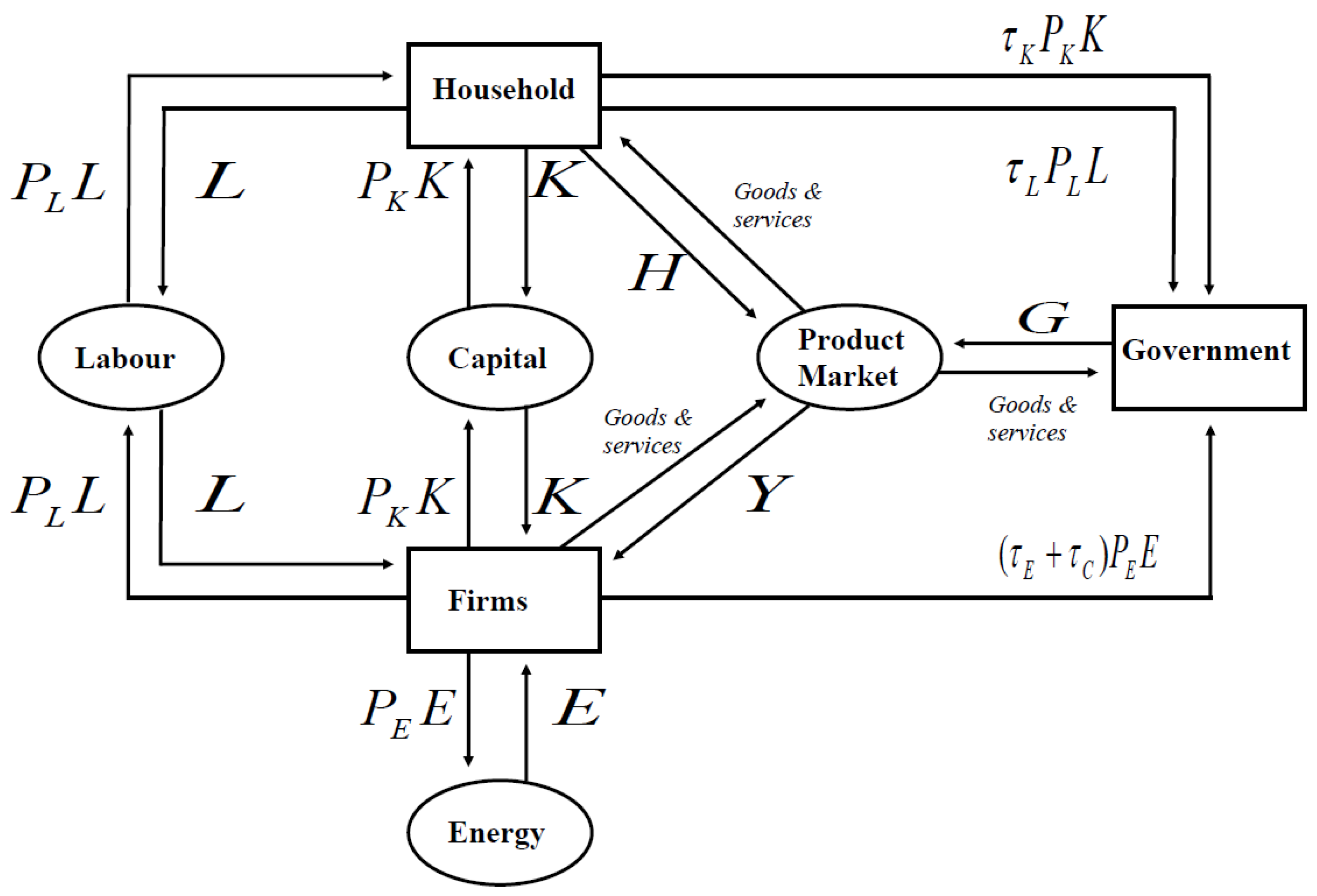
4
A carbon tax can reduce economic growth and increase spending by businesses and households. These effects would have a direct impact on the price of labour, capital, and energy (Winkler and Marquard 2011). In the CGE model, equilibrium is characterised by the set of prices and production levels in each industry, such that the market demand for all goods is equal to the supply. Moreover, the Cobb–Douglas production function was created by Cobb and Douglas (1928) to describe the relationship between manufacturing output, labour input, and capital input for the period 1889–1922 in the U.K. Thus, when these two models are combined, the balance between the carbon tax and governments’, firms’, and households’ expenditure is well-solved.
5
A maximum threshold of carbon tax rate is to protect the fiscal neutral, if the carbon tax rate exceeds this threshold, the fiscal neutral will disappear.
6
A fiscal neutral form of revenue neutrality is that when fiscal revenues from carbon taxes are increased, fiscal revenues from other taxes will decrease, but the government budgetary position will remain unchanged, and the overall tax burden will remain the same.
7
All the parameters are estimated by the method of maximum likelihood estimation (MLE).
8
Prices of labour, capital, and energy are estimated by maximum likelihood estimation (MLE) as endogenous variables.
9
The tax rates including τ L , τ K and τ E & C are endogenous variables, the values of these variables are estimated by the method of maximum likelihood estimation.

References

  1. Abrell, Jan, Anta Ndoye, and Georg Zachmann. 2011. Assessing the Impact of the EU ETS Using Firm Level Data. Bruegel Working Paper 2011/08. Brussels: Bruegel. Available online: https://www.bruegel.org/sites/default/files/wp-content/uploads/imported/publications/WP_2011_08_ETS_01.pdf (accessed on 1 June 2023).
  2. Aghion, Philippe, Ufuk Akcigit, and Jesús Fernández-Villaverde. 2013. Optimal Capital versus Labor Taxation with Innovation-Led Growth. NBER Working Paper No. 19086, (Abrell 2011). pp. 1–38. Available online: https://www.nber.org/papers/w19086 (accessed on 1 June 2023).
  3. Andersen, Mikael S. 2016. An Introductory Note on Carbon Taxation in Europe: A Vermont Briefing. Aarhus: Aarhus University. [Google Scholar]
  4. Andersson, Julius J. 2019. Carbon taxes and CO2 emissions: Sweden as a case study. Economic Policy 11: 1–30. [Google Scholar] [CrossRef] [Green Version]
  5. Atalla, T., and Patrick Bean. 2017. Determinants of energy productivity in 39 countries: An empirical investigation. Energy Economics 62: 217–29. [Google Scholar] [CrossRef]
  6. Bai, Yunfan, and Xing Yang. 2016. The research on the economic effect of market-based environmental policy instruments. Open Journal of Social Sciences 4: 38–47. [Google Scholar] [CrossRef] [Green Version]
  7. Baranzini, Andrea, José Goldemberg, and Stefan Speck. 2000. Survey—A future for carbon taxes. Ecological Economics 32: 395–412. [Google Scholar] [CrossRef]
  8. Baumol, William J. 1972. On taxation and the control of externalities. The American Economic Review 62: 307–22. [Google Scholar]
  9. Baumol, William. J., and Wallace E. Oates. 1971. The use of standards and prices for protection of the environment. The Swedish Journal of Economics 73: 42–54. [Google Scholar] [CrossRef]
  10. Bloomberg New Energy Finance. 2016. Global Trends in Renewable Energy Finance. Available online: https://www.actu-environnement.com/media/pdf/news-26477-rapport-pnue-enr.pdf (accessed on 1 June 2023).
  11. Bonetti, Shanes, and Felix FitzRoy. 1999. Environmental tax reform and government expenditure. Environmental and Resource Economics 13: 289–308. [Google Scholar] [CrossRef]
  12. BP Statistic Review of Global Energy. 2020. Available online: http://www.bp.com/statisticalreview (accessed on 1 June 2023).
  13. Carl, Jeremy, and David Fedor. 2016. Tracking global carbon revenues: A survey of carbon taxes versus cap-and-trade in the real world. Energy Policy 96: 50–77. [Google Scholar] [CrossRef] [Green Version]
  14. Chan, Hei, Shanjun S. Li, and Fan Zhang. 2013. Firm competitiveness and the European Union emissions trading scheme. Energy Policy 63: 1056–64. [Google Scholar] [CrossRef] [Green Version]
  15. Cobb, Charles W., and Paul H. Douglas. 1928. A Theory of Production. American Economic Review 18: 139–65. [Google Scholar]
  16. Commins, N., Seán Lyons, Marc Schiffbauer, and Richard Tol. 2011. Climate policy and corporate behavior. The Energy Journal 32: 51–68. [Google Scholar] [CrossRef] [Green Version]
  17. Convery, Frank J., and Luke Redmond. 2007. Market and Price Developments in the European Union Emissions Trading Scheme. Review of Environmental Economics and Policy 1: 88–111. [Google Scholar] [CrossRef]
  18. Davis, Lucas W., and Lutz Kilian. 2009. Estimating the Effect of a Gasoline Tax on Carbon Emissions. NBER Working Paper No (14685). Cambridge: National Bureau of Economic Research, p. 1. Available online: https://www.nber.org/papers/w14685 (accessed on 1 June 2023).
  19. Dissou, Yazid, Lilia Karnizova, and Qian Sun. 2015. Industry-level econometric estimates of energy-capital-labor substitution with a nested CES production function. International Atlantic Economic Society: Atlantic Economic Journal 43: 107–21. [Google Scholar] [CrossRef]
  20. Ellerman, Denny A., and Barabara Buchner. 2007. The European Union Emissions Trading Scheme: Origins, Allocation, and Early Results. Review of Environmental Economics 1: 66–87. [Google Scholar] [CrossRef]
  21. Global Carbon Project. 2019. Supplemental Data of Global Carbon Budget 2019 (Version 1.0). Available online: https://doi.org/10.18160/gcp-2019 (accessed on 1 June 2023).
  22. Goulder, Lawrence. 1995. Environmental Taxation and the ‘Double Dividend’: A Reader’s Guide. International Tax and Public Finance 2: 157–83. [Google Scholar] [CrossRef]
  23. Huynh, Bao T. 2016. Macroeconomic effects of energy price shocks on the business cycle. Macroeconomic Dynamics 20: 623–42. [Google Scholar] [CrossRef]
  24. IPCC. 2019. United Nations Environment Programme (UNEP) Emissions Gap Report. Available online: https://www.unenvironment.org/resources/emissions-gap-report2019 (accessed on 1 June 2019).
  25. Jorgenson, D. 2014. Time to Tax Carbon. Harvard Magazine. pp. 52–56, 78–79. Available online: http://bit.ly/1dDlxtI (accessed on 1 June 2023).
  26. Jorgenson Dale, Richard Goettle, Ho Mun, and Peter Wilcoxen. 2013. Double Dividend: Environmental Taxes and Fiscal Reform in the United States. Cambridge and London: MIT Press. [Google Scholar]
  27. Jorgenson, Dale W., Daniel T. Slesnick, Peter J. Wilcoxen, Paul L. Joskow, and Raymond Kopp. 1992. Carbon taxes and economic welfare. Brookings Papers on Economic Activity 1992: 393–454. [Google Scholar] [CrossRef] [Green Version]
  28. Krupnick, Alan, Ian Parry, Margaret Walls, Tony Knowles, and Kristin Hayes. 2010. Towards a New National Energy Policy: Assessing the Options. Washington, DC: Resources for the Future and National Energy Policy Institute. [Google Scholar]
  29. Lai, C. F. 2016. Examining the double dividend effect of energy tax with the overlapping generations model. International Journal of Energy Economics and Policy 6: 53–57. [Google Scholar]
  30. Larsen, Kate, Trevor Houser, and Shashank Mohan. 2019. Sizing Up a Potential Fuel Economy Standards Freeze. Available online: htpps://rhg.com/research/sizing-up-a-potential-fuel-economy-standards-freeze (accessed on 29 June 2023).
  31. Li, Wei, and Zhijie J. Jia. 2017. Carbon tax, emission trading, or the mixed policy: Which is the most effective strategy for climate change mitigation in China? Mitigation and Adaption Strategies for Global Change 22: 973–92. [Google Scholar] [CrossRef]
  32. Liang, Q. M., and Y. M. Wei. 2012. Distributional impacts of taxing carbon in China: Results from the CEEPA model. Applied Energy 92: 545–51. [Google Scholar] [CrossRef]
  33. Mankiw, N. Gregory, David Romer, and David N. Weil. 1992. A contribution to the empirics of economic growth. The Quarterly Journal of Economics 107: 407–37. [Google Scholar] [CrossRef]
  34. Mardones, C., and B. Flores. 2018. Effectiveness of a CO2 tax on industrial emissions. Energy Economics 71: 370–82. [Google Scholar] [CrossRef]
  35. Marron, Donald, and Eric J. Toder. 2014. Tax policy issues in designing a carbon tax. American Economic Review: Papers & Proceedings 104: 563–68. [Google Scholar]
  36. Marron, Donald, Eric J. Toder, and Lydia Austin. 2015. Taxing Carbon: What, Why and How. Washington, DC: Tax Policy Center. Urban Institute Brooking Institution, pp. 1–28. [Google Scholar]
  37. Martin, Ralf, Mirabelle Muûls, and Ulrich Wagner. 2016. The Impact of the European Union Emissions Trading Scheme on Regulated Firms: What Is the Evidence after Ten Years? Review of Environmental Economics and Policy 10: 129–48. [Google Scholar] [CrossRef] [Green Version]
  38. Masanjala, Winford H., and Chris Papageorgiou. 2004. The Solow model with CES technology: Nonlinearities and parameter heterogeneity. Journal of Applied Econometrics 19: 171–201. [Google Scholar] [CrossRef]
  39. Masoud, Yahoo, and Jamal Othman. 2017. Carbon and energy taxation for CO2 mitigation: A CGE model of Malaysia. Environmental Development and Sustainability 19: 239–62. [Google Scholar]
  40. McKibbin, Warwick, Adele C. Morris, Peter J. Wilcoxen, and Yiyong Y. Cai. 2015. Carbon taxes and U.S. fiscal reform. National Tax Journal 68: 139–56. [Google Scholar] [CrossRef] [Green Version]
  41. McKitrick, Ross, Elmira Aliakbari, and Ashley Stedman. 2019. The Impact of the Federal Carbon Tax on the Competitiveness of Canadian Industries. Fraser Institute, August 22. Available online: https://www.fraserinstitute.org/studies/impact-of-the-federal-carbon-tax-on-the-competitiveness-of-canadian-industries (accessed on 1 June 2023).
  42. Meng, Xanming, Mahinda Siriwardana, and Judith McNeill. 2015. The environmental and employment effect of Australian carbon tax. International Journal of Social Science and Humanity 5: 514–19. [Google Scholar] [CrossRef] [Green Version]
  43. Miller, Sebastián J., and Mauricio A. Vela. 2013. Are Environmentally Related Taxes Effective? IDB Working Paper Series No. IDB-WP-467. Inter-American Development Bank, pp. 1–27. Available online: https://core.ac.uk/display/19456380 (accessed on 1 June 2023).
  44. Natural Resources Defense Council. 2018. Comments of the Natural Resources Defense Council on EPA’s Proposed Emission Guidelines for Greenhouse Gas Emissions From Existing Electric Utility Generating Units; Revisions to Emission Guideline Implementing Regulations. Available online: https://www.nrdc.org/sites/default/files/nrdc-ace-comments-20181031.pdf (accessed on 1 June 2023).
  45. Nordhaus, William. 2010. Carbon Taxes to Move Toward Fiscal Sustainability. The Economists’ Voice 7: 3. Available online: http://bit.ly/1LUcSxO (accessed on 1 June 2023). [CrossRef]
  46. Nunavut. 2019. The Carbon Tax in Nunavut Frequently Asked Questions. FAQ-Carbon Tax in Nunavut. Available online: https://gov.nu.ca/finance/documents/carbon-tax-frequently-asked-questions (accessed on 1 June 2023).
  47. Nurdianto, Ditya A., and Budy Resosudarmo. 2016. The economy-wide impact of a uniform carbon tax in ASEAN. Journal of Southeast Asian Economies 33: 1–22. [Google Scholar] [CrossRef]
  48. Oberndorfer, Ulrich, and Klauss Rennings. 2007. Costs and Competitiveness Effects of the European Union Emissions Trading Scheme. European Environment 17: 1–17. [Google Scholar] [CrossRef]
  49. Othman, Jamal, and Masoud Yahoo. 2014. Reducing CO2 emissions in Malaysia: Do carbon taxes work? Prosiding Persidangan Kebangsaan Ekonomi Malaysia Ke 9: 175–82. [Google Scholar]
  50. Pang, Y. 2019. Taxing pollution and profits: A bargaining approach. Energy Economics 78: 278–88. [Google Scholar] [CrossRef]
  51. Pearce, David. 1991. The Role of Carbon Taxes in Adjusting to Global Warming. Economic Journal 101: 938–48. [Google Scholar] [CrossRef]
  52. Pereira, Alfredo M., Rui M. Pereira, and Pedro G. Rodrigues. 2016. A new carbon tax in Portugal: A missed opportunity to achieve the triple dividend? Energy Policy 9: 110–18. [Google Scholar] [CrossRef] [Green Version]
  53. Poterba, James M. 1991. Tax Policy to Combat Global Warming: On Designing a Carbon Tax. MIT-CEPR 91-003WP. MIT Center for Energy and Environmental Policy Research, March. Available online: https://www.nber.org/papers/w3649 (accessed on 1 June 2023).
  54. Rosenberg, Joseph, Eric Toder, and Chenxi Lu. 2018. Distributional Implications of a Carbon Tax. New York: Center on Global Energy Policy, p. 3. [Google Scholar]
  55. Rosendahl, Knut E. 1995. Carbon Taxes and the Petroleum Wealth; Cleveland: International Association for Energy Economics. Available online: https://www.osti.gov/biblio/416359-carbon-taxes-petroleum-wealth (accessed on 1 June 2023).
  56. Saboori, Behnaz, and Jamalludin B. Sulaiman. 2013. Environmental degradation, economic growth and energy consumption: Evidence of the environmental Kuznets curve in Malaysia. Energy Policy 60: 892–905. [Google Scholar] [CrossRef]
  57. Schneider, Uwe A., and Bruce A. McCarl. 2005. Implications of a Carbon Based Energy Tax for U.S. Agriculture. Agricultural and Resource Economics Review 34: 265–79. [Google Scholar] [CrossRef] [Green Version]
  58. Scrimgeour, Frank G., Les Oxley, and Koli Fatai. 2004. Reducing carbon emissions? The relative effectiveness of different types of environmental tax: The case of New Zealand. Paper presented at 2nd International Congress on Environmental Modeling and Software, Osnabruck, Germany, June 10–14; Available online: https://scholarsarchive.byu.edu/iemssconference/2004/all/172/ (accessed on 1 June 2023).
  59. Solow, R. M. 1956. A contribution to the theory of economic growth. The Quarterly Journal of Economics 71: 65–94. [Google Scholar] [CrossRef]
  60. Stern, Nicholas. 2007. The Economics of Climate Change: The Stern Review. Cambridge: Cambridge University Press. [Google Scholar]
  61. Stern, Todd. 2010. United States Association with Copenhagen Accord. Washington, DC: United States Department of State, Office of the Special Envoy for Climate Change, January 28, Available online: https://unfccc.int/files/meetings/cop_15/copenhagen_accord/application/pdf/unitedstatescphaccord_app.1.pdf (accessed on 1 June 2019).
  62. Swan, Trevor W. 1956. Economic growth and capital accumulation. Economic Record 32: 334–61. [Google Scholar] [CrossRef]
  63. Symons, Elizabeth, John Proops, and Philip Gay. 1994. Carbon taxes, consumer demand and carbon dioxide emissions: A simulation analysis for the UK. Fiscal Studies 15: 19–43. [Google Scholar] [CrossRef]
  64. Tol, Richard S. J. 2012. Leviathan carbon taxes in the short run: A letter. Climatic Change 114: 409–15. [Google Scholar] [CrossRef]
  65. Torrie, Ralph D., Christopher Stone, and David B. Layzell. 2016. Understanding energy systems change in Canada: 1. Decomposition of total energy intensity. Energy Economics 5: 101–6. [Google Scholar] [CrossRef] [Green Version]
  66. United Nations. 2016. Paris Agreement. Available online: https://unfccc.int/sites/default/files/english_paris_agreement.pdf (accessed on 1 June 2023).
  67. Upmann, Thorsten. 2009. A positive analysis of labor-market institutions and tax reforms. International Tax and Public Finance 16: 621–46. [Google Scholar] [CrossRef]
  68. US Energy Information Administration (EIA). 2021. Energy Explained, Your Guide to Understanding. Available online: https://www.eia.gov/energyexplained (accessed on 1 June 2023).
  69. Wara, Michael. 2015. Instrument choice, carbon emissions, and information. Michigan Journal of Environmental and Administrative Law 4: 261–302. [Google Scholar] [CrossRef]
  70. Winkler, Harald, and Andrew Marquard. 2011. Analysis of the economic implications of a carbon tax. Journal of Energy in Southern Africa 22: 55–68. [Google Scholar] [CrossRef] [Green Version]
  71. World Bank. 2020. Data Indicators from the Website of The World Bank. Available online: https://data.worldbank.org/indicator (accessed on 1 June 2023).
  72. Yukon. 2019. Proposed Framework: Yukon Government Carbon Price Rebate. Yukon Government. January 17. Available online: https://yukon.ca/en/proposed-framework-government-yukon-carbon-price-rebate (accessed on 1 June 2023).
  73. Zachariadis, Theodoros. 2015. How can Cyprus meet its energy and climate policy commitments? The importance of a carbon tax. December. Cyprus Economic Policy Review 9: 3–20. [Google Scholar]
  74. Zhang, Kezhong, Juan Wang, and Yongming Huang. 2011. Estimating the effect of carbon tax on CO2 emissions of coal in China. Journal of Environmental Protection 2: 1101–07. [Google Scholar] [CrossRef] [Green Version]
  75. Zhao, Yibing, Can Wang, Yuwei Sun, and Xianbing Liu. 2018. Factors influencing companies’ willingness to pay for carbon emissions: Emission trading schemes in China. Energy Economics 75: 357–67. [Google Scholar] [CrossRef]
Figure 1. Primary energy consumption by source (terawatt hours (TWh), United States, 1965 to 2018. Source: BP Statistic Review of Global Energy (2020).
Jrfm 16 00317 g001
Figure 2. The renewable energy investment rate (as % of GDP) for nine economies in G20 in 2015. Source: Bloomberg New Energy Finance (2016).
Jrfm 16 00317 g002
Figure 3. The relationship between labour, capital, energy, firms, government, and households.
Jrfm 16 00317 g003
Figure 4. The technical progress function e Y 0 ( x ) impacted on the production of firms in the U.S. during 1990–2014.
Jrfm 16 00317 g004
Figure 5. The technical progress function e G 0 ( x ) impacted on the expenditure of government in the U.S. during 1990–2014.
Jrfm 16 00317 g005
Figure 6. The technical progress function e H 0 ( x ) impacted on the expenditure of household in the U.S. during 1990–2014.
Jrfm 16 00317 g006
Figure 7. Dynamic variance curves of σ Y , t ,   σ G , t , σ H , t from GARCH(1,1) models in the U.S. during 1990–2014.
Jrfm 16 00317 g007
Figure 8. The estimated annual wages   P L in the unit of USD/1 person in the U.S. during 1990–2014.
Jrfm 16 00317 g008
Figure 9. The estimated capital price P K   in the unit of USD/USD 1 capital formation in the U.S. during 1990–2014.
Jrfm 16 00317 g009
Figure 10. The estimated annual price of oil equivalent energy P E   in the unit of USD/1 barrel in the U.S. during 1990–2014.
Jrfm 16 00317 g010
Figure 11. The estimated annual carbon price P C   in the unit of USD/kg CO2 in the U.S. during 1990–2014.
Jrfm 16 00317 g011
Table 1. Basic statistical data of the United States.
Year Y G H L K E C O 2 θ C
GDP USD
in Billions
Govt USD
in Billions
Household Cons USD
in Billions
Labor
in Millions
Gross Capital USD
in Billions
Energy KGs
in Billions
KGs
in Billions
kg per kg of Energy
19905979.59947.993825.63127.941283.821915.054823.402.52
19916174.041004.073960.15128.701238.441930.624820.852.50
19926539.301049.254215.65130.851309.131969.364909.532.49
19936878.721074.184471.00132.281398.712003.845028.672.51
19947308.761109.574741.02134.621550.662041.295094.352.50
19957664.061144.484984.18136.501625.162067.325132.922.48
19968100.201176.505268.07138.421752.012113.255252.112.49
19978608.521224.635560.72140.841925.132134.525368.722.52
19989089.171272.115903.03142.832076.732152.685401.012.51
19999660.621357.576307.02144.822252.662210.905504.672.49
200010,284.781444.176792.40146.772424.012273.345693.682.50
200110,621.821545.137103.10147.742342.272230.705595.792.51
200210,977.511651.367384.05148.572368.572255.945641.312.50
200311,510.671755.597765.53149.182493.212261.175675.702.51
200412,274.931868.948260.02150.262765.142307.775756.082.49
200513,093.731980.058794.11152.123040.752318.775789.732.50
200613,855.892089.859303.99153.993233.002296.825697.292.48
200714,477.642209.729750.51155.293235.952337.005789.032.48
200814,718.582368.5710,013.65157.093059.442277.085614.112.47
200914,418.742442.069846.97157.202525.142164.825263.512.43
201014,964.372522.2110,202.19157.022752.642215.225395.532.44
201115,517.932530.8610,689.30157.132877.762190.425289.682.41
201216,155.262544.1511,050.63158.433126.142156.985119.442.37
201316,691.522523.7311,361.17159.013298.622182.585159.162.36
201417,427.612562.6911,863.67159.803510.762216.195254.282.37
Table 2. Three models for firms’ production, government, and household expenditure in the United States during 1990–2014.
M o d e l T 0 ( x t ) T 1 ( x t ) T 2 ( x t ) T 3 ( x t ) l n L t l n K t l n E t
l n Y t y 0 = 6.677636
( p = 0.0000   * * * )
y 1 = 0.355981
( p = 0.0000   * * * )
y 2 = 0.002686
( p = 0.0000   * * * )
y 3 = 0.018067
( p = 0.0000   * * * )
α = 0.529271
( p = 0.0000   * * * )
β = 0.195832
( p = 0.0000   * * * )
γ = 0.274897
( p = 0.0000   * * * )
l n G t g 0 = 1.682684
( p = 0.0000   * * * )
g 1 = 0.346872
( p = 0.0000   * * * )
g 2 = 0.049443
( p = 0.0000   * * * )
g 3 = 0.108124
( p = 0.0000   * * * )
ξ = 0.202961
( p = 0.0000   * * * )
ζ = 0.194868
( p = 0.0030   * * * )
ς = 0.602171
( c o n t r o l )
l n H t h 0 = 8.381027
( p = 0.0000   * * * )
h 1 = 0.378485
( p = 0.0000   * * * )
h 2 = 0.008665
( p = 0.0000   * * * )
h 3 = 0.013608
( p = 0.0000   * * * )
m = 0.749962   ( c o n t r o l ) n = 0.249951   ( c o n t r o l )
Notes: (1) *** represents that the estimated coefficients are significant at the confidence level of 1%; (2) ς = 0.602171 is from the market clearing condition of firms, government and household; (3) m = 0.749962 and n = 0.249951 are from the market clearing condition of firms, government and household, theoretically, m + n = 1 , hear m + n = 0.999914 .
Table 3. Three GARCH(1,1) models for firms, government, and household of the United States during 1990–2014.
Variance 1 a t 1 2 σ t 1 2 Residual   a t is from the Equation of
σ t 2 ω 0 = 0.003188
( p = 0.6899 )
ω 1 = 0.095786
( p = 0.7714 )
ω 2 = 0.800057
( p = 0.0000   * * * )
l n Y t
σ t 2 ω 0 = 0.000638
( p = 0.9992 )
ω 1 = 0.100016
( p = 0.8593 )
ω 2 = 0.899921
( p = 0.0000   * * * )
l n G t
σ t 2 ω 0 = 0.000107
( p = 0.9983 )
ω 1 = 0.099986
( p = 0.8037 )
ω 2 = 0.899906
( p = 0.0000   * * * )
l n H t
Notes: (1) *** represents that the estimated coefficients are significant at the confidence level of 1%.
Table 4. Empirical results of prices of labour, capital, energy, and carbon dioxide in the United States during 1990–2014.
Variable P L P K P E P E P E P E θ C P C = P E / θ C
Year U S D p e r s o n U S D U S D U S D k g   o i l _ e U S D b a r r e l   o i l _ e U S D g a l l o n   o i l _ e U S D l i t r e   o i l _ e k g   C O 2 k g   o i l _ e U S D k g   C O 2
199024,7370.91210.629792.55892.20380.58212.51870.2500
199125,3910.97630.626792.10632.19300.57932.49710.2510
199226,4510.97820.647195.11342.26460.59822.49300.2596
199327,5230.96310.665597.81512.32890.61522.50950.2652
199428,7360.92300.7143104.99482.49990.66032.49570.2862
199529,7160.92350.7427109.16372.59910.68662.48290.2991
199630,9720.90540.7835115.15332.74170.72422.48530.3152
199732,3500.87570.8541125.54262.98910.78962.51520.3396
199833,6800.85710.8891130.68663.11160.82192.50900.3544
199935,3060.83980.9028132.69753.15950.83462.48980.3626
200037,0890.83090.9010132.42603.15300.83292.50450.3597
200138,0520.88810.8847130.04053.09620.81792.50850.3527
200239,1070.90760.8609126.53383.01270.79582.50060.3443
200340,8370.90410.8799129.32593.07920.81342.51010.3505
200443,2370.86930.9299136.67693.25420.85962.49420.3728
200545,5580.84331.0003147.03233.50080.92472.49690.4006
200647,6230.83931.0719157.55533.75130.99092.48050.4321
200749,3420.87621.0772158.32843.76970.99582.47710.4349
200849,5900.94211.0260150.80893.59070.94852.46550.4162
200948,5451.11820.9838144.59803.44280.90942.43140.4046
201050,4421.06461.0112148.62403.53870.93472.43570.4152
201152,2701.05601.0490154.18533.67110.96972.41490.4344
201253,9711.01201.1871174.47764.15421.09732.37340.5001
201355,5590.99091.2859189.00634.50021.18872.36380.5440
201457,7220.97211.3542199.04894.73931.25192.37090.5712
Notes: (1) 1 tonne = 1000 kg; (2) 1 barrel = 146.9819432 kg; (3) 1 U.S. gallon = 3.499570077 kg; (4) 1 litre = 0.924414737 kg; (5) all these units are suitable for oil equivalent; (6) oil _ e represents oil equivalent.
Table 5. Empirical results of tax rates (%) and taxes (USD) of labour, capital, and energy in the United States during 1990–2014.
Variable τ L τ K τ E & C P L L P K K P E E τ L P L L τ K P K K τ E & C P E E
Year%%% U S D U S D   i n   B i l l i o n s U S D   i n   B i l l i o n s U S D   i n   B i l l i o n s U S D   i n   B i l l i o n s U S D   i n   B i l l i o n s
19906.08%15.78%53.21%3164.821171.001205.97192.41184.73641.64
19916.24%16.18%55.34%3267.741209.081209.82203.79195.66669.49
19926.15%15.97%54.20%3461.061280.601274.39212.96204.47690.68
19935.99%15.54%51.99%3640.711347.071333.54218.02209.32693.34
19945.82%15.11%49.82%3868.311431.291458.17225.20216.22726.53
19955.73%14.86%48.61%4056.371500.871535.40232.29223.02746.42
19965.57%14.45%46.66%4287.201586.281655.63238.78229.26772.55
19975.46%14.16%45.27%4556.241685.821823.17248.55238.64825.32
19985.37%13.93%44.21%4810.641779.951914.02258.19247.89846.26
19995.39%13.98%44.47%5113.091891.861996.03275.53264.55887.69
20005.38%13.97%44.42%5443.442014.092048.21293.11281.42909.88
20015.58%14.48%46.77%5621.832080.091973.59313.60301.10923.00
20025.77%14.97%49.15%5810.082149.751942.10335.16321.80954.50
20035.85%15.18%50.17%6092.272254.161989.55356.32342.11998.20
20045.84%15.15%50.04%6496.772403.822145.97379.32364.201073.90
20055.80%15.05%49.53%6930.132564.172319.57401.87385.851148.97
20065.78%15.01%49.34%7333.522713.432462.05424.16407.241214.80
20075.85%15.19%50.23%7662.602835.192517.41448.49430.601264.42
20086.17%16.01%54.44%7790.122882.372336.37480.73461.561271.97
20096.49%16.85%58.98%7631.422823.652129.71495.64475.881256.18
20106.46%16.77%58.53%7920.212930.502239.97511.91491.501311.08
20116.25%16.23%55.58%8213.193038.912297.77513.67493.181277.19
20126.04%15.67%52.66%8550.513163.722560.48516.36495.771348.46
20135.80%15.05%49.52%8834.343268.732806.62512.22491.791389.91
20145.64%14.63%47.52%9223.933412.883001.25520.13499.391426.11
Table 6. The reduction targets of CO2 emissions and empirical results in the United States during 2005–2050.
Variable ϕ t ϕ t ϕ t C t c t E t θ t E C l e a n , t E C l e a n , t / E t
YearTarget
%
Yearly
%
% k g   C O 2   i n   B i l l i o n s % k g   o i l _ e in Billions k g   C O 2 k g   o i l _ e k g   c l e a n in Billions k g   c l e a n k g   o i l _ e
2005 5724.110.585%2318.772.4969
2006 −1.133%−1.133%5658.50−1.133%2296.822.4922
2007 −1.133%−2.267%5592.88−1.146%2337.002.4213
2008 −1.133%−3.400%5527.27−1.160%2277.082.4562
2009 −1.133%−4.533%5461.65−1.173%2164.822.5532
2010 −1.133%−5.666%5396.04−1.187%2215.222.46556.680.0030
2011 −1.133%−6.800%5330.42−1.201%2190.422.46358.400.0038
2012 −1.133%−7.933%5264.81−1.216%2156.982.47121.500.0007
2013 −1.133%−9.066%5199.19−1.231%2182.582.412253.640.0246
2014 −1.133%−10.200%5133.58−1.246%2216.192.3460113.770.0513
2015 −1.133%−11.333%5067.96−1.262%2229.542.3025153.660.0689
2016 −1.133%−12.466%5002.35−1.278%2242.982.2595193.630.0863
2017 −1.133%−13.600%4936.73−1.295%2256.492.2169233.680.1036
2018 −1.133%−14.733%4871.12−1.312%2270.092.1747273.810.1206
2019 −1.133%−15.866%4805.47−1.329%2283.772.1329314.020.1375
2020−17.00%−1.133%−17.000%4654.94−1.348%2297.532.0916354.330.1542
2021 −2.600%−19.600%4504.41−3.133%2311.382.0139429.040.1856
2022 −2.600%−22.200%4353.87−3.234%2325.311.9371503.840.2167
2023 −2.600%−24.800%4203.34−3.342%2339.321.8612578.730.2474
2024 −2.600%−27.400%4052.81−3.457%2353.411.7861653.700.2778
2025−30.00%−2.600%−30.000%3913.86−3.581%2367.601.7118728.750.3078
2026 −2.400%−32.400%3774.90−3.429%2381.861.6432799.200.3355
2027 −2.400%−34.800%3635.95−3.550%2396.221.5754869.750.3630
2028 −2.400%−37.200%3497.00−3.681%2410.661.5083940.380.3901
2029 −2.400%−39.600%3358.04−3.822%2425.181.44201011.090.4169
2030−42.00%−2.400%−42.000%3239.35−3.974%2439.801.37641081.890.4434
2031 −2.050%−44.050%3120.66−3.534%2454.501.31981144.590.4663
2032 −2.050%−46.100%3001.97−3.664%2469.291.26381207.380.4890
2033 −2.050%−48.150%2883.28−3.803%2484.171.20841270.250.5113
2034 −2.050%−50.200%2764.59−3.954%2499.141.15371333.220.5335
2035 −2.050%−52.250%2645.91−4.116%2514.201.09961396.270.5554
2036 −2.050%−54.300%2527.22−4.293%2529.351.04611459.420.5770
2037 −2.050%−56.350%2408.53−4.486%2544.590.99321522.650.5984
2038 −2.050%−58.400%2289.84−4.696%2559.930.94091585.980.6195
2039 −2.050%−60.450%2171.15−4.928%2575.350.88911649.400.6405
2040 −2.050%−62.500%2052.46−5.183%2590.870.83801712.920.6611
2041 −2.050%−64.550%1933.77−5.467%2606.480.78741776.520.6816
2042 −2.050%−66.600%1815.08−5.783%2622.190.73751840.230.7018
2043 −2.050%−68.650%1696.39−6.138%2637.990.68811904.020.7218
2044 −2.050%−70.700%1577.70−6.539%2653.890.63921967.910.7415
2045 −2.050%−72.750%1459.01−6.997%2669.880.59092031.900.7610
2046 −2.050%−74.800%1340.32−7.523%2685.970.54322095.980.7803
2047 −2.050%−76.850%1221.63−8.135%2702.150.49602160.160.7994
2048 −2.050%−78.900%1102.94−8.855%2718.440.44942224.440.8183
2049 −2.050%−80.950%984.25−9.716%2734.820.40332288.820.8369
2050−83.00%−2.050%−83.000%5724.11−10.761%2751.300.35772353.290.8553
Table 7. Carbon tax rates in the units of USD/kg CO2 and percentages for reduction targets in the United States during 2005–2050.
Variable T C , t T C , t τ C , t τ E , t τ C , t / τ E & C , t τ E , t / τ E & C , t τ E & C , t P C , t η t
Year U S D k g   C O 2 U S D t o n n e   C O 2 %%%%% U S D k g   C O 2 Ratio
20050.00000.00.00%49.53%0.00%100.00%49.53%0.40060.0000
20060.00242.40.55%47.88%1.13%98.87%48.43%0.43010.0115
20070.00484.81.07%46.29%2.27%97.73%47.36%0.44490.0232
20080.00727.21.74%49.30%3.40%96.60%51.03%0.41770.0352
20090.00989.82.54%53.45%4.53%95.47%55.99%0.38530.0475
20100.012412.43.02%50.21%5.67%94.33%53.23%0.41010.0601
20110.015015.03.53%48.36%6.80%93.20%51.89%0.42580.0730
20120.017717.73.69%42.87%7.93%92.07%46.57%0.48040.0862
20130.020520.53.85%38.63%9.07%90.93%42.48%0.53310.0997
20140.023423.44.05%35.68%10.20%89.80%39.73%0.57730.1136
20150.026326.36.60%51.63%11.33%88.67%58.23%0.39880.1278
20160.029329.37.22%50.67%12.47%87.53%57.88%0.40640.1424
20170.032432.47.82%49.71%13.60%86.40%57.54%0.41430.1574
20180.035635.68.43%48.77%14.73%85.27%57.19%0.42230.1728
20190.038838.89.02%47.83%15.87%84.13%56.85%0.43060.1886
20200.042242.29.61%46.90%17.00%83.00%56.51%0.43910.2048
20210.050250.211.01%45.16%19.60%80.40%56.17%0.45600.2438
20220.058858.812.40%43.44%22.20%77.80%55.84%0.47410.2853
20230.067967.913.76%41.74%24.80%75.20%55.50%0.49340.3298
20240.077777.715.12%40.05%27.40%72.60%55.17%0.51420.3774
20250.088388.316.45%38.39%30.00%70.00%54.84%0.53650.4286
20260.098798.717.66%36.85%32.40%67.60%54.51%0.55890.4793
20270.1099109.918.86%35.33%34.80%65.20%54.18%0.58290.5337
20280.1220122.020.04%33.82%37.20%62.80%53.86%0.60890.5924
20290.1350135.021.20%32.34%39.60%60.40%53.54%0.63690.6556
20300.1491149.122.35%30.86%42.00%58.00%53.22%0.66720.7241
20310.1621162.123.30%29.60%44.05%55.95%52.90%0.69580.7873
20320.1761176.124.24%28.34%46.10%53.90%52.58%0.72670.8553
20330.1912191.225.17%27.10%48.15%51.85%52.26%0.75990.9286
20340.2076207.626.08%25.87%50.20%49.80%51.95%0.79601.0080
20350.2253225.326.98%24.66%52.25%47.75%51.64%0.83521.0942
20360.2447244.727.87%23.46%54.30%45.70%51.33%0.87791.1882
20370.2659265.928.75%22.27%56.35%43.65%51.02%0.92471.2910
20380.2891289.129.62%21.10%58.40%41.60%50.72%0.97611.4038
20390.3148314.830.48%19.94%60.45%39.55%50.41%1.03281.5284
20400.3432343.231.32%18.79%62.50%37.50%50.11%1.09591.6667
20410.3750375.032.15%17.66%64.55%35.45%49.81%1.16621.8209
20420.4106410.632.98%16.54%66.60%33.40%49.51%1.24531.9940
20430.4510451.033.79%15.43%68.65%31.35%49.22%1.33472.1898
20440.4969496.934.59%14.33%70.70%29.30%48.92%1.43672.4130
20450.5498549.835.38%13.25%72.75%27.25%48.63%1.55412.6697
20460.6113611.336.16%12.18%74.80%25.20%48.34%1.69062.9683
20470.6836683.636.93%11.12%76.85%23.15%48.05%1.85143.3197
20480.7701770.137.68%10.08%78.90%21.10%47.76%2.04353.7393
20490.8751875.138.43%9.04%80.95%19.05%47.47%2.27714.2493
20501.00551005.539.17%8.02%83.00%17.00%47.19%2.56714.8824
Disclaimer/Publisher’s Note: The statements, opinions and data contained in all publications are solely those of the individual author(s) and contributor(s) and not of MDPI and/or the editor(s). MDPI and/or the editor(s) disclaim responsibility for any injury to people or property resulting from any ideas, methods, instructions or products referred to in the content.

