1. Introduction
The increasing utilization of sentiment analysis (SA) for obtaining a sentiment index holds promise as an approach for predicting commodity prices and foreign exchange rates. By analyzing unstructured data such as social media posts, news articles, and other textual data, SA provides insights into public opinions and market sentiment, enabling price prediction (
Smailović et al. 2013). Utilizing a sentiment index, rather than relying on a large dataset of indicators, offers several advantages, including simplifying the modeling process and reducing the risk of overfitting. SA also offers a more up-to-date perspective on market sentiment, as it captures real-time changes in public opinion and market sentiment (
Philander and Zhong 2016). However, while a sentiment index proves valuable in predicting short-term fluctuations (
Qiu et al. 2022) in commodity and foreign exchange markets, long-term trends in these markets are more significantly influenced by factors such as macroeconomic indicators and political events. Hence, while SA presents a promising approach to prediction, we must also consider its limitations and potential biases and supplement SA with other relevant data sources and indicators.
Hence, the primary objectives of this research are as follows: First, to analyze whether sentiment indicators derived from sentiment analysis techniques can outperform a large dataset of indicators when employing machine learning and deep learning methods for prediction. Second, to verify whether machine learning models, which have gained considerable attention, genuinely exhibit better prediction capabilities than classical ARIMA models. Third, to apply our proposed hybrid model to commodity gold futures prices and foreign exchange rates, evaluate their prediction performance, and compare them with the aforementioned machine learning and classical statistical approaches.
This study is divided into three steps. In the first step, we perform sentiment analysis on the collected unstructured news headlines to obtain a sentiment index (referred to as the SI dataset). Then, we calculate technical indicators and collect other relevant indicators from stock markets, bond markets, commodity markets, and foreign exchange markets to create a multivariate dataset (referred to as the large dataset). In the second step, we apply moving window machine learning approaches (RF, XGB, and LSTM) and a classical statistical model (ARIMA) to these two datasets to evaluate their prediction performance using the root mean squared error (RMSE), mean absolute percentage error (MAPE), and mean absolute error (MAE). In the third step, we propose several decompositions and transformations integrated with statistical and machine learning approaches, such as seasonal-decomposition-ARIMA-LSTM, wavelet-ARIMA-LSTM, wavelet-ARIMA-RF, and wavelet-ARIMA-XGB. Specifically, we first transform and decompose the time series into linear and nonlinear parts or dynamic levels and noise parts. Then, we apply classical ARIMA to predict the linear and dynamic levels and use RF, XGB, and LSTM machine/deep learning approaches to predict the nonlinear and noise parts. We evaluate our proposed approaches using RMSE, MAPE, and MAE and compare the prediction results with the aforementioned forecasting. Additionally, we perform walk-forward testing to validate the effectiveness of the triple-combination approaches. To assess any statistically significant differences between our proposed approach and the ARIMA model, we utilize the modified Diebold–Mariano test statistic. This comprehensive testing methodology provides further insights into the performance and comparative analysis of the proposed approaches.
The main findings of this study are as follows: First, the combination of the sentiment indicator with the moving window LSTM machine learning model demonstrates outstanding forecasting performance. Second, the sentiment indicator dataset used in conjunction with the moving window machine learning and deep learning models does not surpass the performance of the traditional ARIMA model. Third, our proposed triple-combination approaches exhibit superior prediction performance compared to either the machine learning models or the ARIMA model when forecasting commodity gold futures prices and euro foreign exchange rates. Lastly, although the sentiment indicator dataset does not outperform the prediction accuracy of the ARIMA model, our empirical results indicate that the sentiment dataset is more accurate in predicting commodity prices and foreign exchange rates than the large dataset, which comprises various indicators.
To the best of our knowledge, this study is the first to investigate whether sentiment indicators can replace a large dataset of indicators in forecasting commodity prices and foreign exchange rates. Moreover, this study introduces a novel approach by combining data decomposition with machine learning models and classical statistical models to predict prices in commodity and foreign exchange markets. Additionally, the proposed triple-combination approaches demonstrate higher accuracy compared to the individual models. These findings offer new insights and potential predictors for investors and policymakers.
The rest of this paper is organized as follows:
Section 2 reviews the literature.
Section 3 provides a detailed description of the study’s data, methodologies, and evaluation measures.
Section 4 presents and analyzes the empirical results. Finally,
Section 5 concludes the study.
2. Literature Review
The contribution of
Bedi and Khurana (
2019) is focused on improving SA prediction for textual data by incorporating fuzziness with deep learning.
Ito et al. (
2019) and
Ito et al. (
2020) propose a novel neural network model called the contextual sentiment neural network (CSNN) model, which offers insights into the SA prediction process and utilizes an initialization propagation (IP) learning strategy. Leveraging SA on Twitter tweets,
Naeem et al. (
2021) suggest a machine learning-based strategy for forecasting exchange rates. Their findings demonstrate that SA can facilitate the prediction of foreign exchange rates, particularly the US dollar against the Pakistani rupee.
Li et al. (
2016) acknowledge the usefulness of online data, including news releases and social media networks such as Twitter, in forecasting price changes.
Xiang et al. (
2021) propose a Chinese Weibo SA algorithm that combines the BERT (Bidirectional Encoder Representations from Transformers) model and the Hawkes process to effectively monitor changes in users’ emotional states and perform SA on Weibo. However, limited studies have examined whether sentiment indicators can replace large sets of index data for forex prediction. If sentiment indicators can effectively replace a substantial amount of index datasets and achieve comparable or better forecasting performance, it could significantly enhance forecasting efficiency and provide valuable insights to investors and decision-makers.
Moreover, in recently published research, the use of rapidly developing machine and deep learning modeling techniques for forecasting time series is one of the most extensively researched topics in the academic literature (
Bakay and Ağbulut 2021;
Bouktif et al. 2018;
Wang and Wang 2016;
Amat et al. 2018;
Chatzis et al. 2018;
Farsi et al. 2021;
Zhang and Hamori 2020;
Plakandaras et al. 2015;
Luo et al. 2019;
McNally et al. 2018;
Phyo et al. 2022). Specifically,
Amat et al. (
2018) demonstrate that fundamentals from simple exchange rate models (such as purchasing power parity (PPP) or uncovered interest rate parity (UIRP)) or Taylor-rule-based models improve exchange rate forecasts for major currencies when using machine learning models. Similarly,
Zhang and Hamori (
2020) find that integrating machine learning models with traditional foreign exchange rate models and Taylor’s rule foreign exchange rate models effectively predict foreign exchange rates.
Phyo et al. (
2022) train five of the best ML algorithms, including the extra trees regressor (ETR), random forest regressor (RFR), light gradient boosting machine (LGBM), gradient boosting regressor (GBR), and K neighbors regressor (KNN), to build the proposed voting regressor (VR) model.
Li et al. (
2020) propose a new dynamic ensemble forecasting system based on a multi-objective intelligent optimization algorithm to forecast the air quality index, which includes time-varying parameter weights and three main modules: a data preprocessing module, a dynamic integration forecasting module, and a system evaluation module.
Plakandaras et al. (
2015) predict daily and monthly exchange rates using machine learning techniques. Building on these empirical results, this paper considers the application of machine learning and deep learning methodologies to investigate whether sentiment indicator datasets can substitute for large datasets.
On the other hand, as a classical statistical model, ARIMA is used for long-term prediction (
Darley et al. 2021). Many studies compare ARIMA and machine learning in forecasting time series (
Shih and Rajendran 2019;
Siami-Namini et al. 2018,
2019;
He 2018;
Yamak et al. 2019;
Ribeiro et al. 2020;
Liu et al. 2021).
Siami-Namini et al. (
2018) compare the ARIMA model with the LSTM model in forecasting time series and demonstrate that deep learning approaches such as LSTM outperform traditional models such as ARIMA. In contrast,
He (
2018) explores weekly crude oil price data from the U.S. Energy Information Administration between 2009 and 2017 to test the forecasting accuracy of time series models (simple exponential smoothing (SES), moving average (MA), and autoregressive integrated moving average (ARIMA)) against machine learning support vector regression (SVR) models. The main contribution of this study is to determine whether ARIMA provides more accurate forecasting results for crude oil prices than SVR models.
Siami-Namini et al. (
2019) conduct a behavioral analysis and comparison of BiLSTM and LSTM models and compare the two models with the ARIMA model. The results demonstrate that BiLSTM models provide better predictions compared to ARIMA and LSTM models.
Yamak et al. (
2019) conduct a comparison analysis between ARIMA, LSTM, and gated recurrent unit (GRU) for time series forecasting.
Ribeiro et al. (
2020) compare two benchmarks (autoregressive integrated moving average (ARIMA) and an existing manual technique used at the case site) against three deep learning models (simple recurrent neural networks (RNN), long short-term memory (LSTM), and gated recurrent unit (GRU)) and two machine learning models (support vector regression (SVR) and random forest (RF)) for short-term load forecasting (STLF) using data from a Brazilian thermoplastic resin manufacturing plant. Their empirical results show that the GRU model outperforms all other models.
Liu et al. (
2021) propose a seasonal autoregressive integrated moving average (SARIMA) model to predict hourly measured wind speeds in the coastal and offshore areas of Scotland. Motivated by the results of the prior literature and considering the limited literature comparing ARIMA models with machine learning and deep learning models for predicting gold prices and Euro FX prices, this study aims to fill this gap in the literature.
Since we are unable to demonstrate that machine learning and deep learning techniques outperform the traditional ARIMA model, we aim to enhance the accuracy of commodity price and foreign exchange rate predictions. In our literature research, we discover numerous studies in various fields, such as astronomy, hydraulics, exhaust emissions, and meteorology, that employ a combination of traditional models and other techniques such as machine learning, deep learning methodologies, and two-step models, which involve preprocessing the data before predicting time series. Some relevant studies include
Chang et al. (
2019),
Liu et al. (
2018), de O. Santos
Júnior et al. (
2019),
McNally et al. (
2018), Sadefo
Kamdem et al. (
2020),
Selvin et al. (
2017),
Xue et al. (
2022),
Sun et al. (
2022),
Wu et al. (
2021),
Wu and Wang (
2022),
Yu et al. (
2020),
Zhang et al. (
2018,
2022),
Zolfaghari and Gholami (
2021),
Ma et al. (
2019),
Dave et al. (
2021),
Zhao et al. (
2022),
Moustafa and Khodairy (
2023), and
Zolfaghari and Gholami (
2021).
To enhance prognostic accuracy,
Ma et al. (
2019) propose a data-fusion approach that combines long short-term memory (LSTM), recurrent neural network (RNN), and the autoregressive integrated moving average (ARIMA) method to forecast fuel cell performance.
Chang et al. (
2019) present an electricity price-prediction model based on a hybrid of the LSTM neural network and wavelet transform.
Liu et al. (
2018) attempt to forecast wind speed using a deep learning strategy with wavelet transform.
Dave et al. (
2021) aim to provide accurate predictions of Indonesia’s future exports by developing an integrated machine learning model with ARIMA.
Zhou et al. (
2022) propose a combined model based on complete ensemble empirical mode decomposition with adaptive noise (CEEMDAN), four deep learning (DL) models, and the autoregressive integrated moving average (ARIMA) model.
Zhao et al. (
2022) address the lack of using coupled models to separately model different frequency subseries of precipitation series for prediction and propose a coupled model based on ensemble empirical mode decomposition (EEMD), long short-term memory neural network (LSTM), and autoregressive integrated moving average (ARIMA) for month-by-month precipitation prediction.
Moustafa and Khodairy (
2023) implement four models, including long short-term memory (LSTM), autoregressive integrated moving average (ARIMA), seasonal autoregressive integrated moving average (SARIMA), and a hybrid model, to forecast the maximum sunspot number of cycles 25 and 26.
Zolfaghari and Gholami (
2021) employ a hybrid model that combines adaptive wavelet transform (AWT), long short-term memory (LSTM), and models from the ARIMAX-GARCH family to forecast stock indices for the Dow Jones Industrial Average (DJIA) and the Nasdaq Composite (IXIC).
Chen and Wang (
2019) integrate the LSTM and ARIMA models for predicting satellite time series data. Inspired by these studies, this investigation aims to propose hybrid approaches applicable to time series forecasting in commodity markets and foreign exchange markets.
To summarize, researchers have dedicated significant efforts to enhancing the accuracy of price prediction by utilizing machine learning techniques and internet-based information. The increasing availability of data sources, particularly textual data such as news articles, and advancements in big data technologies have led to the evaluation of various datasets for forecasting in different domains. However, in the context of time series forecasting in commodity and foreign exchange markets, there is a lack of literature that thoroughly compares the effectiveness of sentiment indicator datasets with large datasets containing diverse variables. Additionally, the recent academic literature extensively explores the application of rapidly evolving machine learning and deep learning modeling techniques for time series forecasting. Nevertheless, further investigation is required to determine whether machine learning and deep learning models outperform classical statistical methods, such as the ARIMA model, which have long been used for forecasting purposes in the commodity and foreign exchange markets. Therefore, in our study, we focus on improving forecasting accuracy by combining traditional models with other methods, including machine learning, deep learning techniques, and two-step models. We draw inspiration from previous studies conducted in fields such as astronomy, hydraulics, exhaust emissions, and meteorology, which have employed time series forecasting in their respective domains.
3. Data and Methodology
3.1. Data
3.1.1. Data Collection
Gold prices are widely regarded as a leading indicator of economic conditions, particularly inflation and market volatility, making it an extremely important commodity (
Blose 2010;
Livieris et al. 2020). As a result, gold is a popular investment asset (
Ratner and Klein 2008) and is commonly used as a hedge against inflation and market volatility (
Chua and Woodward 1982). Predicting gold prices can provide valuable insights for economic forecasts and assist policymakers and investors in making informed decisions (
Raza et al. 2018). Additionally, many central banks maintain gold reserves as a means of preserving value and protecting against currency fluctuations (
Aizenman and Inoue 2013).
On the other hand, foreign exchange rates have been utilized as leading indicators of economic growth and inflation (
Razzaque et al. 2017). The foreign exchange market plays a crucial role in international trade (
Latief and Lefen 2018), financial instrument settlement, inflation control, and overall economic development and currency stability. Accurate predictions of foreign exchange rates are essential for businesses and investors to develop effective hedging strategies that mitigate risks associated with currency fluctuations. Moreover, such predictions inform government policy decisions related to trade, monetary policy, and capital flows (
Amato et al. 2005;
Mussa 1976). Governments can use exchange rate predictions to anticipate the impacts of policy decisions on the economy and make necessary adjustments. It is also worth noting that the euro is the second-most traded currency globally, following the US dollar, and is extensively used by numerous European Union members. Given the widespread usage of the euro in international trade and its status as a major reserve currency, exchange rate fluctuations can significantly influence the costs and risks associated with international transactions. Therefore, forecasting euro exchange rates is vital for financial stability and effective hedging strategies. Consequently, this study selected gold futures prices from the commodity market and the EUR foreign exchange rate as the objects of forecasting.
Based on the concept of proposing a powerful alternative sentiment indicator to replace large datasets, this study applies sentiment analysis to unstructured data extracted from news headlines. The prediction objects selected for this study are gold futures prices and the euro exchange rate against the US dollar, sourced from invest.com. After preprocessing the dataset, a total of 3957 daily data points were obtained, covering the period from 3 February 2004 to December 2019. The prediction conducted in this study is one-day-ahead forecasting.
The large dataset used in this study consists of 22 different financial indicators obtained from various sources such as Bloomberg, Thomson Reuters Datastream, the Federal Reserve Bank,
Investing.com, Yahoo! Finance, and Macrotrends. Specifically, the large dataset includes the stock market index, 10-year government bond yields, volatility indices, and significant commodity market indices such as oil, gas, corn, and wheat. Additionally, it incorporates 10 calculated technical indices, including moving averages, exponential weighted moving averages, Bollinger bands, moving average convergence divergence, and the relative strength index.
3.1.2. Sentiment Analysis and Sentiment Indicator
In this study, we conduct sentiment analysis to obtain a sentiment indicator as an input variable.
First, we utilize unstructured daily news headline text data from 19 February 2003 to 31 December 2020. The data consist of 1,226,258 news headlines collected from a reputable news source, the Australian Broadcasting Corporation (ABC). The news headline data are sourced from Harvard Dataverse, which was created by
Kulkarni (
2018). According to the authors’ notes, “with a volume of two hundred articles each day and a good focus on international news, we can be fairly certain that every event of significance has been captured here”.
For sentiment analysis on daily news headlines, we employ a Python natural language processing library called TextBlob. TextBlob is chosen for its ability to provide rules-based sentiment scores and assign polarity and subjectivity to words and phrases. These scores are derived from a pre-defined set of categorized words readily available from the Natural Language Toolkit (NLTK) database (
Vijayarani and Janani 2016). The input data for sentiment analysis typically consist of a corpus, such as a collection of text documents. The output of sentiment analysis includes a sentiment polarity score (indicating positivity or negativity) and a subjectivity score (measuring opinionated-ness). The polarity score ranges from −1.0 to 1.0, where −1.0 represents strong negativity and 1.0 represents high positivity. The subjectivity score ranges from 0.0 to 1.0, where 0.0 denotes extreme objectivity or factual content, while 1.0 signifies high subjectivity.
The sentiment analysis procedure is described as follows:
Firstly, the NLTK is used to clean the unstructured text data.
Secondly, TextBlob is applied to classify the polarity and subjectivity of each news headline.
Thirdly, the total number of subjective, objective, negative, positive, and neutral news headlines is counted for each day, and then divided by the total number of news headlines on that day.
Fourthly, the sentiment analysis output data are obtained, which includes the percentage values for subjectivity, objectivity, negativity, neutrality, and positivity for each day.
Finally, following Henry’s finance-specific dictionary (
Henry and Leone 2016), the sentiment can be evaluated using the formula below:
where
represents the collected news article headlines at time
,
represents the total number of positive news headlines in
,
represents the total number of negative news headlines in
, and
represents the corresponding sentiment indicator.
The sentiment indicator represents the percentage difference between the number of positive and negative news articles.
3.1.3. Sentiment Indicator Dataset and Large Indicator Dataset
After data processing, we obtain 3957 daily data points that contain 32 explanatory variables, covering a 15-year period from 3 February 2004 to 16 December 2019. The descriptions and sources of the data are elaborated in
Table A1 of the
Appendix A.
In this study, we use 85% of the daily data (3363 days) to train various models based on RF, XGBoost, and LSTM models. We then validate the remaining data (594 days) to conduct out-of-sample forecasting.
Figure 1 illustrates the raw data of the gold futures prices,
Figure 2 presents the prices of the euro rates multiplied by 100, and
Figure 3 presents the calculated sentiment index based on the results of sentiment analysis. The dashed vertical line (14 July 2017) denotes the separation between the training and test data.
To test the hypothesis that the sentiment indicator can be a substitute for the large datasets of indicators in exchange rate prediction, we construct two datasets to evaluate the effectiveness of the sentiment indicator and compare their predictive performance. Detailed information regarding these variables is provided in
Table 1.
3.2. Prediction Models and Proposed Approaches
This study applies the RF, XGB, and LSTM approaches in combination with the expanding moving window (EMW), and fixed moving window (FMW) methods to predict gold futures commodity prices and the euro foreign exchange rate. The initial parameters (
Wysocki and Ślepaczuk 2022) are selected using the grid search method. Specifically, trained models with time-varying parameters are used to predict one-period-ahead prices, and the prediction performance of these models is evaluated using the remaining test datasets. The moving window technique proceeds iteratively with the prediction, where the size of the expanding moving window or fixed moving window is extended or shifted by one-time step in each iteration. Furthermore, the study employs the widely applied time series forecasting model ARIMA to validate the superiority of the sentiment indicator dataset. Additionally, triple-combination approaches are proposed, including wavelet-ARIMA-LSTM (wavelet-ARIMA-RF/wavelet-ARIMA-XGB) and seasonal-decomposition-ARIMA-LSTM.
3.2.1. Expanding Moving Window (EMW) and Fixed Moving Window (FMW)
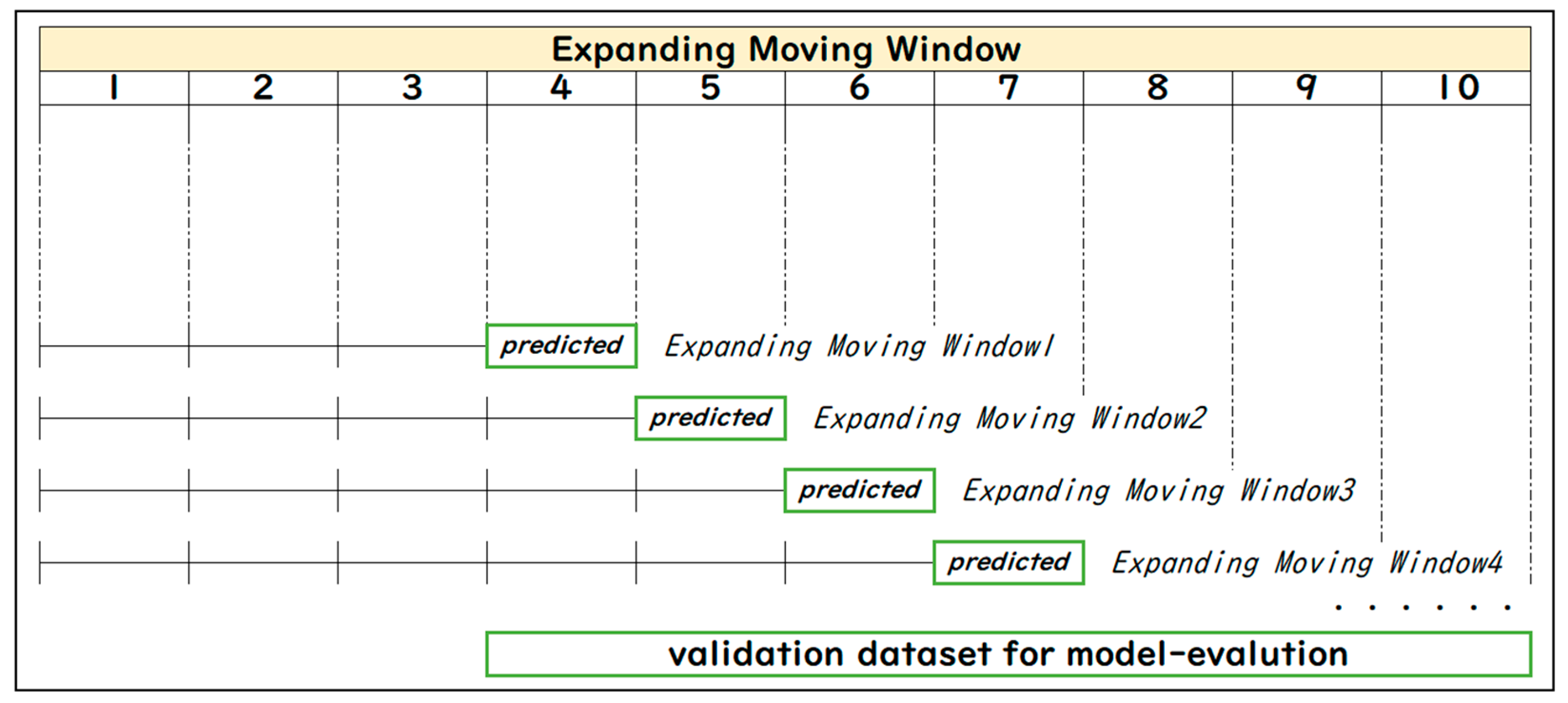
This study employs two patterns of moving window techniques to predict one-period-ahead, aiming to investigate whether there is a difference in prediction performance when excluding historical data. One pattern is the fixed-length moving window (FMW) technique, and the other is the expanding-length moving window (EMW) technique.
The moving window statistics proceed iteratively with the prediction, extending or shifting the size of EMW or FMW by one time step in each iteration.
Figure 4 illustrates the mechanism of EMW, while
Figure 5 depicts the mechanism of FMW.
In terms of the expanding-length window, the initial window size is set to 3363, which is the same as the length of the validation data (there are 3957 observations from 3 February 2003 to 16 December 2020). When iterating the model fitting, the window size increases by one period. For example, the first window spans from 3 February 2003 to 16 July 2017, and is used to estimate 17 July 2017. The framework utilizes the dataset from period 1 to 3363 to train the model, then uses the trained model to forecast period 3364, and incorporates the extended training dataset from period 1 to 3364 to retrain the model. The updated model is then used to predict period 3365. This process is iterated until the last period of the time series. The expanding moving window technique is also employed in the model evaluation as walk-forward testing (
Baranochnikov and Ślepaczuk 2022).
In terms of the fixed-length window, the window size is determined to be 3363. For instance, the first window spans from 3 February 2003 to 16 July 2017, and is used to estimate 17 July 2017. The model uses the dataset from period 1 to 3363 to train the model and utilizes this trained model to forecast period 3364. Then, the dataset from period 2 to 3364 is used to train the model, and the updated model is used to predict period 3365. This process is iterated until the last period of the time series.
3.2.2. Random Forest (RF)
The RF approach, introduced by
Breiman (
2001), is an ensemble machine learning method that incorporates multiple decision trees to improve prediction performance. By extending each tree from randomly selected features and building them from the primal sample, the RF method addresses the overfitting problem that can arise when adding more trees to the forest. This approach enhances prediction accuracy.
To maximize the forecasting performance of our model, we conducted a meticulous parameter-tuning process. We optimized several variables to achieve optimal results in our forecasting endeavor. The variables that underwent optimization included n_estimators (with values of 100, 200, 300, 400, and 500), max_depth (with values of 1, 3, 10, 20, 30, 40, and 50), bootstrap (with options of True and False), and min_samples_leaf (ranging from 1 to 10). After a thorough evaluation based on error metrics, we selected the following parameter values: n_estimators (300), max_depth (20), bootstrap (True), and min_samples_leaf (3). These parameter values were found to yield the best performance in our model, ensuring accurate and reliable forecasting outcomes.
3.2.3. Extreme Gradient Boosting (XGBoost)
XGBoost, an algorithm proposed by
Chen and Guestrin (
2016), is an ensemble machine learning model that enhances gradient boosting techniques (
Friedman 2001). It employs an optimized platform for gradient boosting, leveraging parallel processing, tree pruning, and hardware optimization. XGBoost offers a variety of objective functions, including classification and regression, and combines weaker and simpler learner estimates (such as regression trees) to improve prediction accuracy. The model minimizes a subjective loss function through a penalty term for model complexity (i.e., regression tree functions) and a convex loss function. Iterative learning involves creating new trees and merging them with existing trees.
To enhance the predictive performance of our model, we conducted a meticulous parameter-tuning process. We optimized several variables to achieve optimal results in our forecasting endeavor. The variables that underwent optimization included n_estimators (ranging from 100 to 1000 in increments of 100), max_depth (with values of 1, 3, 5, and 10), learning_rate (with values of 0.001 and 0.01), and gamma (with values of 0, 0.001, and 0.01). Subsequently, based on the performance evaluation using error metrics, we selected the following parameter values: n_estimators (1000), max_depth (3), learning_rate (0.01), and gamma (0.01).
3.2.4. Long Short-Term Memory (LSTM)
The LSTM algorithm was first introduced by
Hochreiter and Schmidhuber (
1997). As a prominent model in deep learning, LSTM exhibits an external loop structure similar to that of RNN and an internal recurrent structure consisting of memory cells. Each memory cell possesses self-connected recurrent weights that interact with three types of gates, ensuring the preservation of signals over multiple time steps without suffering from exploding or vanishing gradients. Similar to RNN, LSTM can utilize more data at each time step, resembling the memory capacity of the LSTM unit. The network utilizes these gates to effectively manage the retention and forgetting of information for subsequent iterations.
To achieve optimal forecasting outcomes, we meticulously tuned the hyperparameters of our model. Various variables underwent optimization, including batch size (ranging from 10 to 200), number of epochs (ranging from 10 to 300), optimization technique (SGD, Adam, RMSprop), learning rate (0.001, 0.01, 0.1), dropout rate (ranging from 0.0 to 0.9), neuron activation function (relu, sigmoid), number of layers (ranging from 1 to 5), and number of neurons (16, 32, 46, 64, 128). During the training of the neural networks, we employed the traditional mean squared error (MSE) loss function, as utilized by
Cao et al. (
2019),
Chimmula and Zhang (
2020), and
Livieris et al. (
2020). This loss function is widely recognized and commonly used in the field. Following a comprehensive evaluation process, we selected the following parameter values that exhibited superior performance: a batch size of 15, 150 epochs, the Adam optimization technique, a learning rate of 0.001, no dropout (dropout rate of 0.0), relu activation function, 3 layers, and 46 neurons. These parameter values were determined to produce the most accurate and reliable forecasting results in our model.
3.2.5. AutoRegressive Integrated Moving Average (ARIMA)
ARIMA was developed in the 1970s by
Box and Jenkins (
1968) with the aim of mathematically characterizing variations in time series. Non-stationary data need to be differenced until stationarity is achieved, as ARIMA specifically works with stationary data. In ARIMA (p, d, q), where p represents the autoregressive terms, d represents the differencing order, and q represents the lagged errors, the best values for p, d, and q are determined using the Akaike information criterion to fit the data.
In this study, the selection of optimal (p, d, q) values for time series analysis is performed using the auto_arima function in Python. The auto_arima function employs a stepwise search method to minimize the Akaike Information Criteria (AIC). To ensure model parsimony, the maximum values for p and q are set to be less than 5. The determination of the optimal differencing parameter, d, is achieved through the application of the Augmented Dickey-Fuller test.
3.2.6. Wavelet-ARIMA-LSTM (Wavelet-ARIMA-RF/Wavelet-ARIMA-XGB)
The wavelet transform was first introduced by French scientist J. Morlet in 1974 (
Morlet et al. 1982). Wavelet decomposition has been widely utilized as a preprocessing approach in various fields such as engineering, time series analysis, and medicine. By applying wavelet decomposition, time series data can be separated into approximation and detail components. In this study, we employ discrete wavelet decomposition (DWD) to decompose the gold futures prices and the euro exchange rate into multiple approximation and detail component series. Unlike previous research, we simplify the analysis by using the decomposed approximation series for forecasting one-period-ahead values using the ARIMA model. We then calculate the residuals and apply the LSTM model to predict the one-period-ahead residuals, and finally combine them.
In summary, the DWD technique is employed to decompose the price time series into linear approximation components and nonlinear residual components. The linear components are predicted using the ARIMA model, while the nonlinear parts are independently forecasted using the LSTM model, taking into account the intrinsic characteristics of these models.
Similarly, in the case of wavelet-ARIMA-RF and wavelet-ARIMA-XGB, the random forest model and extreme gradient boosting are applied, respectively, to predict the nonlinear components.
3.2.7. Seasonal-Decomposition-ARIMA-LSTM
Furthermore, we employed another preprocessing technique, known as traditional seasonal decomposition, for the time series models of gold futures prices and the euro exchange rate. According to the traditional concept of time series decomposition, a series is considered as a composite of level, trend, seasonality, and noise components. In this study, we regard the level, trend, and seasonality components as systematic components since they exhibit consistency or recurrence and can be described and modeled. Conversely, we classify the noise component as non-systematic due to its random variation nature. Diverging from previous research, we utilize the decomposed systematic components, including the trend series and seasonality series, to apply the ARIMA model for forecasting one-period-ahead values. Subsequently, we employ the decomposed non-systematic noise components to apply the LSTM model for predicting one-period-ahead noise, and ultimately aggregate these predicted values.
In summary, the traditional seasonal decomposition method is utilized to decompose the price time series into linear systematic components and nonlinear non-systematic components. The linear components are then forecasted using the ARIMA model, while the nonlinear components are separately predicted using the LSTM model.
3.3. Model Evaluation Measures
3.3.1. Root Mean Squared Error (RMSE)
The discrepancy between the expected and actual values is typically measured using the RMSE. The RMSE is typically computed as follows:
where
is the number of non-missing data points,
is the actual observation time series, and
is the estimated time series.
3.3.2. Mean Absolute Percentage Error (MAPE)
The accuracy of forecasting models is frequently assessed statistically using the mean absolute percentage error (MAPE). MAPE can be calculated as the average absolute percent error for each time period minus actual values divided by actual values. Generally speaking, the following equation defines MAPE:
where
variable,
number of non-missing data points,
actual observation time series,
estimated time series.
This paper defined the MAPE accuracy (%) by .
3.3.3. Mean Absolute Error (MAE)
The mean absolute error (MAE) is frequently used as a statistical measure of the average magnitude of the errors in a predicted dataset without considering their direction. It is the average over the test sample of the absolute differences between prediction and actual observation, where all individual differences have equal weight. Generally, MAE is defined by the following equation:
where
variable,
number of non-missing data points,
actual observation time series,
estimated time series.
3.3.4. Modified Diebold–Mariano Test
The DM test was originally introduced by
Diebold and Mariano (
1995). In empirical analyses, when there are two or more time series forecasting models, it is often a challenge to predict which model is more accurate or whether they are equally suitable. This test identifies whether the null hypothesis (i.e., that the competing model holds equivalent forecasting power as the base model) is statistically true. Assuming that the actual values
, two forecasts
,
, and forecast error
are as follows:
where
denotes the forecast error and the loss function,
, which is defined by the following function:
Then, the loss differential
is expressed as follows:
Correspondingly, the statistic for the DM test is expressed using the following formula:
where
denote the mean loss differential, the variation of
, and the number of data points, respectively.
The null hypothesis is , meaning that the two forecast models hold equivalent forecasting performance. Meanwhile, the alternative hypothesis is , which represents the difference in accuracy between these two forecasts. Under the null hypothesis, the statistics for the DM test are asymptotically normally distributed. The null hypothesis would be rejected when .
Harvey et al. (
1997) proposed a modified DM test. They suggested that the modified DM test is more suitable when using a small sample. The statistic for the modified DM test is expressed as follows:
where
represents the horizon and
refers to the original
statistic. Here, we predicted one-period-ahead; hence,
h = 1; hence,
Concerning how to interpret the DM test statistic results, since we set as the target model, as the base model, the numerator is (target-base), therefore, if the DM test statistic is negative, that means the target model has a smaller variance than the base model; hence, the prediction performance of the target model is better than the base model. The p-value denotes the significance of this statistic.
4. Results
4.1. Empirical Results
4.1.1. Prediction Results of SI Dataset and Large Dataset
Firstly, this subsection presents the prediction performance results of the sentiment dataset and the large dataset to verify whether the sentiment dataset could replace the large dataset when predicting commodity gold prices and the euro foreign exchange rate.
Table 2 displays the prediction outcomes for gold futures prices utilizing the sentiment indicator dataset, while
Table 3 presents the prediction results for gold futures prices employing the large dataset. Likewise,
Table 4 lists the prediction results for the euro foreign exchange rate based on the sentiment indicator dataset, and
Table 5 showcases the prediction results for the euro foreign exchange rate utilizing the large dataset. Overall, the prediction results indicate that the sentiment indicator dataset generally exhibits better forecasting performance than the large dataset. When comparing the performance metrics, namely RMSE, MAPE, and MSE, between the two datasets, it becomes evident that the fixed moving window LSTM approach using the SI dataset outperforms the alternative dataset and models considered. This finding suggests that combining the sentiment indicator with the moving window LSTM machine learning model yields the best results for predicting gold futures prices and euro exchange rates. These results align with the outcomes of previous studies by
Plakandaras et al. (
2015),
Nwosu et al. (
2021), and
Dunis and Williams (
2002), which suggest that neural network models or their proposed approaches, particularly when combined with neural networks, offer more accurate forecasts compared to other models. Furthermore, these results provide additional evidence supporting the superiority of the LSTM model’s complex loop structure. Turning to the forecasting results using the large dataset, the moving window RF results demonstrate the best performance. This may be attributed to the use of a large indicator dataset, which allows the RF classifier to effectively enhance the predictive power. Although our study employs a different data source for sentiment analysis compared to previous research (
Naeem et al. 2021), our empirical results broadly align with the findings of
Li et al. (
2016) and
Naeem et al. (
2021) in terms of predicting gold futures and euro exchange rates, thus indicating that the sentiment dataset can serve as a viable substitute for the large dataset.
4.1.2. Prediction Results of ARIMA Model
However, when comparing with the classical statistical model, ARIMA, whether the conclusion holds robustness needs to be investigated. Therefore, we conducted the simple prediction by ARIMA, and the lags were chosen using the Akaike Information Criteria (AIC). The forecasting results are presented in
Table 6.
Based on the above results, we are pleasantly surprised by the effectiveness of the powerful yet simple statistical model, ARIMA, in predicting time series. This finding aligns with the research reported by
He (
2018). However, it contradicts the studies conducted by
Siami-Namini et al. (
2018) and
Siami-Namini et al. (
2019). These results suggest that simplicity may be the key when it comes to designing prediction models for time series, despite the prevalence of complex models and fancy datasets. In contrast to the findings of
Nwosu et al. (
2021) and
Dunis and Williams (
2002), our results indicate that it is worth considering the use of simple traditional models in the design of prediction models.
4.1.3. Prediction Results of Proposed Approaches
However, it is worth noting that machine learning and deep learning models have been extensively validated in numerous studies for their superior effectiveness and accuracy in predicting time series compared to ARIMA models. Therefore, it is necessary to further verify the robustness of the simple statistical model, ARIMA. Inspired by
Abdulrahman et al. (
2021) and others, we propose a triple combination of wavelet-ARIMA-LSTM, wavelet-ARIMA-RF, and wavelet-ARIMA-XGB models, as well as the seasonal-decomposition-ARIMA-LSTM approach, to investigate this objective. The prediction results are summarized in
Table 7 and
Table 8.
Based on the results presented in
Table 7 and
Table 8,
Figure 6 and
Figure 7, our proposed triple-combination approach demonstrates superior prediction accuracy compared to individual ARIMA, machine learning, and deep learning approaches. This suggests that by decomposing time series into linear and nonlinear components and combining classical statistical models with machine learning approaches, we achieve more precise predictions. However, the best performing approach for both object time series, namely gold futures prices and the euro foreign exchange rate, is the SeasonalDecomposition_ARIMA_LSTM model. It is followed by Wavelet_ARIMA_XGB and Wavelet_ARIMA_RF. This finding suggests that the systematic and non-systematic decomposition combined with the ARIMA and LSTM models for predicting commodity prices and foreign exchange rates is preferable. These results align with previous studies (
Chang et al. 2019;
Chen and Wang 2019;
Liu et al. 2018;
Ma et al. 2019;
Moustafa and Khodairy 2023), further supporting the effectiveness of the integrated multiple-model approach in prediction. Our empirical forecasting results provide additional evidence that the multiple-model integrated approach performs better in prediction.
In summary, first, the combination of the sentiment indicator with the fixed moving window LSTM machine learning model produces the best prediction results compared to the large dataset. This result demonstrates that sentiment indicators obtained through sentiment analysis outperform the large dataset in terms of prediction ability and can be utilized as a better alternative independent predictor. Second, based on the prediction results, the traditional and classical ARIMA model surprisingly outperforms both the sentiment indicator dataset and the large dataset combined with machine learning techniques. Finally, our proposed triple-combination techniques are superior to both machine learning models and the traditional statistical ARIMA model in terms of commodity price and foreign exchange rate prediction performance. The top three performing forecasting methods are the seasonal-decomposition_ARIMA_LSTM, the wavelet_ARIMA_XGB, and the wavelet_ARIMA_RF. In the first step, these approaches decompose the data into linear and nonlinear components by adopting seasonal decomposition or wavelet transformation. In the second step, they use the ARIMA model to predict the linear part and machine learning or deep learning models to predict the nonlinear part.
4.2. Model Evaluation Results
4.2.1. Walk-Forward Testing Results
In this study, we employ the walk-forward testing method as the chosen back-testing technique to validate the effectiveness of the proposed triple-combination approaches. To evaluate the performance of these models, we adopt an expanding moving window approach, focusing on the last 50 observations. The testing procedure involves conducting separate walk-forward tests on each decomposition component, followed by aggregating the results and comparing the error metrics against those obtained from the ARIMA model.
As we present in
Table 9 and
Table 10, the walk-forward testing results for gold futures prices and euro foreign exchange provide robust estimations for evaluating the effectiveness of our proposed triple-combination approaches. These results offer valuable insights into the performance and reliability of the models in predicting the respective market dynamics.
4.2.2. Diebold–Mariano Test Results
The Diebold–Mariano test is conducted to assess the predictive superiority of the triple-combination approaches compared to the ARIMA models. We present the results of this test in
Table 10 and
Table 11, offering insights into the relative performance of the proposed approaches. The DM test results for both gold futures prices and euro foreign exchange rates are analyzed.
From the results presented in
Table 11 and
Table 12, it is noteworthy that the proposed triple-combination approaches demonstrate a significant outperformance over the classical statistical model, the ARIMA model.
5. Conclusions and Policy Implications
As highlighted by
Naeem et al. (
2021) and
Li et al. (
2016), the rapid advancement of the Internet and big data technology has led to an abundance of online data, including textual data from sources such as Twitter and news releases, which can help to identify influential factors in specific markets. Motivated by this, our study aims to examine whether the sentiment indicator dataset obtained through sentiment analysis of unstructured online news headlines can serve as a substitute for the large dataset comprising various indicators in predicting commodity prices and foreign exchange rates.
In our empirical analysis, we employ sentiment analysis using the Python natural language processing library to process news headlines from ABC, which consists of 1,226,258 news headlines, to derive a sentiment indicator. Additionally, we collect 30 additional indicators to construct the large dataset. Subsequently, we utilize this sentiment indicator in conjunction with moving window machine learning and deep learning models, namely RF, XGBoost, and LSTM, to forecast commodity gold futures prices and the euro exchange rate. Alongside comparing the prediction performance of the datasets, we also conduct a prediction comparison between the classical statistical model, ARIMA, and time-varying parameter machine learning models.
Based on the results of the model comparisons, we cannot conclude that sentiment indicators combined with machine learning outperform the ARIMA model. However, from an alternative perspective, we propose triple-combination approaches that involve decomposing the time series data into linear and nonlinear components and subsequently forecasting the linear component using the robust statistical model, ARIMA, and the nonlinear component using machine learning models such as LSTM, XGB, and RF. This research sheds light on the issue of comparing the out-of-sample superiority of our proposed triple-combination approaches for foreign exchange rate prediction with the traditional powerful statistical model, ARIMA. Furthermore, we conduct walk-forward testing to validate the triple-combination approaches and employ the modified Diebold–Mariano test statistic to investigate statistically significant differences between the proposed approach and the ARIMA model.
The study’s primary conclusions are as follows: Firstly, the combination of the sentiment indicator with the moving window LSTM machine learning model demonstrates the best forecasting performance. These findings align with previous studies conducted by
Plakandaras et al. (
2015),
Nwosu et al. (
2021), and
Dunis and Williams (
2002). Secondly, the sentiment indicator dataset used by deep learning and moving window machine learning models does not surpass the classical ARIMA model, consistent with the findings reported by
He (
2018). This result contradicts the studies conducted by
Siami-Namini et al. (
2018) and
Siami-Namini et al. (
2019). Thirdly, the proposed triple-combination methods, which expand upon and derive from the approaches of
Chang et al. (
2019),
Chen and Wang (
2019),
Liu et al. (
2018),
Ma et al. (
2019), and
Moustafa and Khodairy (
2023), exhibit superior performance in predicting commodity prices and foreign exchange rates compared to both machine learning models and the ARIMA model. The seasonal-decomposition ARIMA-LSTM, wavelet-ARIMA-XGB, and wavelet-ARIMA-RF demonstrate the top three forecasting performances based on error metrics, walk-forward testing results, and Diebold–Mariano test results. In the first step, the data are decomposed into linear and non-linear components using wavelet transformation or seasonal decomposition. In the second step, the linear component is predicted using ARIMA, while the non-linear component is predicted using machine learning or deep learning models. Lastly, in addition to the aforementioned findings, the comparison of results between the sentiment indicator dataset and the large dataset indicate that sentiment indicators obtained through sentiment analysis possess superior forecasting capabilities compared to the large dataset consisting of various indicators. Consequently, they can be utilized as better alternative predictors. Our empirical results generally align with the findings of
Li et al. (
2016) and
Naeem et al. (
2021) in terms of predicting gold futures and euro exchange rates, further highlighting the potential of the sentiment dataset to enhance forecasting in time series prediction.
To the best of our knowledge, this study presents a pioneering investigation into the potential of sentiment indicators as a substitute for extensive datasets in forecasting commodity prices and foreign exchange rates. The novelty lies in proposing a novel integration of machine learning models, statistical models, and data decomposition techniques to enhance price predictions in these markets. Importantly, the results validate the superior accuracy of the proposed triple-combination approach compared to individual models. Furthermore, these findings offer valuable insights for investors and policymakers, providing them with fresh perspectives, predictive tools, and alternative forecasting approaches.
For investors, the research offers fresh perspectives on forecasting commodity prices and foreign exchange rates. It introduces new predictive tools and alternative approaches that enhance their decision-making processes and potentially lead to more accurate forecasts. Additionally, precise prediction of gold prices and euro exchange rates is crucial for informing hedging strategies aimed at mitigating risks arising from currency fluctuations.
For policymakers, these findings play a vital role in making informed investment decisions. Gold is widely utilized as a means to hedge against inflation and market volatility, and fluctuations in the euro exchange rate have a substantial impact on the costs and risks associated with international transactions as the second most traded currency globally. Moreover, improving the accuracy of gold price predictions is crucial for central banks that maintain gold reserves as a safeguard against currency fluctuations and as a store of value. Given that the euro is a major reserve currency used in international transactions and investments, precise prediction of euro exchange rates can bolster financial stability. Furthermore, gold prices and euro exchange rates are closely intertwined with the international economy and play a pivotal role in informing government policy decisions regarding trade, monetary policy, and capital flows. Therefore, our findings contribute to economic forecasting, empowering policymakers and investors to leverage these predictions for informed decision making, ensuring they are well-prepared to navigate and respond to evolving economic conditions.
Despite these findings, this study has its limitations. Since we only employ RF, XGB, and LSTM methods to compare forecasts with the ARIMA model, we cannot conclusively determine that ARIMA is superior to other machine learning and deep learning models. Further verification is necessary to address this point. Additionally, there are numerous other data decomposition methods that require testing to validate the conclusions.
In future research, it is recommended to explore alternative data decomposition methods, as well as additional machine learning and deep learning techniques, to expand the investigation to major commodity prices and currency exchange rates. This will help validate the rationality and robustness of the proposed approaches’ superiority. Furthermore, considering the potential of the sentiment indicator as a promising alternative dataset, empirical testing is planned to assess whether incorporating the proposed approaches with the additional sentiment indicator can further enhance the forecasting accuracy for commodity prices and foreign exchange rates.


