Article

Dynamic Relationship between Volatility Risk Premia of Stock and Oil Returns

Graduate School of Business Administration, Hitotsubashi University, 2-1-2 Hitotsubashi, Chiyoda-ku, Tokyo 101-8439, Japan
*
Author to whom correspondence should be addressed.
J. Risk Financial Manag. 2023, 16(3), 173; https://doi.org/10.3390/jrfm16030173
Submission received: 27 December 2022 / Revised: 17 February 2023 / Accepted: 27 February 2023 / Published: 5 March 2023
(This article belongs to the Special Issue Commodity Market Finance)

Abstract

:
This study investigates the relationship between the volatility risk premia (VRP) of stock and oil returns. Using daily data on VRP from 10 May 2007 to 16 May 2017, VAR analyses on the stock and oil VRP are conducted, and it is found that the effects of the stock VRP on the oil VRP are limited and, if any, short-lived. In contrast, the VRP of oil has significantly positive and long-lasting effects on the stock VRP after the financial crisis. These results suggest that investors’ sentiments (measured by VRP) are transmitted from the oil to the stock market over time, but not vice versa. This is unexpected because the financialization of commodities means a massive increase in investment in commodities by investors in the traditional stock and bond markets; hence, the direction of effects is thought to be from the stock to the commodity market.

1. Introduction

The volatility risk premium (VRP), defined as the difference between implied and realized volatilities, has been found to have predictive power for returns in many different assets. For example, as pioneering research on this topic, Bollerslev et al. (2009a) revealed that VRP has predictive power for U.S. monthly aggregated stock returns, and Bollerslev et al. (2009b) also found the predictive power of the VRP in the monthly stock index returns of many other developed countries.
The VRP represents the risk premium for future volatility variations. Thus, it may be regarded as investor sentiment (i.e., aversion to future uncertainty), and the predictability of VRP is thought to be due to investor sentiment: when investor sentiment worsens (resp. improves), stock prices are discounted by a higher (resp. lower) premium, resulting in higher (resp. lower) future returns.
Following this intuition, the scope of the analysis is extended to assets other than stocks. Indeed, Della Corte et al. (2016) and Londono and Zhou (2016) confirmed the predictive power of VRP in monthly exchange rates. Furthermore, Ornelas and Mauad (2019) investigated the predictive power of different assets’ VRP such as commodities currencies, stocks, bonds, gold, and oil, on the monthly returns.
Given the extant research on VRP’s return predictability of different assets, one simple but unexplored question is how the VRP of different assets are correlated. This question is meaningful because the dynamic relation of the VRP between different assets is interpreted to show how investors’ sentiments on different assets transmit to each other over time. Moreover, it is especially important between the VRP of stocks and commodities because the recent financialization of commodities, that is the massive increase in investment in commodities by investors in the traditional stock and bond markets, is thought to increase the influence of the stock market on commodity markets. Thus, this study investigates the dynamic relationship between the VRP of stocks and oil using their daily returns.
Note that this focus is unique compared to previous studies. Indeed, many extant studies have investigated the relationship among implied volatilities of stock, oil, gold, and exchange rate. However, they are not related to VRP. For example, Robe and Wallen (2016) analyzed the determinants of oil implied volatility using weekly data and investigated the relationship between oil implied volatility and stock implied volatility. Christoffersen and Pan (2018) investigated the effect of oil implied volatility on stock returns and analyzed the relationship between oil implied volatility and stock implied volatility. Liu et al. (2013) conducted a VECM analysis on the relation among daily implied volatilities of stock, oil, gold, and exchange rates. Dutta et al. (2019) analyzed co-integration and nonlinear causality among the implied volatilities of crude oil, gold, silver and goldminers by a non-linear ARDL model. Bouri et al. (2020) studied the dynamic spillovers among the implied volatilities of the S&P 500 and five large US stocks based on Diebold and Yilmaz’s (2014) connectedness model. Iqbal et al. (2022) analyzed spillover among implied volatilities of international stock and commodity indices by a quantile VAR model. Moreover, Gagnon et al. (2015), Zhang et al. (2022), and Bouri et al. (2023) analyzed the relationship among implied higher order moments of stock indices and commodities.
Given those previous studies, the main goal of this study is to investigate the dynamic relation of daily VRP, not implied volatilities, between stocks and oil, and to show how investors’ sentiments, represented by VRP, on different assets transmit each other over time. A paper closely related to this is Hattori et al. (2021), who conducted a VAR analysis on the relationship among daily stock VRP of advanced and emerging market economies. Our study differs in that it investigates the dynamic relationship of VRP between stock and oil and analyzes the spillover of investors’ sentiments, not within stock markets, but between stock and commodity markets. To the best of our knowledge, this is the first study to address this issue.
Following the method of Bollerslev et al. (2009a), we calculate the daily VRP of stock as the difference between the VIX published by the Chicago Board of Trade (CBOE), which measures the 30-day implied volatility of S&P 500 stock index options, and the daily realized volatility of the S&P 500 stock index provided by the Oxford-Man Institute of Quantitative Finance. To obtain the daily VRP of oil, we use the OVX published by the CBOE, which measures the 30-day implied volatility of crude oil prices by applying the CBOE Volatility Index methodology to options on the United States Oil Fund (USO). Because we do not have high-frequency data of the USO prices and hence cannot directly calculate its daily realized volatility, we estimate the daily realized volatility of oil by applying a stochastic volatility model to its returns (see Appendix A).
Using the daily VRP of stock and oil returns obtained between 10 May 2007 and 16 May 2017, we conduct a VAR analysis of the VRP and obtain the following results: During the whole period and all sub-periods, both VRP are stationary and their correlations are approximately 0.2 to 0.3, except in the pre-crisis period (between 10 May 2007 and 30 May 2008), where the correlation is less than 0.1.
For the whole period, most of the variations in the VRP are explained by their own shocks, which may seem against what we expect from the financialization of commodities because financialization is regarded as strengthening the relationship between stock and oil. Meanwhile, the shocks in both the VRP of stock and oil have small but significant positive effects on each other for most of the following 20 trading days after the shock. This is in contrast with the results shown by Liu et al. (2013) on the relationships among the implied volatilities of stock, oil, gold, and euro/dollar exchange rates, in which all implied volatilities have significant, but only temporary (i.e., just on the 1st trading day after the shock) effects on each other.
However, such relationships depend on the economic situation, and the economic situation surrounding stock and oil has been clearly changing. Thus, we conduct a VAR analysis on the following sub-periods: Period 1 from 10 May 2007 to 31 May 2008 (pre-crisis period), Period 2 from 1 June 2008 to 30 June 2009 (crisis outbreak period), Period 3 from 1 July 2009 to 31 July 2012 (post-crisis recovery period I), Period 4 from 1 August 2012 to 30 September 2014 (post-crisis recovery period II), and Period 5 from 1 October 2014 to 16 May 2017 (plunging oil price period). Interestingly, the analysis of these sub-periods reveals a different picture of the dynamic relationship between stock and oil VRP from that of the entire period.
In the pre-crisis period (Period 1), we find that there is little or no relation between the VRP of stock and oil: a small correlation of less than 0.1, no Granger causality between the stock and oil VRP, or no significant effects on each other in impulse response functions and little effect on variance decomposition. Again, this may seem somewhat against the view of the financialization of commodities because the financialization effect, that is the rise of correlations among the returns of stock and commodities, emerged after the 2000s (Tang and Xiong 2012; Silvennoinen and Thorp 2013; Ohashi and Okimoto 2016).
In the crisis outbreak period (Period 2), the correlation between the VRP of stock and oil is 0.27. The stock VRP does not Granger cause an oil VRP. There are no significant effects of the stock VRP on the oil VRP in either the impulse response functions or variance decomposition. In contrast, the oil VRP Granger causes the stock VRP, has significantly positive, though small, effects on the stock VRP in impulse response and explains 8% of the variation in the stock VRP.
In post-crisis recovery period I (Period 3), the correlation increases to 0.34. Both the stock and oil VRP Granger cause each other. Both have small but significantly positive effects on each other in the impulse response functions and variance decomposition. However, their effects have quite different patterns: The VRP of oil has significantly positive and long-lasting effects (after the 2nd trading day of the shock), whereas the VRP of stock has significantly positive but only temporary effects (just up to the 2nd trading day) on that of oil.
In post-crisis recovery period II (Period 4), the correlation decreases to 0.21. The Granger causality from stock to oil disappears, while the VRP of oil Granger causes that of the stock. The effects of the oil VRP on the stock VRP remain significant and long-lasting, similar to those in Period 3, but the effects of the stock VRP on the oil VRP disappear.
Finally, in the plunging oil price period (Period 5), the correlation is 0.22. Both Granger cause one another. The effects of the VRP of stock on that of oil are back to significantly positive, but only temporarily on the 1st trading day after the shock, while the effects of the oil VRP on the stock VRP remain significantly positive up to the 8th trading day after the shock.
In summary, the dynamic relationship between the VRP of stock and oil depends on the economic situation, and contrary to the results for the whole period, it is revealed that the VRP of oil has significantly positive and long-lasting effects on that of stock in all sub-periods after the outbreak of the financial crisis, while the effects of the stock VRP on the oil VRP are limited and, if any, much more short-lived. That is, although small, investors’ sentiments are transmitted from the oil market to the stock market over time, but not vice versa. This relationship between oil and stock VRP is an unexplored point in the extant literature and is rather unexpected because the financialization of commodities, that is the massive increase in investment in commodities by investors in the traditional stock and bond markets, is thought to have effects from the stock to the commodity market.1
The remainder of this paper is organized as follows. Section 2 explains VRP. Section 3 discusses the construction and properties of the data used in the study. Section 4 describes the model selection. Section 5 presents our main empirical results. Section 6 discusses the robustness of the analysis. Section 7 provides the conclusion.

2. Volatility Risk Premium (VRP)

Let t denote the current date. Denote by σ t + T the volatility of an asset return at date t + T . A volatility swap that exchanges on date t + T the payoff σ t + T and the payment x t , which is contracted at date t , enables its holder/investor to hedge on date t the risk of volatility variation in the future date t + T .2 A simple no-arbitrage argument shows that x t = E t Q [ σ t + T ] , where Q is the risk-neutral probability. Hence, the amount that the swap investor receives on date t + T is equal to σ t + T E t Q [ σ t + T ] .
If σ t + T is on average less than E t Q [ σ t + T ] , that is, E t P [ σ t + T ] E t Q [ σ t + T ] < 0 where P is the original probability, it means that the swap holder is willing to pay E t Q [ σ t + T ] , which is more than the expected payoff E t P [ σ t + T ] , to hedge the volatility risk in the future. In this sense, E t Q [ σ t + T ] E t P [ σ t + T ] represents the premium the swap investor is willing to pay to hedge the variation risk of future volatility. Thus, E t Q [ σ t + T ] E t P [ σ t + T ] is the volatility risk premium (VRP).
As visible, the larger the VRP is, the more averse the investor is about the variation in future volatility. In this sense, the VRP is sometimes interpreted as indicating investor sentiment on future asset returns.

3. Data

In the empirical analysis, we estimate the risk-neutral expected future volatility E t Q [ σ t + T ] and the expected future volatility E t P [ σ t + T ] to calculate the VRP. The former can be estimated from option prices, and hence is called the (option) implied volatility (IV). However, the latter estimation is not immediate. Hence, following the method of Bollerslev et al. (2009a), we approximate the expected future volatility by the realized volatility (RV) and obtain VRP as the difference between IV and RV, that is, VRP     IV RV .3
More precisely, we calculate the daily VRP of stock ( VRP sp ) as the difference between the VIX published by the Chicago Board of Trade (CBOE),4 which measures the 30-day implied volatility of S&P 500 stock index options, and the daily realized volatility of the S&P 500 stock index provided by the Oxford-Man Institute of Quantitative Finance, which is calculated from 5 min returns of the index.5 As noted above, while the former is risk-neutral expected future volatility, the latter is not expected future volatility, but daily realized volatility. Thus, by this choice of variable, we assume that the daily realized volatility of the Oxford-Man Institute approximates the expected future volatility of the stock well.
To obtain the daily VRP of oil ( VRP oil ), we use the OVX published by the CBOE,6 which measures the 30-day implied volatility (i.e., the risk-neutral expected future volatility) of crude oil prices by applying the CBOE Volatility Index methodology to options on the United States Oil Fund (USO). Because we do not have high-frequency data of the USO returns to calculate its daily realized volatility, we estimate the daily realized volatility of oil by applying a stochastic volatility model to its returns.7 Then, we obtain the daily VRP of oil (VRP_oil) as the difference between the OVX and the daily realized volatility of oil. Again, by doing so, we assume that the daily realized volatility of oil approximates the expected future volatility of oil.
As the CBOE publishes OVX data after the middle of 2007, we use the daily VRP of stock and oil returns from 10 May 2007 to 16 May 2017. In this period, however, global financial markets and the world economy went through several different phases such as the global financial crisis around the collapse of Lehman Brothers, the recovery from the financial crisis, and the plunge of oil prices, all of which may affect the relationship between stock and oil prices.
For example, this is visible from graphs of the daily indices of stock (S&P 500) and oil (USO) in Figure 1 where index_sp represents S&P 500 price and index_oil represents USO price multiplied by 50, the vertical axis is measured in U.S. dollars, and time in the horizontal axis represents the date where time 1 corresponds to 10 May 2007, time 500 to 13 May 2009, time 1000 to 6 May 2011, time 1500 to 3 May 2013, time 2000 to 29 April 2015, and time 2500 to 24 April 2017, respectively.
Thus, while we use the daily VRP of stock and oil returns between 10 May 2007 and 16 May 2017 to reflect the changes in economic phases, we divide the entire period into five sub-periods and investigate whether and how the VRP of stock and oil are related in each period. The sub-periods are listed in Table 1.
We select those periods based partly on Liu et al. (2013), who investigated the dynamic relation among the implied volatilities of stock (VIX), oil (OVX), euro/dollar exchange rate (EVZ), and gold (GVZ) between 3 June 2008 and 20 July 2012. Indeed, Period 2, which is the crisis outbreak period centered on the collapse of Lehman Brothers on 15 September 2008, roughly corresponds to Liu et al.’s (2013) crisis outbreak period, and Period 3, post-crisis recovery period I, corresponds to their post-crisis recovery period so that we can for those periods compare the interaction among implied volatilities shown by Liu et al. (2013) with that of VRP analyzed by this paper. Period 1 is before the outbreak of the global financial crisis. Period 4 is the post-crisis recovery period beyond Liu et al.’s (2013) post-crisis recovery period. Finally, Period 5 is the period of the oil price plunge after the summer of 2014, which may change the relationship between stock and oil VRP.
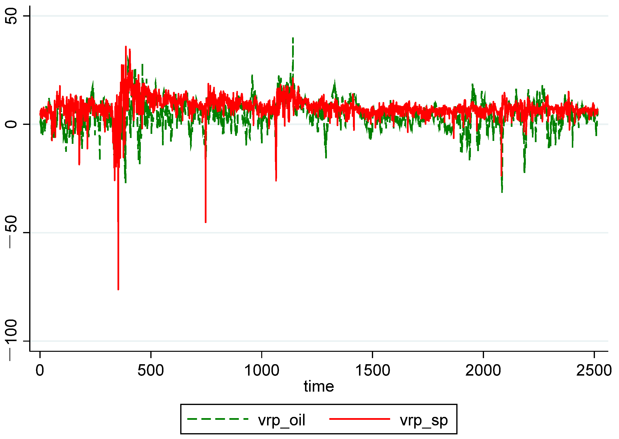
Figure 2 shows the relationship between VRP sp and VRP oil from 10 May 2007 to 16 May 2017. Here, both stock and oil VRP appear volatile especially during the crisis outbreak period (Period 2) and are calming in the post-crisis recovery periods (Periods 3 and 4). However, the oil VRP then becomes slightly volatile in accordance with the recent plunging oil prices (in Period 5).
The descriptive statistics of the daily VRP of stock and oil are given in Table 2. It confirms our observation about their volatility as the standard deviation of VRP sp is very high in the crisis outbreak period (10.148 in Period 2), but becomes low after the crisis (4.168, 2.115, and 2.801 in Periods 3, 4, and 5, respectively). The standard deviation of VRP oil is high in the crisis outbreak period (9.754 in Period 2), becomes low in the post-crisis recovering period (4.619 in Period 4), but returns slightly higher in the plunging oil price period (6.724 in Period 5).
The means of VRP sp are between 6.4 and 9.6 and high in the crisis outbreak and just after crisis (9.583 and 9.536 during Periods 2 and 3, respectively), while those of VRP oil are between 2.5 and 5.8 and highest just after the crisis (5.846 in Period 3). The stock VRP is slightly negatively skewed, whereas that the skewness of the oil VRP can be positive or negative. The kurtosis of the stock VRP is much greater than that of the oil VRP. Finally, the correlation of VRP sp and VRP oil is stable and between 0.2 and 0.3 in all but the first sub-periods.

4. Model Selection

4.1. Unit Root Tests

To select an appropriate model, we begin with unit root tests for VRP sp and VRP oil . The results are presented in Table 3. The null hypothesis of augmented Dickey–Fuller (ADF), Dickey–Fuller–GLS (DF–GLS) and Phillips–Perron (PP) tests is that there is a unit root in the variable.8
As Table 3 shows, all tests reject the null hypothesis at the 1% level significance for all periods. Thus, we regard both VRP sp and VRP oil as stationary in the whole and all sub-periods. Note that this is in contrast with the unit root test results on implied volatilities by Liu et al. (2013), where all implied volatilities of stock, oil, gold, and foreign exchange rate have unit roots. Unlike implied volatilities, the VRP of stocks and oil are stationary.

4.2. VAR Model

Since there is no unit root in the whole and all sub-periods, we apply the following VAR model to investigate the dynamic relationship between the VRP of stock and oil.
VRP t = α + i = 1 P A i VRP t + e t
where VRP t = ( VRP sp t , VRP oil t ) , α = ( α sp ,   α oil ) , A i is a 2 × 2 matrix, P is the lag length, and e t = ( e sp t ,   e oil t ) are jointly normally distributed disturbances.

4.3. Choice of Lag Length

We choose the lag length P by comparing the Akaike information criterion (AIC), Hannan and Quinn information criterion (HQIC), and Schwartz’s Bayesian information criterion (SBIC) for each period in the analysis. The results are presented in Table 4.
For Periods 1, 2, 3, and 4, all AIC, HQIC, and SBIC criteria have the same results, which we choose as the lag length in the analysis. In contrast, for the entire period and Period 5, the optimal lag lengths given by the different criteria do not match. In particular, AIC tends to provide a larger optimal lag length. Nonetheless, because the values of the AIC (resp. SBIC) for lag lengths 5 and 18 (resp. 5 and 2) are close and the lag length 5 given by HQIC is in the middle of the three criteria, we select the lag length as 5 for the entire period. Likewise, because the AIC values for lag lengths 2 and 7 are very close and HQIC and SBIC give the same length of 2, we set the lag length to 2 in the analysis of Period 5.9 Consequently, we select the optimal lag lengths given by the HQIC for all periods in this study.

5. Empirical Results

5.1. Results for the Whole Period

Table 5 reports the results of the Granger causality tests for the entire period. Both test statistics are significant at the 1% level. Thus, for the entire period, the VRP of stock and oil dynamically influence each other in the sense of Granger causality.
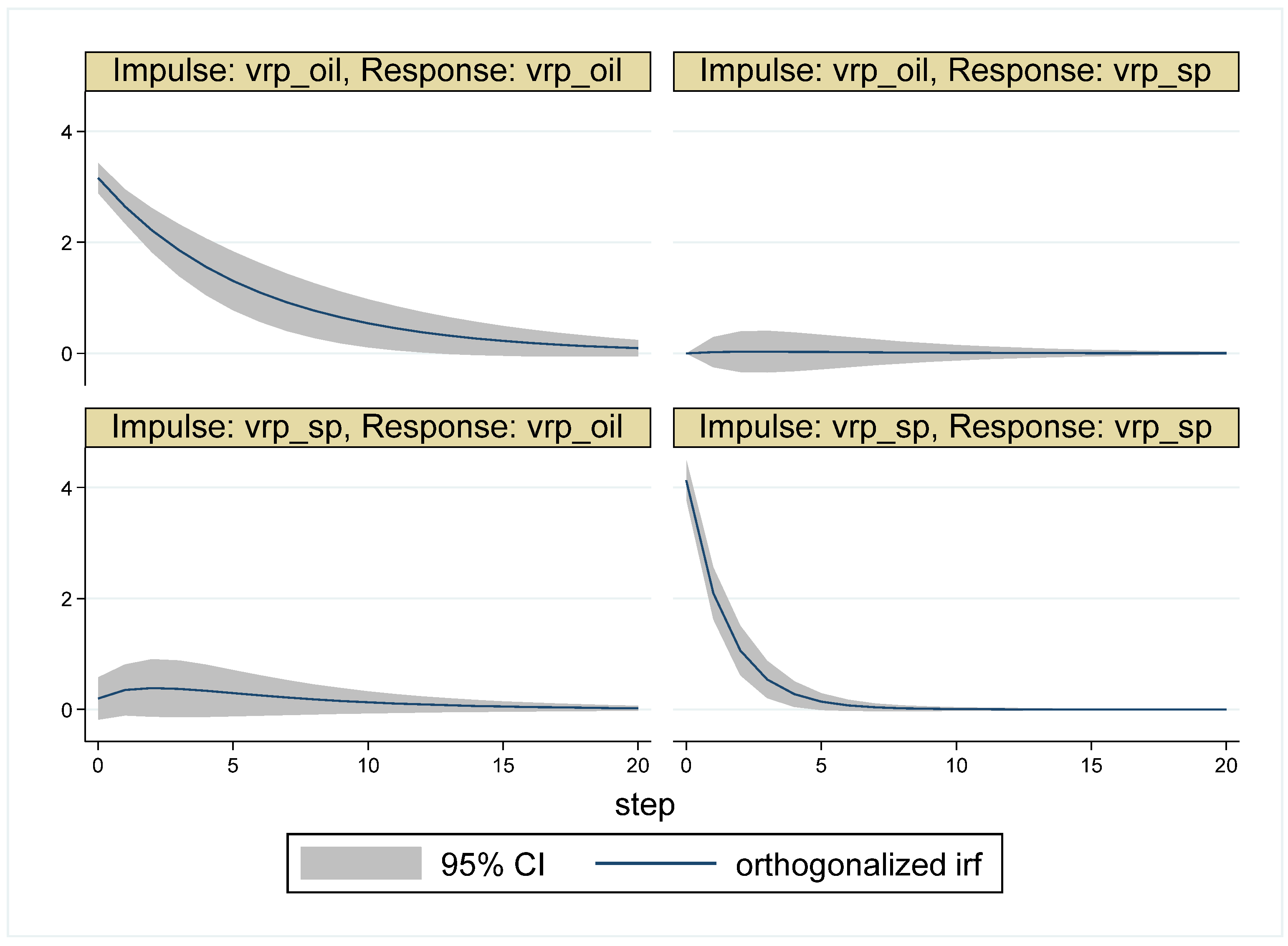
Figure 3 shows the orthogonalized impulse response functions of stock and oil VRP with 95% confidence intervals where we order VRP oil before VRP sp .10 The impulse response functions of VRP sp to VRP oil shown in the above-right graph are significantly positive until date 14, as the lower bounds of their 95% confidence intervals are larger than zero, and gradually decrease toward date 20. Likewise, the impulse response functions of VRP oil to VRP sp shown in the below-left graph are significantly positive until date 17, except for dates 3 and 4, and tend to decrease toward date 20. Thus, if we look at the whole period, shocks in both VRP sp and VRP oil have, though small, significantly positive effects on each other for most of the 20 trading days (about 1 month) after the shock.
The variance decomposition results are listed in Table 6. Shocks to VRP sp explained by innovations in VRP oil are shown in the fourth column, which indicates that 5.2% of the forecast-error variance of VRP sp is explained by innovations in VRP oil on date 20. Meanwhile, shocks to VRP oil explained by innovations in VRP sp are shown in the third column, which indicates that 2.7% of the forecast-error variance of VRP oil is explained by innovations in VRP sp on date 20.
Thus, for the whole period, the VRP of stock and oil have similar (i.e., small but significantly positive) effects on each other. That is, investors’ sentiments in the stock and oil markets affect each other similarly in the sense that an increase in the premium for volatility risk in one market propagates to the other market, although the effect is not large.

5.2. Results for the Sub-Periods

If we see the relations between the VRP of stock and oil in the sub-periods, however, we have rather different pictures. Table 7 shows the results of the Granger causality tests for the sub-periods.
It is interesting that the stock VRP Granger causes the oil VRP very strongly at the 1% significance level in the post-crisis recovery period I (i.e., Period 3), but not in the other sub-periods except for the plunging oil price period (i.e., Period 5) in which VRP sp Granger causes VRP oil only at 10% significance level. In contrast, the oil VRP Granger causes the stock VRP strongly at the 1% significance level in the post-crisis recovery periods (i.e., periods 3 and 4) and relatively strongly at the 5% significance level in the crisis outbreak and the plunging oil price periods (i.e., Periods 2 and 5, respectively). Thus, while the Granger causality from VRP sp to VRP oil over the entire period is mainly from that in post-crisis recovery period I (i.e., Period 3), the Granger causality from VRP oil to VRP sp is persistent after the outbreak of the crisis.
The results of the Granger causality test suggest that the Granger causality is stronger and more persistent from oil to stock than from stock to oil. We show only the results for which VRP oil is ordered before VRP sp in the following analyses of orthogonalized impulse response functions and variance decomposition.
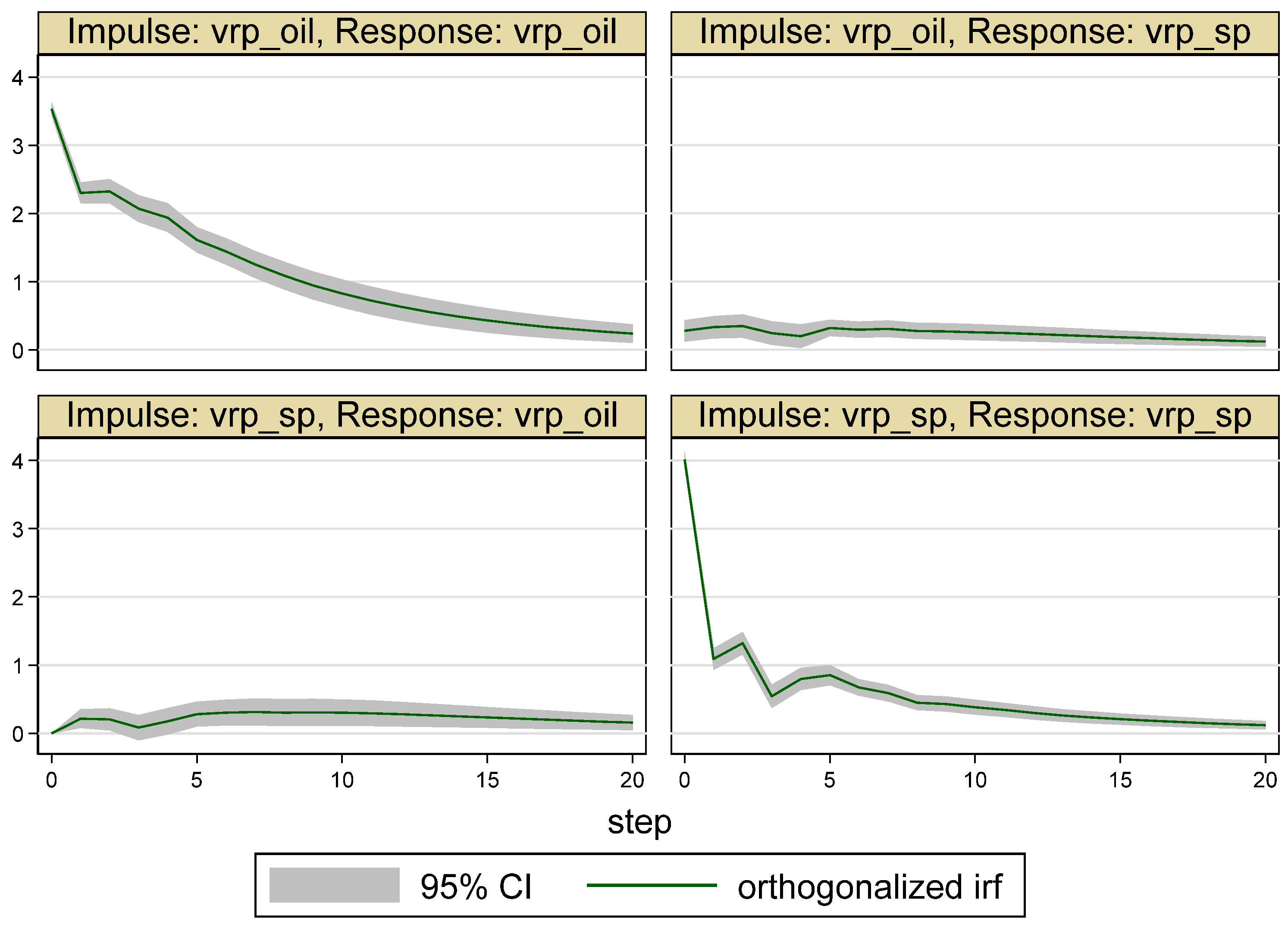
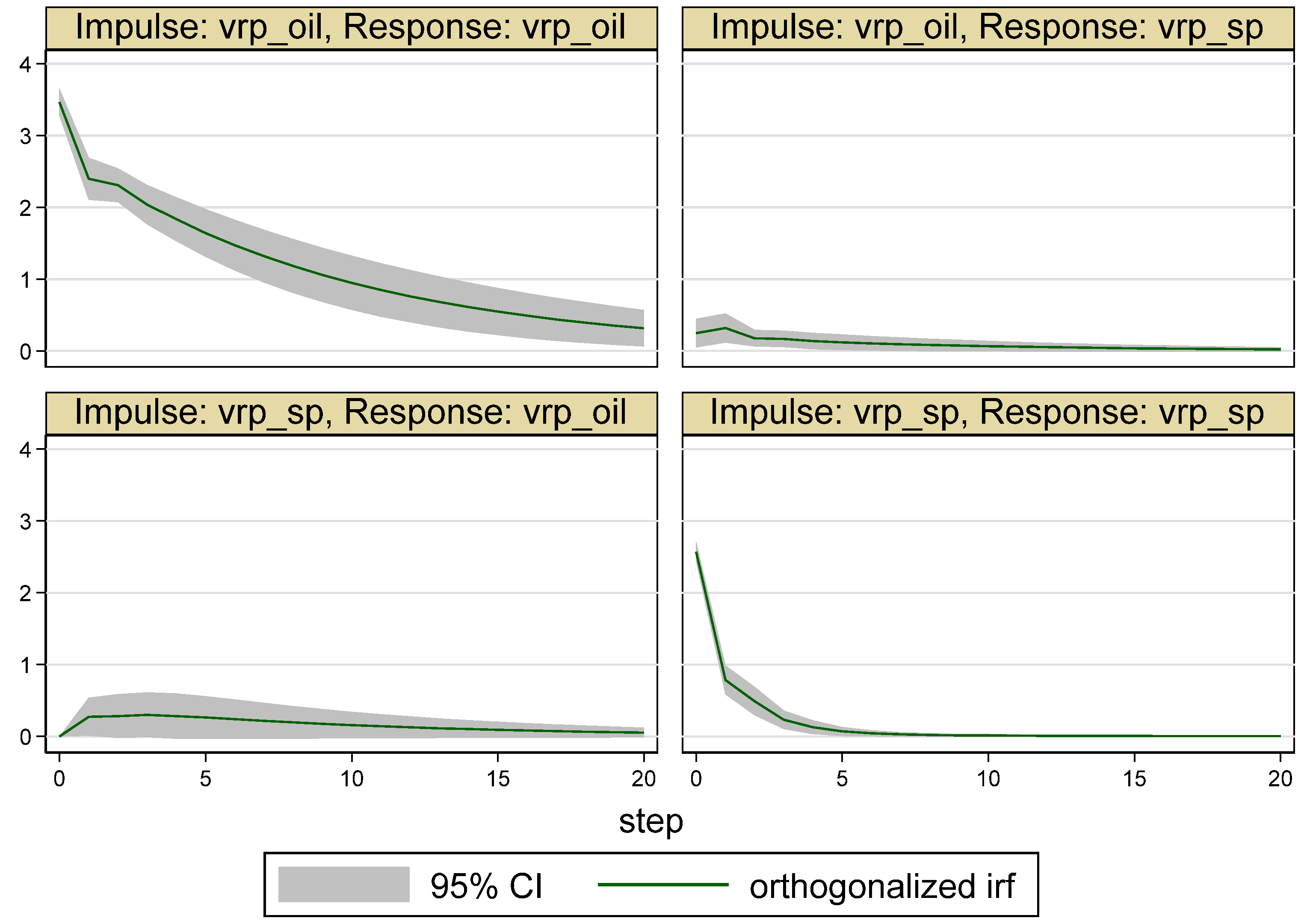
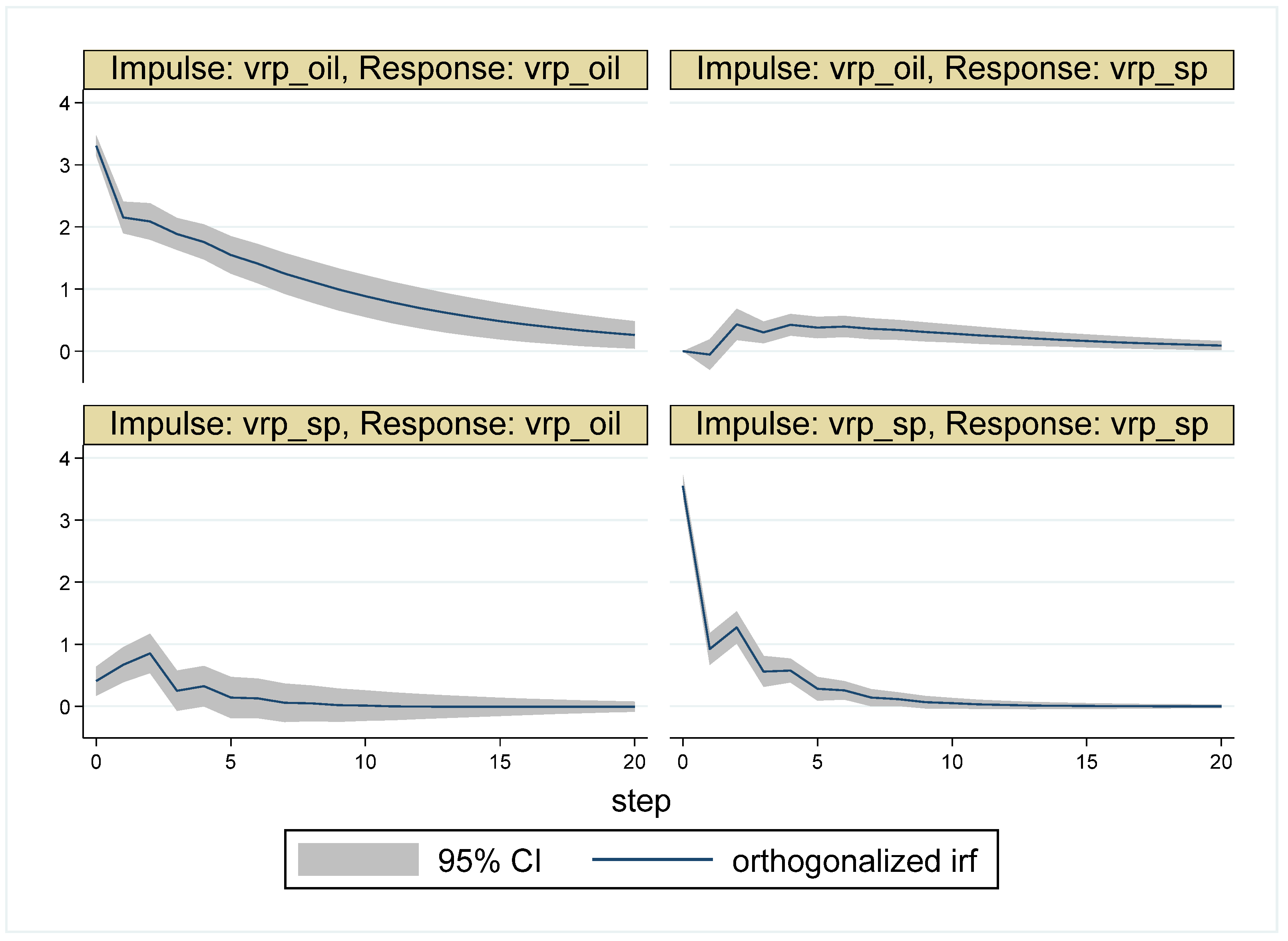
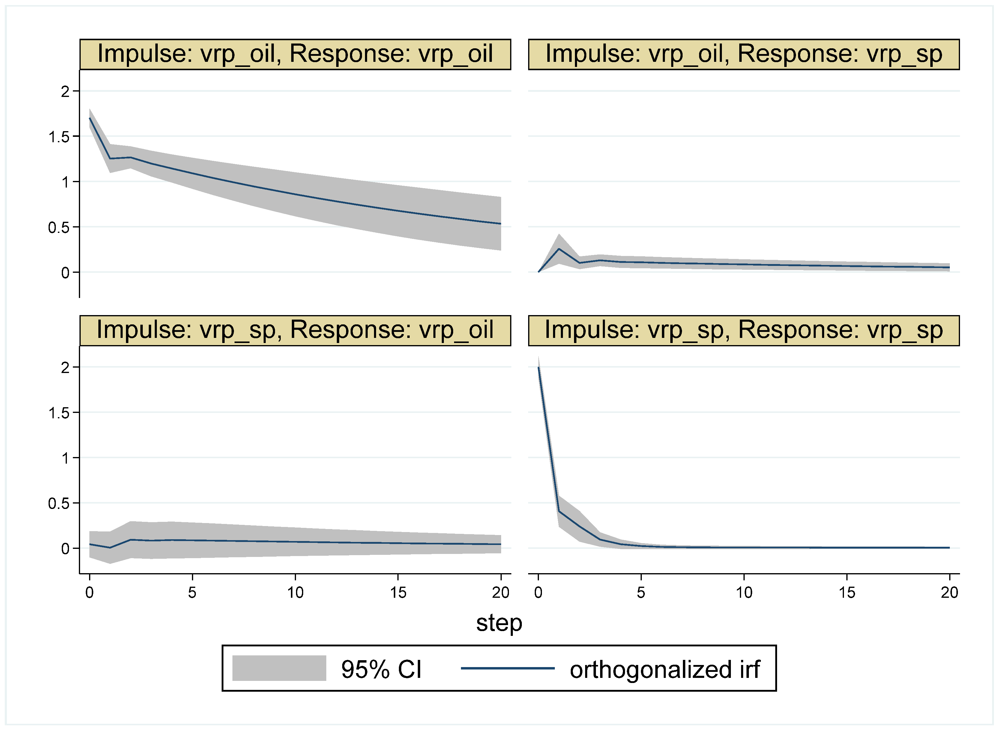
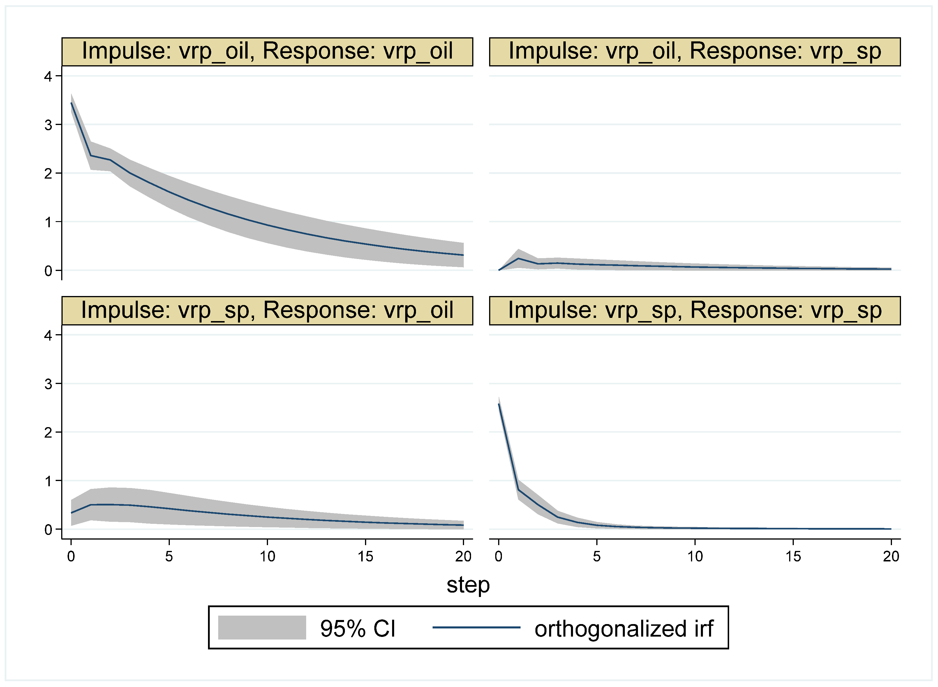
The impulse response functions for each sub-period are shown in Figure 4, Figure 5, Figure 6, Figure 7 and Figure 8. As the graphs at the bottom-left of Figure 4, Figure 5, Figure 6, Figure 7 and Figure 8 show, in the sub-periods the stock VRP has little effect on the oil VRP. Indeed, there are no significant effects from VRP sp to VRP oil except in the post-crisis recovery period I (i.e., Period 3), but even in that period the effects are short-lived and significant only up to the 2nd trading day after the shock, as the lower-bounds of the 95% confidence level of the below-left graph in Figure 6 show.
In contrast, as the graphs on the above-right of Figure 5, Figure 6, Figure 7 and Figure 8 show, the oil VRP has, though small, significantly positive and long-lasting effects on stock VRP after the outbreak of the crisis (i.e., in Periods 2, 3, 4, and 5). For example, in the crisis outbreak period (i.e., period 2), as the above-right graph of Figure 5 shows, the orthogonalized impulse response functions from VRP oil to VRP sp are significantly positive from the 1st to the 8th trading days after the shock. In post-crisis recovery period I (i.e., Period 3), as shown in Figure 6, they are significantly positive in all but the 1st trading day. In post-crisis recovery period II (Period 4), as shown in Figure 7, they are significantly positive in all trading days after the shock. Finally, in the plunging oil price period (i.e., Period 5), as shown in Figure 8, they are significantly positive up to the 7th trading day. Consistent with the Granger causality tests, those results of the impulse response functions in the sub-periods suggest that the oil VRP dynamically affects the stock VRP, but not vice versa.
Table 8 shows the results of the variance decomposition for the sub-periods. The shocks to VRP oil explained by innovations in VRP sp are shown in the third column, and the shocks to VRP sp explained by innovations in VRP oil are shown in the fourth column. Similar to the results of the Granger causality tests and impulse response functions, the forecast error variances of the oil VRP explained by innovations in the stock VRP are much smaller than those of the stock VRP explained by the oil VRP in all sub-periods except the pre-crisis period (Period 1). For example, on date 20, the forecast-error variances of VRP oil ( VRP sp ) explained by innovations in VRP sp ( VRP oil ) are 0.011 (0.005), 0.009 (0.080), 0.015 (0.114), 0.002 (0.048), and 0.015 (0.040) in periods 1, 2, 3, 4, and 5, respectively. Again, the oil VRP dynamically affects the stock VRP much more than the stock VRP does, which dynamically affects the oil VRP after the financial crisis.
Thus, the analyses of the sub-periods reveal that the dynamic relationship between the stock and oil VRP depends on the economic situation and, more importantly, that the VRP of oil has long-lasting and significantly positive effects on that of stock after the outbreak of the financial crisis, whereas the effects of the stock VRP on the oil VRP are limited and, if any, much more short-lived. That is, investors’ sentiments propagate from the oil market to the stock market after the global financial crisis, but not from the stock market to the oil market, except in the first half of the recovery period after the financial crisis.

6. Robustness Analysis

To check the robustness of the results in orthogonalized impulse response functions and variance decomposition, we repeat the analysis by reversing the order of the VRP to place VRP sp before VRP oil . The results are quite similar to those above, although the effects of VRP sp on VRP oil (resp. VRP oil on VRP sp ) become slightly stronger (resp. weaker) than those previously obtained.
For example, Figure 9, Figure 10, Figure 11, Figure 12 and Figure 13 show the orthogonalized impulse response functions for the sub-periods. The figures are qualitatively the same as those above.
Table 9 shows the results of the variance decomposition focusing on the 20th trading day after the shocks. This table shows that the forecast-error variances of oil (resp. stock) VRP explained by the innovation in the stock (resp. oil) VRP are now generally larger (resp. smaller) than those in the previous case. For example, in Period 3, the forecast error variance of VRP oil (resp. VRP sp ) explained by VRP sp (resp. VRP oil ) is 0.039 (resp. 0.084) on the 20th day after the shock, whereas the corresponding values in the case above are 0.015 (resp. 0.114).
Similarly, we repeat the analysis using different lag lengths, although not optimal, to see how the results can change. We choose lag lengths equal to 4 and 9 because the former corresponds roughly to 1 week (5 trading days) coverage and the latter to 2 weeks (10 trading days). We do not report the results here, but they are qualitatively the same as those obtained above while the effects of stock on oil seem to be slightly stronger.

7. Summary and Concluding Remarks

The VRP was found to have predictive power for returns in many different assets. While most extant studies have analyzed the predictability of VRP on asset returns, this study investigated how the VRP of different assets, specifically those of stock and oil, are dynamically related to each other. To this end, we obtained stock VRP as the difference between the VIX published by the CBOE and the realized volatility of the S&P 500 stock index provided by the Oxford–Man Institute of Quantitative Finance. In contrast, to construct the oil VRP, we estimated the realized volatility of the USO by a stochastic volatility model and subtracted it from the OVX published by the CBOE.
Using daily data from 10 May 2007 to 16 May 2017, we conducted VAR analyses on the stock and oil VRP for the whole period and five sub-periods that represent the pre-crisis, crisis outbreak, post-crisis recovery (the first and the second half) and plunging oil price periods.
The analysis of the whole period shows that the VRP of stock and oil have similar (i.e., small but significantly positive) effects on each other. However, the analyses of the five sub-periods revealed a different picture. The dynamic relationship between the stock and oil VRP depends on the economic situation and, contrary to the results for the whole period, the effects of the stock and oil VRP on their counterparts are quite different: The effects of the stock VRP on the oil VRP are limited mainly in the first half of the post-crisis recovery period and are short-lived. in contrast, the VRP of oil has significantly positive and long-lasting effects on that of stock in all sub-periods after the outbreak of the financial crisis.
It is worth pointing out that those results suggest that the investors’ sentiments (measured by volatility risk premia) are transmitted from the oil market to the stock market over time, but not the other way around. While Christoffersen and Pan (2018) find the predictability of oil implied volatility on stock returns and implied volatility, the relationship between oil and stock VRP is still an unexplored point in the extant literature and is a rather unexpected finding because the financialization of commodities means a massive increase in investment in commodities by the investors in the traditional stock and bond markets; hence, the direction of the effects is thought to be from the stock market to the commodity market, and not from the commodity market to the stock market.
However, the mechanism of such a transmission of VRP from oil to stock has not yet been elucidated. One possible channel is the funding constraints of financial intermediaries. Christoffersen and Pan (2018) found that increases in oil implied volatility predict tightening funding constraints of financial intermediaries, which can affect stock price and implied volatility; the oil VRP may affect the stock VRP through institutional investors’ funding constraints. Hattori et al. (2021) found that increases in the U.S. stock VRP tend to reduce the fund flow into stocks of emerging economy countries and suggested that this can be the cause of the spillover of VRP among countries. One may also speculate that the tendency of declining oil prices after the financial crisis and the emergence of shale oil/gas may make investments in U.S. stocks by petroleum-exporting countries (i.e., “petrodollars”) more sensitive to the future uncertainty of oil prices, to which other investors become more sensitive. Investigating what causes oil VRP to affect stock VRP is an important target for future research.
In addition, owing to the constraint on data availability, we must estimate the realized volatility by applying a stochastic volatility model to the daily data of the USO returns. This makes our estimation of the oil VRP, which is the difference between the OVX published by the CBOE and the realized volatility calculated, prone to the misspecification of the used model. To utilize the same estimation method as the stock VRP, or more specifically as the stock-realized volatility, it is desirable to estimate the realized volatility of the USO using intraday 5 min return data. Such a method also enables us to investigate the relationship among the returns and VRP of stock and oil. This is another important topic for future research.
Finally, analyzing the relationship among the returns and VRP of stock and oil helps investors and policy makers understand how the returns and sentiment of one market affect those of the other market. Indeed, the results of this study show that, after the global financial crisis, the shock in investor sentiment on oil prices propagates to that on stock prices, but not vice versa. This means that it is important for investors and policy makers to pay more attention to the spillover of shocks from oil to stock than from stock to oil in order to attain better risk management and asset allocation. Therefore, the direction of this study is fruitful.

Author Contributions

Conceptualization, N.N. and K.O.; Methodology, N.N., K.O. and D.Y.; Formal analysis, N.N., K.O. and D.Y.; Data curation, D.Y.; Writing—original draft, K.O.; Writing—review & editing, K.O.; Project administration, K.O.; Funding acquisition, N.N. and K.O. All authors have read and agreed to the published version of the manuscript.

Funding

This research was funded by Japan Society for the Promotion of Science grant number 21H00727.

Data Availability Statement

We calculate the daily stock VRP as the difference between the VIX index and the daily realized volatility of the S&P 500 stock index. The data of VIX index can be obtained from the CBOE home page https://www.cboe.com/us/indices/dashboard/VIX/ (accessed on 26 December 2022). The data of daily realized volatility of the S&P 500 stock index is provided by the Oxford-Man Institute of Quantitative Finance http://realized.oxford-man.ox.ac.uk/ (accessed on 26 December 2022). The daily oil VRP is calculated as the difference between the OVX and the daily realized volatility of USO, which is the underlying asset of OVX. The data of OVX is available from the CBOE home page https://www.cboe.com/us/indices/dashboard/OVX/ (accessed on 26 December 2022). The daily realized volatility is estimated by the stochastic volatility model (explained in Appendix A) using the data of daily USO returns, which is purchased from Refinitiv.

Acknowledgments

This study was conducted in the project “Economic and Financial Analysis of Commodity Markets” at the Research Institute of Economy, Trade and Industry (RIETI). We are grateful to Katja Ignatieva, Kentaro Iwatsubo, Katsushi Nakajima, Hiroshi Ohashi, Tatsuyoshi Okimoto, Makoto Takahashi, Tianyang Wang, Yuji Yamada, Makoto Yano, and all seminar participants at the AJRC and RIETI workshops on economic and financial analysis of commodity markets in ANU, the Discussion Paper seminar at RIETI (RIETI DP 18-E-027), the fourth annual J.P. Morgan Center for Commodities International Symposium, and anonymous referees for their helpful comments and discussions. Nakamura and Ohashi acknowledge financial support from Grants-in-Aid for Scientific Research (21H00727) by Japan Society for the Promotion of Science.

Conflicts of Interest

The authors declare no conflict of interest.

Appendix A. Estimation of Realized Volatility by a Stochastic Volatility Model

We estimate the daily realized volatility of oil by applying the following stochastic volatility model to its return.
r oil   t = μ oil + β oil ( e h t 2 OVX t ) + e h t 2 ϵ t , h t = μ h + β h ( h t 1 μ h ) + σ h η t , ϵ t ν 2 ν ξ t ζ t ,   ζ t Γ ( ν / 2 , ν / 2 ) , ( ξ t η t ) ~ N ( ( 0 0 ) , [ 1 ρ ρ 1 ] )
where r oil   t denotes the daily return of the USO, N ( ) denotes the bivariate standard normal distribution with correlation ρ , and Γ ( ν / 2 , ν / 2 ) denotes the gamma-distribution with shape and scale parameters equal to ν / 2 . Here, realized volatility is estimated as RV oil   t = e h t 2 .
We estimated the model for the five sub-periods using Bayesian statistical inference according to the widely applicable information criterion (WAIC). The estimates of mean, 5%, and 95% percentile points (in parentheses) are as follows:
Table A1. Estimates of mean and standard deviation of parameters.
ParameterPeriod 1Period 2Period 3Period 4Period 5
μ oil 0.305
(0.192, 0.415)
−0.336
(−0.496, −0.178)
−0.017
(−0.03, −0.01)
0.007
(0.003, 0.010)
−0.194
(−0270, −0.122)
β oil 0.041
(−0.039, 0.123)
0.068
(−0.017, 0.151)
0.032
(−0.044, 0.109)
0.028
(−0.046, 0.101)
0.085
(0.004, 0.164)
μ h 1.232
(0.936, 1.530)
2.472
(2.084, 2.820)
1.278
(1.134, 1.428)
0.292
(0.095, 0.509)
1.675
(1.413, 1.939)
β h 0.849
(0.774, 0.915)
0.891
(0.835, 0.940)
0.809
(0.733, 0.873)
0.846
(0.771, 0.903)
0.914
(0.876, 0.946)
σ h 0.380
(0.336, 0.431)
0.369
(0.325, 0.417)
0.363
(0.325, 0.406)
0.368
(0.328, 0.413)
0.349
(0.311, 0.391)
ρ −0.488
(−0.630, −0.335)
−0.4649
(−0.608, −0.310)
−0.467
(−0.587, −0.331)
−0.457
(−0.595, −0.308)
−0.413
(−0.550, −0.269)
ν 8.047
(6.455, 9.753)
8.083
(6.520, 9.757)
8.455
(6.972, 10.116)
8.014
(6.476, 9.664)
8.534
(6.994, 10.210)

Notes

1
Results by extant researches about the effects of oil volatility-related variables on stock returns and volatility are mixed. For example, Ornelas and Mauad (2019) find little predictability of oil VRP on S&P 500 returns, Bams et al. (2017) find that difference of oil VRP is priced only on returns of oil-related stocks, and Christoffersen and Pan (2018) find predictability of oil implied volatility on stock returns and implied volatility.
2
Volatility swap and variance swap, where variance is the square of volatility, are traded in over-the-counter derivative markets.
3
Ornelas and Mauad (2019) explain what kind of realized volatility is used in the literature to approximate the expected future volatility.
4
5
6
7
Appendix A explains how we estimate the realized volatility of oil.
8
For Augmented Dickey–Fuller (ADF), Dickey–Fuller–GLS (DF–GLS), and Phillips–Perron (PP) tests, see Dickey and Fuller (1979); Elliott et al. (1996); and Phillips and Perron (1988), respectively.
9
Analyses with different lag length provide results quite similar to those in this paper.
10
We obtain the similar result if we reverse the order of VRP oil and VRP sp . We select this ordering since the results of Granger causality tests show more persistent Granger causality from oil to stock than from stock to oil for most of the sub-periods. For more detail, see next subsection.

References

  1. Bams, Dennis, Gildas Blanchard, Iman Honarvar, and Thorsten Lehnert. 2017. Does oil and gold price uncertainty matter for the stock market? Journal of Empirical Finance 44: 270–85. [Google Scholar] [CrossRef]
  2. Bollerslev, Tim, George Tauchen, and Hao Zhou. 2009a. Expected Stock Returns and Variance Risk Premia. Review of Financial Studies 22: 4463–92. [Google Scholar] [CrossRef]
  3. Bollerslev, Tim, James Marrone, Lai Xu, and Hao Zhou. 2009b. Stock Return Predictability and Variance Risk Premia: Statistical Inference and International Evidence. Journal of Financial and Quantitative Analysis 60: 633–61. [Google Scholar] [CrossRef] [Green Version]
  4. Bouri, Elie, Brian Luceyb, and David Roubaudca. 2020. Dynamic and determinants of spillovers across the option-implied volatilities of US equities. Quarterly Review of Economics and Finance 75: 257–64. [Google Scholar] [CrossRef]
  5. Bouri, Elie, Xiaojie Lei, Yahua Xu, and Hongwei Zhang. 2023. Connectedness in implied higher-order moments of precious metals and energy markets. Energy 263: 125588. [Google Scholar] [CrossRef]
  6. Christoffersen, Peter, and Xuhui (Nick) Pan. 2018. Oil volatility risk and expected stock returns. Journal of Banking and Finance 95: 5–26. [Google Scholar] [CrossRef] [Green Version]
  7. Della Corte, Pasquale, Tarun Ramadorai, and Lucio Sarno. 2016. Volatility risk premia and exchange rate predictability. Journal of Financial Economics 120: 21–40. [Google Scholar] [CrossRef]
  8. Dickey, David A., and Wayne A. Fuller. 1979. Distribution of the Estimators for Autoregressive Time Series with a Unit Root. Journal of the American Statistical Association 74: 427–31. [Google Scholar] [CrossRef]
  9. Diebold, Francis X., and Kamil Yilmaz. 2014. On the network topology of variance decomppositions: Measuring the connectedness of financial firms. Journal of Econometricss 182: 119–34. [Google Scholar] [CrossRef] [Green Version]
  10. Dutta, Anupam, Elie Bourib, and David Roubaud. 2019. Nonlinear relationships amongst the implied volatilities of crude oil and precious metals. Resources Policy 61: 473–78. [Google Scholar] [CrossRef]
  11. Elliott, Graham, James H. Stock, and Thomas J. Rotenberg. 1996. Efficient Tests for an Autoregressive Unit Root. Econometrica 64: 813–36. [Google Scholar] [CrossRef] [Green Version]
  12. Gagnon, Marie-Helene, Gabriel J. Power, and Dominique Toupin. 2015. Dynamics between crude oil and equity markets under the risk-neutral measure. Applied Economics Letters 22: 370–77. [Google Scholar] [CrossRef]
  13. Hattori, Masazumi, Ilhoyock Shim, and Yoshihiko Sugihara. 2021. Cross-stock market spillovers through variance risk premiums and equity flows. Journal of International Money and Finance 119: 102480. [Google Scholar] [CrossRef]
  14. Iqbal, Najaf, Elie Bouri, Guangrui Liu, and Ashish Kumar. 2022. Volatility spillovers during normal and high volatility states and their driving factors: A cross-country and cross-asset analysis. International Journal of Finance and Economics, 1–21. [Google Scholar] [CrossRef]
  15. Liu, Ming-Lei, Qiang Ji, and Ying Fan. 2013. How does all market uncertainty interact with other markets? An empirical analysis of implied volatility index. Energy 55: 860–68. [Google Scholar] [CrossRef]
  16. Londono, Juan, and Hao Zhou. 2016. Variance Risk Premiums and the Forward Premium Puzzle. Journal of Financial Economics 124: 415–40. [Google Scholar] [CrossRef] [Green Version]
  17. Ohashi, Kazuhiko, and Tatsuyoshi Okimoto. 2016. Increasing Trends in the Excess Comovement of Commodity Prices. Journal of Commodity Markets 1: 48–64. [Google Scholar] [CrossRef] [Green Version]
  18. Ornelas, Jose Renato Haas, and Roberto Baltieri Mauad. 2019. Volatility risk premia and futures commodities returns. Journal of International Money and Finance 96: 341–60. [Google Scholar] [CrossRef]
  19. Phillips, Peter C. B., and Pierre Perron. 1988. Testing for a Unit Root in Time Series Regression. Biometrika 75: 335–46. [Google Scholar] [CrossRef]
  20. Robe, Michel A., and Jonathan Wallen. 2016. Fundamentals, Derivatives Market Information and Oil Price Volatility. Journal of Futures Markets 36: 317–44. [Google Scholar] [CrossRef]
  21. Silvennoinen, Annastiina, and Susan Thorp. 2013. Financialization, Crisis and Commodity Correlation Dynamics. Journal of International Financial Markets Institutions & Money 24: 42–65. [Google Scholar] [CrossRef] [Green Version]
  22. Tang, Ke, and Wei Xiong. 2012. Index Investment and the Financialization of Commodities. Financial Analysts Journal 68: 54–74. [Google Scholar] [CrossRef]
  23. Zhang, Xinxin, Elie Bouri, Yahua Xu, and Gongqiu Zhang. 2022. The asymmetric relationship between returns and option-implied higher moments: Evidence from the crude oil market. Energy Economics 109: 105950. [Google Scholar] [CrossRef]
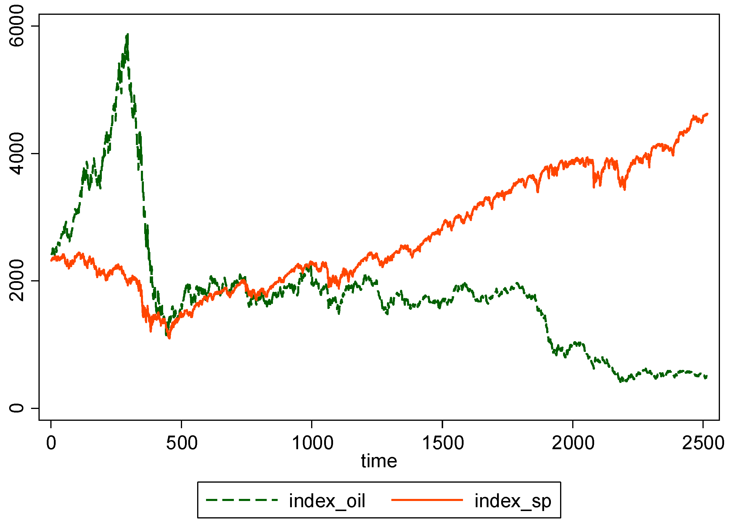
Figure 1. index_sp (S&P 500) and index_oil (USO multiplied by 50). Notes: Daily oil index (USO) multiplied by 50 and stock index (S&P 500) from 10 May 2007 to 16 May 2017 where the vertical axis is measured in U.S. dollars and time in the horizontal axis represents the date where time 1 corresponds to 10 May 2007, time 500 to 13 May 2009, time 1000 to 6 May 2011, time 1500 to 3 May 2013, time 2000 to 29 April 2015, and time 2500 to 24 April 2017, respectively.
Jrfm 16 00173 g001
Figure 2. VRP oil and VRP sp from 10 May 2007 to 16 May 2017. Notes: Daily volatility risk premium of oil ( VRP oil ) and stock ( VRP sp ) from 10 May 2007 to 16 May 2017. The vertical axis represents their values and time in the horizontal axis represents the date where time 1 corresponds to 10 May 2007, time 500 to 13 May 2009, time 1000 to 6 May 2011, time 1500 to 3 May 2013, time 2000 to 29 April 2015, and time 2500 to 24 April 2017, respectively.
Jrfm 16 00173 g002
Figure 3. Impulse response functions (whole period). Notes: Vrp_oil (resp. vrp_sp) represents volatility risk premium of oil (resp. stock). The solid line represents orthogonalized impulse response functions and the gray area represents their 95% confidence intervals. The above-right graph shows the impulse response functions of vrp_sp to vrp_oil. The below-left graph shows the impulse response functions of vrp_oil to vrp_sp.
Jrfm 16 00173 g003
Figure 4. Impulse Response Function (Period 1).
Jrfm 16 00173 g004
Figure 5. Impulse Response Function (Period 2).
Jrfm 16 00173 g005
Figure 6. Impulse Response Function (Period 3).
Jrfm 16 00173 g006
Figure 7. Impulse Response Function (Period 4).
Jrfm 16 00173 g007
Figure 8. Impulse Response Function (Period 5). Notes: Vrp_oil (resp. vrp_sp) represents volatility risk premium of oil (resp. stock). The solid line represents orthogonalized impulse response functions and the gray area represents their 95% confidence intervals. The above-right graph shows the impulse response functions of vrp_sp to vrp_oil. The below-left graph shows the impulse response functions of vrp_oil to vrp_sp.
Jrfm 16 00173 g008
Figure 9. Impulse Response Function with Order VRP sp before VRP oil (Period 1).
Jrfm 16 00173 g009
Figure 10. Impulse Response Function with Order VRP sp before VRP oil (Period 2).
Jrfm 16 00173 g010
Figure 11. Impulse Response Function with Order VRP sp before VRP oil (Period 3).
Jrfm 16 00173 g011
Figure 12. Impulse Response Function with Order VRP sp before VRP oil (Period 4).
Jrfm 16 00173 g012
Figure 13. Impulse Response Function with Order VRP sp before VRP oil (Period 5). Notes: Vrp_oil (resp. vrp_sp) represents volatility risk premium of oil (resp. stock). The solid line represents orthogonalized impulse response functions and the gray area represents their 95% confidence interval. The above-right graph shows the impulse response functions of vrp_sp to vrp_oil. The below-left graph shows the impulse response functions of vrp_oil to vrp_sp.
Jrfm 16 00173 g013
Table 1. Periods and corresponding dates/time.
Whole Period10 May 2007–16 May 2017
(Time = 1–2516)
Period 1 (Pre-crisis period)10 May 2007–31 May 2008
(time = 1–266)
Period 2 (Crisis outbreak period)1 June 2008–30 June 2009
(time = 267–533)
Period 3 (Post-crisis recovery period I)1 July 2009–31 July 2012
(time = 534–1311)
Period 4 (Post-crisis recovery period II)1 August 2012–30 September 2014
(time = 1312–1855)
Period 5 (Plunging oil price period)1 October 2014–16 May 2017
(time = 1856–2516)
Table 2. Descriptive statistics of VRP sp and VRP oil .
MeanSt. Dev.Skew.Kurt.Corr.#Obs.
VRP sp (Whole)7.7854.891−3.14149.1160.2732516
VRP sp (Period 1)6.5094.794−1.5027.7240.097266
VRP sp (Period 2)9.58310.148−2.77822.3440.278267
VRP sp (Period 3)9.5364.168−4.29149.5950.344778
VRP sp (Period 4)6.4412.115−0.7225.1560.212544
VRP sp (Period 5)6.6162.801−2.39524.8140.222661
VRP oil (Whole)4.2026.627−0.2305.0470.2732516
VRP oil (Period 1)2.5295.8420.1612.5960.097266
VRP oil (Period 2)3.6239.754−0.0613.5180.278267
VRP oil (Period 3)5.8466.317 0.1354.3150.344778
VRP oil (Period 4)4.2314.6190.4913.1340.212544
VRP oil (Period 5)3.1516.724−0.9295.4070.222661
Notes: The upper (resp. lower) part shows descriptive statistics of volatility risk premium of stock, VRP sp , (resp. oil, VRP oil ) for the whole period and sub-periods 1, 2, 3, 4, and 5.
Table 3. Unit root tests of VRP sp and VRP oil .
ADFDF-GLSPP
VRP sp (Whole)−11.991 ***−9.888 ***−1485.051 ***
VRP sp (Period 1)−4.928 ***−4.815 ***−130.293 ***
VRP sp (Period 2)−3.623 ***−3.938 ***−180.399 ***
VRP sp (Period 3)−8.022 ***−7.041 ***−517.148 ***
VRP sp (Period 4)−7.744 ***−7.827 ***−443.083 ***
VRP sp (Period 5)−8.864 ***−8.651 ***−450.466 ***
VRP oil (Whole)−11.445 ***−11.071 ***−370.718 ***
VRP oil (Period 1)−4.447 ***−4.450 ***−43.848 ***
VRP oil (Period 2)−4.476 ***−4.656 ***−62.622 ***
VRP oil (Period 3)−5.895 *** −5.917 ***−111.345 ***
VRP oil (Period 4)−3.628 ***−3.864 ***−32.445 ***
VRP oil (Period 5)−5.982 ***−5.598 ***−92.555 ***
Notes: *** represents significance at 1% level. All tests reject the null hypothesis at the 1% level significance for all periods.
Table 4. Optimal lag length by AIC, HQIC, and SBIC.
AICHQICSBICSelected Length
Whole Period18525
Period 11111
Period 22222
Period 33333
Period 42222
Period 57222
Notes: The second (resp. third and fourth) column shows the optimal lag length given by AIC (resp. HQIC and SBIC) for each period/sub-period. The fifth column shows the lag length that is used in the analysis of this paper.
Table 5. Granger causality test (whole period).
Null HypothesisPeriodChi 2# of Lags
VRP sp does not GC VRP oil Whole21.174 ***5
VRP oil does not GC VRP sp Whole26.076 ***5
Notes: VRP oil (resp. VRP sp ) represents volatility risk premium of oil (resp. stock). *** indicates significance at 1% level.
Table 6. Variance decompositions (whole period).
Impulse V R P o i l V R P s p V R P o i l V R P s p
Response V R P o i l V R P s p
1100.0050.995
50.9960.0040.0200.980
100.9860.0140.0370.963
150.9770.0230.0480.952
200.9730.0270.0520.948
Note: The first column shows the length of horizon. The third (resp. second) column shows the variance decomposition of VRP oil to VRP sp (resp. itself). Also, the fourth (resp. fifth) column shows the variance decomposition of VRP sp to VRP oil (resp. itself).
Table 7. Granger causality tests for sub-periods.
Null HypothesisPeriodChi 2# of Lags
VRP sp does not GC VRP oil Period 11.2141
Period 21.0112
Period 335.073 ***3
Period 41.4392
Period 54.786 *2
VRP oil does not GC VRP sp Period 10.0241
Period 26.861 **2
Period 327.029 ***3
Period 418.452 ***2
Period 59.066 **2
Notes: VRP oil (resp. VRP sp ) represents volatility risk premium of oil (resp. stock). ***, **, and * indicate significance at 1%, 5%, and 10% levels, respectively.
Table 8. Variance decompositions (sub-periods).
Impulse V R P o i l V R P s p V R P o i l V R P s p
Response V R P o i l V R P s p
Period 1
1100.0040.996
50.9920.0080.0050.995
100.9890.0110.0050.995
150.9890.0110.0050.995
200.9890.0110.0050.995
Period 2
1100.0040.996
50.9950.0050.0440.956
100.9920.0080.0700.930
150.9910.0090.0780.922
200.9910.0090.0800.920
Period 3
1100.0150.985113
50.9810.0190.0560.944
100.9850.0150.0950.905
150.9850.0150.1100.890
200.9850.0150.1140.886
Period 4
1100.0010.999
50.9990.0010.0270.973
100.9980.0020.0370.963
150.9980.0020.0440.956
200.9980.0020.0480.952
Period 5
1100.0090.991
50.9900.0100.0320.968
100.9860.0140.0370.963
150.9850.0150.0390.961
200.9850.0150.0400.960
Note: VRP oil (resp. VRP sp ) represents volatility risk premium of oil (resp. stock). The first column shows the length of horizon. The third (resp. second) column shows the variance decomposition of VRP oil to VRP sp (resp. itself). Also, the fourth (resp. fifth) column shows the variance decomposition of VRP sp to VRP oil (resp. itself).
Table 9. Variance decompositions with order VRP sp before VRP oil . (Effects on the 20th trading day after the shock).
Impulse V R P o i l V R P s p V R P o i l V R P s p
Response V R P o i l V R P s p
Period 1
200.9750.02501
Period 2
200.9790.0210.0650.935
Period 3
200.9610.0390.0840.916
Period 4
200.9950.0050.0450.955
Period 5
200.9560.0440.0230.977
Note: VRP oil (resp. VRP sp ) represents volatility risk premium of oil (resp. stock). The first column shows the length of horizon. The third (resp. second) column shows the variance decomposition of VRP oil to VRP sp (resp. itself). Also, the fourth (resp. fifth) column shows the variance decomposition of VRP sp to VRP oil (resp. itself).
Disclaimer/Publisher’s Note: The statements, opinions and data contained in all publications are solely those of the individual author(s) and contributor(s) and not of MDPI and/or the editor(s). MDPI and/or the editor(s) disclaim responsibility for any injury to people or property resulting from any ideas, methods, instructions or products referred to in the content.