Time-Varying Relation between Oil Shocks and European Stock Market Returns

Abstract

This paper considers a time-varying parameter vector autoregression model to analyze the varying impact of three types of structural oil shocks (the supply-side shock, the aggregate demand shock, and the oil-specific demand shock) on the European stock market since the 1990s. Our findings show that the three types of oil shocks heterogeneously influence stock market returns in the euro area, and that this influence considerably changes over time during the period considered. First, an unexpected increase in oil supply appears to exert a positive but generally declining effect in the period before the Global Financial Crisis (GFC) of 2007–2009, which descends into negative values after the GFC. Second, an unanticipated increase in aggregate demand triggers a generally positive effect on stock market returns in the euro area. However, in the period from 2003 to 2005, stock market returns responded negatively, which could be attributed to the so-called growth-retarding effect. Third, an unexpected increase in oil-specific demand instigates a negative response in the pre-GFC period (considering the response 4–5 months after the shock), although this changes to a positive effect thereafter. Interestingly, irrespective of the origin of oil price fluctuations, oil price increases are associated with positive European stock market returns after the GFC. This signals a greater degree of oil market financialization.

1. Introduction

Since the dawn of the modern oil industry era in the 19th century, crude oil has become a catalyst of rapid industrialization and economic growth, and a source of employment, income, and consumption. The crude oil market has been closely monitored by analysts, companies, investors, policy makers, regulators, and researchers. Crude oil has become a strategic imperative for oil-importing countries. It is, therefore, not surprising that news about the crude oil market and prices regularly hit the headlines in the media. Crude oil is both an investable asset included in investment portfolios as a diversification strategy by investors (see Soytas et al. 2009)1 and a key production input.

The relation between crude oil and aggregate stock prices is driven by at least three theoretical channels. First, since crude oil is regarded as an investable asset, investment decisions in the crude oil market may generate firm valuation effects in the stock market, as investors rebalance their portfolios (see Ciner 2013; Ciner et al. 2013). Second, as a key production input, an increase in oil price translates into higher or more uncertain future production costs, which induces firms to reduce or delay both investment and production. Lower investment and production, in turn, cause a reduction in stock prices and returns. Similarly, in periods of heightened uncertainty about shortfalls of expected supply relative to expected demand for crude oil, when future production costs of a firm also become uncertain, an ensuing increase in precautionary (oil-specific) demand is associated with a higher perceived risk of investment and, hence, lower return on the firm’s stock. Third, standard financial theory indicates that expected stock return is determined by changes in expected cash flows and discount rates, which may be influenced by oil prices.2 Admittedly, oil price can affect expected rates of inflation and real interest, the main elements of expected discount rate. For instance, an oil price rise triggers inflationary pressures in oil-importing economies (see, inter alia, Kilian 2008), which leads to an increase in interest rates if central banks pursue inflation targeting (see Bernanke et al. 1997). Such inflationary pressures lead to a higher discount rate, which negatively affects aggregate market returns, and an increase in interest rates makes stock market investments relatively less attractive, which depresses stock prices and returns. Furthermore, when the economy experiences a business cycle expansion, expectations of cash flows and dividends increase in response to aggregate demand growth. Although higher global economic activity is associated with increases in oil demand and price, the negative stock market effect of higher oil prices can be counteracted by the positive revenue growth effects of firms. As the global demand shock has played a primary role in increasing the price of oil since the 2000s, the positive effect on real stock returns dominates the negative one and, consequently, one would expect to observe a parallel rise in both oil price and real stock returns. Therefore, it seems clear that oil prices and stock market returns are connected from a theoretical standpoint.

The empirical literature has broadly studied the effects of oil shocks on financial markets. Whereas in a few instances no evidence of any type of link between oil prices and stock returns is found (see, e.g., Huang et al. 1996), most studies show evidence of such a link. For instance, research documents a negative relation between oil prices and stock market returns for net oil-importing economies (see, inter alia, Jones and Kaul 1996; Park and Ratti 2008), a positive link for net oil-exporting countries (see, e.g., Bjørnland 2009; Ramos and Veiga 2013), an asymmetric link (see, inter alia, Sadorsky 1999), or a non-linear relation (see, inter alia, Ciner 2001; Jiménez-Rodríguez 2015; Basher et al. 2018). Additionally, other authors show evidence of instability in the relation (see, e.g., Aloui et al. 2013; Reboredo and Rivera-Castro 2014). However, to the best of our knowledge, it has been only Kang et al. (2015) who have analyzed the time-varying impact of oil shocks on stock market returns by considering the U.S. case, and there is no study that focuses on whether the effects of oil shocks on European stock market returns are time-varying, and if so, how they look like. This paper seeks to bridge this existing gap in the related empirical literature and analyzes, for the first time, how the response of European stock market returns to oil supply and demand shocks may change over time.

The time-varying relation between changes in oil prices and stock market returns is essential for companies, investors, regulators, and policy makers. For instance, CEOs of companies seeking to hedge against oil price changes may need to dynamically re-evaluate their hedging strategies against oil price increases or rises of uncertainty about shortfalls of expected relative supply of crude oil in order to maximize shareholder value. Stock market investors may also need to dynamically re-assess the optimal hedge ratio of stock over commodity investments to maximize the Sharpe ratio of their portfolio holdings. Financial regulators and policy makers may benefit from a time-varying framework when evaluating the scale of financial instabilities provoked by oil price changes.

Over the last decades, different sources of instability in the relation between oil prices and stock returns have come under scrutiny. Among these sources of instability, the Global Financial Crisis of 2007–2009 (GFC) is regarded as one of the most significant. In this period, oil prices experienced a sharp decline, as stock markets crashed around the world, which reversed the observed negative relation in the pre-GFC period (see, inter alia, Mollick and Assefa 2013; Anzuini et al. 2015; Tsai 2015). After the GFC, both the oil market and the stock market continued a downward trend, shown as a positive relation between both markets (see, inter alia, Filis et al. 2011; Reboredo and Rivera-Castro 2014; Sadorsky 2014). A second source of instability is the financialization of the oil market, which is manifested in the growing volume of trading in oil derivatives, driven by institutional investors and financial intermediaries (such as hedge funds, insurance companies, and pension funds) since 2003. It is worth noting that the volume of trading in commodity futures (including oil futures) grew from USD $15 million in 2003 to USD $200 billion in 2008 (Tang and Xiong 2012). This spectacular growth of investment in commodity futures, particularly driven by the speculative motives of institutional investors, is an indication of the financialization of all commodity markets, including the oil market. This financialization, in turn, can alter the structural relation between changes in oil prices and stock market returns by generating a positive comovement. A third source of instability owes to the presence of speculative bubbles in both oil and stock markets. This source was studied by Miller and Ratti (2009), who examine the long-run relation between oil price and international stock markets from 1971 to 2018 using a vector error correction model with structural breaks, which are detected after May 1980, January 1988, and September 1999. The long-run relation was identified from January 1971 to May 1980 and from February 1988 to September 1999, after which date the long-run equilibrium relation seems to disappear. This disequilibrium coincides with the period when stock price and/or oil price bubbles were detected. A fourth source of instability is the change of investor sentiment in financial markets, studied theoretically by Barberis et al. (1998) and empirically by Narayan and Sharma (2011). The theoretical model features two regimes. Specifically, the investor believes that he/she is in the non-stationary regime (the trending regime) whenever a positive earnings surprise is followed by another positive surprise. However, in the case that a negative surprise follows a positive one, the investor believes that he/she is in the stationary earnings regime (the mean-reverting regime). Thus, significant oil price shocks are likely to change the investor’s belief, which in turn is likely to trigger a structural shift in the relation between oil and stock prices.

Despite a plethora of studies on the relation between crude oil and European stock markets (here we only point out some works), no empirical work considers the instabilities emergent in the last decades and analyzes how the impact of oil shocks on European stock market returns may vary over time. Research into the effects of oil price shocks on a European stock market was pioneered by Jones and Kaul (1996). These authors include the U.K. in their analysis, and they show that traditional rational models cannot explain the negative effect of oil price shocks on UK stock returns. Papapetrou (2001) studies how important oil prices are to explain stock price movements in Greece, and she finds that they are very relevant. Park and Ratti (2008) show evidence of a negative effect of oil price shocks on stock market returns for the twelve European oil-importing economies considered and a positive one for the only oil exporter included. Apergis and Miller (2009) consider eight stock markets, including four European economies (namely, France, Germany, Italy and the U.K.), and find that oil price shocks do not have relevant effects on stock market returns. Bjørnland (2009) finds that the Norwegian stock prices positively respond to higher oil prices. Arouri (2011) examines the relation between oil prices and stock markets for twelve European industrial stock indices and shows a strong significant link for most indices. Moreover, he finds that the nature and sensitivity of the response of stock returns to oil shocks differ across sectors. Wang et al. (2013) show that the reaction of the European stock market depends on the origin of the oil shock and is different for oil-importing and oil-exporting economies. Degiannakis et al. (2014) find that the supply-side and oil-specific demand shocks have no impact on European stock market (the Euro STOXX 50 Index) volatility, but the aggregate demand shocks reduce it.

We aim to study how the responses of European stock market returns to oil-supply and -demand shocks change over time by considering a time-varying parameter vector autoregression (TVP-VAR) model. Specifically, following Kilian (2009), we distinguish among three types of structural oil shocks: the supply-side shock, the aggregate demand shock, and the oil-specific demand shock. This study aims to answer three research questions. First, does the response of the European stock market vary across the three structural oil shocks? Second, does the response of the European stock market to the three structural oil shocks vary over time? Third, how does the European stock market respond (positively or negatively) to such structural shocks?

To address these research questions, we present evidence of the variation over time in the stock market response to the three structural oil shocks. Our research findings indicate that the three types of oil shocks influence heterogeneously stock market returns in the euro area. Moreover, the stock market effects display considerable variation over time during the sample period. The supply-side shock (an unexpected increase in oil supply) appears to exert a positive effect in the pre-GFC period, which descends into negative values after the GFC. The aggregate demand shock related to an unanticipated expansion triggers a generally positive effect on stock market returns in the euro area. However, in the period from 2003 to 2005 stock market returns responded negatively, which could be attributed to the so-called growth-retarding effect (Kilian 2009). Third, the oil-specific demand shock referred to an unexpected increase instigates a negative response in the pre-GFC period (considering the response 4–5 months after the shock), albeit a positive effect thereafter. We argue that the negative effect in the post-GFC period is driven by speculative behavior of investors. Interestingly, after the GFC, irrespectively of the sources of oil price fluctuations, oil price rises are followed by positive European stock market returns. This finding signals a greater degree of oil market financialization.

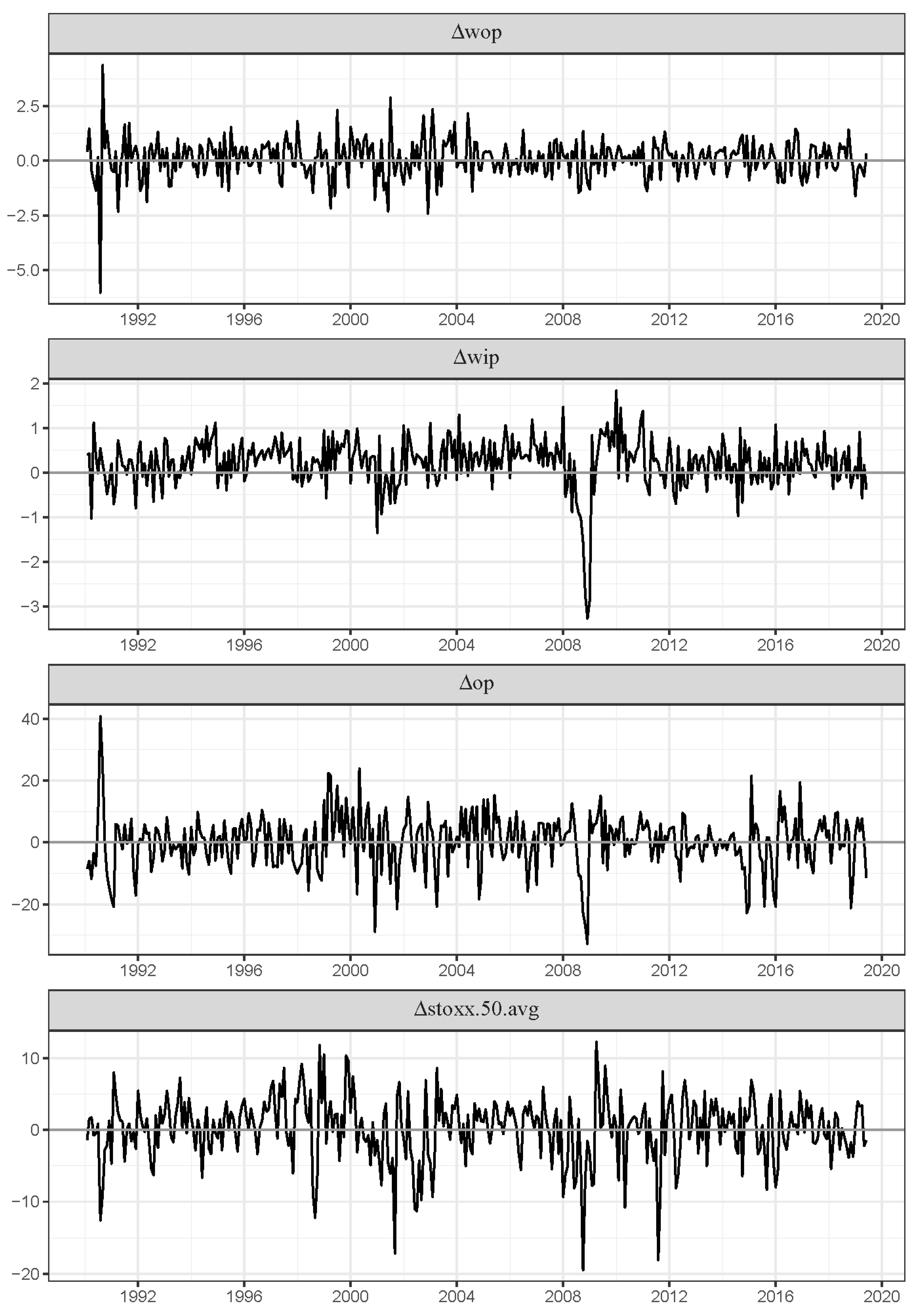
The rest of the paper is organized as follows. Section 2 presents the data and methodology. Section 3 reports the main empirical results. Section 4 concludes.

2. Data and Methodology

Kilian and Park (2009) consider a time-invariant VAR model with two blocks. The first block represents the global crude oil market and includes three variables (a measure of global economic activity, the world crude oil production, and the real oil price), while the second block only contains one variable that represents the U.S. stock market. They use this time-invariant two-block VAR model to study the effects of oil price shocks on the U.S. stock market. Kang et al. (2015) consider the same variables as Kilian and Park (2009) and use a TVP-VAR model to analyze the impact of oil shocks on U.S. stock market returns. Furthermore, Degiannakis et al. (2014) use a time-invariant VAR with a global oil market block and a measure of the volatility of the Euro STOXX 50 index to study the consequences of oil shocks on the volatility of the Euro STOXX 50 index returns. We use a TVP-VAR model that includes the global oil market block (a measure of global economic activity, the world crude oil production, and the real oil price), and a second block that represents the European stock market, measured with the Euro STOXX 50 index.3

2.1. Data

We use the industrial production index of OECD economies + six non-OECD emerging economies (China, India, Indonesia, Brazil, Russia, and South Africa) as a measure of global economic activity, as in Baumeister and Hamilton (2019). It is worth noting that Kilian and Park (2009) consider the economic activity index proposed by Kilian (2009). However, Hamilton (2021) indicates that such an index is misleading and points out that the index that contains the correction made by Kilian (2019) offers a worse indicator of monthly world economic activity than an index of world industrial production.4 Therefore, we follow Hamilton’s (2021) suggestion. The real oil price is calculated by deflating the nominal oil price by the euro area CPI, with the nominal oil price in euros obtained by dividing the nominal Brent crude oil price in dollars by the bilateral euro/dollar exchange rate.5 Data of world crude oil production measured in thousand barrels per day come from the U.S. Energy Information Administration (see https://www.eia.gov/, accessed on 23 November 2019). The real European stock market index is obtained by deflating the Euro STOXX 50 by the euro area CPI. All variables enter the model in first log differences (i.e., $x_t=100\times \left(\log \left(y_t\right)-\log \left(y_{t-1}\right)\right)$ so they can be considered as percentage monthly returns. The common sample runs from 1990:2 to 2019:6.6 We denote the returns on world crude production, industrial production of OECD economies + six non-OECD emerging economies, real oil price and real Euro STOXX 50 by $\Delta wo{p}_t$, $\Delta wi{p}_t$, $\Delta o{p}_t$ and $\Delta stoxx.50.av{g}_t$, respectively.

Figure 1 shows the evolution of the variables included in our TVP-VAR model. All series show considerable variation over time. Episodes of heightened volatility are visible during the GFC, when three of the four return series (returns on world industrial production, oil prices and the Euro STOXX 50 index) experienced significant downswings, particularly in 2008. The return on the Euro STOXX 50 index plummeted again during the European debt crisis in 2010–2012.

Table 1. Descriptive statistics.

Statistics	Δwop	Δwip	Δop	Δstoxx.50.avg
Mean	0.0838	0.2158	0.1631	0.1504
Median	0.1193	0.2851	0.9311	0.8265
Max	4.3763	1.8419	40.8681	12.3041
Min	−6.0423	−3.2652	−32.8454	−19.5042
Sd	0.8990	0.5675	8.8333	4.4824
Skewness	−0.6755	−1.5774	−0.2059	−0.7559
Kurtosis	9.9550	10.5281	5.0237	5.0136
Jarque-Bera (p-value)	738.3198 (0.0000)	979.9280 (0.0000)	62.7303 (0.0000)	93.2482 (0.0000)
ADF (p-value)	−21.0431 (0.0000)	−8.3020 (0.0000)	−14.9236 (0.0000)	−14.0052 (0.0000)

Notes: This table provides descriptive statistics: mean, median, maximum, minimum, standard deviation, skewness, kurtosis and the p-values of both Jarque-Bera and ADF test statistics of the returns on world oil production (Δwop), world industrial production (Δwip), oil prices (Δop) and the Euro STOXX 50 stock index (Δstoxx.50.avg).

presents the descriptive statistics, which are consistent with some stylized facts of financial and economic variables (see Cont 2001). All variables take on average positive values, are leptokurtic, left-skewed and non-normally distributed. The Augmented Dickey-Fuller (ADF) test shows that all returns are stationary.

Table 2. Correlations.

Correlation (p-Value)	Δwop	Δwip	Δop	Δstoxx.50.avg
Δwop	1.0000
Δwip	0.0727	1.0000
	(0.1732)
Δop	−0.0936	0.2545	1.0000
	(0.0791)	(0.0000)
Δstoxx.50.avg	−0.0358	0.1721	0.1136	1.0000
	(0.5024)	(0.0012)	(0.0329)

Notes: This table summarizes the coefficients of correlations among the returns on world oil production (Δwop), world industrial production (Δwip), oil prices (Δop) and the Euro STOXX 50 stock index (Δstoxx.50.avg). p-values are depicted in round parentheses.

summarizes the correlations among the returns. As anticipated, the return on world oil production shows a negative and marginally significant correlation with the return on oil prices (−0.0936). The return on world industrial production comoves positively and significantly with the returns on oil prices (0.2545) and the Euro STOXX 50 stock market index (0.1721). Interestingly, Table 2 also shows a positive correlation between the returns on oil prices and the Euro STOXX 50 stock market index (0.1136), which lends preliminary support to the view that the oil market has become more financialized.

2.2. Methodology

We define $y_t$ as ${\left[\Delta wo{p}_t, \Delta wi{p}_t, \Delta o{p}_t,\Delta stoxx.50.av{g}_t\right]}^{\prime }$. Following Primiceri (2005) and Del Negro and Primiceri (2015), the TVP-VAR model can be written as follows:

$$y_t=a_t+{{\displaystyle \sum }}_{j=1}^p{A}_{j,t}{y}_{t-j}+u_t$$

where $a_t$ is a (4 × 1) vector of time-varying (TV) coefficients that multiply constant terms; $A_{1,t}, \dots ,A_{p,t}$ are (4 × 4) matrices of TV coefficients; and $u_t$ is a (4 × 1) vector of heteroskedastic errors with (4 × 4) variance-covariance matrix ${\mathsf{\Omega }}_{\mathrm{t}}$. The model is rewritten as:

$$y_t=\left(I_4\otimes {x^{\prime }}_t\right){\alpha }_t+u_t$$

where I₄ is a 4-dimensional identity matrix; ⊗ denotes the Kronecker product; ${x^{\prime }}_t=\left[1, {y^{\prime }}_{t-1},\dots ,{y^{\prime }}_{t-p}\right]$is the vector of 1 × (1 + 4p) explanatory variables, and ${\alpha }_t$ is the stacked vector of TV coefficients A_t = (α_t A_1,t … A_p,t). As in Primiceri (2005), we use the triangular reduction of ${\mathsf{\Omega }}_{\mathrm{t}}$:

$$C_t{\mathsf{\Omega }}_{\mathrm{t}}{C}_t^{\prime }={\Sigma }_t{\Sigma }_t^{\prime }$$

where $C_t=\left[\begin{array}{c}1\\ c_{21,t}\\ c_{31,t}\\ c_{41,t}\end{array}\begin{array}{c}0\\ 1\\ c_{32,t}\\ c_{42,t}\end{array}\begin{array}{c}0\\ 0\\ 1\\ c_{43,t}\end{array}\begin{array}{c}0\\ 0\\ 0\\ 1\end{array}\right]$ and ${\Sigma }_t=\left[\begin{array}{c}{\sigma }_{1,t}\\ 0\\ 0\\ 0\end{array}\begin{array}{c}0\\ {\sigma }_{2,t}\\ 0\\ 0\end{array}\begin{array}{c}0\\ 0\\ {\sigma }_{3,t}\\ 0\end{array}\begin{array}{c}0\\ 0\\ 0\\ {\sigma }_{4,t}\end{array}\right]$, with ${\sigma }_{i,t}$ for i = 1, …, 4 being the TV error deviations.

Let $c_t$ be the vector of non-zero and non-one elements of the matrix $C_t$ (stacked by rows), ${c_t=\left(c_{21,t},c_{31,t},c_{32,t},c_{41,t},c_{42,t},c_{43,t}\right)}^{\prime }$. Therefore, the TVP-VAR model can be written as:

$$y_t=\left(I_4\otimes {x^{\prime }}_t\right){\alpha }_t+C_t^{-1}{\Sigma }_t{\epsilon }_t$$

where ${\epsilon }_t$ has I₄ as the variance-covariance matrix. Following Kilian and Park (2009), we use a recursively identified structural model of the form:

$$\left[\begin{array}{c}{u}_t^{\Delta wo{p}_{}}\\ u_t^{\Delta wi{p}_{}}\\ u_t^{\Delta op}\\ u_t^{\Delta stoxx.50.avg}\end{array}\right]=C_t^{-1}{\Sigma }_t\left[\begin{array}{c}{\epsilon }_t^{oil supply shock}\\ {\epsilon }_t^{aggregate demand shock}\\ {\epsilon }_t^{oil specific-demand shock}\\ {\epsilon }_t^{other shocks to stock returns }\end{array}\right]$$

This methodology allows us to identify three oil shocks: (i) oil supply shock, which comes from changes in crude oil production; (ii) aggregate demand shock, which is derived from changes in global economic activity; and (iii) oil-specific demand shock, which comes from innovations to real oil prices unexplained by the other two shocks. The last structural shock ${\epsilon }_t^{other shocks to stock returns }$ refers to innovations to real European stock market returns that are not driven by oil shocks.

The recursive identification scheme implies that European stock market returns may respond instantaneously to the three structural oil shocks and other innovations. This identification scheme rules out instantaneous responses of oil production, global economic activity, or real oil price to the unanticipated stock return. However, lagged responses of these variables are allowed. Underlying the triangular identification scheme is the identifying assumption that the real oil price does not respond contemporaneously to changes in unexpected European stock returns. It implies that the real price of oil is driven by the three oil shocks within the same month. In addition, oil production and global economic activity do not respond contemporaneously to the oil-specific demand shock. Arguably, if global oil supply is running near its capacity limits, expansion of oil production may require investment. However, it takes time for a firm’s investment decision to be reached. In addition, the ensuing investment project is unlikely to materialize within the same month due to physical constraints (Kilian and Lütkepohl 2017, chp. 8.3). Moreover, global economic activity responds to the oil-specific shock with a delay due to a sluggishly changing aggregate demand. Further, global economic activity is ordered second, since higher oil prices driven by disruptions to global oil supply can change consumer and investor confidence within the same month, which induces real spending effects. By contrast, oil supply may not be disrupted by fluctuations in global economic activity within the same month. Such disruptions can occur with a delay, though, as oil producers adjust to the aggregate demand shock. Please see Kilian and Park (2009, scts. 2.2.1 and 2.2.2) and Kilian and Lütkepohl (2017, chp. 8) for further details.

The dynamics of the TV parameters are the following:

$$\begin{gathered} {\alpha }_t={\alpha }_{t-1}+v_t \\ {c}_t=c_{t-1}+{\mathsf{\zeta }}_t \\ \log {\sigma }_t=\log {\sigma }_{t-1}+{\mathsf{\eta }}_t \end{gathered}$$

It is assumed that the error terms (${\epsilon }_t$,$v_t$,${\mathsf{\zeta }}_t$,${\mathsf{\eta }}_t$) are jointly normally distributed with variance covariance matrix V.

$$V=Var\left[\begin{array}{c}{\epsilon }_t\\ v_t\\ {\mathsf{\zeta }}_t\\ {\mathsf{\eta }}_t\end{array}\right]=\left[\begin{array}{c}{I}_4\\ 0\\ 0\\ 0\end{array} \begin{array}{c}0\\ Q\\ 0\\ 0\end{array} \begin{array}{c}0\\ 0\\ S\\ 0\end{array} \begin{array}{c}0\\ 0\\ 0\\ W\end{array} \right]$$

where Q, S and W are positive definite matrices. Moreover, S is block diagonal, with blocks corresponding to parameters belonging to separate equations.

Let ${\alpha }_{}^T$, $C_{}^T$ and ${\Sigma }_{}^T$ be the entire path of parameters ${\left\{{\alpha }_t^{}\right\}}_{t=1}^T$, ${\left\{C_t^{}\right\}}_{t=1}^T$ and ${\left\{{\Sigma }_t^{}\right\}}_{t=1}^T$. To perform Bayesian inference, we use the priors established (following the same principles as in Primiceri 2005) in

Table 3. Prior distributions.

	Parameters
	Prior Family	Coefficients
${\alpha }_0$	$N\left({\widehat{\alpha }}_{OLS},k_{\alpha }\times V\left({\widehat{\alpha }}_{OLS}\right)\right)$	$k_{\alpha }=4$
$C_0$	$N\left({\widehat{C}}_{OLS},k_C\times V\left({\widehat{C}}_{OLS}\right)\right)$	$k_C=$ 4
$\log {\sigma }_0$	$N\left(log{\widehat{\sigma }}_{OLS},k_{\sigma }\times I_4\right)$	$k_{\sigma }=1$
	Hyperparameters
	Prior Family	Coefficients
Q	$IW\left(k_Q^2\times pQ\times V\left({\widehat{\alpha }}_{OLS}\right),pQ\right)$	$k_Q^{}=0.01$ $pQ$ = 60
$S_j, j=1,2,3$	$IW\left(k_s^2\times p{S}_j\times V\left({\widehat{C}}_{j,OLS}\right),p{S}_j\right)$	$k_s^{}=0.1$ $p{S}_j$ = j+1
W	$IW\left(k_W^2\times pW\times I_4,pW\right)$	$k_Q^{}=0.01$ $pW$ = 5

Note: $N$ and $IW$ denote the normal and independent inverse-Wishart distributions, respectively. ${\widehat{\alpha }}_{OLS}, {\widehat{C}}_{OLS}$ and ${\widehat{\sigma }}_{OLS}$are OLS estimates in a time-invariant VAR model for the training sample (which includes 60 observations). $V\left({\widehat{\alpha }}_{OLS}\right)$ and $V\left({\widehat{C}}_{OLS}\right)$ are the estimates of the covariance matrix of ${\widehat{\alpha }}_{OLS}$ and ${\widehat{C}}_{OLS}$, respectively.

.7 This type of inference entails Markov chain Monte Carlo (MCMC)8 posterior simulation methods (Gibbs sampler) for the unobservable states ${\alpha }_{}^T$, $C_{}^T$, ${\Sigma }_{}^T$ and the hyperparameters of the variance-covariance matrix V. The simulations are based on 50,000 iterations for the Gibbs sampler, discarding the initial 5000 burn-in as burn-in sample.9

3. Results

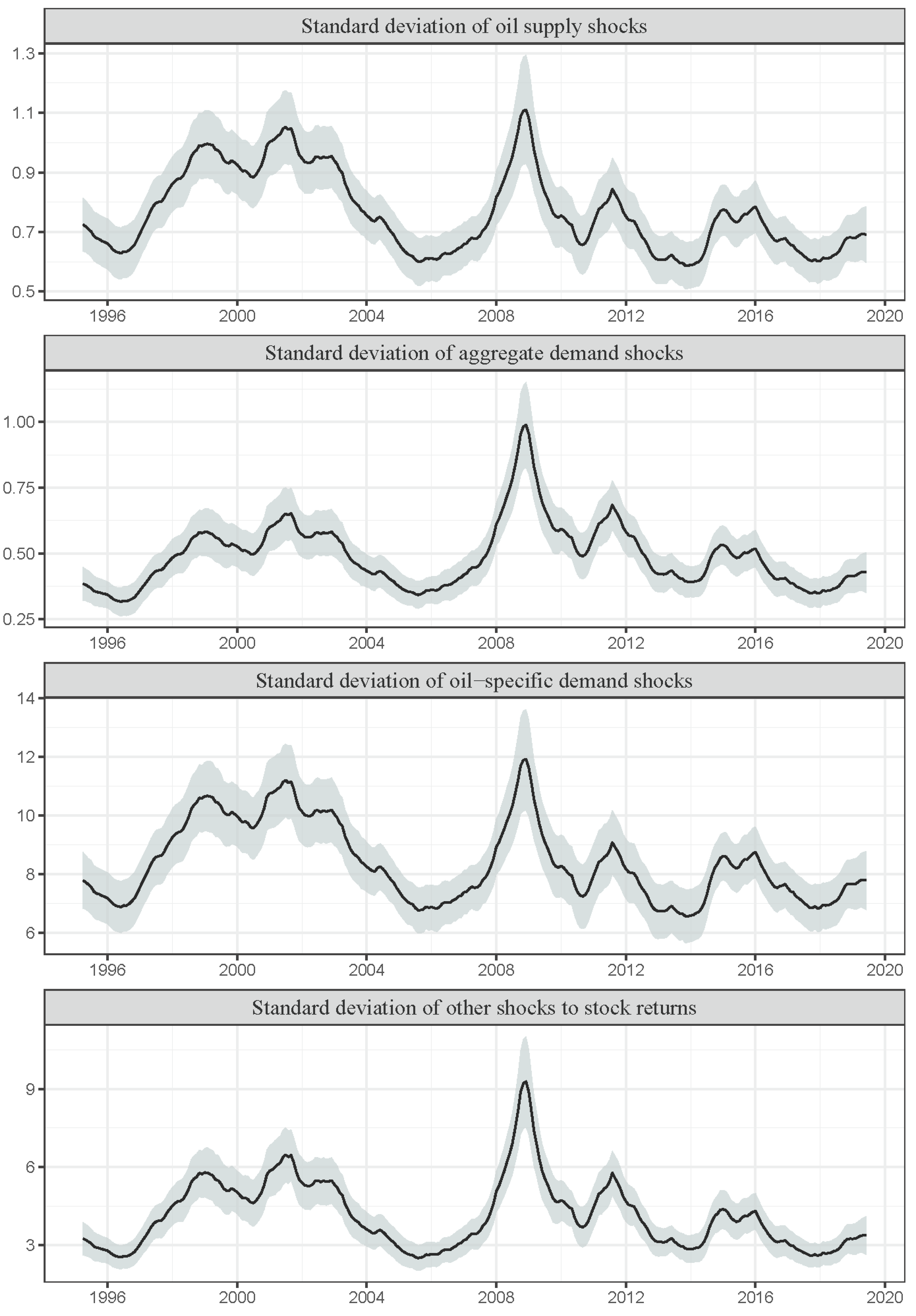
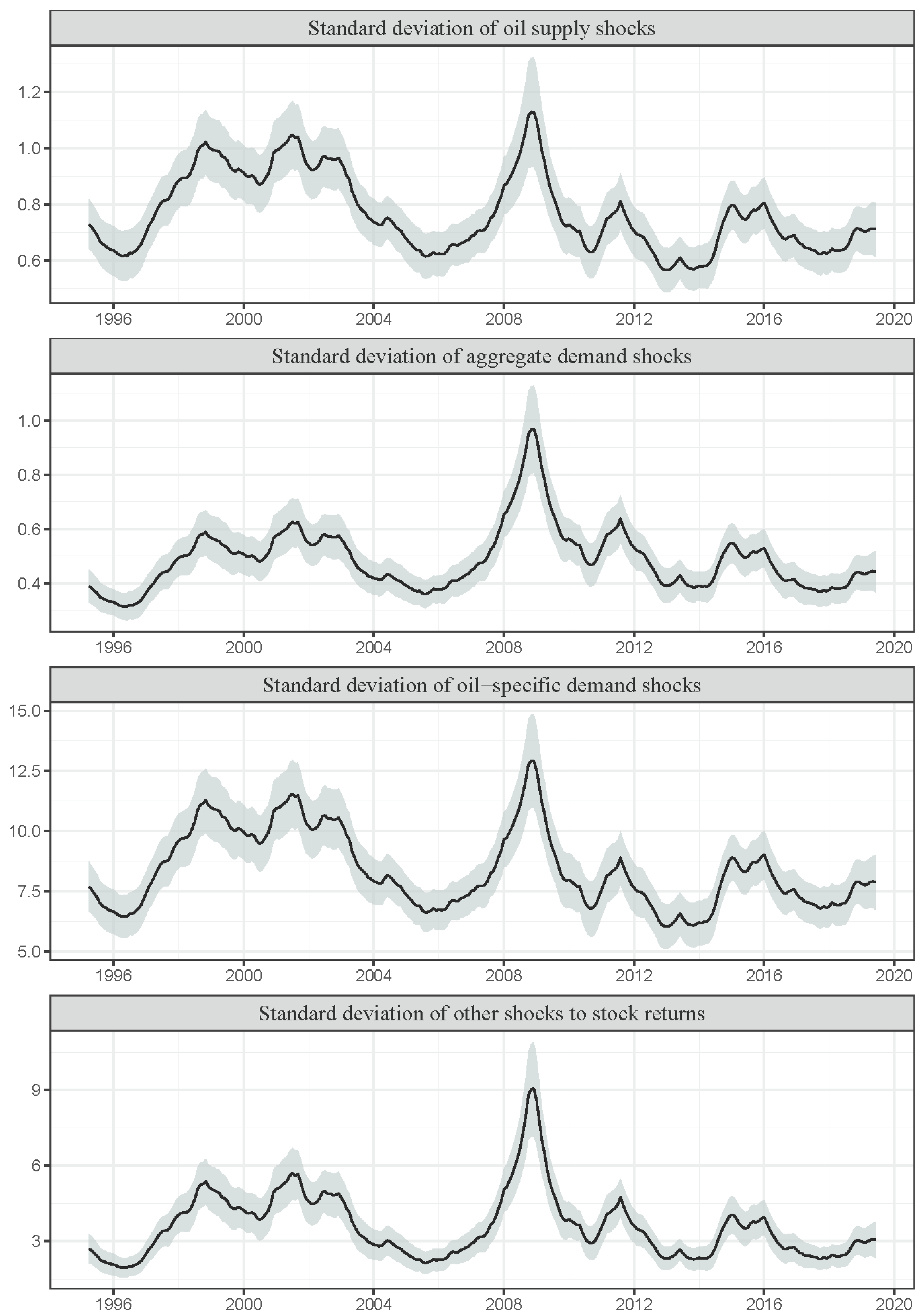
In this section, we analyze and discuss our research findings. Figure 2 shows the estimated time-varying standard deviations of the structural shocks obtained from the TVP-VAR model. The time-varying standard deviations underwent significant changes over time. They peaked in 2001–2002 and during the GFC. The standard deviation can be thought of as a measure of total risk. This measure is associated with various economic, financial and oil-market-specific events. Specifically, in 2001, hit by the Internet bubble collapse, the 9/11 terrorist attack, several accounting scandals, and recessionary monetary policy, the U.S. descended into a business cycle recession and experienced a stock market downswing. The U.S. economic and financial instabilities provoked by these events spilled over to the EU economy and financial markets, primarily France and Germany. Furthermore, the OPEC’s threat to cut oil production and its dispute with Russia contributed to greater oil market uncertainty.

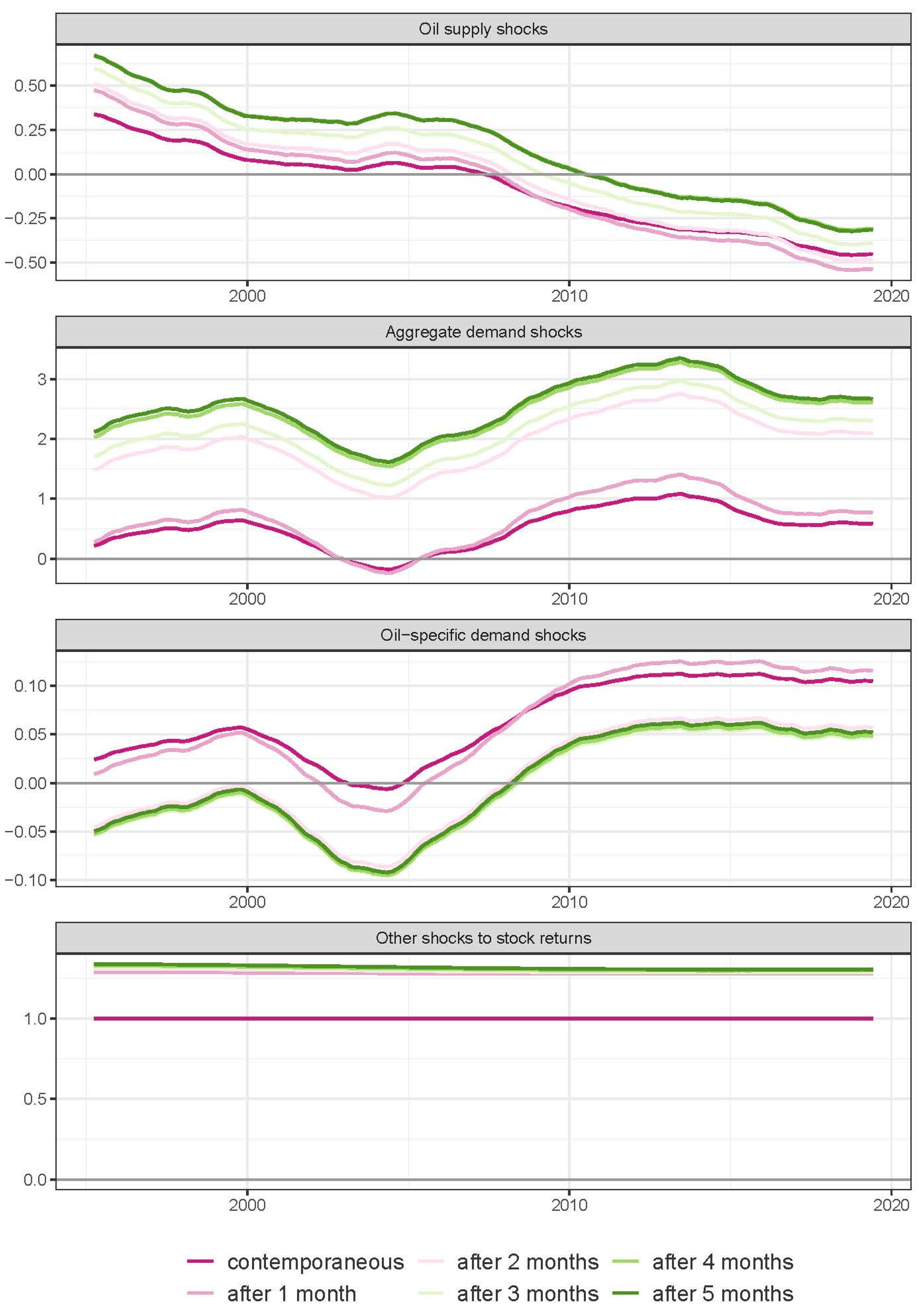
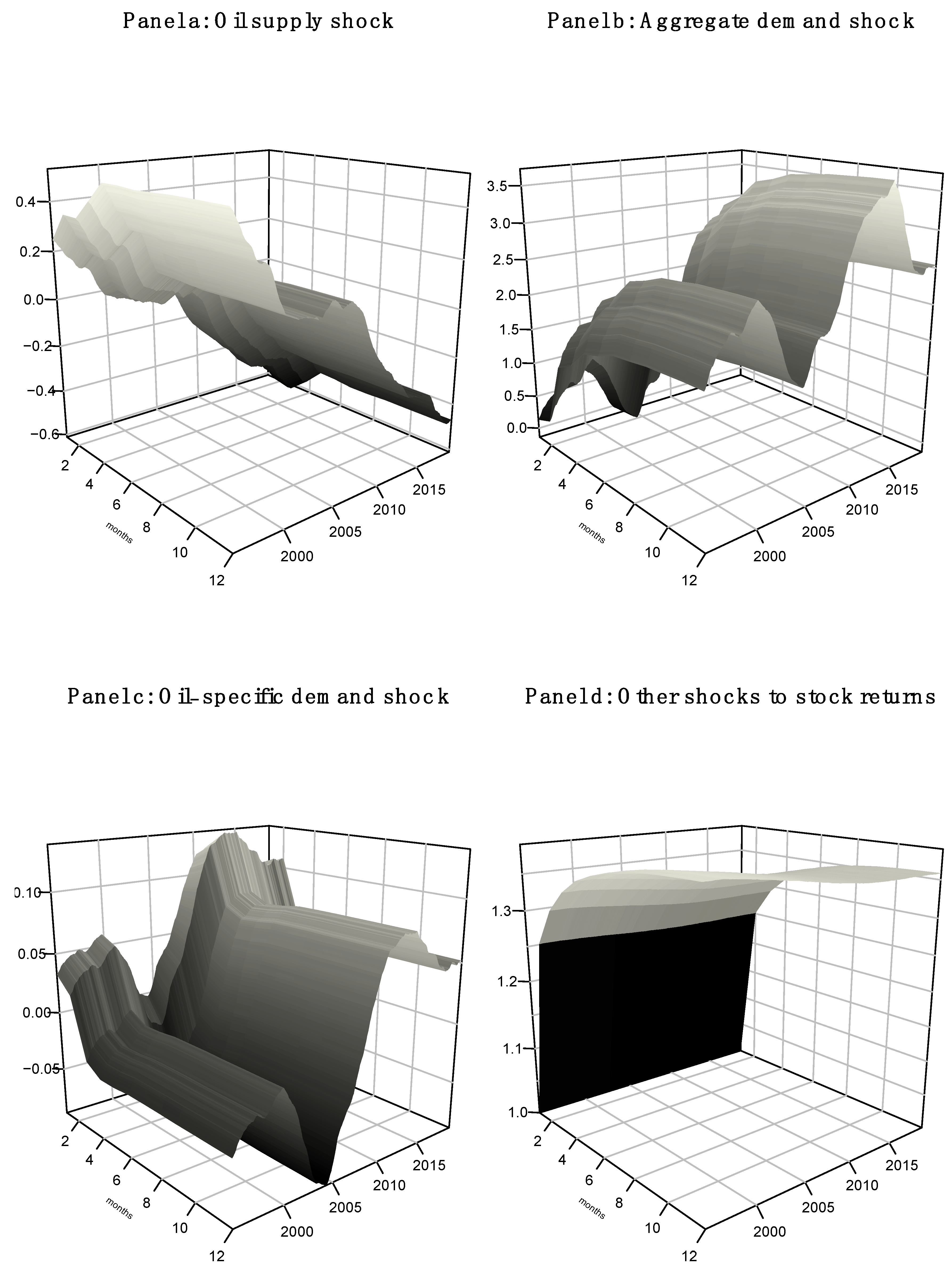
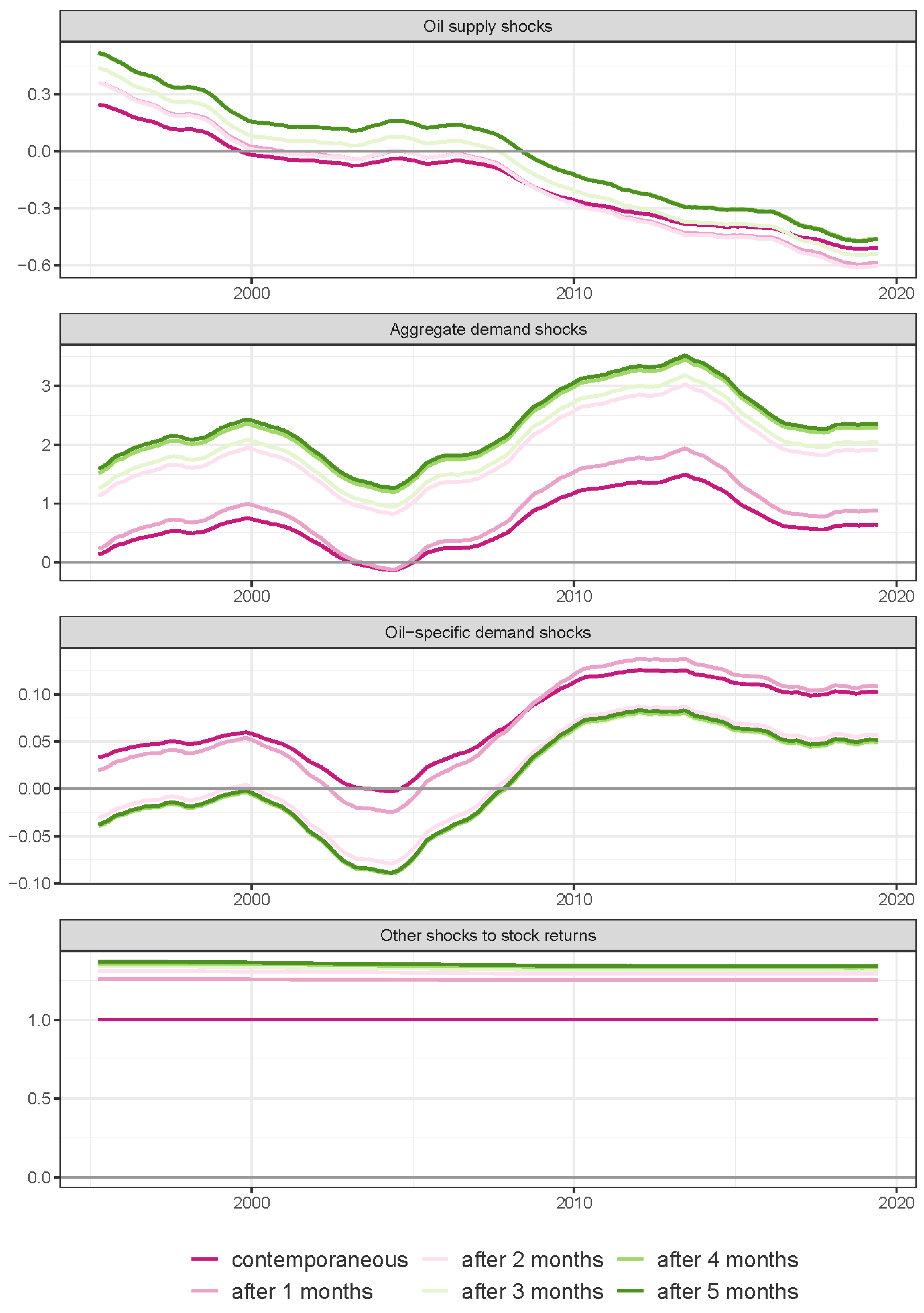
The accumulated impulse response functions are depicted in Figure 3, Figure 4, Figure 5 and Figure 6. The impulse response estimates the magnitude, sign and relevance of a contemporaneous and future change in the dependent variable when there is a contemporaneous one-unit shock to one of the dependent variables in the system, assuming that there are no further shocks in the future. The accumulated impulse response function accumulates the effects of a one-unit-sized shock over time. In particular, we consider the responses of aggregate stock returns to three structural oil shocks (an unexpected oil supply increase, an unanticipated aggregate demand expansion, and an unexpected increase in oil-specific demand), and a shock to real European stock returns that is not driven by oil shocks. For the convenience of the reader, we display in bidimensional graphs (Figure 3, Figure 4, Figure 5 and Figure 6) the time variation of the accumulated impulse responses contemporaneously and during the first five months after the shock, and we relegate the three-dimensional graphs to Appendix A. It is worth noting that, if the efficient market hypothesis holds, changes to an investor’s information contents, driven by oil shocks, are likely to be incorporated in the investor’s pricing and investment decisions with immediate effect. Any inefficiency in the stock market will translate into lagged effects of oil shocks on stock market returns. This justified our focus on the shorter-term impulse responses.

The accumulated impulse responses of returns on the Euro STOXX 50 stock market index show a significant variation over time and across the three structural oil shocks. The general picture that emerges from our estimation results is as follows. Consistent with Apergis and Miller (2009), Kilian and Park (2009), Basher et al. (2012) and Abhyankar et al. (2013), among others, our results show that each of the three structural shocks have a different impact on stock market returns. An in-depth examination is provided in three subsections. In Section 3.1, we scrutinize the time-varying effects of oil supply shocks (Figure 4). In Section 3.2, we study the time-varying effects of aggregate demand shocks (Figure 5). In Section 3.3, we analyze the time-varying effects of oil-specific demand shocks (Figure 6).

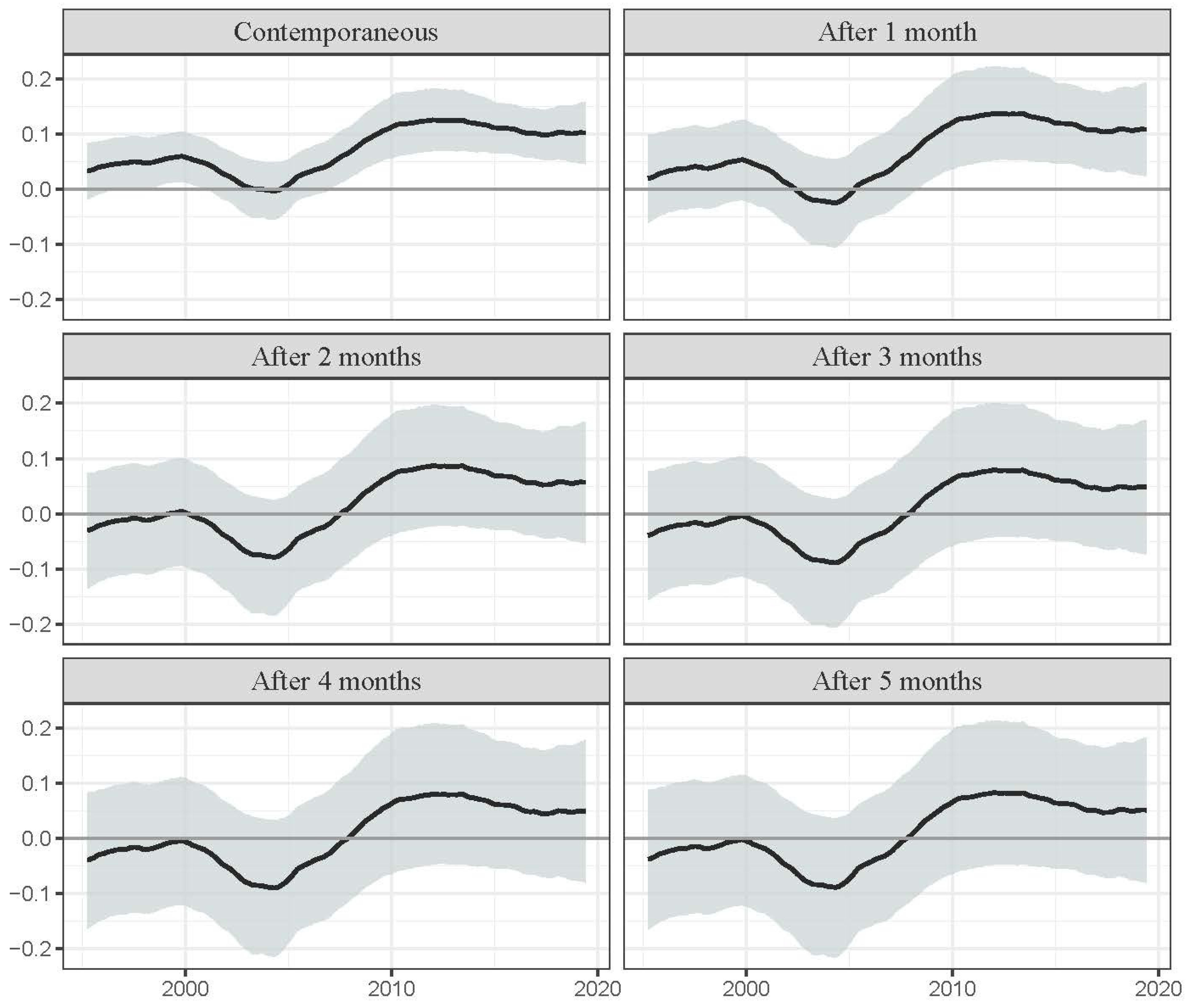
3.1. The Effects of the Oil Supply Shock

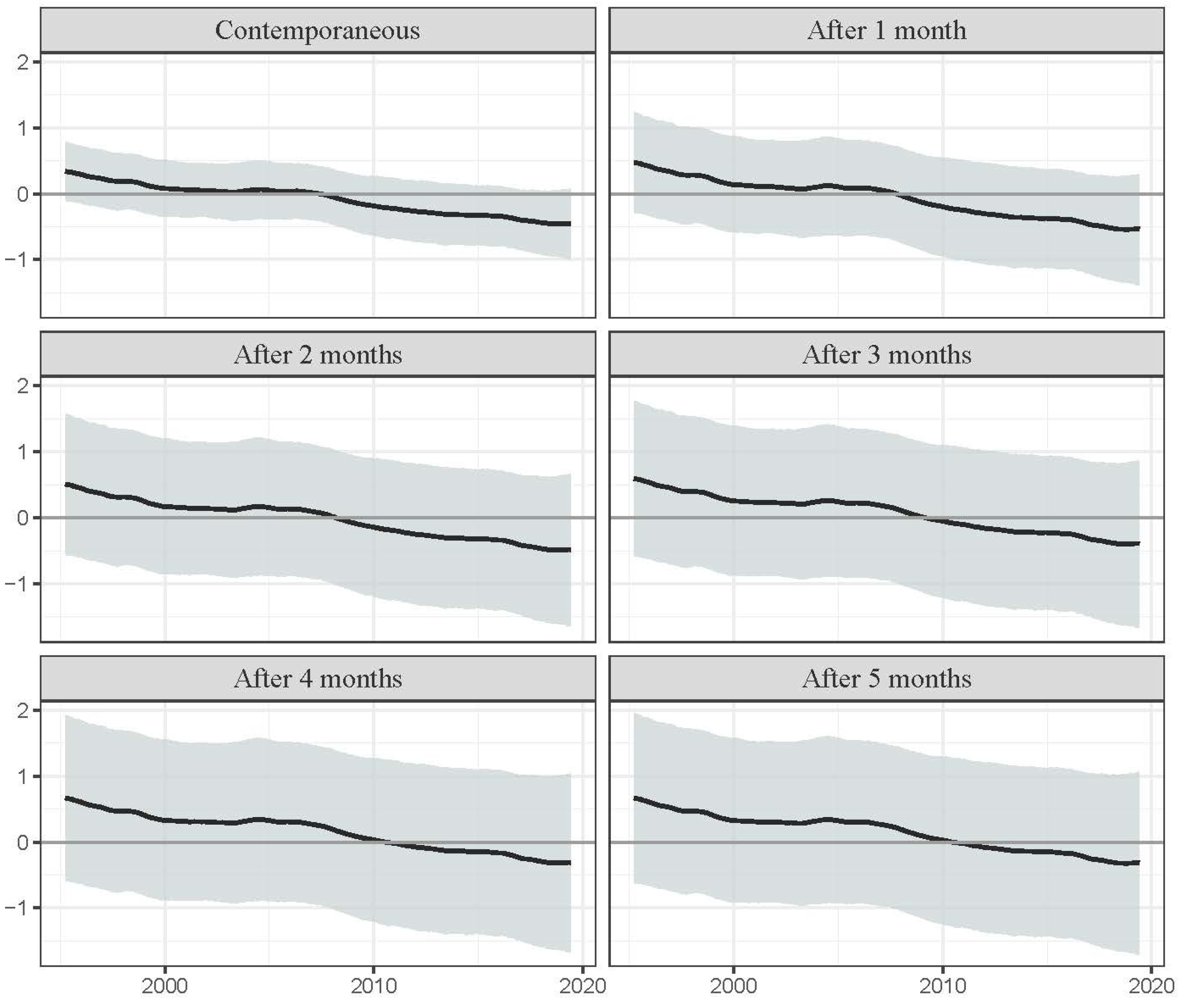
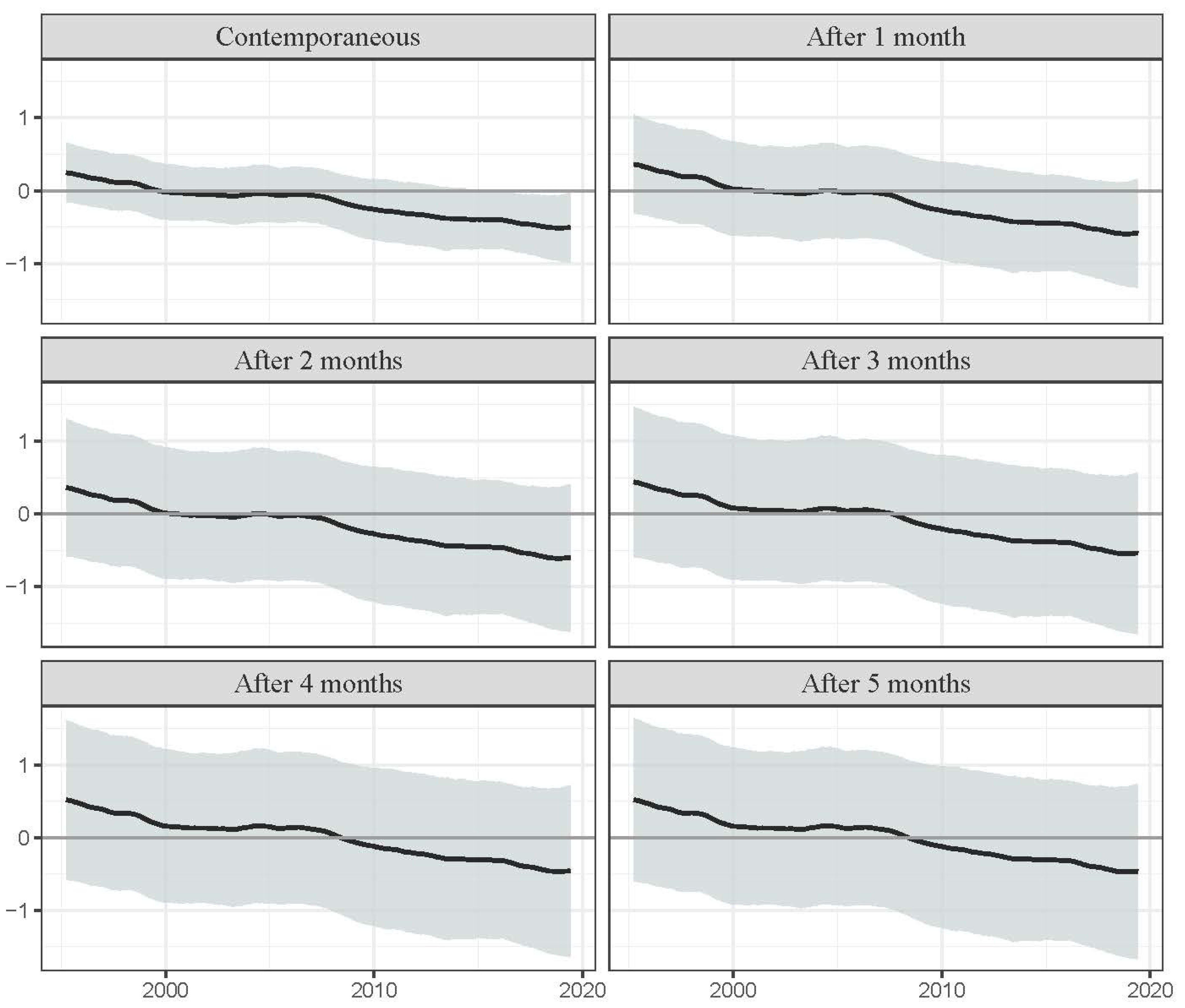
The structural oil supply shock was measured with a one-unit increase in the rate of growth of world crude oil production, and it was expected to have a positive effect on stock market returns. From a theoretical perspective, a positive supply-side shock is associated with an increase in world crude oil production and thus greater availability of oil, which generally has a negative effect on oil prices and, consequently, is perceived as positive news by stock market investors. A positive innovation to oil supply will have a negative effect on the oil price, which will reduce production costs of firms in oil-importing countries. As a result, profits of firms will increase and an appreciation in stock prices will be caused. By contrast, a negative supply-side shock will instigate a positive effect on the oil price. This is associated with a higher production cost, which reduces a company’s profits and induces investors to liquidate the company’s stock.

Our results (presented in Figure 4) show that an expansion of oil supply triggers a positive response in returns on the Euro STOXX 50 stock market index before 2008. The response in the following months after the shock becomes smaller in magnitude. The variation over time in the impulse response in stock market returns to a positive supply-side shock is partially consistent with Kilian and Park (2009), whose study centers on the U.S. economy, and with Wang et al. (2013), where the responses of oil-importing and oil-exporting countries are compared. Similar to Kang et al. (2015), our results indicate that the response declines over time, particular in the mid-2000s, before turning negative after 2008. This finding lends support to Güntner (2014) and Wang et al. (2013), who assert that oil supply shocks have become relatively weaker than aggregate demand shocks since the new millennium, and to Silvapulle et al. (2017), who document a declining effect of oil prices on stock prices. Moreover, the oil supply shocks appear to have weaker effects on the economy than aggregate demand shocks (Kilian 2009; Kilian and Park 2009). Nowadays, importing firms can effectively hedge against the risk associated with disruptions in crude oil production. Therefore, a negative supply-side shock does not necessarily trigger a rise in the oil price. Ready (2018) asserts that the stock market response to the oil supply shock depends on the industry of the oil-importing country, in which the company operates. Specifically, for industries which depend on consumption expenditure (i.e., consumer durables, consumer nondurables, and retail industries), the positive effect of supply-side shocks is stronger than for firms that operate in other industries.10 This finding receives support in Hamilton (2003), who asserts that oil prices act primarily on consumer expenditure rather than a direct effect from cost of imports. To the extent that the personal and household goods sectors become underweighted in the Euro STOXX 50 stock market index, the effect of supply-side shocks becomes weaker. Thus, even if a negative supply-side shock commands a rise in the oil price, investors may not necessarily unwind their investment positions in the stock market of an oil-importing country.

After the GFC, a positive supply-side shock triggered both a decline in the real oil price and lower European stock market returns. A plausible explanation for the observed negative stock market effect of a positive supply-side shock is that firms may substitute oil for alternative energy sources (Li et al. 2012). This explanation is founded on a theoretical assumption that a higher dependency of oil imports makes a country more vulnerable to oil price variations (Bergmann 2019). In this regard, Bergmann (2019) observes that the oil-to-energy share declined from 1970 to 2016 and finds that such a decline can act as a moderator of the economic and financial effects of oil price shocks.

After the GFC, the oil market has arguably become more financialized. As aforementioned, financialization manifests in a stronger comovement between the oil and stock markets. Therefore, the negative impulse response function in the post-GFC period is likely to be driven by a greater degree of financialization.

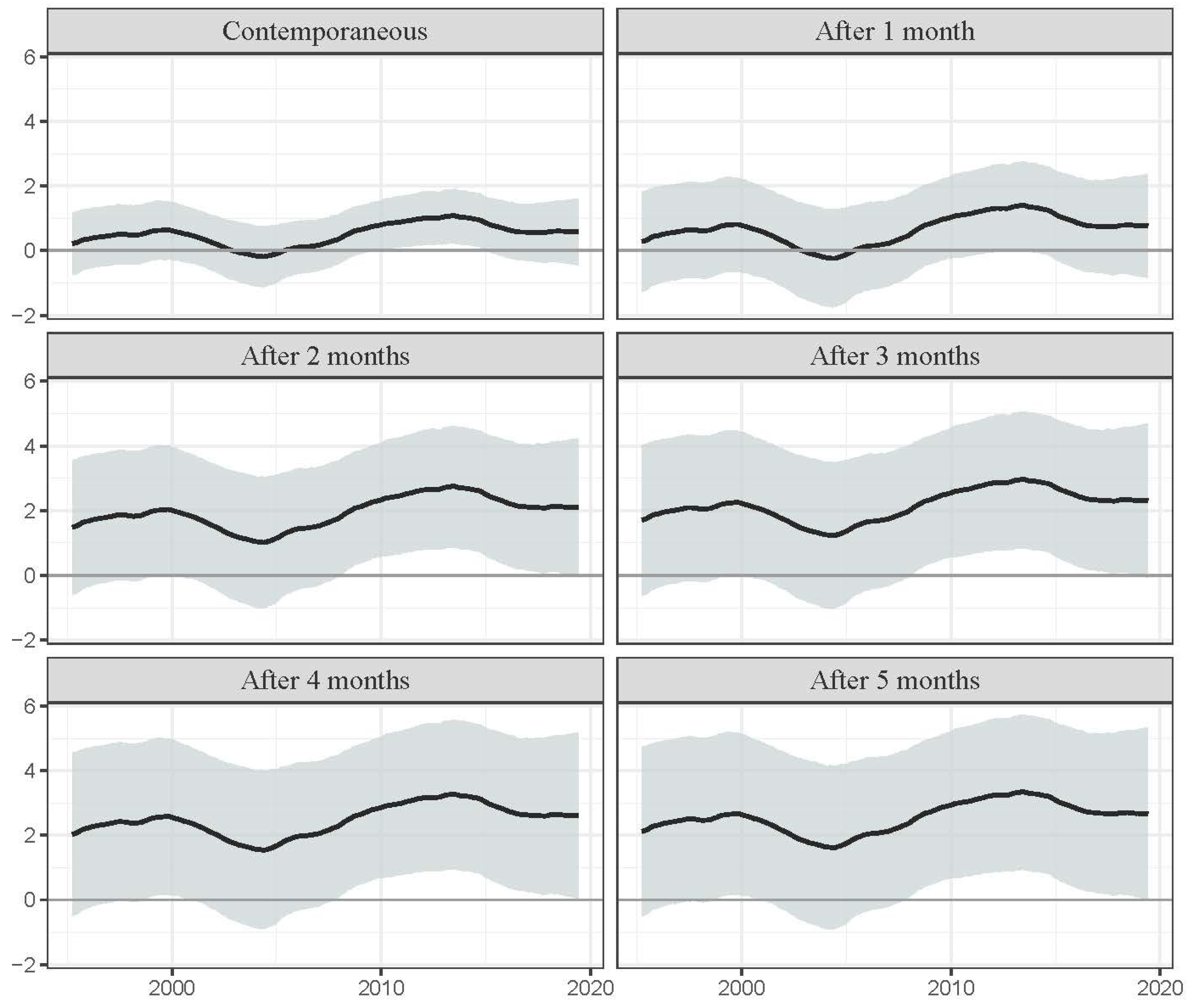
3.2. The Effects of the Aggregate Demand Shock

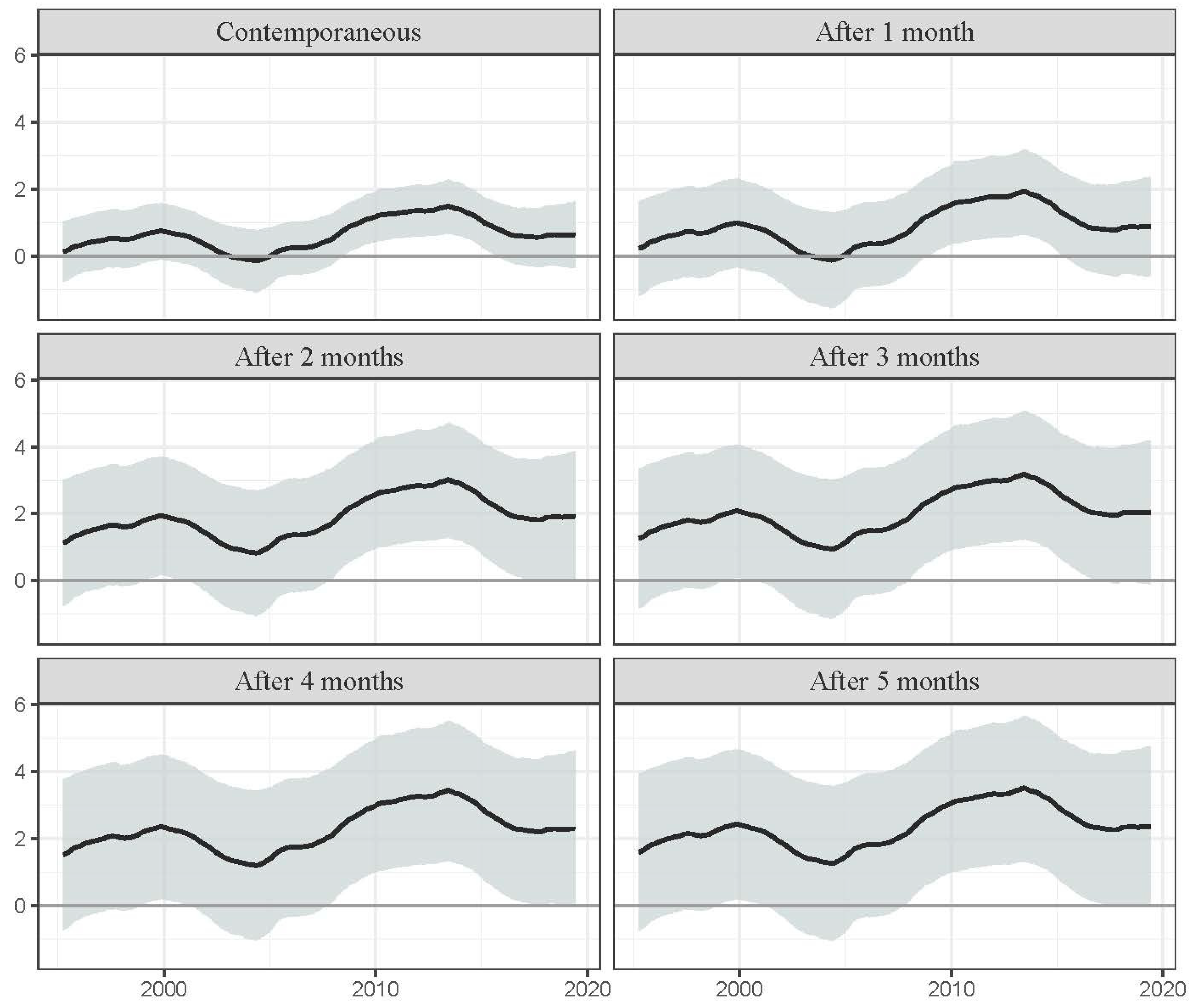
The structural positive aggregate demand shock was expected to have a positive effect on stock market returns. Turning to the effects of the aggregate demand shocks, we report the time-varying accumulated impulse response functions in Figure 5. In accordance with our ex-ante expectations, the global demand shock generally had a positive effect on returns on the Euro STOXX 50 stock market index. Our results are consistent with Kilian and Park (2009), who show that aggregate demand shocks exert a positive effect on stock market returns in the U.S., while Basher et al. (2012) provide similar evidence for emerging markets. A steep rise in consumption and investment spending in major emerging market economies, such as China and India, is regarded as a key driver of an aggregate demand shock. Wang et al. (2013) assert that, despite a series of supply-side shocks (e.g., the civil unrest in Venezuela in December 2002, the Iraq War in March 2003, the conflict in Nigeria in 2005, and Hurricanes Katrina and Rita in 2005, inter alia), the oil price since the millennium has been mainly driven by demand-side shocks. Along similar lines, variation in the oil price between mid-2003 and mid-2008 was attributed to recurrent positive aggregate demand shocks (Güntner 2014; Silvapulle et al. 2017) and shocks to the demand for industrial commodities (Kilian and Park 2009; Kilian and Hicks 2013). For instance, Kilian and Hicks (2013) assert that these positive shocks signal unexpectedly high growth in emerging Asian economies that drives the global business cycle. Kilian and Murphy (2014) and Kilian and Lee (2014) second this view but assert that the observed increase in the oil price in the abovementioned period was not driven by speculative demand shocks. A positive innovation in the global business cycle may lead to a rise in returns in both oil and stock markets, after controlling for crude oil production. This generates a positive comovement between returns in oil and stock markets. Therefore, in a global business cycle expansion, an aggregate demand shock is perceived as good news by the stock market, since it triggers an upward revision in future expected dividends of firms. This positive comovement may mitigate any negative relation between returns in oil and stock markets (Moya-Martínez et al. 2014; Le and Chang 2015).

Notably, the impulse response function does not show a monotonic pattern. The contemporaneous response experienced a positive trend between 1995 and 2000, which was reversed thereafter. The response briefly descended into negative values in 2003, but became positive again in 2005. Although the negative aggregate demand effect generally does not agree with our ex-ante expectations, we should not lose sight of the fact that a positive aggregate demand shock, in addition to causing the abovementioned direct stimulating short-run effect, also triggers a longer-run indirect growth-retarding effect (Kilian 2009). The indirect negative effect is conducive to higher oil prices, and it translates into a higher consumption and production cost in the long run, when the direct effect wears out. Thus, one reason behind the negative aggregate demand effect could be driven by the indirect negative effect from 2003 to 2005. Moreover, an aggregate demand shock exerts a positive effect in a high-volatility regime, although not in a low-volatility regime (Zhu et al. 2017). From 2005 to 2013/14 the response displayed a continuous growth. This period was marked by stable oil prices (2010–2014). It peaked in 2014, descended during 2014–2016, and plateaued in 2016–17.

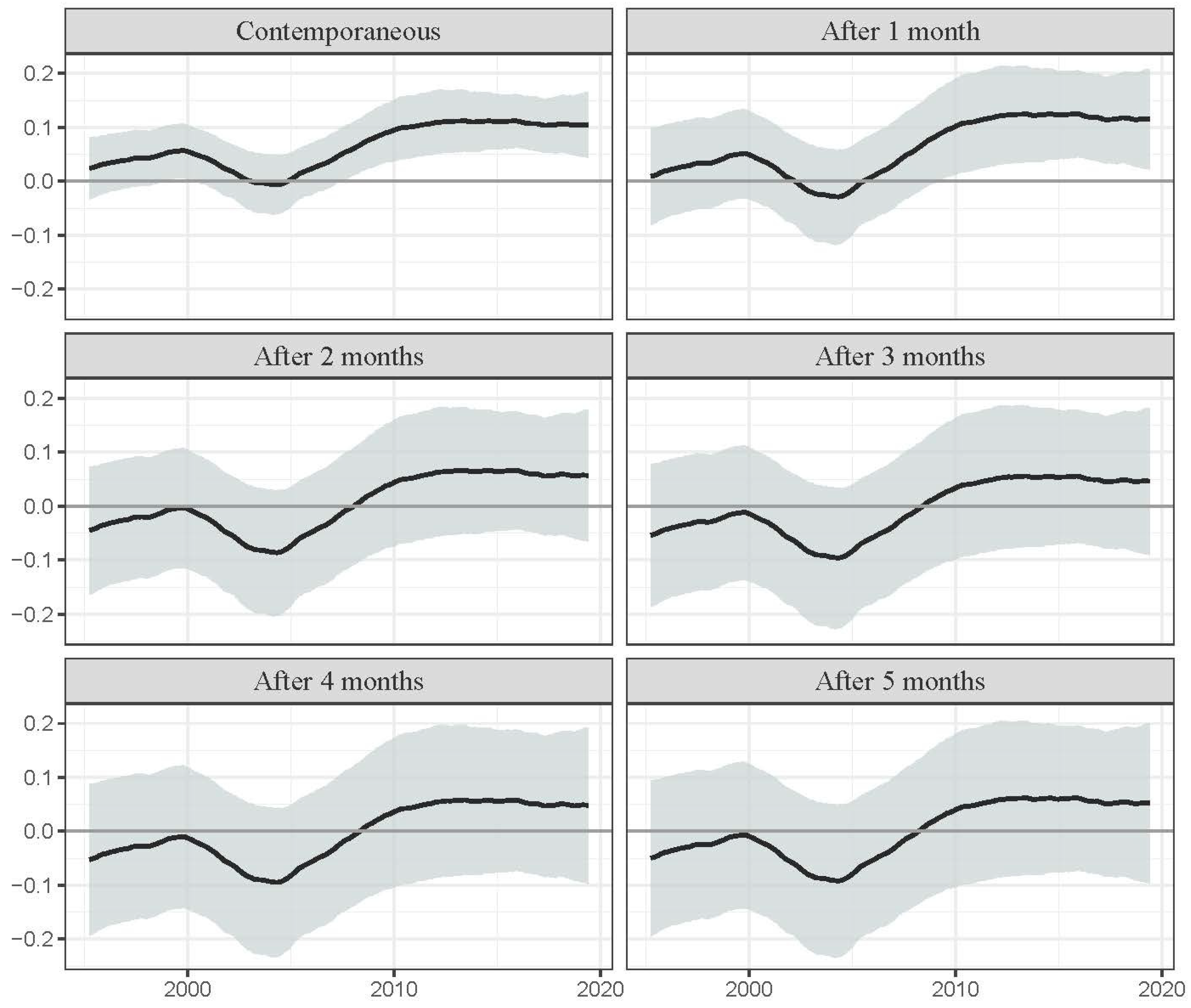
3.3. The Effects of the Oil-Specific Demand Shock

The structural oil-specific demand shock tries to capture the change in precautionary demand for crude oil that arises due to heightened uncertainty about shortfalls of expected supply relative to expected demand for crude oil (Sim and Zhou 2015). Whilst the structural aggregate demand shock can affect the demand for other commodities and thus global economic activity, the effects of the oil-specific demand shock are confined to the crude oil market. Specifically, this shock will influence the demand for crude oil inventory holdings as a way of ensuring against any unanticipated interruption in oil supplies, which will have an effect on oil price (Sim and Zhou 2015). Increased uncertainty about shortfalls of expected relative supply of crude oil will translate into heightened uncertainty surrounding future production costs and thus future profits of firms. In episodes of heightened uncertainty, investors will demand a higher risk premium and a higher expected return on stock market investments. A higher expected return can be attained if the contemporaneous stock price decreases sufficiently for a given future expected stock price. Therefore, we expect that a positive oil-specific shock exerts a negative influence on returns on the Euro STOXX 50 stock market index. Results, depicted in Figure 6, are indicative of a positive stock market response 4–5 months after the shock in the pre-GFC period. During and after the GFC, contrary to our ex-ante expectations, we find that oil-specific demand shocks generally had a positive impact on stock market returns.

It is worth mentioning that an oil-specific demand shock may also convey news about speculative demand for oil inventories (Kilian and Murphy 2014; Kilian and Lee 2014). Speculative trades thrive in periods of heightened uncertainty about shortfalls in future oil supply. A speculative demand shock will command deviations of the oil price from oil market fundamentals. Therefore, the oil-specific demand shock can be decomposed into two components. The first component is referred to the precautionary demand shock, which conveys information of hedging activities of traders in the crude market. For instance, in Alquist and Kilian (2010), the general equilibrium model implies that oil importers insure against uncertainty about stochastic oil endowments by holding above-ground oil inventories or buying oil futures. The second component is the speculative demand shock, which arises due to financial speculation that is unrelated to economic or oil market fundamentals. On the one hand, higher precautionary demand should lead to a negative effect on the rate of return on the Euro STOXX 50 stock market index. On the other hand, higher speculative demand is likely to increase the degree of association between returns in oil and stock markets, since it can be regarded as a precursor for greater financialization of the oil. Therefore, if the precautionary demand shock dominates, we would expect a negative effect on return on the stock market. By contrast, if the speculative demand shock dominates, we would expect a positive effect of the oil-specific demand shock. A positive (negative) speculative demand shock leads to an accumulation of oil inventories and an increase (decrease) in the price of crude oil. In this regard, Kilian and Murphy (2014) find that shifts in speculative demand significantly contributed to changes in the oil price in 1990 and 2002–2003. Concretely, they argue that the Venezuelan oil supply crisis in 2002 and the anticipation of the 2003 Iraq War coincided with an increase in speculative demand, when the stock market effect of an oil-specific demand shock was positive. Further, Kilian and Lee (2014) find that the crude oil price increased between USD $5 and USD $14 from March to July 2008 due to a speculative demand shock. However, the rise in the oil price experienced a sharp reversal thereafter, which lasted until 2009, and was driven mainly by a negative aggregate demand shock. Nevertheless, in the period from 2009 to 2012, the effect of the oil-specific demand shock remained positive, which partly lends support to Kilian and Lee (2014). For instance, they report that the Libyan revolution in February 2011 and the tension with Iran in 2012 affected the oil price by shifting speculative demand for crude oil inventory holdings.

Overall, the behavior of commodities experienced structural shifts between 2004 and the GFC (e.g., Tang and Xiong 2012). Prominent among the alleged causes for these shifts is financialization, which is expected to generate a positive comovement between returns in oil and stock markets, and can be regarded as a speculative demand shock. For instance, flows into commodity investments began to rise at an unprecedented rate in 2003, and are reported to have increased from USD $15 billion in 2003 to USD $250 billion in 2009 (Irwin and Sanders 2011; Adams and Glück 2015, inter alia). These investments did not materialize until the outbreak of the GFC in September 2008 (Adams and Glück 2015), when investor confidence in both oil and stock markets became undermined by heightened uncertainty (Kim et al. 2019). In the months following the Lehman collapse in September 2008, the prices of most tradable assets experienced pronounced declines within the same day (Adams and Glück 2015), which can be attributed to liquidity and risk spillovers from stock to commodity markets (Brunnermeier and Pedersen 2009). Specifically, Adams and Glück (2015) show that liquidity and risk spillovers manifested in a simultaneous disposition of commodities and stocks, and remained persistently high until the end of 2013. The bearish stance marked by the widespread liquidation of assets in both oil and stock markets generated a positive financial effect of the oil-specific demand shock. The period from June 2014 to August 2015 was particularly bearish for the oil market, as the WTI oil price fell from USD $105 in June 2014 to only USD $43 in August 2015.

As a robustness check, we have estimated the TVP-VAR model described in the main text using the real return on the STOXX Europe 600 stock market index instead of the real return on the Euro STOXX 50 stock market index. We can observe that the results are very similar. Results are reported and discussed in Appendix A and Supplementary Material.

4. Conclusions

In this paper, we used a TVP-VAR model to examine the effects of oil shocks on the European stock market. Following Kilian (2009), we disentangled three structural oil shocks: the supply-side shock, the aggregate demand shock, and the oil-specific demand shock. Subsequently, we scrutinized the time-varying impulse response functions of returns on the Euro STOXX 50 stock market index to the three oil shocks. Our research findings are as follows. First, we found that an unexpected increase in oil supply exerted a positive effect on returns on the Euro STOXX 50 stock market index until the GFC. After the GFC, the impulse response showed a declining trend before turning negative. This is in agreement with the related literature, which demonstrates that in the new millennium, variation over time in oil prices is predominantly driven by demand-side shocks. Second, we found that an unanticipated expansion in aggregate demand led to an appreciation of the Euro STOXX 50 stock market index. However, the short-term impulse response function of the stock market index experienced large swings over the sample period. It followed a positive trend until around 2000, when the trend was reversed. The impulse response function was then declining over time before descending into negative values in 2004. From 2004, the impulse response function remained positive, and showed a positive trend until 2013. Third, the contemporaneous effect of an unexpected increase in oil-specific demand was positive, whereas the lagged effect was negative. The sign of the impulse response was determined by the balance of precautionary and speculative motives of traders. The former predicts a negative effect on the stock market index, whereas the latter predicts a positive effect, which is driven by financialization of the oil market. Exhaustive scrutiny of the impulse response function indicated that, in the pre-GFC period, the oil-specific demand was determined by the precautionary motive, whereas after the GFC, the effect of the oil-specific demand shock was indicative of speculative behavior.

In response to our first research question, we documented that the stock market effects of the three oil shocks varied in sign. Our research findings provided a positive answer to the second research question; indeed, the response of the European stock market to the three oil shocks underwent considerable changes over time. Third, as aforementioned, the signs of the responses of the European stock market to supply-side, aggregate-demand and oil-specific-demand shocks were found to be time- and episode-specific.

Our research findings are of the utmost importance for oil and stock market analysts, investors, financial regulators, and policy makers. For instance, we show that stock market investors need to be aware that investment opportunities vary over time and respond to changes in oil prices. Importantly, whether an oil shock can be regarded as positive or negative news for the stock market is determined by its origin. In this regard, we assert that when the oil price is driven by aggregate or speculative demand shocks, the Euro STOXX 50 stock market index appreciates. By contrast, when the oil price changes in response to a precautionary demand shock, the stock market index depreciates. Further, when a supply-side shock commands a change in the oil price, the response of the stock market index is likely to be inconclusive. Both the oil and stock markets need to be monitored by financial regulators and policy makers, since abrupt changes in the oil market can compromise financial stability.

Admittedly, additional information and further identifying assumptions or restrictions are required to disentangle precautionary and speculative demand shocks, which constitute key limitations of our research. Therefore, these limitations could translate into a future research avenue. Specifically, future research could incorporate inventories in the modelling of the crude oil market as a measure of crude market liquidity and a driver of the wedge between hedging and speculative activities. This research would shed further light on the determinants of the time-varying impulse response functions of the stock market index, as well as stock market volatility. Furthermore, future research could explore the time-varying effects of oil price shocks on sovereign bond returns. In this regard, and differently to Filippidis et al. (2020), who examined the time-varying correlations of the supply-side, aggregate-demand and oil-specific demand shocks with the 10-year sovereign bond yield spread of core and periphery countries in the European Monetary Union, scholars could evaluate the causal effects of the three shocks on European sovereign bond yields using a TVP-VAR model.

References

1. Abhyankar, Abhay, Bing Xu, and Jiayue Wang. 2013. Oil Price Shocks and the Stock Market: Evidence from Japan. The Energy Journal 34: 199–222. [Google Scholar] [CrossRef]
2. Adams, Zeno, and Thorsten Glück. 2015. Financialization in commodity markets: A passing trend or the new normal? Journal of Banking & Finance 60: 93–111. [Google Scholar] [CrossRef] [Green Version]
3. Aloui, Riadh, Shawkat Hammoudeh, and Duc Khuong Nguyen. 2013. A time-varying copula approach to oil and stock market dependence: The case of transition economies. Energy Economics 39: 208–21. [Google Scholar] [CrossRef]
4. Alquist, Ron, and Lutz Kilian. 2010. What do we learn from the price of crude oil futures? Journal of Applied Econometrics 25: 539–73. [Google Scholar] [CrossRef] [Green Version]
5. Anzuini, Alessio, Patrizio Pagano, and Massimiliano Pisani. 2015. Macroeconomic Effects of Precautionary Demand for Oil. Journal of Applied Econometrics 30: 968–86. [Google Scholar] [CrossRef]
6. Apergis, Nicholas, and Stephen M. Miller. 2009. Do structural oil-market shocks affect stock prices? Energy Economics 31: 569–75. [Google Scholar] [CrossRef] [Green Version]
7. Arouri, Mohamed El Hedi. 2011. Does crude oil move stock markets in Europe? A sector investigation. Economic Modelling 28: 1716–25. [Google Scholar] [CrossRef]
8. Barberis, Nicholas, Andrei Shleifer, and Robert Vishny. 1998. A model of investor sentiment. Journal of Financial Economics 9: 307–43. [Google Scholar] [CrossRef]
9. Basher, Syed Abul, Alfred A. Haug, and Perry Sadorsky. 2012. Oil prices, exchange rates and emerging stock markets. Energy Economics 34: 227–40. [Google Scholar] [CrossRef] [Green Version]
10. Basher, Syed Abul, Alfred A. Haug, and Perry Sadorsky. 2018. The impact of oil-market shocks on stock returns in major oil-exporting countries. Journal of International Money and Finance 86: 264–80. [Google Scholar] [CrossRef]
11. Baumeister, Christiane, and James D. Hamilton. 2019. Structural Interpretation of Vector Autoregressions with Incomplete Identification: Revisiting the Role of Oil Supply and Demand Shocks. The American Economic Review 109: 1873–910. [Google Scholar] [CrossRef] [Green Version]
12. Bergmann, Philip. 2019. Oil price shocks and GDP growth: Do energy shares amplify causal effects? Energy Economics 80: 1010–40. [Google Scholar] [CrossRef] [Green Version]
13. Bernanke, Ben S., Mark Gertler, Mark Watson, Christopher A. Sims, and Benjamin M. Friedman. 1997. Systematic Monetary Policy and the Effects of Oil Price Shocks. Brookings Papers on Economic Activity 1997: 91. [Google Scholar] [CrossRef] [Green Version]
14. Bjørnland, Hilde C. 2009. Oil Price Shocks and Stock Market Booms in an Oil Exporting Country. Scottish Journal of Political Economy 56: 232–54. [Google Scholar] [CrossRef] [Green Version]
15. Brunnermeier, Markus K., and Lasse Heje Pedersen. 2009. Market Liquidity and Funding Liquidity. The Review of Financial Studies 22: 2201–38. [Google Scholar] [CrossRef] [Green Version]
16. Ciner, Cetin. 2001. Energy shocks and financial markets: Nonlinear linkages. Studies in Nonlinear Dynamics and Econometrics 5: 203–12. [Google Scholar] [CrossRef]
17. Ciner, Cetin. 2013. Oil and stock returns: Frequency domain evidence. Journal of International Financial Markets, Institutions and Money 23: 1–11. [Google Scholar] [CrossRef]
18. Ciner, Cetin, Constantin Gurdgiev, and Brian M. Lucey. 2013. Hedges and safe havens: An examination of stocks, bonds, gold, oil and exchange rates. International Review of Financial Analysis 29: 202–11. [Google Scholar] [CrossRef]
19. Cont, Rama. 2001. Empirical properties of asset returns: Stylized facts and statistical issues. Quantitative Finance 1: 223–36. [Google Scholar]
20. Degiannakis, Stavros, George Filis, and Renatas Kizys. 2014. The Effects of Oil Price Shocks on Stock Market Volatility: Evidence from European Data. The Energy Journal 35: 35–56. [Google Scholar] [CrossRef] [Green Version]
21. Del Negro, Marco, and Giorgio E. Primiceri. 2015. Time Varying Structural Vector Autoregressions and Monetary Policy: A Corrigendum. The Review of Economic Studies 82: 1342–45. [Google Scholar] [CrossRef] [Green Version]
22. Filippidis, Michail, George Filis, and Renatas Kizys. 2020. Oil price shocks and EMU sovereign yield spreads. Energy Economics 86: 104656. [Google Scholar] [CrossRef]
23. Filis, George, Stavros Degiannakis, and Christos Floros. 2011. Dynamic correlation between stock market and oil prices: The case of oil-importing and oil-exporting countries. International Review of Financial Analysis 20: 152–64. [Google Scholar] [CrossRef]
24. Güntner, Jochen H. F. 2014. How do International Stock Markets Respond to Oil Demand and Supply Shocks? Macroeconomic Dynamics 18: 1657–82. [Google Scholar] [CrossRef] [Green Version]
25. Hamilton, James D. 2003. What is an oil shock? Journal of Econometrics 113: 363–98. [Google Scholar] [CrossRef]
26. Hamilton, James D. 2021. Measuring global economic activity. Journal of Applied Econometrics 36: 293–303. [Google Scholar] [CrossRef]
27. Huang, Roger D., Ronald W. Masulis, and Hans R. Stoll. 1996. Energy shocks and financial markets. The Journal of Futures Markets 16: 1–27. [Google Scholar] [CrossRef]
28. Irwin, Scott H., and Dwight R. Sanders. 2011. Index funds, financialization, and commodity futures markets. Applied Economic Perspectives and Policy 33: 1–31. [Google Scholar] [CrossRef] [Green Version]
29. Jiménez-Rodríguez, Rebeca. 2015. Oil price shocks and stock markets: Testing for non-linearity. Empirical Economics 48: 1079–102. [Google Scholar] [CrossRef]
30. Jones, Charles M., and Gautam Kaul. 1996. Oil and the stock markets. Journal of Finance 51: 463–91. [Google Scholar] [CrossRef]
31. Kang, Wensheng, Ronald A. Ratti, and Kyung Hwan Yoon. 2015. Time-varying effect of oil market shocks on the stock market. Journal of Banking & Finance 61: S150–S163. [Google Scholar] [CrossRef] [Green Version]
32. Kilian, Lutz. 2008. A Comparison of the Effects of Exogenous Oil Supply Shocks on Output and Inflation in the G7 Countries. Journal of the European Economic Association 6: 78–121. [Google Scholar] [CrossRef] [Green Version]
33. Kilian, Lutz. 2009. Not All Oil Price Shocks Are Alike: Disentangling Demand and Supply Shocks in the Crude Oil Market. The American Economic Review 99: 1053–69. [Google Scholar] [CrossRef] [Green Version]
34. Kilian, Lutz. 2019. Measuring global real economic activity: Do recent critiques hold up to scrutiny? Economics Letters 178: 106–10. [Google Scholar] [CrossRef] [Green Version]
35. Kilian, Lutz, and Bruce Hicks. 2013. Did Unexpectedly Strong Economic Growth Cause the Oil Price Shock of 2003–2008? Journal of Forecasting 32: 385–94. [Google Scholar] [CrossRef] [Green Version]
36. Kilian, Lutz, and Cheolbeom Park. 2009. The impact of oil price shocks on the U.S. stock market. International Economic Review 50: 1267–87. [Google Scholar] [CrossRef]
37. Kilian, Lutz, and Daniel P. Murphy. 2014. The role of inventories and speculative trading in the global market for crude oil. Journal of Applied Econometrics 29: 454–78. [Google Scholar] [CrossRef]
38. Kilian, Lutz, and Helmut Lütkepohl. 2017. Identification by Short-Run Restrictions. In Structural Vector Autoregressive Analysis (Themes in Modern Econometrics). Cambridge: Cambridge University Press, pp. 216–40. [Google Scholar]
39. Kilian, Lutz, and Thomas K. Lee. 2014. Quantifying the speculative component in the real price of oil: The role of global oil inventories. Journal of International Money and Finance 42: 71–87. [Google Scholar] [CrossRef]
40. Kim, Jae H., Lutfur Rahman, and Abul Shamsuddin. 2019. Can energy prices predict stock returns? An extreme bounds analysis. Energy Economics 81: 822–34. [Google Scholar] [CrossRef]
41. Le, Thai-Ha, and Youngho Chang. 2015. Effects of oil price shocks on the stock market performance: Do nature of shocks and economies matter? Energy Economics 51: 261–74. [Google Scholar] [CrossRef]
42. Li, Su-Fang, Hui-Ming Zhu, and Keming Yu. 2012. Oil prices and stock market in China: A sector analysis using panel cointegration with multiple breaks. Energy Economics 34: 1951–58. [Google Scholar] [CrossRef]
43. Miller, J. Isaac, and Ronald A. Ratti. 2009. Crude oil and stock markets: Stability, instability, and bubles. Energy Economics 31: 559–68. [Google Scholar] [CrossRef] [Green Version]
44. Mollick, André Varella, and Tibebe Abebe Assefa. 2013. U.S. stock returns and oil prices: The tale from daily data and the 2008–9 financial crisis. Energy Economics 36: 1–18. [Google Scholar] [CrossRef]
45. Moya-Martínez, Pablo, Román Ferrer-Lapeña, and Francisco Escribano-Sotos. 2014. Oil price risk in the Spanish stock market: An industry perspective. Economic Modelling 37: 280–90. [Google Scholar] [CrossRef]
46. Narayan, Paresh Kumar, and Susan Sunila Sharma. 2011. New evidence on oil price and firm returns. Journal of Banking & Finance 35: 3253–62. [Google Scholar] [CrossRef]
47. Papapetrou, Evangelia. 2001. Oil price shocks, stock market, economic activity and employment in Greece. Energy Economics 23: 511–32. [Google Scholar] [CrossRef]
48. Park, Jungwook, and Ronald A. Ratti. 2008. Oil price shocks and stock markets in the U.S. and 13 European countries. Energy Economics 30: 2587–608. [Google Scholar] [CrossRef]
49. Primiceri, Giorgio E. 2005. Time Varying Structural Vector Autoregressions and Monetary Policy. The Review of Economic Studies 72: 821–52. [Google Scholar] [CrossRef]
50. Ramos, Sofia B., and Helena Veiga. 2013. Oil price asymmetric effects: Answering the puzzle in international stock markets. Energy Economics 38: 136–45. [Google Scholar] [CrossRef] [Green Version]
51. Ready, Robert C. 2018. Oil prices and the stock market. Review of Finance 22: 155–76. [Google Scholar] [CrossRef]
52. Reboredo, Juan C., and Miguel A. Rivera-Castro. 2014. Wavelet-based evidence of the impact of oil prices on stock returns. International Review of Economics & Finance 29: 145–76. [Google Scholar] [CrossRef]
53. Sadorsky, Perry. 1999. Oil price shocks and stock market activity. Energy Economics 21: 449–69. [Google Scholar] [CrossRef]
54. Sadorsky, Perry. 2014. Modeling volatility and correlations between emerging market stock prices and the prices of copper, oil and wheat. Energy Economics 43: 72–81. [Google Scholar] [CrossRef]
55. Silvapulle, Param, Russell Smyth, Xibin Zhang, and Jean-Pierre Fenech. 2017. Nonparametric panel data model for crude oil and stock market prices in net oil importing countries. Energy Economics 67: 255–67. [Google Scholar] [CrossRef]
56. Sim, Nicholas, and Hongtao Zhou. 2015. Oil prices, US stock return, and the dependence between their quantiles. Journal of Banking & Finance 55: 1–8. [Google Scholar]
57. Soytas, Ugur, Ramazan Sari, Shawkat Hammoudeh, and Erk Hacihasanoglu. 2009. World oil prices, precious metal prices and macroeconomy in Turkey. Energy Policy 37: 5557–66. [Google Scholar]
58. Tang, Ke, and Wei Xiong. 2012. Index Investment and the Financialization of Commodities. Cfa Institute Magazine 68: 54–74. [Google Scholar] [CrossRef]
59. Tsai, Chun-Li. 2015. How do U.S. stock returns respond differently to oil price shocks pre-crisis, within the financial crisis, and post-crisis? Energy Economics 50: 47–62. [Google Scholar] [CrossRef]
60. UNCTAD. 2009. Trade and Development Report 2009. Geneva: UNCTAD. [Google Scholar]
61. Wang, Yudong, Chongfeng Wu, and Li Yang. 2013. Oil price shocks and stock market activities: Evidence from oil-importing and oil-exporting countries. Journal of Comparative Economics 41: 1220–39. [Google Scholar] [CrossRef]
62. Zhu, Huiming, Xianfang Su, Wanhai You, and Yinghua Ren. 2017. Asymmetric effects of oil price shocks on stock returns: Evidence from a two-stage Markov regime-switching approach. Applied Economics 49: 2491–507. [Google Scholar] [CrossRef]
Figure 1. Evolution of returns. Note: This figure shows the evolution of returns on world oil production, world industrial production, oil prices and the Euro STOXX 50 stock market index, respectively.
Jrfm 16 00174 g001
Figure 2. Standard deviations of structural shocks. Note: This figure presents the posterior means and the credible intervals of standard deviations of structural shocks (1995:04–2019:06). The black line shows the mean of the standard deviations while the gray area displays 16th and 84th percentiles. Notice that the scale of the standard deviations is different.
Jrfm 16 00174 g002
Figure 3. Responses of stock returns to structural shocks at different horizons. Note: This figure presents the accumulated responses of stock returns to a one-unit shock for each structural shock (1995:04–2019:06) after the first five months, as well as contemporaneously. It is worth mentioning that the supply-side shock refers to an unexpected increase in oil supply, the aggregate demand shock refers to an unanticipated expansion, and the oil-specific demand shock is related to an unexpected increase in oil-specific demand.
Jrfm 16 00174 g003
Figure 4. Responses of stock returns to an oil supply shock. Note: This figure presents the accumulated responses of stock returns to a one-unit oil supply shock in the first five months after the shock (1995:04–2019:06). The solid black line shows the mean while the gray area displays the 16th and 84th percentiles.
Jrfm 16 00174 g004
Figure 5. Responses of stock returns to an aggregate demand shock. Note: This figure presents the accumulated responses of stock returns to a one-unit aggregate demand shock in the first five months after the shock (1995:04–2019:06). The solid black line shows the mean while the gray area displays the 16th and 84th percentiles.
Jrfm 16 00174 g005
Figure 6. Responses of stock returns to an oil-specific demand shock. Note: This figure presents the accumulated responses of stock returns to a one-unit oil-specific demand shock in the first five months after the shock (1995:04–2019:06). The solid black line shows the mean while the gray area displays the 16th and 84th percentiles.
Jrfm 16 00174 g006