Commodity Prices and the US Business Cycle

Abstract

This article explores the relationship between commodity price cycles and the US business cycle. Commodity price cycles are known to foster capricious macroeconomic activity, and understanding their behaviour offers valuable economic insight. The US business cycle is a key indicator of the broader economic conditions, reflecting changes in economic activity, consumer spending, and overall market conditions. By examining the dynamics and interplay between these two cycles, this study provides insights into the potential synchronisation, lag, or lead between commodity price cycles and the US business cycle. The study employs a Fourier analysis of commodity price cycles and the US business cycle. In addition, the same empirical method will be used to analyse historical rainfall patterns in the US as a means of furthering the role of historical rainfall patterns in shaping agricultural productivity and subsequent price movements. Results show dominant cycles of 14.2 years throughout the commodity price dataset, 3.8 years within the US business cycle, and 14.2 years in US historical rainfall patterns. The study also identifies several factors that influence the relationship between these two cycles, including global demand, trade policies, and financial market fluctuations.

1. Introduction

Comprehending the causes and consequences of commodity price dynamics is an essential aspect of global finance. The relative income and well-being of countries engaged in the production and consumption of commodities are heavily reliant on the prices of these goods. Fluctuations in commodity prices also trigger unpredictable macroeconomic activity in emerging markets and developing economies (EMDEs).

This research explores the dynamics and interplay between commodity price cycles and the broader economic conditions reflected in the United States (US) business cycle. It seeks to understand how changes in economic activity, consumer spending, and overall market conditions influence the demand for commodities and subsequently impact their prices. The empirical process will detail Fourier analyses of commodity price cycles as well as the US business cycle. In addition, the same empirical method will be used to examine historical rainfall patterns in the US to further the role of historical rainfall patterns in shaping agricultural productivity and subsequent price movements. The analysis of rainfall patterns exists as a supplementary feature that exclusively focuses on the agricultural commodities in this study. The study opens avenues to examine the cyclical patterns, correlations, and potential causal relationships between commodity price cycles, the US business cycle, and historical rainfall patterns in the agricultural sector.

The use of Fourier analysis has become increasingly popular in the fields of finance and economics as a tool for analysing time-series data. The complete concept is known as spectral analysis and is used in several fields as a tool to analyse complex signals and their frequency components (Masset 2008). This method allows for the identification of cyclical patterns within a given dataset that may not be immediately apparent through other means of analysis. Fourier analysis is proficient in identifying underlying frequencies in time-series data; however, there are some limitations (e.g., Fourier methods may not be well suited to analysing datasets that contain irregular or non-periodic fluctuations) (Fernández et al. 2020). The application of Fourier analysis in finance and economics has become increasingly important as researchers seek new ways to analyse complex time-series data. The nature of commodity price cycles and super-cycles lend themselves to the use of Fourier analysis. These cycles have been subject to widespread research, as they have significant implications for global economic growth and stability (see Cuddington and Jerrett (2008) and Erten and Ocampo (2013)).

The main objective of this research is to provide a detailed analysis of different commodity price cycles in relation to the US business cycle. Understanding the business cycle of a region and formulating an idea of its status (or phase in the cycle) allows participants in the economy to make informed decisions (Thomson and van Vuuren 2016). Commodity price cycles cultivate capricious macroeconomic activity, and understanding the behaviour of these cycles offers valuable insight into numerous economic actors, such as commodity-producing emerging market economies. These are supplemented by the analysis of US historical rainfall patterns, and this exists as an exploration of one of many factors that has a profound impact on agricultural price cycles. This article uses Fourier analysis to examine US gross domestic product (GDP) time-series data, commodity price data and historical rainfall data. Significant cycles are detected in each of these datasets and the length of these cycles is quantified by examining the data in the frequency domain.

Fourier analysis, which Walker (1996) claimed was one of the greatest contributions to numerical analysis made in the 20th century, is the exploration of the processes wherein general periodical functions can be represented by the sum of trigonometric functions. Fourier analysis is underpinned by the work of Jean-Baptiste Fourier who asserted that any finite and time-ordered time series can be approximated by a decomposition of data into a set of sine and cosine waves wherein each respective wave has a specific cycle length, amplitude, and phase relationship with other waves (Stádník et al. 2016). The complete Fourier analysis concept is known as spectral analysis and is widely used in many fields as a means of analysing and understanding complex signals and their underlying frequency components.

Stádník et al. (2016) assessed whether Fourier analysis provides practical value for investors wishing to forecast stock market prices by exploring possible cyclical patterns embedded therein. Fourier analysis methods are frequently implemented within algorithmic trading as a technical analysis tool to determine directional forecasting for market price development. The Fast Fourier transform (FFT)—an abbreviated calculation of discrete Fourier transform (DFT)—describes an algorithm that significantly reduces the computation period of the DFT. DFT transforms a discrete signal or sequence of data from the time or spatial domain into the frequency domain (Stádník et al. 2016).

Thomson and van Vuuren (2016) used Fourier analysis to determine the contributing frequencies of the South African business cycle, which allowed them to forecast future values. The analysis calculated the duration and frequency of the business cycle using log changes in gross domestic product (GDP), and significant cycles were detected. The cycle frequencies were quantified by examining frequency-domain data rather than time-domain data. The combination of Fourier and periodogram analysis offers an alternative method, in terms of economic cycle analysis, to the traditional method used by the South African Reserve Bank (SARB). A log transformation is used in Fourier analysis methods, while the Hodrick–Prescott and Baxter–King filters are used to omit the prevalence of random ‘noise’ whilst maintaining the integrity of explanatory cycles within the data. The results indicate that a substantial cycle exists (about seven years) in the log monthly South African nominal GDP, comparable with previous studies (Thomson and van Vuuren 2016).

Fourier methods are widely used in finance and economics as a tool to gather information about the frequency components of a time series. Time-domain analysis examines the evolution of an economic variable with respect to time, whereas frequency domain analysis shows at which frequencies the variable is active (Masset 2008). Masset’s (2008) study focuses on spectral analysis, filtering methods and wavelets. To this end, Fourier analysis is deemed to be a useful tool in terms of identifying cycles and patterns in financial time-series data, owing to the decomposition of time series into sine and cosine waves comprising different frequencies that outline underlying patterns and trends (Masset 2008; Stádník et al. 2016). Wavelet analysis is also considered to be a more advanced technique that allows for the analysis of non-stationary time-series data. Time series are separated into a series of wavelets that are localised and may vary in frequency and amplitude: this approach can be particularly advantageous when analysing financial time-series data, where cycles and trends may not be stationary over time. Wavelet analysis is a means to overcome pitfalls of Fourier transform and filtering methods. Masset (2008) provides a useful introduction to Fourier and wavelet analysis, bolstered by several practical examples using real economic data.

Omekara et al. (2013) investigate the behaviour of all-items monthly inflation rates in Nigeria from 2003 to 2011 using Fourier series analysis. A square root transformation is used to bolster the stability of the inflation rate data. The findings suggested that Nigeria exhibited both a short-term and a long-term cycle of 20 and 50 months, respectively. Omekara et al. (2013) also use a periodogram relationship to deduce the link between the inflation cycle and various government administrations within the sample period. Periodogram analysis, used to identify the dominant frequencies, is followed by Fourier series analysis that models the inflation rate data as a combination of harmonics with different periods. A harmonic series is thus indicated and underpinned by the fact that other frequencies are multiples of the fundamental, or initial, frequency. Omekara et al. (2013) compare the model’s predictions to actual inflation rate data and conclude that Fourier series models are effective in modelling inflation rates due to the advantage of identifying inflation cycles in conjunction with establishing a suitable model for the series. This research exemplifies the efficacy of Fourier series analysis in the context of the monthly inflation rates in Nigeria.

Some academic research has detailed the recommendation of wavelet analysis as a natural extension to the somewhat limited frequency-domain only methods, such as Fourier transforms (Thomson and van Vuuren 2016). Masset (2008) outlines two important drawbacks regarding the use of spectral analysis and standard filtering methods, i.e., that these methods:

• implement robust restrictions pertaining to the potential processes underlying the dynamics of the series
• result in a pure frequency-domain representation of data (all information from the time-domain representation is lost in operation).

A substantial amount of the literature governing spectral analysis embraces wavelet analysis, wherein Fourier analysis forms part of the development process (Masset 2008; Liu et al. 2012; Thomson and van Vuuren 2016).

Kondratieff (1926) and Schumpeter (1939) developed the major analytical frameworks that underpin commodity cycles (van der Nest and van Vuuren 2023). Kondratieff (1926) observed long swings lasting 40–60 years using interest rates, commodity prices, industrial production, and foreign trade. Refuting the influence of external factors such as gold production, war or revolution, Kondratieff (1926) instead posited that technological advancement and capital accumulation were the main drivers behind these long swings. Schumpeter (1939) drew inspiration from Kondratieff’s ideas, especially in terms of endogeneity as the driving force, but he believed that entrepreneurial innovation was the key factor pertaining to the growth and contraction of these extensive cycles.

Multiple overlapping cycles of various durations were identified, including Kondratieff cycles lasting roughly 50 years, Juglar cycles lasting 9 years, and Kitchen cycles lasting 3 years. Schumpeter (1939) argued that Kondratieff cycles were based on the principles of his theory of creative destruction, which posits that dynamic investment opportunities in tandem with technological innovation stimulate economic growth in emerging sectors, while outdated sectors with antiquated methods of production are eroded (van der Nest and van Vuuren 2023).

Periods of innovation in emerging sectors are characterised by prosperity phases, followed by stagnation phases where innovation and technology are assimilated and standardised across several industries (Erten and Ocampo 2013). Schumpeter (1939) affirmed that commodity prices are inextricably linked to these periods of prosperity and stagnation, which in turn stimulate long cycles. During the prosperity phase, there is competition for productive inputs such as agricultural goods, metals, and minerals, resulting in rising commodity prices. As competing producers gradually imitate and innovation is numbed, the possibility of economic rent decreases, leading to a reduction in demand for commodities and hence falling prices during the stagnation phase (Erten and Ocampo 2013).

Business cycle research in macroeconomics has given rise to the use of filtering techniques as a means of isolating specific frequencies in economic time series. The Hodrick–Prescott (HP) filter is the most popular; however, there are more flexible alternatives (Cuddington and Jerrett 2008). Baxter and King (1999) postulate that there are challenges surrounding the selection of the smoothness parameter X in the HP filter when analysing cycles of different periodicities. Consequently, they develop and recommend the use of band-pass (BP) filters that are designed to extract stochastic cyclical components with a specified range of periodicities from individual time series (Cuddington and Jerrett 2008).

The HP and BK filters are time-domain techniques that serve to decompose time-series data into trend and cycle components. The ‘ideal’ BP filter utilises an infinite number of leads and lags when determining the filter weights from the underlying spectral theory. In practice, using a significant number of leads and lags delivers precise results; however, this also renders more unusable observations at the beginning and the end of the sample.

Christiano and Fitzgerald (2003) derive asymmetric filters that allow the computation of cyclical components for all observations at the beginning and end of a given data span, whilst the downside is minor phase shifting. The advantage of the theory of spectral analysis of time series is that it does not demand a commitment to any specific statistical model of the data. Spectral analysis relies on spectral representation theorem, whereby any time series within a broad class can be decomposed into different frequency components (Christiano and Fitzgerald 2003).

Cuddington and Jerrett (2008) asserted that super-cycles are cycles with a duration of 20–70 years that affect a plethora of commodities. Using an asymmetric BP filter to identify super-cycles in real metal prices to remove low-frequency and high-frequency components of the data, cycles are isolated within the specified frequency range. To this end, Jerrett and Cuddington (2008) pioneered the use of Christiano and Fitzgerald’s (2003) asymmetric band-pass filter as a means of identifying super-cycles in real metal prices. They use spectral analysis to examine the historical prices of six metals traded on the London Metal Exchange and investigate the potential drivers of super-cycles in real metal prices. The authors conclude that technological changes have the largest impact on super-cycles, followed by changes in supply disruptions and changes in demand (Cuddington and Jerrett 2008). This research is one of the key references pertaining to the estimation of commodity price super-cycles using spectral analysis, but it is important to note some minor limitations. The article focuses exclusively on long-term cycles, creating scope for selection bias towards evidence of super-cycles. The authors acknowledge that shorter-term cycles may exist, but are not the focus of the research. Several drivers of super-cycles are also explored, but it is difficult to establish causality between these factors and metal prices, whilst the statistical analyses may not fully account for various other factors that could influence metal prices.

Erten and Ocampo (2013) apply the same methodology (spectral analysis) in their bid to identify super-cycles in real non-oil commodity prices. The authors state that there have been four super-cycles in commodity prices since the mid-19th century. These cycles are further decomposed into three phases: a boom phase characterised by rising prices, a bust phase underpinned by falling prices and a stabilisation denoted by relatively stable prices. This notion is corroborated by Jacks (2019), who states, “Commodity price cycles are themselves punctuated by boom/bust episodes that are historically pervasive.” Jacks and Stuermer (2020) propose a framework that is designed to further the understanding of the long-term behaviour of commodity price cycles. The framework comprises a combination of structural factors that affect supply and demand throughout the global economy (in a process like that used by Erten and Ocampo 2013). These are separated into four categories that shape commodity price movements:

• Technological change: innovations in technology stimulate development in production methods, transportation, and distribution, which in turn affects the supply of and demand for commodities (e.g., the discovery of new oil extraction techniques that increased supply and falling oil prices).
• Geopolitical events: wars and political instability, amongst other geopolitical factors, can disrupt supply chains and consequently stimulate price volatility. The inception of the Russia–Ukraine conflict had a dramatic effect on the price volatility of several metals (van der Nest and van Vuuren 2023).
• Climate and environmental factors: natural disasters, climate change and various other environmental factors can have a prominent impact on commodity production and supply (e.g., droughts can reduce agricultural output and therefore increase food prices).
• Changes in global economic power: shifts in the balance of economic power between different countries and regions can affect the demand for commodities. China’s economic expansion in the early 2000s was accompanied by an insatiable demand for commodities, and much of the development of the post-2000 commodity super-cycle is attributed to China’s industrialisation (Heap 2005).

Long-term commodity price movements are cultivated by a complex interplay of structural factors that affect supply and demand in the global economic milieu (Erten and Ocampo 2013). To this end, the commodity sector is particularly vulnerable to a range of shocks that exert a palpable influence on overall supply and demand. The type and source of these shocks dictate whether they yield a transient or permanent impact on various commodities. Accordingly, price fluctuations can be classified into transitory and permanent components, with the latter having a more comprehensive effect on the entire sector, while the former causes a temporary effect on specific commodities (Gubler and Hertweck 2013; World Bank 2021).

Ahmed (2022) uses wavelet analysis techniques to examine the time-frequency interdependencies between global equity and commodity markets based on the first four moments of their return distributions, revealing that these interdependencies are both time-dependent and frequency-dependent, with distinct patterns during different time periods, particularly during the 2010–2014 turmoil and after 2015, highlighting practical implications. Focacci (2023) explores the controversial theory of long economic cycles, proposed by Kondratieff, by analysing both the original Kondratieff data and GDP per capita data for various countries using wavelet and Fourier analysis to investigate the existence of periodic fluctuations, ultimately finding limited support for such cycles in both datasets.

2. Materials and Methods

2.1. Materials

Fourier analysis was used to examine the price cycles of the 11 commodities shown in

Table 1. Exposure summary of commodity classes.

Class	Commodity
Energy	Crude oil
Energy	US and EU natural gas
Agriculture	Rice
Agriculture	Maise
Agriculture	Wheat
Metals	Gold
Metals	Silver
Metals	Platinum
Metals	Copper
MetalsMetals	NickelAluminium

.

Crude oil prices provide a useful guide for US monetary policy, and there is evidence to suggest that natural gas possess similar potential (Serletis and Shahmoradi 2005). The shale gas revolution and the consequent development of horizontal drilling and hydraulic fracking rendered the US as a net energy exporter in 2019 (Baffes and Kabundi 2021). Both energy sources play significant role in the US economy and subsequently provide a comprehensive representation of the dynamic energy landscape.

This research makes use of three agricultural commodities that are fundamentally different to one another. Maize is a warm season crop that thrives in relatively high temperatures and longer frost-free periods. Wheat is a cool season crop that grows best in regions with cool winters and mild summers, whilst rice is a staple crop that requires lots of water and is well suited to tropical and subtropical regions (Sharma et al. 2022).

Metals possess diverse practical applications that lead to distinctive responses to changing market conditions. The analysis was conducted on three precious metals (silver, gold, and platinum), and two base metals (copper and nickel). Base metals tend to corrode, tarnish, or oxidise far more easily than precious metals, and they are cheaper and more readily extractible than their precious counterparts (van der Nest and van Vuuren 2023). Precious metals are rare and generally chemically inert. They are sometimes used in industrial capacities, but their principal function is the storing of economic value: in times of prevailing crises, gold, amongst other precious metals, is considered a reliable hedge in terms of portfolio diversification (Umar et al. 2021).

The commodity price data are sampled monthly, expressed in current US dollars, and sourced from the World Bank’s (2023) commodity price database. The in-sample period for the development of dominant cycles using Fourier analysis was July 1980 to February 2023. Fourier analysis incorporates the use of the Fast Fourier transform (FFT) which allows accelerated computing; however, this also limits the number of data points to $2^n$, where $n\in \mathbb{Z}$ (Cooley and Turkey 1965). This constraint underpins the length of the in-sample period, i.e., there are 512 months (512 is equivalent to $2^9$, meaning this sample period adheres to the constraint of $2^n$) between July 1980 to February 2023.

GDP was used as a proxy for US economic activity from which to identify any meaningful cycles. GDP provides a reasonable measure of economic activity and the business cycle across a satisfactory sample period (Boehm and Summers 1999). The data are sourced from the US Bureau of Economic Analysis. The data are sampled quarterly and expressed as the percentage change from the preceding period at the seasonally adjusted annual rate. The in-sample was Q2 1959 to Q1 2023. FFT was used in the business cycle analysis, meaning this sample is subject to same constraints, as mentioned above. As such, the US GDP in-sample period is comprised of 256 quarters ($2^8$), wherein any fewer data than these were deemed to be insufficiently granular.

Fourier analysis of historical rainfall in the US was undertaken as a means of further examining one of the pivotal, contributory factors to the agricultural price cycles in this research. The historical rainfall data are annual, expressed in inches, sourced from the Modesto Irrigation District and the sample period span 1894–2022 (Modesto Irrigation District 2023). The dataset comprises 128 inputs ($2^7$) to adhere to the constraints of FFT.

2.2. Methods

The cyclical component of time-series data can be examined using methodologies that require the data to be stationary, such as the Fast Fourier transform (Thomson and van Vuuren 2016).

2.2.1. Data Stationarity

There are some practical difficulties that occur when the deterministic time-varying component (drift) of the underlying data is time-varying. In the context of Fourier analysis, drift refers to a systematic trend or long-term component present in the data that can interfere with accurate identification and analysis of cyclic or periodic patterns. The drift may be perceived as the local mean value at each point in time, and the variation around this mean represents the signal. Thus, drift is the average value of the time series at each point in time, representing the central tendency around which the data fluctuate. The variation or difference between the actual values and the drift represents the meaningful signal or patterns in the data. There are several techniques to remove this drift, including empirical mode decomposition (EMD) and first differences or the logarithm of the data (Thomson and van Vuuren 2016).

Log of time series refers to the application of the natural logarithm to values in a time series. When a time series exhibits a trend or drift component, it can be nullified using the log of the time series. The logarithm function compresses larger values more than smaller values, thereby reducing the impact of exponential trends. Consequently, this dampens the effect of high-amplitude long-term trends. The removal of the drift component results in the transformed time series becoming stationary, which in turn fortifies a more meaningful analysis. Masset (2008) affirms that spectral methods (such as Fourier transform) require that the data under investigation must be stationary. Therefore, the natural logarithms of the US GDP time series were taken $(\log x_t-\log x_{t-1})$, where $x_t$ and $x_{t-1}$ are consecutive quarters in the GDP time series. This transformation converts the quarterly nominal GDP data into quarterly return data, a stationary series.

2.2.2. Fourier Analysis

The fundamental idea of spectral analysis is to reimagine initial time series $x\left(t\right)$ as a new sequence $X\left(f\right)$. This examines the significance of each frequency component, $f$, within the dynamics of the original series (Masset 2008). This is attained via the discrete version of Fourier transform. Discrete Fourier transform dissolves a periodic signal into its constituent frequencies. Periodic components populated by time-series data can be expressed as the sum of simple waves represented by sine and cosine functions (Brown and Churchill 1993). Fourier series exist as the expansion of said periodic function in terms of an infinite sum of sines and cosines based upon the orthogonality relationships of the sine and cosine functions (Askey and Haimo 1996). The generalised Fourier series, captured using the functions $f_1\left(x\right)=\cos x$ and $f_2\left(x\right)=\sin x$ (which create a complete orthogonal system over $[-\pi ,\pi ]$), provides the Fourier series of a function $f\left(x\right)$:

$$f\left(x\right)=\frac{1}{2}a{}_0+\sum _{n=1}^{\mathrm{\infty }}{a}_n\cos \left(nx\right)+\sum _{n=1}^{\mathrm{\infty }}{b}_n\sin \left(nx\right)$$

(1)

where

$$a_0=\frac{1}{\pi }{\int }_{-\pi }^{\pi }f\left(x\right)dx,a_n=\frac{1}{\pi }{\int }_{-\pi }^{\pi }f\left(x\right)\cos \left(nx\right)dx,b_n=\frac{1}{\pi }{\int }_{-\pi }^{\pi }f\left(x\right)\sin \left(nx\right)dx$$

For a function $f\left(x\right)$ periodic on an interval $[0,2L]$ instead of $[-\pi ,\pi ]$, a simple change in variables may be used as a means of transforming the interval of integration from $[-\pi ,\pi ]$ to $[0,2L]$ by letting $x=\frac{{\pi x}^{\prime }}{L}$ and solving for $x^{\prime }$ and substituting into (1) as per Krantz (1999):

$$f\left(x^{\prime }\right)=\frac{1}{2}a{}_0+\sum _{n=1}^{\mathrm{\infty }}{a}_n\cos \left(\frac{n\pi x^{\prime }}{L}\right)+\sum _{n=1}^{\mathrm{\infty }}{b}_n\sin \left(\frac{n\pi x^{\prime }}{L}\right)$$

where

$$a_0=\frac{1}{L}{\int }_0^{2L}f\left(x^{\prime }\right)dx,a_n=\frac{1}{L}{\int }_0^{2L}f\left(x^{\prime }\right)\cos \left(\frac{n\pi x^{\prime }}{L}\right)dx,b_n=\frac{1}{L}{\int }_0^{2L}f\left(x^{\prime }\right)\sin \left(\frac{n\pi x^{\prime }}{L}\right)dx$$

A periodogram that plots those frequency components with the highest intensity or amplitude against the corresponding periods, reveals the meaningful components, and distinguishes them from random ‘noise’. In cyclical data, it is often observed that a small number of frequencies can effectively capture the behaviour of the series. Low-amplitude, noisy frequencies can be disregarded, allowing the construction of a new, ‘cleaner’ time series that solely comprises dominant frequencies.

3. Results

3.1. The US Business Cycle

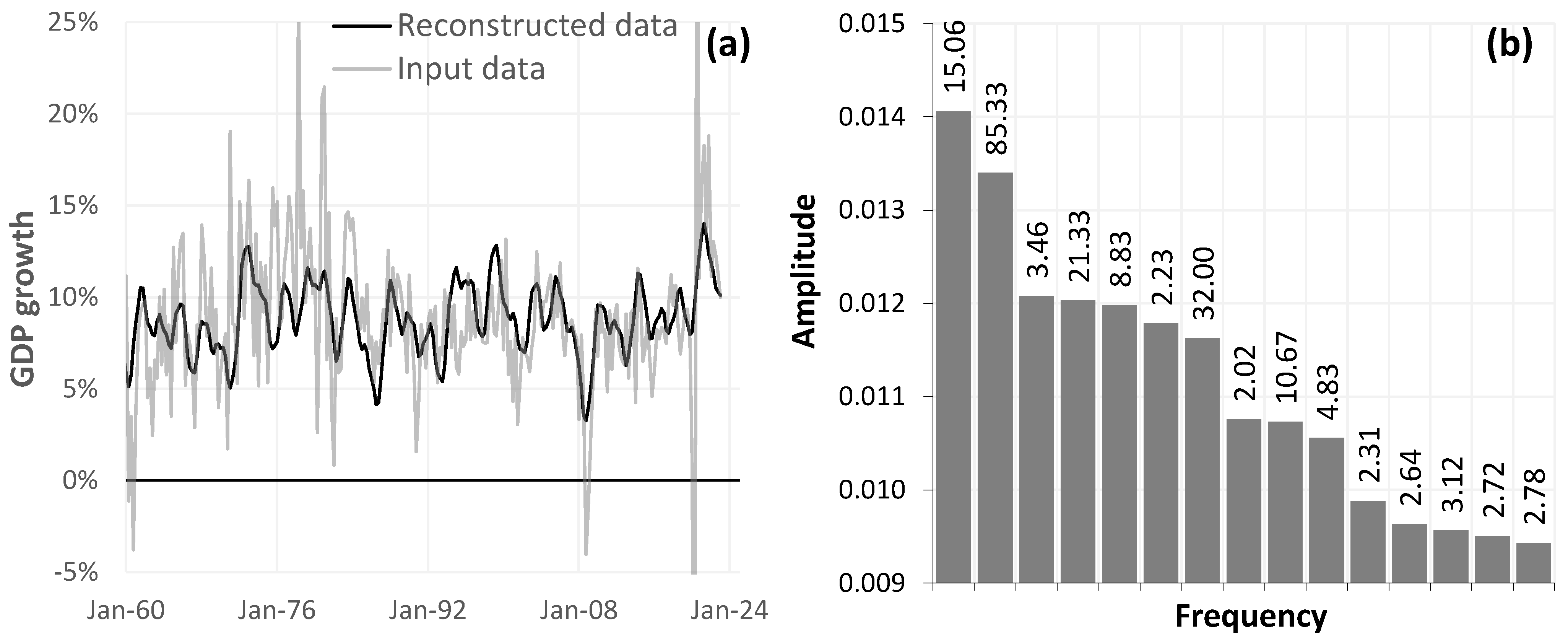
The Fast Fourier transform assumes that the input signal is stationary; however, nominal GDP data are not stationary. The implication thereof is that this is not an accurate representation of the time series, and Fourier analysis would identify spurious cycles stemming from the non-stationary data series. The quarter-on-quarter percentage differences were thus calculated to produce the return series and convert the data to be stationary. Figure 1a,b depict the Fourier analysis output. These returns contain a non-trending mean and they do not scale with time, meaning they are sufficient for use in the Fourier analysis framework.

There is a plethora of different factors that drive business cycles, including total factor productivity, shocks to terms of trade, fiscal and monetary policy shocks, oil price shocks, and many others. These driving forces are influenced by various domestic and external factors, e.g., the US business cycle is driven by national factors underpinned by a combination of productivity shocks and fiscal factors (Crucini et al. 2011). The business cycle exists as a complex interplay amongst numerous components, and this creates a noisy signal. This is illustrated by the input data in Figure 1a, whilst the reconstructed data represent the Fourier analysis output. Fourier analysis converts the time series of quarterly GDP returns from a time-domain representation into a frequency-domain representation. The time series is decomposed into a series of sine and cosine waves that exactly mimic the behaviour of the original series. The reconstructed data in Figure 1a show the resultant Fourier-transformed series with noise (frequencies with low amplitudes) removed. Two dominant frequencies are evident: a 15.06 quarter cycle and an 85.33 quarter cycle, shown in Figure 1b.1 These frequencies are expressed in quarterly terms, which translate to 3.76 and 21.33 years, respectively.

The characteristics of the business cycles of the US are announced by the National Bureau of Economic Research (NBER), and these data are often used as a benchmark in academic literature (Everts 2006). The NBER affirms the minimum and maximum durations to be 6 and 43 quarters, with an associated mean of 24.86 quarters. The dominant frequency assigned by this analysis falls within the envelope. On the other hand, the second-most prominent frequency exists beyond NBER’s upper and lower benchmarks. The magnitude of factors that contribute to the US business cycle produces a very noisy signal (Figure 1a), and the implication thereof is that many of the frequencies depicted in Figure 1b are spurious and irrelevant. The frequency of 85.33 may be a noisy signal, but it should be noted that this stems from an extensive dataset that comprises 256 quarters and it exhibits a significant amplitude. This frequency also exhibits properties consistent with long wave cycles that are generally driven by technological advancements and major innovations (Kondratieff 1926).

3.2. Energy

• Oil Price Cycles

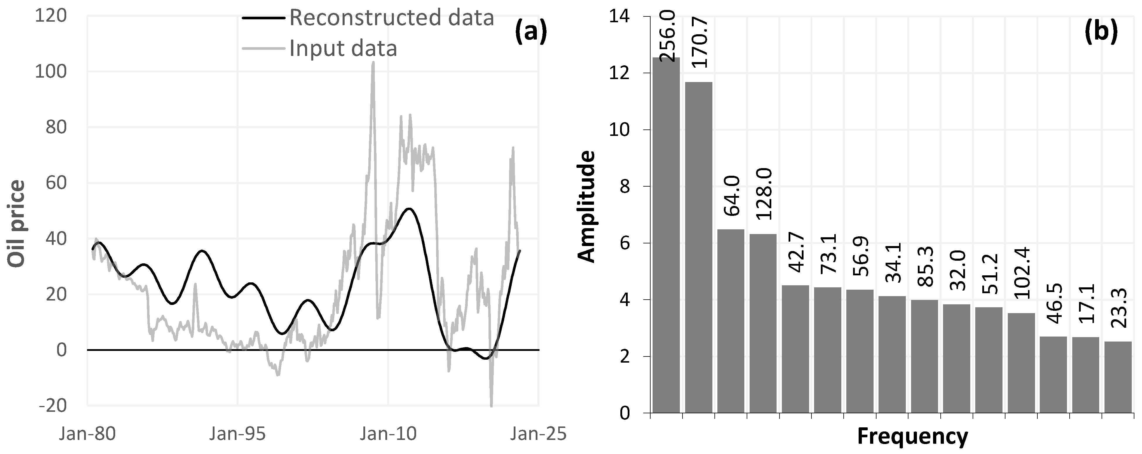
Erdem and Ünalmış (2016) identify three super-cycles in oil prices (1861–1882, 1966–1996, 1996–ongoing) and further suggest that business cycles in the US economy follow oil prices before the 1990s. These findings supplement Hamilton’s (1983) argument that post-war US recessions are largely caused by oil price hikes. Kyo and Noda (2017) also affirm that peaks in real oil prices lead to turning points in the Japanese business cycle, and this connection is noted to become stronger after the 2000s. Oil prices are known to be procyclical, a fact borne out by the correlation of oil price fluctuations and industrial production, observed since the turn of the century. Figure 2a,b illustrate the FFT of crude oil prices and Figure 3 the signal’s associated frequencies.

Figure 2a,b reveal two dominant frequencies of 256 and 170.7 months. The power or amplitude of each frequency component (which denotes the importance of the specific frequency in determining the original signal) is plotted against its period in Figure 3.

The periodogram in Figure 3 further exemplifies the dominance of the 256.0- and 170.7-month signals, which boast significant amplitudes relative to other frequencies. There are 512 data points in all the commodity price datasets, and the prominent cycle at 256 months is likely to be a harmonic of these inputs. In the context of Fourier analysis, a harmonic refers to a component of a complex signal or waveform that has a frequency that is an integer multiple of the fundamental frequency. The fundamental frequency represents the lowest frequency component of a periodic signal, and harmonics are subsequent integer multiples of this fundamental frequency. For example, if the fundamental frequency were $f$, the harmonics would be $2f$, $3f$, $4f$, and so on. The dominant frequency at 170.7 months (14.2 years) appears to be evidence of a consistent medium-run cycle in crude oil prices.

This result falls within the category of medium-run cycles that are defined as movements with periods of 8–20 years (Cuddington and Jerrett 2008; Erdem and Ünalmış 2016). This frequency is approximately four times the dominant frequency found within the US business cycle. These findings provide evidence of a relationship between crude oil price cycles and the US business cycle. Oil is closely tied to economic activity and industrial demand and may be procyclical. This relationship is exacerbated by factors such as increased industrial production, construction activities, and consumer spending. The factors that underpin this relationship also exist within Erten and Ocampo’s (2013) framework, which serves to provide insight into the long-term behaviour of commodity prices. Furthermore, these results bear notable similarities to those of Kyo and Noda (2017) and Erdem and Ünalmış (2016). The development of horizontal drilling and hydraulic fracking during the shale gas revolution reinvigorated the crude oil industry in the US, so much so that the country was a net energy exporter in 2019 and the world’s largest oil producer for the first time since 1952. This development is accompanied by upswings in the crude oil price cycle (Figure 2a) and the US business cycle (Figure 1a). The dominant frequency of the US business cycle is approximately half that of the crude oil cycle, which may be indicative of the emergence of a notable trend. Serletis and Shahmoradi (2005) found that crude oil prices are a useful guide for US monetary policy and these results reveal further evidence of a relationship between the two.

• Natural Gas

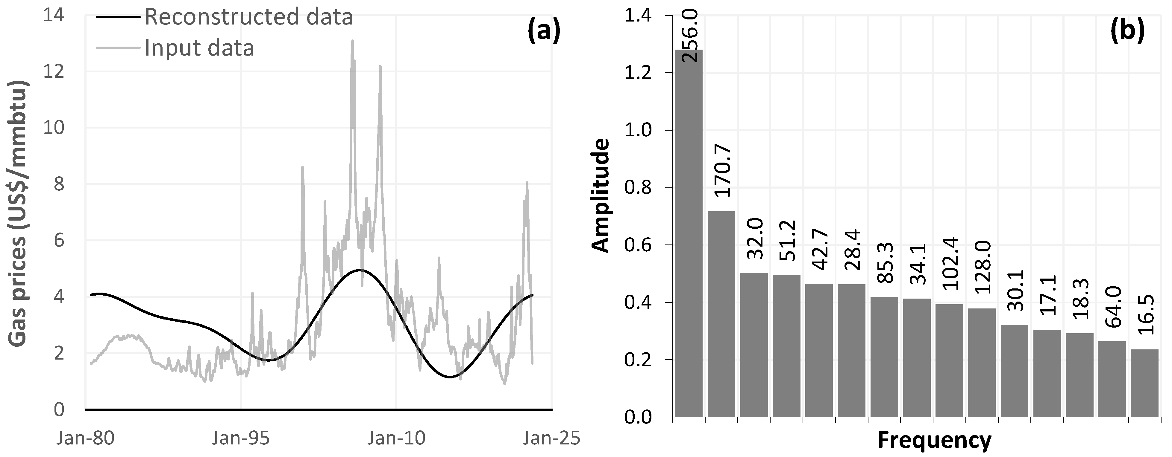
The chemical makeup of natural gas has implications for its use and application, for example, the presence of certain hydrocarbon gases in natural gas can affect its energy content, heating value and suitability for different purposes, including power generation and industrial processes (IEA 2023). Figure 4a,b show the price cycles of US natural gas.

Reconstructed data show a much longer wave in comparison to the crude oil price cycle, particularly from 1996 onwards (Figure 2a and Figure 4a). The North American energy industry underwent significant structural changes that had a significant impact on the environment in which producers, industrial customers, and transmission companies operate. The North American Free Trade Agreement signed in 1993 by the US, Canada, and Mexico focused on deregulation and increasing the efficiency in the energy industry. This was supplemented the Natural Gas Decontrol Act of 1989 in the United States (Serletis and Shahmoradi 2005).

The US natural gas price cycle has two dominant frequencies of 256.0 and 170.7 months: these are shown in Figure 4 and Figure 5. The presence of the 170.7-month frequency is a common feature between these oil and gas price cycles, reinforcing the possibility of a shared trend between these price cycles and the US business cycle. Caution should be exercised when making any concrete claims pertaining to 256.0-month cycles throughout the commodity price dataset owing to the possibility of it being a harmonic. However, the 256.0-month cycle is more dominant in this example and the plausibility of this frequency is bolstered by the shape of the reconstructed data in Figure 4a. The timeframe from trough to trough after 1996 is approximately 18 years and this period exists within the upper region of medium-run cycles (Schumpeter 1939).

The US natural gas industry has experienced extensive structural changes and technological advancements since the 1990s. The emergence of horizontal drilling and hydraulic fracking have allowed access to previously uneconomical shale gas reservoirs. Shale gas production is one of the most transformative changes in the US natural gas industry and it has resulted in a surge in domestic natural gas production, which in turn has led to the US becoming a net exporter of natural gas (Baffes and Kabundi 2021). The shale gas revolution is perpetuated by the development of liquefied natural gas infrastructure and an ongoing pipeline network expansion. These in tandem with market liberalisation outline a telling example of how structural changes and technological advances impact the US natural gas price cycle. These factors have increased the price ceiling and ultimately may be stimulating the development of longer-wave cycles in this market. Serletis and Shahmoradi’s (2005) findings state that natural gas is procyclical and lags the cycle of industrial production. In addition, natural gas prices are held to be positively contemporaneously correlated with US consumer prices and lead the cycle of consumer prices, highlighting the potential for natural gas prices to be a useful guide for US monetary policy. These findings implicate a distinct relationship between the US business cycle and US natural gas prices. Evidence of a pre-existing relationship provides a basis for the claim that the structural changes and technological innovation may be stimulating longer cycles in the US natural gas commodity price cycle.

3.3. Agriculture

• Maize, Wheat and Rice

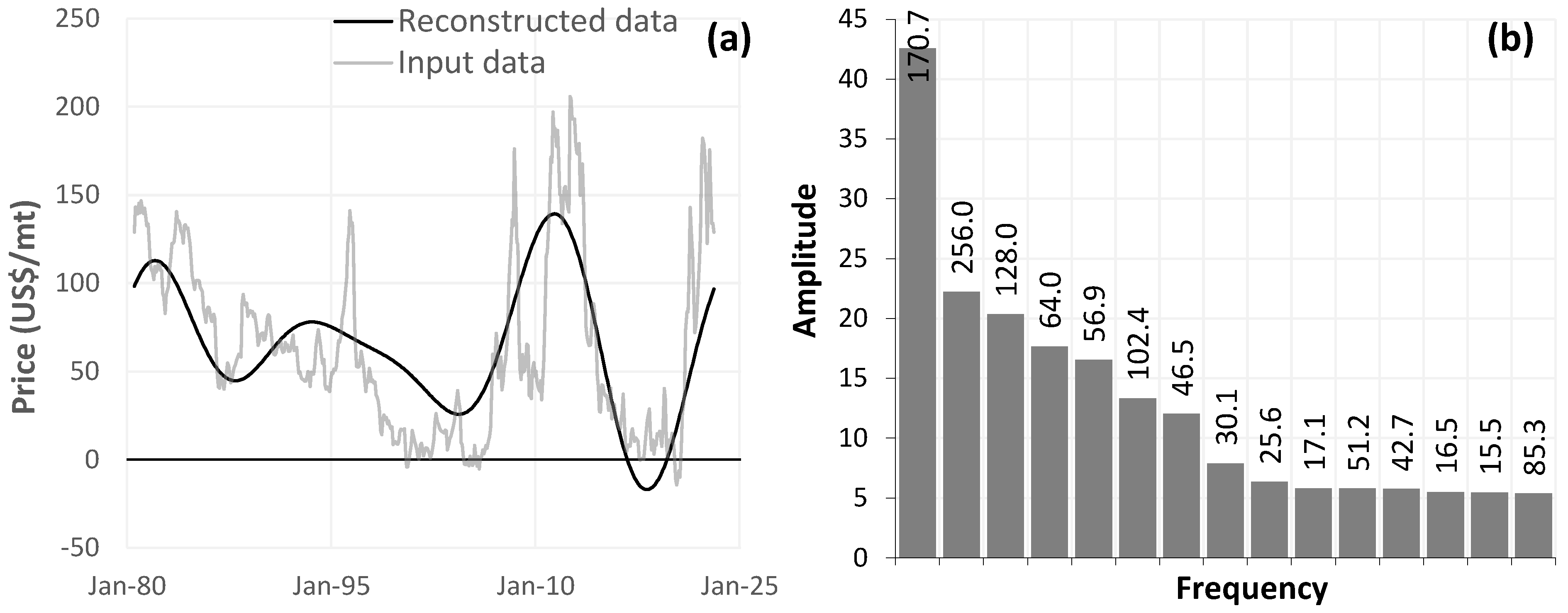
The agricultural sample comprises a cool season (wheat), warm season (maize) and staple (rice) crop. Each of these commodities has unique climate requirements, wherein each crop thrives in a different set of conditions (Sharma et al. 2022). This composition of crops also accounts for a substantial amount of the world’s arable land. Agricultural cycles are stimulated by weather conditions, supply–demand imbalances, government policy and market speculation. In addition, these commodities exhibit a co-movement with energy prices, whilst sharing a negative relationship with real income (consistent with the Prebisch-Singer hypothesis) (Baffes and Haniotis 2016. Figure 6a shows the Fourier analysis of maize prices during the sample period. The maize price cycle does not display a particularly noisy signal, having only one dominant frequency of 170.7 months, captured in Figure 6b.)

The reconstructed data show one of the more consistent cycles in this study. The food–energy nexus is subject to great attention from policymakers, and crude oil markets are maintained to play a significant role in explaining fluctuations in prices and the associated volatility of agricultural commodities (Vo et al. 2019). Wheat and maize have dominated the food security debate, with maize prices being deemed to be more sensitive to changes in stock (Baffes and Haniotis 2016. These factors are accompanied by different environmental conditions, all of which combine to create the maize price cycle.)

Figure 6b shows the maize price cycle to have one dominant frequency of 170.7 months (roughly 14 years), whilst the frequencies of 256, 128 and 64 are all likely harmonics. The associated amplitude for the dominant frequency is 42.56—a higher amplitude is indicative of a frequency with a greater intensity, meaning the components with lower amplitudes are discarded as ‘noise’. The Fast Fourier transform generates a prominent signal (Figure 7) that has also appeared within the crude oil and US natural gas price cycles.

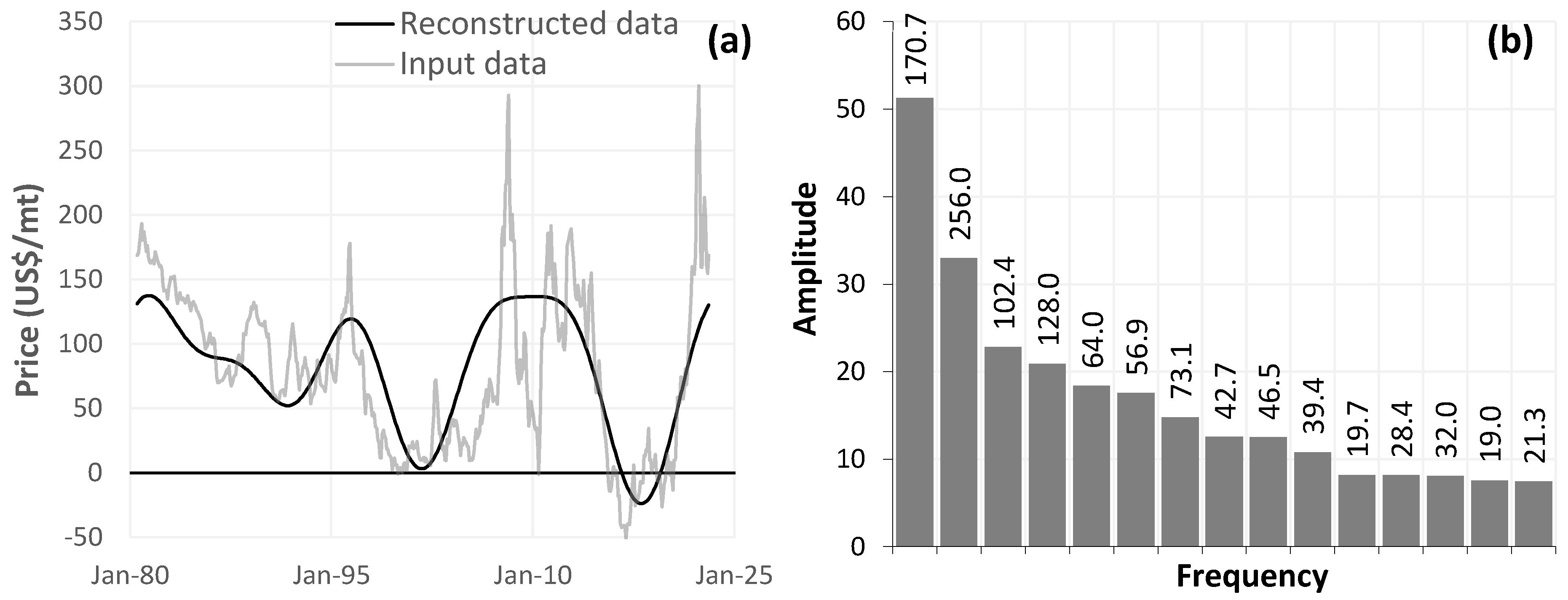
Figure 8 shows the Fourier analysis of the wheat price cycle.

The reconstructed wheat cycle details a growingly uniform pattern, and this is further evidence of the strength and consistency of the 170.7-month frequency because agricultural price cycles are subject to a variety of different factors, including different weather conditions. The persistence of the same dominant frequency between cool season and warm season crops is noteworthy. In addition, the periodogram in Figure 9 illustrates the substantial amplitude differentials and thus provides further evidence of the prominence of this cycle.

The dominant frequency is associated with a high amplitude, as seen in Figure 9. In addition, the periodogram above illustrates the substantial amplitude differentials and thus provides further evidence of the prominence of this cycle.

Agricultural commodities are not usually defined as procyclical, but rather exist as commodities that are subject to the influence of various factors that may have cyclical patterns, such as crude oil price cycles (Hong Vo et al. 2019). However, it is possible that there may be a relationship between the dominant 14.23- and the 3.76-year frequencies of the agricultural commodities and the US business cycle, discussed in the following section.

• El Niño–Southern Oscillation (ENSO)

The El Niño–Southern Oscillation (ENSO) is a climate phenomenon that refers to the coupled interaction between the ocean and the atmosphere in the tropical Pacific region. It is characterised by the alternating phases of El Niño and La Niña, which represent opposite extremes of the ENSO cycle. ENSO affects the supply, and to some extent the demand of primary commodities, whilst there is a statistical linkage between sea surface temperature anomalies and agricultural commodity prices that manifests a sound price forecasting for commodities produced in the tropics. El Niño and La Niña events occur irregularly and can last anywhere between six months and two years (Ubilava 2017). These events exist as a natural shock that influences rainfall and weather patterns in numerous different countries, including the US.

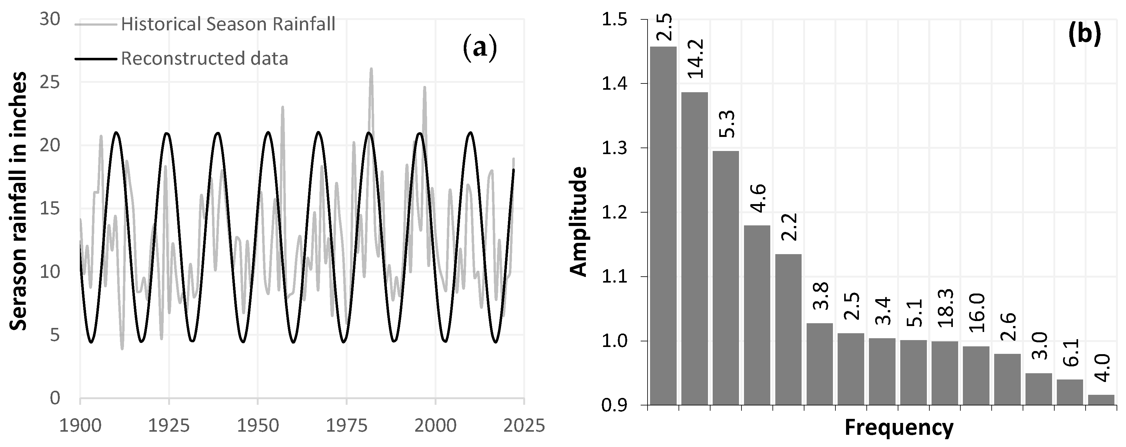
Fourier analysis was conducted on historical rainfall in the US as a means of filtering out some of the random noise associated with rainfall patterns in a bid to investigate one of the fundamental factors that contributes to the development of agricultural price cycles. Figure 10a,b shows the results obtained.

Rainfall patterns are subject to their own driving factors and unique shocks such as El Niño or El Niña. Therefore, the Fourier analysis performed above successfully removes the random noise and highlights the dominant underlying frequencies. This result displays the most consistent cycle in the research, with a 14.2-year cycle (from trough to trough).

Historical rainfall data are annual, and the dominant frequencies are 2.5, 14.2 and 5.3 years. The most compelling frequency is that of 14.2 years and this represents the full cycle, as seen in Figure 10a. This cycle closely matches the dominant agricultural cycle of 14.2 years, and this alignment outlines a potential link between rainfall patterns and agricultural productivity, which can impact crop yields and subsequently influence commodity prices. In addition, the US business cycle exhibits a dominant frequency that is approximately one quarter the length of the agricultural commodity price and historical rainfall cycles.

This finding suggests that it is possible that some interconnection exists between the broader economic conditions reflected in the business cycle and the agricultural sector. Changes in economic activity, consumer spending, and overall market conditions could influence the demand for agricultural commodities, subsequently impacting their prices. The synchronisation of the cycles in commodity prices, the business cycle, and rainfall patterns suggests that agricultural markets are interconnected with broader economic factors and climatic conditions. Economic factors, such as changes in global demand, trade policies, and financial market fluctuations, could influence commodity prices and align with the broader business cycle. Weather patterns, particularly rainfall, can significantly affect agricultural productivity and subsequently impact commodity prices. The alignment of the agricultural cycle with the historical rainfall cycle indicates a potential relationship between the two. Ubilava’s (2017) findings suggest that agricultural commodities display a robust response to ENSO shocks and outlines the forecast potential associated with this climate phenomenon. These results bear some notable similarities through the identification of some alignment patterns amongst US historical rainfall, the US business cycle, and the agricultural commodity price cycles in this research. These findings seem to bolster the plausibility of climate phenomena displaying forecasting potential.

3.4. Metals

• Precious Metals

Metals have different practical functions that serve to cultivate a variety of responses to changing market conditions. The analysis was conducted on three precious metals (gold, silver, and platinum) and three base metals (copper, aluminium, and nickel). The principal function of precious metals is in the storing of economic value: in times of prevailing crisis, gold, amongst other precious metals, is considered a reliable hedge in terms of portfolio diversification (Umar et al. 2021). Figure 11 shows the Fourier analysis of gold prices during the sample period.

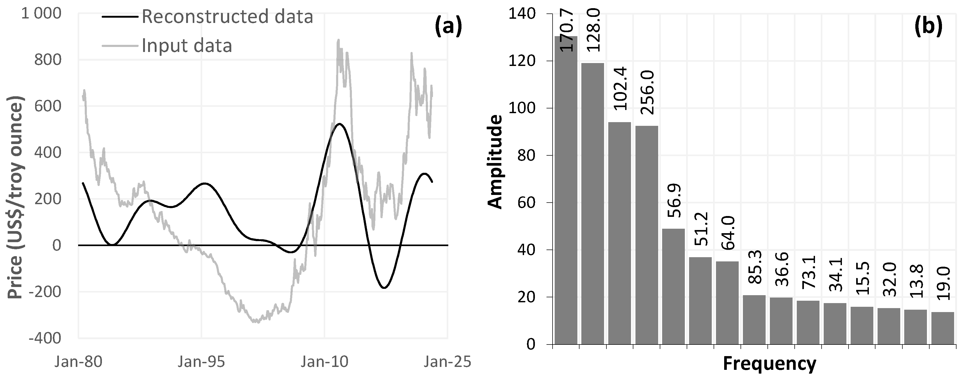
Figure 11a shows the positive response exhibited by gold prices during the COVID-19 pandemic, which is in line with the safe-haven2 properties of gold, particularly during recessionary times (Bakas and Triantafyllou 2020). These safe-haven properties coupled with the storing of economic value have rendered gold, amongst other precious metals, to be described as countercyclical. Gold and silver are examples of metals that are countercyclical, as their prices rise during times of economic uncertainty, as seen above in Figure 11a (price rise during the 2008 global financial crises and upon the inception of the COVID-19 pandemic in 2020). Results indicate two dominant frequencies of 170.7 months and 128.0 months. This is yet another example of a prominent 170.7-month medium-run cycle, meaning this frequency is a consistent feature across all the different commodity groups in this research.

This trend is shared amongst procyclical (crude oil, natural gas) and countercyclical commodities (gold and silver). The prevalence of this frequency is peculiar. The periodogram in Figure 12 illustrates the comparative intensity of the dominant 170.7-month frequency.

The gold reconstructed data and the US business cycle reconstructed data share an inverse relationship. Figure 1a and Figure 11a do not share uniform timelines; however, see years 1984 and 2023 and the corresponding reconstructed data values in these figures. The gold reconstructed data have a trough in 1984, whilst the US business cycle reconstructed data experience a peak at that time. The opposite is true in 2023, with gold prices reaching a peak and the US business cycle descending towards a trough (Figure 1a and Figure 11a). This provides evidence of the countercyclical relationship shared between gold and the US business cycle, which agrees with the findings of Bredin et al. (2015).

The approximate relationship between the dominant frequencies (one quarter of the gold price cycle aligning with the US business cycle) suggests a potential lagged relationship or interplay between the two. It implies that the US business cycle may experience economic fluctuations and changes in investor sentiment that respond to or follow movements in the gold market. This could be due to changes in financial markets, investor behaviour, and the impact of gold prices on economic confidence.

Gold and silver are often thought of as substitutes; however, Batten et al. (2010) suggests that broader structural issues and differences between these commodities may mean they do not represent one monolithic asset class. Kucher and McCoskey (2017) affirm there to be cointegrating relationships between weekly prices of gold and silver; however, the long-run relationships are deemed to be unstable, indicating a separation of precious metal prices during certain periods of time, such financial crises, and economic contractions. Figure 13 and Figure 14 detail the Fourier analysis of silver prices.

Fourier analysis of silver prices showed a dominant frequency of 170.7 months with an amplitude of 3.0. The second- and third-most dominant frequencies were 128.0 and 256.0 months, which are both likely to be harmonics. Silver and gold share almost identical reconstructed data as well as a common dominant frequency of 170.7 months. Silver displays the same countercyclical properties as gold during the sample period. The inference thereof is that the approximate relationship between the dominant frequencies (one quarter of the silver price cycle aligning with the US business cycle) suggest the same possible lagged relationship between silver and the US business cycle as seen in the analysis of gold prices above.

• Base Metals

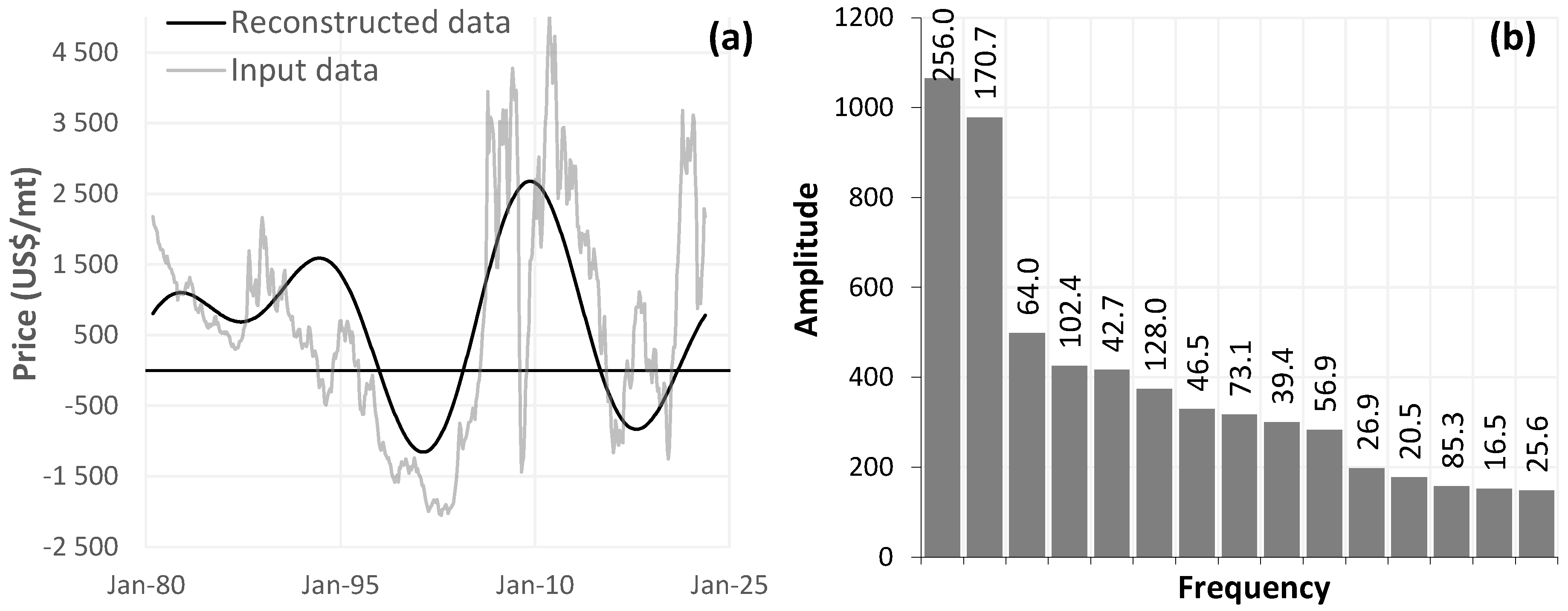
This research analyses copper, aluminium, and nickel price cycles, all of which are base metals. Base metals are cheaper and more readily extractible than their precious counterparts, and are often used in various industrial and manufacturing capacities. Copper is an excellent conductor of electricity, rendering it paramount for electrical wiring and power transmission. The extensive use of copper means that it is often used as a barometer for the overall health of the global economy (van der Nest and van Vuuren 2023). The Fourier analysis of copper prices is shown in Figure 15.

The copper reconstructed data show the most prominent cycle in the commodity price dataset. Fourier analysis once again delivers two dominant 256.0-month and 170.7-month frequencies, with associated amplitudes of 1065 and 978. The frequency amplitude-relations are illustrated in Figure 15b and Figure 16.

There is potential for the 256.0-month cycle to be a harmonic, due to the 512-month data sample and this is supplemented by presence of two additional harmonic frequencies of 64.0 and 128.0 months as seen above. Cuddington and Jerrett (2008) document the presence of four super-cycles within copper price cycles, amongst five other metals.

The length of this dataset does not allow for a meaningful analysis of these long-wave cycles. However, it is plausible that the presence of this dominant 256.0-month cycle provides further evidence of a long-wave cycle in the copper price cycle.

The prevalence of the 170.7-month medium-run cycle reappears in the analysis of copper prices. Base metals display procyclical properties and Yin et al. (2020) affirm copper to exhibit procyclical behaviour. Copper’s procyclical trend means its prices tend to move in the same direction as the US business cycle. Copper’s price movements can reflect changes in industrial production, construction activity, and global economic conditions. A positive correlation between copper prices and the business cycle bolsters the plausibility of a relationship between observed dominant frequencies (14.23 and 3.76) of these entities.

4. Conclusions

This article explores the connections between the US business cycle and various commodity price cycles, revealing significant insights. A notable discovery is the consistent presence of a roughly 14-year (170.7-month) medium-term cycle within the commodity dataset, albeit with varying prominence across commodities. This cycle aligns with the US business cycle, which exhibits a dominant 3.76-year cycle—around a quarter of the 14-year commodity cycle. These relationships are influenced by diverse factors specific to each commodity, adding complexity to the understanding of commodity price dynamics. The phases of these cycles, influenced by factors like demand shifts and oversupply, have direct effects on output and employment.

The implications of these findings are crucial for comprehending agricultural commodity price dynamics and broader economic influences. Economic activities, consumer spending, and market conditions all impact the demand for agricultural commodities, consequently affecting prices. The study’s spotlight on the synchronisation between commodity price, business, and historical rainfall cycles underscores the interplay between economic and climatic factors in shaping agricultural markets. Global demand changes, trade policies, and financial market fluctuations align with the broader business cycle, while weather patterns, especially rainfall, significantly influence agricultural productivity and prices.

The shale gas revolution’s impact on the US crude oil and natural gas industries is highlighted, with these sectors exhibiting cycles tied to the US business cycle. The presence of a roughly 14-year frequency in both industries, accompanied by procyclical behaviour, indicates a potential lead or lag relationship between these commodities and the US business cycle. The study also reinforces the cointegration of silver and gold prices, implying potential substitution between these assets due to their countercyclical nature.

This research’s practical applications extend to risk management and hedging strategies. Understanding the timing and phases of the business cycle and medium-term commodity cycles can aid market participants in anticipating and managing price volatility. Aligning production and marketing strategies with expected commodity price movements mitigates risk and optimises profitability. Investors and policymakers alike can benefit from this knowledge, informing portfolio management, risk mitigation strategies, and economic growth promotion.

The study underscores the need to consider both economic and climatic factors in analysing commodity price dynamics. The intricate interplay between the US business cycle, commodity cycles, and historical rainfall patterns highlights the complexity of agricultural commodity pricing. Policymakers must formulate comprehensive strategies considering economic policies, market conditions, climate change, and weather patterns to ensure the agricultural sector’s resilience in changing conditions. However, the relationship’s complexity and susceptibility to external factors necessitate ongoing research and analysis for a refined understanding of these interactions.

• Limitations

FFT has revolutionised many fields, including signal processing and data analysis (Walker 1996). However, it has some noteworthy limitations. It requires a fixed number of samples, which limits the number of input data points to $2^n$, where $n\in \mathbb{Z}$ (Cooley and Turkey 1965). This assumption has dictated the composition of all the datasets in this research. For example, the commodity price dataset was limited to 512 monthly data points between July 1980 and February 2023. The combination of the FFT constraint and limited data availability underpin the selection of the sample set. Other techniques, such as wavelet analysis, can use any amount of data and detect any frequency. In addition, this research assumes cyclicality, i.e., history mimics the future. This introduces its own limitations, as FFT does not effectively pick up once-off events such as COVID-19. The pandemic was a unique transitory shock independent of weather or financial causes, but it had an undeniable impact on frequency analyses.

Previous research conducted on super-cycles in different commodity markets incorporates the use of the HP and BK filters. These filters were not used; however, it is unlikely that the use of these methods would have had a dramatic effect on the results, as they would produce periodograms with less noise, but dominant frequencies would persist. Employing FFT resulted in inconclusive claims regarding the detection of long wave cycles. There was some evidence of these within the US natural gas and aluminium price cycles; however, the use of wavelet analysis in tandem with these filters would be a more suitable approach in terms of extracting noteworthy results relating to these potential long wave cycles.

• Limitations and Recommendations for Further Research

Some limitations that have influenced this research include that FFT requires a fixed number of discrete samples, which limits the number of input data points to $2^n$, where $n\in \mathsf{{\rm Z}}$ (Cooley and Turkey 1965). For example, the commodity price dataset was limited to 512 monthly data points between July 1980 and February 2023. The combination of the FFT constraint and limited data availability underpin the selection of the sample set. Other techniques, such as wavelet analysis, can use any-sized data sample and detect any frequency. This research also assumes cyclicality, i.e., what happened in the past will mimic the future, which introduces its own limitations, as the FFT does not effectively identify once-off events such as COVID-19. The pandemic was a unique transitory shock that had nothing to do with weather or financial causes; however, it had an undeniable impact on frequency analyses.

Fourier analysis of price cycles for US natural gas and aluminium hints at the presence of extended cycles in these markets. However, Fourier transform might not be the most optimal approach for understanding longer cycles. A more promising avenue could involve wavelet analysis over a greater time span, which may yield more intriguing outcomes regarding potential long wave or super-cycles within these markets.

The findings indicate some level of interaction and synchronisation among rainfall patterns, the US economic cycle, and agricultural price cycles. It is worth considering that distinct weather phenomena could influence commodity prices across different geographical regions globally. For instance, analysing potential wildfire frequency trends in Northern Australia might offer valuable insights for farmers, policymakers, and other stakeholders seeking to make informed decisions.

References

1. Ahmed, Walid. 2022. On the higher-order moment interdependence of stock and commodity markets: A wavelet coherence analysis. The Quarterly Review of Economics and Finance 83: 135–51. [Google Scholar] [CrossRef]
2. Askey, Richard, and Deborah Tepper Haimo. 1996. Similarities between Fourier and Power Series. The American Mathematical Monthly 103: 297–304. [Google Scholar] [CrossRef]
3. Baffes, John, and Alain Kabundi. 2021. Commodity price shocks: Order within Chaos? Policy Research Working Papers, 1–75. [Google Scholar] [CrossRef]
4. Baffes, John, and Tassos Haniotis. 2016. What explains agricultural price movements? Journal of Agricultural Economics 3: 706–21. [Google Scholar] [CrossRef]
5. Bakas, Dimitrios, and Athanasios Triantafyllou. 2020. Commodity price volatility and the economic uncertainty of pandemics. SSRN Electronic Journal 193: 1–5. [Google Scholar] [CrossRef]
6. Batten, Jonathan, Cetin Ciner, and Brain M. Lucey. 2010. The macroeconomic determinants of volatility in precious metals markets. Resources Policy 35: 65–71. [Google Scholar] [CrossRef]
7. Baxter, Marianne, and Robert G. King. 1999. Measuring business cycles: Approximate band-pass filters for economic time series. The Review of Economics and Statistics 81: 575–93. [Google Scholar] [CrossRef]
8. Boehm, E. A., and P. M. Summers. 1999. Analysing and forecasting business cycles with the aid of economic indicators. International Journal of Management Reviews 1: 245–77. [Google Scholar] [CrossRef]
9. Bredin, Don, Thomas Conlon, and Valerio Potì. 2015. Does gold glitter in the long-run? Gold as a hedge and safe haven across time and investment horizon. International Review of Financial Analysis 41: 320–28. [Google Scholar] [CrossRef]
10. Brown, James Ward, and Ruel Vance Churchill. 1993. Fourier Series and Boundary Value Problems, 5th ed. New York: Mcgraw-Hill College. [Google Scholar]
11. Christiano, Lawrence, and Terry Fitzgerald. 2003. The band pass filter. International Economic Review 44: 435–65. [Google Scholar] [CrossRef]
12. Cooley, James W., and John W. Tukey. 1965. An algorithm for the machine calculation of complex Fourier series. Mathematics of Computation 19: 297–301. [Google Scholar] [CrossRef]
13. Crucini, Mario, M. Ayhan Kose, and Christopher Otrok. 2011. What are the driving forces of international business cycles? Review of Economic Dynamics 14: 156–75. [Google Scholar] [CrossRef]
14. Cuddington, John T., and Daniel Jerrett. 2008. Super cycles in real metals prices? IMF Staff Papers 55: 541–65. [Google Scholar] [CrossRef]
15. Erdem, Fatma Pınar, and İbrahim Ünalmış. 2016. Revisiting super-cycles in commodity prices. Central Bank Review 16: 137–42. [Google Scholar] [CrossRef]
16. Erten, Bilge, and José Antonio Ocampo. 2013. Super cycles of commodity prices since the mid- nineteenth century. World Development 44: 1–34. [Google Scholar] [CrossRef]
17. Everts, Martin P. 2006. Duration of business cycles. SSRN Electronic Journal, 1–30. [Google Scholar] [CrossRef]
18. Fernández, Andrés, Stephanie Schmitt-Grohé, and Martín Uribe. 2020. Does the commodity Super Cycle matter? NBER Working Paper, 1–32. [Google Scholar] [CrossRef]
19. Focacci, Antonio. 2023. A Wavelet investigation of periodic long swings in the economy: The original data of Kondratieff and some important series of GDP per capita. Economies 11: 231. [Google Scholar] [CrossRef]
20. Gubler, Matthias, and Matthias S. Hertweck. 2013. Commodity price shocks and the business cycle: Structural evidence from the US. Journal of International Money and Finance 37: 324–52. [Google Scholar] [CrossRef]
21. Hamilton, James D. 1983. Oil and the macroeconomy since World War II. Journal of Political Economy 91: 228–48. [Google Scholar] [CrossRef]
22. Heap, Alan. 2005. China—The Engine of Commodities Super Cycle. New York: Citigroup Smith Barney. [Google Scholar]
23. IEA. 2023. International Energy Agency. IEA. Available online: https://www.iea.org/ (accessed on 3 May 2023).
24. Jacks, David S. 2019. From boom to bust: A typology of real commodity prices in the long run. Cliometrica 13: 201–20. [Google Scholar] [CrossRef]
25. Jacks, David S., and Martin Stuermer. 2020. What drives commodity price booms and busts? Energy Economics 85: 1–8. [Google Scholar] [CrossRef]
26. Jerrett, Daniel, and John T. Cuddington. 2008. Broadening the statistical search for metal price super cycles to steel and related metals. Resources Policy 33: 188–95. [Google Scholar] [CrossRef]
27. Kondratieff, Nikolai. 1926. The Long Wave Cycle. New York: Richardson & Snyder. [Google Scholar]
28. Krantz, S. G. 1999. How to Teach Mathematics. New York: American Mathematical Soc. [Google Scholar]
29. Kucher, Oleg, and Suzanne McCoskey. 2017. The long-run relationship between precious metal prices and the business cycle. The Quarterly Review of Economics and Finance 65: 263–75. [Google Scholar] [CrossRef]
30. Kyo, Koki, and Hideo Noda. 2017. Correspondence between turning points in trend of oil price and business cycles in Japan. Advances in Engineering Research 94: 388–93. [Google Scholar] [CrossRef]
31. Liu, L., E. Paki, J. Stonehouse, and J. You. 2012. Cycle Identification: An Old Approach to (Relatively) New Statistics. Development, Environment, Satellites, and Strategy, Statistics. Paper presented at the 53rd New Zealand Association of Economists Conference, Palmerston North, New Zealand, June 27; pp. 1–21. [Google Scholar]
32. Masset, Philippe. 2008. Analysis of financial time-series using Fourier and wavelet methods. SSRN Electronic Journal, 1–36. [Google Scholar] [CrossRef]
33. Modesto Irrigation District. 2023. Historical Season Rainfall. Weather Data. Available online: https://www.mid.org/weather/historical.jsp. (accessed on 5 June 2023).
34. Omekara, Chukwuemeka O., Emmanuel J. Ekpenyong, and Michael P. Ekerete. 2013. Modelling the Nigerian inflation rates using periodogram and Fourier Series Analysis. CBN Journal of Applied Statistics 4: 51–68. [Google Scholar]
35. Phochanachan, Panisara, Nootchanat Pirabun, Supanika Leurcharusmee, and Woraphon Yamaka. 2022. Do bitcoin and traditional financial assets act as an inflation hedge during stable and turbulent markets? Evidence from high cryptocurrency adoption countries. Axioms 7: 339. [Google Scholar] [CrossRef]
36. Schumpeter, J. 1939. Business Cycles. New York: McGraw Hill, vols. 1 and 2. [Google Scholar]
37. Serletis, Apostolos, and Asghar Shahmoradi. 2005. Business cycles and natural gas prices. OPEC Review 1: 75–84. [Google Scholar] [CrossRef]
38. Sharma, Ramandeep Kumar, Sunny Kumar, Kamal Vatta, Raju Bheemanahalli, Jagmandeep Dhillon, and Krishna N. Reddy. 2022. Impact of recent climate change on corn, rice, and wheat in Southeastern USA. Scientific Reports 12: 16928. [Google Scholar] [CrossRef]
39. Stádník, Bohumil, Jurgita Raudeliūnienė, and Vida Davidavičienė. 2016. Fourier analysis for stock price forecasting: Assumption and evidence. Journal of Business Economics and Management 17: 365–80. [Google Scholar] [CrossRef]
40. Thomson, Daniel, and Gary van Vuuren. 2016. Forecasting the South African business cycle using Fourier analysis. International Business & Economics Research Journal 15: 175–92. [Google Scholar] [CrossRef]
41. Ubilava, David. 2017. The role of El Niño Southern oscillation in commodity price movement and predictability. American Journal of Agricultural Economics 1: 239–63. [Google Scholar] [CrossRef]
42. Umar, Zaghum, Mariya Gubareva, and Tamara Teplova. 2021. The impact of Covid-19 on commodity markets volatility: Analyzing time-frequency relations between commodity prices and coronavirus panic level. Resources Policy 73: 102164. [Google Scholar] [CrossRef] [PubMed]
43. van der Nest, Matthew, and Gary van Vuuren. 2023. Metal price behaviour during recent crises: Covid-19 and the Russia–Ukraine conflict. Journal of Economic and Financial Sciences 16: 819. [Google Scholar] [CrossRef]
44. Vo, Duc Hong, Tan Ngoc Vu, Anh The Vo, and Michael McAleer. 2019. Modelling the relationship between crude oil and agricultural commodity prices. Energies 7: 1344. [Google Scholar] [CrossRef]
45. Walker, Jams S. 1996. Fast Fourier Transforms. Boca Raton: CRC Press, vol. 24. [Google Scholar]
46. World Bank. 2021. Causes and Consequences of Metal Price Shocks. Available online: https://thedocs.worldbank.org/en/doc (accessed on 14 March 2023).
47. World Bank. 2023. Commodity Markets. Washington, DC: World Bank. Available online: https://www.worldbank.org/en/research/commodity-markets (accessed on 14 March 2023).
48. Yin, Libo, Jing Nie, and Liyan Han. 2020. Intermediary asset pricing in commodity futures returns. Journal of Futures Markets 11: 1711–30. [Google Scholar] [CrossRef]
Figure 1. (a) Fourier analysis and (b) frequency output of US GDP between Q2 1959 and Q1 2023. Source: authors’ calculations.
Jrfm 16 00462 g001
Figure 2. (a) Fourier analysis and (b) frequency output of crude oil prices between July 1980 and February 2023. Source: authors’ calculations.
Jrfm 16 00462 g002
Figure 3. Periodogram of crude oil price prices. Source: authors’ calculations.
Jrfm 16 00462 g003
Figure 4. (a) Fourier analysis and (b) frequency output of natural gas prices between July 1980 and February 2023. Source: authors’ calculations.
Jrfm 16 00462 g004
Figure 5. Periodogram of US natural gas prices. Source: authors’ calculations.
Jrfm 16 00462 g005
Figure 6. (a) Fourier analysis and (b) frequency output of maize prices between July 1980 and February 2023. Source: authors’ calculations.
Jrfm 16 00462 g006
Figure 7. Periodogram of maize prices. Source: authors’ calculations.
Jrfm 16 00462 g007
Figure 8. (a) Fourier analysis and (b) frequency output of wheat prices between July 1980 and February 2023. Source: authors’ calculations.
Jrfm 16 00462 g008
Figure 9. Periodogram of wheat prices. Source: authors’ calculations.
Jrfm 16 00462 g009
Figure 10. (a) Fourier analysis and (b) frequency output of historical rainfall in the US. Source: authors’ calculations.
Jrfm 16 00462 g010
Figure 11. (a) Fourier analysis and (b) frequency output of gold prices between July 1980 and February 2023. Source: authors’ calculations.
Jrfm 16 00462 g011
Figure 12. Periodogram of gold prices. Source: authors’ calculations.
Jrfm 16 00462 g012
Figure 13. (a) Fourier analysis and (b) frequency output of silver prices between July 1980 and February 2023. Source: authors’ calculations.
Jrfm 16 00462 g013
Figure 14. Periodogram of silver prices. Source: authors’ calculations.
Jrfm 16 00462 g014
Figure 15. (a) Fourier analysis and (b) frequency output of copper prices between July 1980 and February 2023. Source: authors’ calculations.
Jrfm 16 00462 g015
Figure 16. Periodogram of copper prices. Source: authors’ calculations.
Jrfm 16 00462 g016