Article

A Fourier Interpolation Method for Numerical Solution of FBSDEs: Global Convergence, Stability, and Higher Order Discretizations †

Department of Mathematics and Statistics, Concordia University, 1455 Boulevard de Maisonneuve Ouest, Montréal, QC H3G 1M8, Canada
*
Author to whom correspondence should be addressed.
A previous version of this paper was titled “Global convergence and stability of a convolution method for numerical solution of BSDEs” arXiv:1410.8595v1.
J. Risk Financial Manag. 2022, 15(9), 388; https://doi.org/10.3390/jrfm15090388
Submission received: 20 May 2022 / Revised: 26 August 2022 / Accepted: 30 August 2022 / Published: 31 August 2022
(This article belongs to the Special Issue Risk Management and Forecasting Methods in Finance)

Abstract

:
The convolution method for the numerical solution of forward-backward stochastic differential equations (FBSDEs) was originally formulated using Euler time discretizations and a uniform space grid. In this paper, we utilize a tree-like spatial discretization that approximates the BSDE on the tree, so that no spatial interpolation procedure is necessary. In addition to suppressing extrapolation error, leading to a globally convergent numerical solution for the FBSDE, we provide explicit convergence rates. On this alternative grid the conditional expectations involved in the time discretization of the BSDE are computed using Fourier analysis and the fast Fourier transform (FFT) algorithm. The method is then extended to higher-order time discretizations of FBSDEs. Numerical results demonstrating convergence are presented using a commodity price model, incorporating seasonality, and forward prices.
Mathematics Subject Classification (2000):
Primary: 60H10, 65C30; Secondary: 60H30

1. Introduction

A variety of numerical methods for backward stochastic differential equations (BSDEs) and forward-backward stochastic differential equations (FBSDEs) have been developed recently. Different applications call for innovative techniques for the efficient resolution of these systems. In finance and economics BSDEs are used for option pricing and hedging El Karoui et al. (1997), reflected BSDEs are used for modeling American options El Karoui et al. (1997), and quadratic BSDEs play an important role in continuous-time recursive utility Duffie and Epstein (1992) and other utility maximization problems.
Following the establishment of the well-posedness of BSDEs by Pardoux and Peng (1992) the first numerical procedures to emerge were partial differential equation (PDE) based methods such as the finite difference approach of Douglas et al. (1996). The PDE method is mainly devoted to coupled problems as is the spectral method of Ma et al. (2008). More recent numerical methods based on machine learning (Beck et al. 2019; Han and Long 2020; E et al. 2017, 2019, 2022) have been applied to the numerical solution of BSDEs which, given the connections between the theory of PDEs and their representations as BSDEs, in turn provides solutions to high dimensional PDEs. Spatial discretization methods were initiated by Chevance (1997) with a quantization approach to conditional expectations. However, it is only since Zhang (2004) and Bouchard and Touzi (2004) that a sound time discretization of (decoupled) FBSDEs is available. The quantization approach was then used in the multidimensional framework of Bally and Pages (2003); Bally et al. (2005) and the coupled FBSDE case of Delarue and Menozzi (2006). The theoretical basis for a multinomial approach for BSDEs was introduced by Briand et al. (2001) and Ma et al. (2002) and followed in practice by Peng and Xu (2011). Monte Carlo methods are the most prolific approach for numerical solutions of (F)BSDEs. They include the backward scheme of Zhang (2004), the Malliavin approach of Bouchard and Touzi (2004) and Crisan et al. (2010), the least-square regression approach of Gobet et al. (2005) and the iterative schemes Bender and Denk (2007) and Bender and Zhang (2008).
Additional approaches to numerical solution of BSDEs include the cubature method Crisan and Manolarakis (2012, 2014), Fourier-cosine expansions Huijskens et al. (2016); Ruijter and Oosterlee (2015, 2016), and the convolution method Hyndman and Oyono Ngou (2017). In introducing the convolution method, Hyndman and Oyono Ngou (2017) developed a local discretization error which includes an extrapolation error. The extrapolation error component is exclusively produced by the fast Fourier transform (FFT) algorithm and the underlying trigonometric interpolation used to compute conditional expectations. To improve the performance of the convolution method it is desirable to eliminate the extrapolation error, and improve the error bound, with an alternative implementation of the FFT algorithm.
In this paper, we propose an alternative space grid for the convolution method, instead of the rectangular grid in Hyndman and Oyono Ngou (2017), which eliminates the extrapolation error, leads to a globally convergent numerical solution for the (F)BSDE, and provides explicit convergence rates. We also apply the numerical method to the Runge–Kutta schemes for FBSDEs proposed by Chassagneux and Crisan (2014). The tree-like nature of the alternative grid avoids extrapolations and leads to a global error bound for the BSDE approximate solutions. Further, the implementation of the convolution method originally presented in Hyndman and Oyono Ngou (2017) is simplified by using an alternative parametric transformation to enforce the necessary periodic boundary conditions.
The paper is organized as follows. Section 2 reviews the explicit Euler time discretization of BSDEs, recalls the convolution method of Hyndman and Oyono Ngou (2017) for computing the necessary conditional expectations, gives a description of an alternative spatial discretization, and provides a generic implementation of the convolution method on this grid using the discrete Fourier transform. The section ends with a global error analysis. Section 3 extends the Fourier interpolation method to higher order time discretizations of FBSDEs and includes the related global error analysis. Finally, Section 4 presents a numerical implementation, in the context of a commodity price model, that illustrates the theoretical results. Section 5 concludes.

2. The Fourier Interpolation Method

In this section, we introduce an alternative grid that removes extrapolation error of Hyndman and Oyono Ngou (2017), after a quick presentation of the Euler scheme for FBSDEs. Section 2.4 presents a global error analysis of the Fourier interpolation method on this alternative grid and under the Euler scheme.

2.1. Time Discretization

Let Ω , P , F , { F t } t [ 0 , T ] be a complete filtered probability space generated by a d dimensional Wiener process W. We seek a numerical solution to the FBSDE
d X t = a ( t , X t ) d t + σ ( t , X t ) d W t d Y t = f ( t , X t , Y t , Z t ) d t Z t * d W t X 0 = x 0 , Y T = ξ
The forward drift a : [ 0 , T ] × R d R d , the forward volatility σ : [ 0 , T ] × R d R d × d , the driver f : [ 0 , T ] × R d × R × R d R are deterministic functions. The initial condition is x 0 R d and the terminal condition takes the Markovian form ξ = g ( X T ) where g : R d R . The FBSDE coefficients satisfy Assumption 1 so that existence and uniqueness of the FBSDE solution ( X , Y , Z ) is assured.
Assumption 1.
There exist positive constants K 1 , K 2 K 3 , and K 4 such that the coefficients of the FBSDE (1) satisfy
a ( t , x 1 ) a ( t , x 2 ) + σ ( t , x 1 ) σ ( t , x 2 ) 2 K 1 x 1 x 2
a ( t , x ) + σ ( t , x ) 2 K 2
f ( t , x 1 , y , z ) f ( t , x 2 , y , z ) K 1 x 1 x 2
f ( t , x , y 1 , z 1 ) f ( t , x , y 2 , z 2 ) K 1 y 1 y 2 + z 1 z 2
f ( t , x , y , z ) K 3 ( 1 + x + y + z )
for any t [ 0 , T ] , x , x 1 , x 2 R d , y , y 1 , y 2 R , z , z 1 , z 2 R d .
Moreover σ 2 : = σ σ * is (uniformly) invertible, continuous and bounded
( σ 2 ( t , x ) ) 1 2 K 4
for any t [ 0 , T ] , x R d .
In addition, the terminal value is square integrable
ξ L 2 2 : = E g ( X T ) 2 < .
Remark 1.
Assumption 1 makes no explicit assumption on g except square integrability. More restrictive assumptions on g, namely that g is twice continuously differentiable, shall be specified in the main results of Section 2 and Section 3 which provide explicit rates of convergence for the Fourier interpolation algorithms. However, similar to Crisan and Manolarakis (2012), see also Turkedjiev (2015), it should be possible to consider g non-differentiable using a mollification argument on the terminal condition.1 However, we shall not follow this approach in this paper so as to keep the focus on the main contributions which are the overall approach, implementation of the convolution method on the tree-like grid, developing the Runge–Kutta discretization schemes, and explicit convergence rates.
The time discretization of the FBSDE (1) on the time partition π = { t 0 = 0 < t 1 < < t n = T } consists of the explicit Euler scheme given by
X 0 π = x 0 X t i + 1 π = X t i π + a ( t i , X t i π ) Δ i + σ ( t i , X t i π ) Δ W i Z t n π = 0 , Y t n π = ξ π Z t i π = 1 Δ i E Y t i + 1 π Δ W i | F t i Y t i π = E Y t i + 1 π | F t i + f ( t i , X t i π , E Y t i + 1 π | F t i , Z t i π ) Δ i
with Δ i = t i + 1 t i and Δ W i = W t i + 1 W t i . Under an additional Lipschitz condition on the function g we have, from Zhang (2004) and Bouchard and Touzi (2004), that the quadratic discretization error
E π 2 : = max 0 i < n E sup t [ t i , t i + 1 ] Y t Y t i π 2 + i = 0 n 1 E t i t i + 1 Z s Z t i π 2 d s
is of first-order in time, i.e.,
E π 2 = O ( π )
where
π = max i Δ i .
Following Hyndman and Oyono Ngou (2017) and Oyono Ngou (2014), the approximate solution u i and the approximate gradient u ˙ i at time node t i , i = 0 , 1 , , n 1 , are given by
u i ( x ) = u ˜ i ( x ) + Δ i f ( t i , x , u ˜ i ( x ) , σ ( t i , x ) u ˙ i ( x ) )
σ ( t i , x ) u ˙ i ( x ) = 1 Δ i E Y t i + 1 π σ ( t i , X t i π ) Δ W i | X t i π = x
= 1 Δ i R d ( y Δ i a ( t i , x ) ) u i + 1 ( x + y ) h i ( y | x ) d y
where the intermediate solution u ˜ i is given by
u ˜ i ( x ) = E Y t i + 1 π | X t i π = x = R d u i + 1 ( y + x ) h i ( y | x ) d y ,
u n = g and h i is a Gaussian density
h i ( y | x ) = ( 2 π ) d 2 Δ i σ 2 ( t i , x ) 2 1 2 exp 1 2 Δ i y * ( σ 2 ( t i , x ) ) 1 y ,
and where y = y Δ i a ( t i , x ) with characteristic function
ϕ i ( ν , x ) = exp i Δ i ν * a ( t i , x ) 1 2 Δ i ν * σ 2 ( t i , x ) ν .
Let F and F 1 denote the Fourier transform operator and the inverse Fourier transform operator, respectively,
F [ θ ] ( ν ) = R d e i x * ν θ ( x ) d x
F 1 [ θ ] ( x ) = 1 ( 2 π ) d R d e i ν * x θ ( ν ) d ν .
The density function h i and the characteristic function ϕ i satisfy the relations
h i ( y | x ) = 1 ( 2 π ) d R d e i ν * y ϕ i ( ν , x ) d ν y h i ( y | x ) = 1 ( 2 π ) d R d e i ν * y i ν ϕ i ( ν , x ) d ν
= Δ i a ( t i , x ) h i ( y | x ) + Δ i σ * ( t i , x ) ( 2 π ) d R d e i ν * y i ν ϕ i ( ν , x ) d ν
Using the relationships between the characteristic function and the density function (20) and (21) leads to the representation
u ˜ i ( x ) = F 1 [ F [ u i + 1 ] ( ν ) ϕ i ( ν , x ) ] ( x )
u ˙ i ( x ) = σ * ( t i , x ) F 1 [ F [ u i + 1 ] ( ν ) i ν ϕ i ( ν , x ) ] ( x )
for Equations (14) and (15) under integrability condition on the approximate solution u i + 1 . In the sequel, we restrict the analysis to the one-dimensional case with d = 1 .

2.2. Space Discretization

The space discretization is performed on a tree-like grid using three parameters: the increment length l > 0 , the even number N N * of space steps on the increment length, and the initial number N 0 N of increment intervals. Hence, the space step is constant and uniform on the grid
Δ x = l N .
At the time node t i , i = 0 , 1 , , n , the space domain is restricted on an interval of length N i l centred at x 0 and discretized uniformly with N i N space steps where
N i = N 0 + i
giving the nodes
x i k = x 0 N i l 2 + k Δ x , k = 0 , 1 , , N i N .
In particular, the relation
x i k = x i + 1 , k + N 2 , k = 0 , 1 , , N i N .
holds since the restricted interval at each time node is obtained by evenly increasing the previous one with an interval of length l. If N 0 = 0 then the space grid at mesh time t 0 is composed of the single point
x 00 = x 0 .
Figure 1 gives examples of alternative grids.
The convolution relations of Equations (22) and (23) call for a discretization of the Fourier space as well. At each mesh time t i , i = 1 , 2 , , n , the Fourier space is restricted on an interval of length L centred at zero ( 0 ) and discretized with N i N space steps. The equidistant nodes are thus of the form
ν i k = L 2 + k Δ ν i , k = 0 , 1 , , N i N
where Δ ν i = L N i N . The Nyquist relation2 holds whenever L is such that
L l = 2 π N .

2.3. Implementation

In order to compute numerical approximations of Equations (22) and (23) at time node t i , i = 0 , 1 , , n 1 , we introduce the generic functions θ i : R R , ψ : R 2 C and θ i + 1 : R R such that
θ i ( x ) = F 1 F [ θ i + 1 ] ( ν ) ψ ( ν , x ) ( x ) .
We assume that the function θ i + 1 satisfies the periodicity boundary value equalities of Assumption 2.
Assumption 2.
The generic function θ i + 1 satisfies
θ i + 1 x i + 1 , 0 = θ i + 1 x i + 1 , N N i + 1
θ i + 1 x x i + 1 , 0 = θ i + 1 x x i + 1 , N N i + 1 .
Hence, the Fourier integral
F [ θ i + 1 ] ( ν ) = e i ν x θ i + 1 ( x ) d x
is restricted on the interval [ x 0 N i + 1 l 2 , x 0 + N i + 1 l 2 ] = [ x i + 1 , 0 , x i + 1 , N N i + 1 ] and discretized using the grid points { x i + 1 , k } k = 0 N i + 1 N with a quadrature rule with weights { w k } k = 0 N i + 1 N . As to the inverse Fourier integral of Equation (31) we restrict it on the interval [ L 2 , L 2 ] and discretize it with lower Riemann sums at the Fourier space grid point { ν i + 1 , k } k = 0 N i + 1 N .
Let D and D 1 denote the discrete Fourier transform and the inverse discrete Fourier transform, respectively
D [ { x } i = 0 N 1 ] k = 1 N j = 0 N 1 e i j k 2 π N x j
D 1 [ { x } i = 0 N 1 ] k = j = 0 N 1 e i j k 2 π N x j .
Then the discretization procedure leads to the approximation
θ i ( x i + 1 , k ) ( 1 ) k D 1 ψ ( ν i + 1 , j , x i + 1 , k ) D [ θ i + 1 ] j j = 0 N i + 1 N 1 k
where
D [ θ i + 1 ] j = D { ( 1 ) s w ˜ s θ i + 1 ( x i + 1 , s ) } s = 0 N i + 1 N 1 j
and the weights { w ˜ } k = 0 N i + 1 N 1 are given by
w ˜ k = w k + w N i + 1 N δ k , 0 .
where δ stands for the Kronecker delta. The relation of Equation (27) allows us to write
θ i ( x i k ) ( 1 ) k + N 2 D 1 ψ ( ν i + 1 , j , x i k ) D [ θ i + 1 ] j j = 0 N i + 1 N 1 k + N 2
for k = 0 , 1 , , N i N .
In Equation (40), the generic function ψ depends on the space node x i k . If the relation generalizes for all space nodes x i k , k = 0 , 1 , , N i N , the function values θ i ( x i k ) , k = 0 , 1 , , N i N , can not be computed with a single direct FFT procedure. Instead, a separate FFT procedure using the values of the generic function ψ at x i k is needed to compute the function value θ i ( x i k ) . Nonetheless, the vector-matrix representation of the FFT procedure in Equation (40) allows the computation of all function values θ i ( x i k ) with a matrix multiplication. In the vector-matrix representation, Equation (40) is
θ i ( x i k ) = ( 1 ) k + N 2 F ^ k + N 2 Ψ ( x i k ) D [ θ i + 1 ]
where F ^ k + N 2 is the ( k + N 2 ) th row of the N i + 1 N dimension inverse FFT matrix F ^ and Ψ ( x i k ) is the N i + 1 N dimension diagonal matrix built with the values { ψ ( ν i + 1 , j , x i k ) } j = 0 N i + 1 N 1 . Let Θ ( i ) be the N i N dimension vector of the function values θ i ( x i k ) such that
Θ 1 + k ( i ) = θ i ( x i k )
for k = 0 , 1 , , N i N . The matrix representation gives
Θ ( i ) = Ψ ^ ( i ) D [ θ i + 1 ]
where Ψ ^ ( i ) is the ( N i N + 1 ) × N i + 1 N matrix such that
Ψ ^ 1 + k , 1 + j ( i ) = ( 1 ) k + N 2 ω ¯ i j ( k + N 2 ) ψ ( ν i + 1 , j , x i k )
with ω ¯ i = e i 2 π ( N i + 1 N ) 1 , k = 0 , 1 , , N i N and j = 0 , 1 , , N i + 1 N 1 .
The requirements of Assumption 2 can easily be satisfied. Given a function η : [ a , b ] R and η C 1 , if we consider the transformation
η α , β ( x ) = η ( x ) + α x 2 + β x
then the parameters α and β can be chosen such that the transform function and its derivative have equal values at the boundaries of any interval. The following lemma gives a method to select the coefficients α and β for the transform of Equation (44) such that Assumption 2 holds in general.
Lemma 1.
Suppose the real function η C 1 [ a , b ] is differentiable and let η α , β be its transformed function as defined in Equation (44). Then
α = η x ( a ) η x ( b ) 2 ( b a ) ,
β = η ( a ) η ( b ) ( b a ) α ( b + a )
solve the system of linear equations defined by
η α , β ( a ) = η α , β ( b ) η α , β x ( a ) = η α , β x ( b ) .
Proof. 
The second equation of the system (47) gives Equation (45) in a straightforward manner. Equation (46) is given by the first equation of the system.    □
Hence, the numerical discretization may be applied on the transformation u i + 1 α , β at time node t i but a correction must be performed so to recover the values of the intermediate solution u ˜ i and the approximate gradient u ˙ i . The next theorem gives the representation under the transform of Equation (44).
Theorem 1.
Let u i + 1 α , β be the alternative transform defined in Equation (44) of the approximate solution u i + 1 . Then the intermediate solution u ˜ i and the approximate gradient u ˙ i in Equations (22) and (23) satisfy
u ˜ i ( x ) = F 1 [ F [ u i + 1 α , β ] ( ν ) ϕ ( ν , x ) ] ( x ) α [ ( x + Δ i a ( t i , x ) ) 2 + Δ i σ 2 ( t i , x ) ] β ( x + Δ i a ( t i , x ) )
u ˙ i ( x ) = σ ( t i , x ) F 1 [ F [ u i + 1 α , β ] ( ν ) i ν ϕ ( ν , x ) ] ( x ) σ ( t i , x ) [ 2 α ( x + Δ i a ( t i , x ) ) + β ] .
Proof. 
The proof follows the steps of Theorem 3.1 of Hyndman and Oyono Ngou (2017) using the transformation introduced in Equation (44) and the relations (20) and (21) between the density function h i and the characteristic function ϕ i .    □
Algorithm 1 details the numerical procedure on the space grid and produces numerical solutions { u i k } k = 0 N i N , { u ˜ i k } k = 0 N i N and { u ˙ i k } k = 0 N i N for the approximate solution u i , the intermediate solution u ˜ i and the approximate gradient u ˙ i , respectively, i = 0 , 1 , , n 1 . We next consider error estimates under the alternative discretization.
Algorithm 1 Fourier Interpolation Method on Alternative Grid
  • Discretize the restricted real space [ x 0 N n l 2 , x 0 + N n l 2 ] and the restricted Fourier space [ L 2 , L 2 ] with N n N space steps so to have the real space nodes { x n k } k = 0 N n N and { ν n k } k = 0 N n N
  • Value u n ( x n k ) = g ( x n k )
  • For any i from n 1 to 0
    (a)
    Compute α and β defining the transform of Equation (44), such that
    θ i + 1 = u i + 1 α , β
    and θ i + 1 satisfies the boundary conditions of Equations (32) and (33).
    (b)
    Compute θ i ( x i k ) through Equation (40) for k = 0 , 1 , , N i N with
    ψ ( ν , x ) = ϕ i ( ν , x )
    and retrieve the values u ˜ i k as
    u ˜ i k = θ i ( x i k ) α [ ( x i k + Δ i a ( t i , x i k ) ) 2 + Δ i σ 2 ( t i , x i k ) ] β ( x i k + Δ i a ( t i , x i k ) ) .
    (c)
    Compute θ i ( x i k ) through Equation (40) for k = 0 , 1 , , N i N with
    ψ ( ν , x ) = i ν σ ( ν , x ) ϕ i ( ν , x )
    and retrieve the values u ˙ i k as
    u ˙ i k = θ i ( x i k ) σ ( t i , x i k ) [ 2 α ( x i k + Δ i a ( t i , x i k ) ) + β ] .
    (d)
    Compute the values u i k as
    u i k = u ˜ i k + Δ i f ( t i , x i k , u ˜ i k , u ˙ i k )
    for k = 0 , 1 , , N i N through Equation (13).
    (e)
    Update the real space grid with Equation (27) and the Fourier space grid by discretizing the interval [ L 2 , L 2 ] with N i N space steps so to have the real space nodes { x i k } k = 0 N i N and { ν i k } k = 0 N i N .

2.4. Spatial Discretization Error Analysis

Let { u i k } k = 0 N i N , { u ˜ i k } k = 0 N i N and { u ˙ i k } k = 0 N i N denote the numerical solutions obtained from the convolution method at time node t i given the solution u i + 1 at time t i + 1 . For the Fourier interpolation method on the alternative grid, we defined the local discretization error as
E i k : = u i ( x k ) u i k + u ˙ i ( x k ) u ˙ i k
for i = 0 , 1 , , n 1 and k = 0 , 1 , , N i N .
Theorem 2.
Suppose that the driver is f C 1 , 2 ( [ 0 , T ] × R 3 ) , the terminal condition is g C 2 ( R ) , and Assumption 1 is satisfied. Then the convolution method yields a local discretization error of the form
E i k = O Δ x + O e K Δ i 1 l 2
for some constant K > 0 on the alternative grid and under the trapezoidal quadrature rule with weights
w j = 1 1 2 ( δ j , 0 + δ j , N i + 1 N ) .
Proof. 
We suppose the solution u i + 1 at time t i + 1 is known. The solution u i + 1 C 2 is twice differentiable since f C 1 , 2 and g C 2 . Furthermore, u i + 1 is square integrable with respect to the Gaussian density.
By Theorem 1, we limit ourselves to the case where
u i + 1 x 0 N i + 1 l 2 = u i + 1 x 0 + N i + 1 l 2 u i + 1 x x 0 N i + 1 l 2 = u i + 1 x x 0 + N i + 1 l 2
so that the coefficients of the transform are α = β = 0 . Let T i be the Fourier polynomial interpolating u i + 1 on x 0 N i + 1 l 2 , x 0 + N i + 1 l 2 . Then
T i ( x ) : = k = N i + 1 N 2 N i + 1 N 2 1 d j e i k 2 π N i + 1 l x
= u i + 1 ( x ) + O ( Δ x ) , x x 0 N i + 1 l 2 , x 0 + N i + 1 l 2
where
( 1 ) j N i + 1 N 2 d j N i + 1 N 2 = D [ u i + 1 ] j , j = 0 , 1 , , N 1 + i N 1
when using the trapezoidal quadrature rule. We have that
u ˜ i ( x i k ) = y l 2 u i + 1 ( x i k + y ) h i ( y | x i k ) d y + y > l 2 u i + 1 ( x i k + y ) h i ( y | x i k ) d y .
Note that
| y | > l 2 h i ( y | x i k ) d y = P | Δ X i π | > l 2 | X t i π = x i k = P Δ X i π σ ( t , x i k ) Δ i 2 > l 2 4 σ 2 ( t i , x i k ) Δ i | X t i π = x i k
and that the random variable Δ X i π σ ( t , x i k ) Δ i 2 has a non-central chi-square distribution with 1 degree of freedom and non-centrality parameter λ = a ( t i , x i k ) σ ( t i , x i k ) 2 Δ i . Then for some constant K > 0 which is inversely proportional to Δ i we have
y > l 2 u i + 1 ( x i k + y ) h i ( y | x i k ) d y = O e K l 2
by the Cauchy-Schwarz and Chernoff inequalities since the solution u i + 1 is square integrable. Hence
u ˜ i ( x i k ) = y l 2 u i + 1 ( x i k + y ) h i ( y | x i k ) d y + O e K l 2 = y l 2 T i ( x i k + y ) h i ( y | x i k ) d y + O Δ x + O e K l 2 ( by Equation ( 59 ) ) = R T i ( x i k + y ) h i ( y | x i k ) d y + O Δ x + O e K l 2 ( by Chernoff inequality , since T i is bounded ) = R j = N i + 1 N 2 N i + 1 N 2 1 d j e i j 2 π N i + 1 l ( x i , k + y ) h i ( y | x i k ) d y + O ( Δ x ) + O e K l 2 = j = N i + 1 N 2 N i + 1 N 2 1 d j e i j 2 π N i + 1 l x i , k ϕ i j 2 π N i + 1 l , x i k + O ( Δ x ) + O e K l 2 = ( 1 ) k + N 2 j = 0 N i + 1 N 1 ϕ ( ν i + 1 , j , x i k ) D [ u i + 1 ] j e i 2 π N i + 1 N j ( k + N 2 ) + O ( Δ x ) + O e K l 2 ( by Equation   ( 60 ) when using the trapezoidal quadrature rule ) = u ˜ i k + O ( Δ x ) + O e K l 2 .
Similar techniques show that
u ˙ i ( x k ) = u ˙ i k + O Δ x + O e K l 2
where K > 0 is inversely proportional to Δ i . The Lipschitz property of the driver f completes the proof.    □
As expected, the alternative discretization improves the local error bound by eliminating extrapolation errors in Hyndman and Oyono Ngou (2017). The result of Theorem 2 establishes the consistency of the convolution method with respect to the approximate functions u i and gradients u ˙ i . Furthermore, the absence of extrapolation errors in the local discretization allows us to develop a tighter bound for the global discretization error. The following corollary proves helpful when deriving the global discretization error bound.
Corollary 1.
Under the conditions of Theorem 2, there is C > 0 such that
sup i , k E i , k = O ( Δ x ) + O e C π 1 l 2 .
We define the global error as
E l , Δ x : = sup i , k e i k + sup i , k e ˙ i k
where
e i k = u n i ( x k ) u n i , k
e ˙ i k = u ˙ n i ( x k ) u ˙ n i , k
for i = 1 , , n with e 0 , k = e ˙ 0 , k = 0 . The next theorem describes the stability and convergence properties of the convolution method.
Theorem 3.
Suppose the conditions of Theorem 2 are satisfied. If the space discretization is such that
sup i max K 4 1 2 Δ x 2 π Δ i , K 4 Δ x π Δ i 1
then the Fourier interpolation method is stable and the global discretization error E l , Δ x satisfies
E l , Δ x = O ( Δ x ) + O e C π 1 l 2
where C > 0 and K 4 is the upper bound of Equation (7).
Proof. 
Let us first notice that
e i k E n i , k + u n i , k u n i , k E n i , k + ( 1 + Δ i K ) u ˜ n i , k u ˜ n i , k + Δ i K u ˙ n i , k u ˙ n i , k
where K > 0 is the Lipschitz constant of the driver f. Furthermore, we have that
e ˙ i k E n i , k + u ˙ n i , k u ˙ n i , k .
Furthermore, the construction of the Fourier interpolation method gives
u ˜ i , k u ˜ i , k D 1 ϕ ( ν i + 1 , j , x i k ) D [ u i + 1 u i + 1 , s ] j j = 0 N i + 1 N 1 k + N 2 1 N i + 1 N j = 0 N i + 1 N 1 ϕ ( ν i + 1 , j , x i k ) sup k u i + 1 ( x i k ) u i + 1 , k ( using the matrix - vector representation of DFTs ) 1 N i + 1 N j = 0 N i + 1 N 1 ϕ ( ν i + 1 , j , x i k ) sup k e n i 1 , k ( Δ ν i + 1 ) 1 N i + 1 N R ϕ ( ν , x i k ) d ν sup k e n i 1 , k
K 4 1 2 Δ x ( 2 π Δ i ) 1 2 sup k e n i 1 , k
where the last inequality holds by Assumption 1. Similarly,
u ˙ i , k u ˙ i , k D 1 ψ ( ν i + 1 , j , x i k ) D [ u i + 1 u i + 1 , s ] j j = 0 N i + 1 N 1 k + N 2 1 N i + 1 N j = 0 N i + 1 N 1 i ν i + 1 , j ϕ ( ν i + 1 , j , x i k ) sup k e n i 1 , k ( using the matrix - vector representation of DFTs ) ( Δ ν i + 1 ) 1 N i + 1 N R ν ϕ ( ν , x i k ) d ν sup k e n i 1 , k
K 4 Δ x π Δ i sup k e n i 1 , k .
The inequalities of Equations (68), (70) and (71) lead to
e i , k C 0 E i , k + 1 + 2 Δ i K max K 4 1 2 Δ x 2 π Δ i , K 4 Δ x π Δ i sup k e i 1 , k C 0 sup i , k E i , k + 1 + 2 Δ i K max K 4 1 2 Δ x 2 π Δ i , K 4 Δ x π Δ i sup k e i 1 , k
where C 0 > 0 and K > 0 is the Lipschitz constant of the driver f. Consequently,
sup k e i , k C 0 sup i , k E i , k + 1 + 2 Δ i K max K 4 1 2 Δ x 2 π Δ i , K 4 Δ x π Δ i sup k e i 1 , k C 0 sup i , k E i , k + ( 1 + 2 Δ i K ) sup k e i 1 , k
since
sup i max K 4 1 2 Δ x 2 π Δ i , K 4 Δ x π Δ i 1
and the Gronwall’s Lemma yields
sup k e i , k C 0 e 2 T K sup i , k E i , k
from the inequality of Equation (72) for i = 0 , 1 , , n knowing that e 0 , k = 0 . The last equation establishes the stability of the Fourier interpolation method for the approximate solution u i since its error at any time step is absolutely bounded.
The inequalities of Equations (69), (71) and (73) lead to
sup k e ˙ i , k C 1 + Δ x π Δ i C 0 e 2 T K sup i , k E i , k C 1 + C 0 e 2 T K sup i , k E i , k
for a positive constant C 1 > 0 . Hence, the convolution method is also stable for the approximate gradient u ˙ i . The result of Equation (67) follows by taking the supremum on the left hand sides of Equations (73) and (74) over time steps and applying Corollary 1.    □
As for most explicit methods for PDEs, the convolution method requires a stability condition as described in Equation (66). In general, Theorem 3 shows that the convolution method converges when the space discretization is relatively as fine as the time discretization. Other numerical methods for BSDEs, and particularly Monte Carlo based methods, have a stability and convergence condition. Indeed, error explosion occurs for fine time discretizations in the backward methods of Gobet et al. (2005) and Bouchard and Touzi (2004). In order to maintain stability and convergence, the space discretization has to be refined by increasing the number of simulated paths.

3. Higher Order Time Discretization for FBSDEs

In this section, we discuss further extensions of the Fourier interpolation method on the alternative grid. In particular, we apply the Fourier interpolation method to Runge–Kutta schemes for FBSDEs proposed by Chassagneux and Crisan (2014). Rather than computing the numerical approximation ( Y t i π , Z t i π ) recursively backward in time for i = 0 , , n the Runge–Kutta method introduced in Chassagneux and Crisan (2014) for decoupled FBSDEs uses p intermediate stages implemented between time partition points.

3.1. Runge–Kutta Schemes

The FBSDE of Equation (1) is discretized on the time partition π . Following Definition 1.1 of Chassagneux and Crisan (2014) let q N * , we consider the q-stage Runge–Kutta scheme giving the following numerical solution at mesh time t i
Z t i π = E t i H t i , Δ i φ 1 Y t i + 1 π + Δ i j = 1 q β j H t i , ( 1 γ j ) Δ i φ 1 f ( t i , j , X t i , j π , Y i , j π , Z i , j π )
Y t i π = E t i Y t i + 1 π + Δ i j = 1 q + 1 α j f ( t i , j , X t i , j π , Y i , j π , Z i , j π )
for a set positive coefficients { γ j } j = 1 q + 1 such that 0 = γ 1 < < γ q + 1 = 1 . The intermediate solutions { ( Y i , j π , Z i , j π ) } j = 2 q take the form
Z i , j π = E t i , j H t i , j , γ j Δ i φ j Y t i + 1 π + Δ i k = 1 j 1 β j k H t i , j , ( γ j γ k ) Δ i φ j f ( t i , k , X t i , k π , Y i , k π , Z i , k π )
Y i , j π = E t i , j Y t i + 1 π + Δ i k = 1 j α j k f ( t i , k , X t i , k π , Y i , k π , Z i , k π )
where
t i , j = t i + ( 1 γ j ) Δ i , 1 j q + 1
with ( Y i , 1 π , Z i , 1 π ) = ( Y t i + 1 π , Z t i + 1 π ) , ( Y i , q + 1 π , Z i , q + 1 π ) = ( Y t i π , Z t i π ) and terminal condition
( Y t n , Z t n ) = ( g ( X T ) , σ * ( T , X T ) g ( X T ) ) .
The coefficients { α j } j = 1 q + 1 , { β j } j = 1 q , { α j k : 1 j q , 1 k j } and { β j k : 1 j q , 1 k < j } are all positive and satisfy
j = 1 q + 1 α j = 1
β j j = 0 , 1 j q ,
k = 1 j α j k = k = 1 j 1 β j k = γ j , 1 < j q .
Let B m denote the set of continuous and bounded functions on [ 0 , 1 ] such that
B m : = ϕ C b : 0 1 s k ϕ ( s ) d s = δ 0 , k , k m and k , m N * .
The stochastic coefficient H t , Δ φ with t [ 0 , T ) and Δ > 0 is defined as
H t , Δ φ : = 1 Δ t t + Δ φ s t Δ d W s
with φ B m for some m N * .
The above definitions give the q stage Runge–Kutta and the method has a number of advantages. The global error of the q stage Runge–Kutta scheme E π is defined as
E π 2 : = max 0 i < n Y t i Y t i π L 2 2 + i = 0 n 1 Δ i Z t i Z t i π L 2 2 = max 0 i < n E Y t i Y t i π 2 + i = 0 n 1 Δ i E Z t i Z t i π 2
and is hence weaker than the error E π considered for the Euler scheme. Nonetheless, the global error E π is easier to handle since it is strongly related to the local time discretization error which simplifies the theoretical study in Chassagneux and Crisan (2014).
The scheme can be represented by the following tableau
γ 1 α 1 , 1 000 β 1 , 1 00
γ 2 α 2 , 1 α 2 , 2 00 β 2 , 1 β 2 , 2 0
γ q α q , 1 α q , 2 α q , q 0 β q , 1 β q , 2 β q , q
γ q + 1 α 1 α 2 α q α q + 1 β 1 β 2 β q
One can observe that if α q + 1 = 0 and α j j = 0 , 1 < j q , then the q-stage Runge–Kutta scheme is explicit. Otherwise, the scheme is implicit. For instance, the Runge–Kutta schemes with tableau
0000
1011
and the scheme with tableau
0000
1 1 2 1 2 1
known as the Crank-Nicolson scheme constitute 1 stage implicit Runge–Kutta schemes. The only 1 stage explicit Runge–Kutta scheme admits the tableau
0000
1101
In Chassagneux and Crisan (2014), the implicit and the explicit 1 stage Runge–Kutta schemes are shown to be at least one-half ( 1 2 ) order convergent. The Crank-Nicolson scheme, already studied in Crisan and Manolarakis (2014), presents a first-order of convergence. Notice that the Euler schemes used in the previous section are not 1 stage Runge–Kutta schemes since they do not lead to any consistent tableau. Nonetheless, their structure is equivalent to the explicit 1 stage Runge–Kutta scheme and both schemes display the same half ( 1 2 ) order of convergence. The following tableau gives a example of explicit 2-stage Runge–Kutta schemes of first-order of convergence for γ 2 ( 0 , 1 ] and β 1 [ 0 , 1 ] .
000000
γ 2 γ 2 00 γ 2 0
1 1 1 2 γ 2 1 2 γ 2 0 β 1 1 β 1

3.2. Further Simplification

From the q-stage Runge–Kutta scheme for BSDEs, one notices that we have at least 2 q conditional expectations to compute at each time step. These conditional expectations can be simplified and made more suitable for numerical implementation if we consider a reasonable time discretization of the forward SDE. Hence, we make the following assumption.
Assumption 3
(Forward process discretization). The following are assumed throughout this section.
1. 
The forward SDE is discretized with the piecewise constant process X π such that for t [ t i , t i + 1 ) we have X t π = X t i π pathwise.
2. 
The forward SDE time discretization with global error E X , π is of order m > 0 , i.e.,
E X , π 2 : = max 0 i n X t i X t i π L 2 2 = O ( π 2 m ) .
3. 
The forward SDE time discretization admits the conditional characteristic functions ϕ i : R d × R d C
ϕ i ( ν , x ) = E e i ν * X t i + 1 π X t i π | X t i π = x
and Φ i , j : R d × R d C d
Φ i , j ( ν , x ) = E H t i , j , γ j Δ i φ j e i ν * X t i + 1 π X t i π | X t i π = x
for 0 i < n and 1 < j q + 1 with φ q + 1 = φ 1 .
4. 
There are positive constants p 0 , q 0 , s 0 , K 0 and C 0 > 0 such that
max inf s R d + e s * t ϕ i ( i s , x ) , inf s R d + e s * t ϕ i ( i s , x ) e K 0 Δ i s 0 t q 0 ,
t R d + , hence the discrete version of the forward process has conditional exponential moments. In addition,
R d ϕ i ( ν , x ) d ν + max 1 < j q + 1 R d Φ i , j ( ν , x ) d ν C 0 Δ i p 0 .
Itô-Taylor expansion based schemes are an example of SDE discretization satisfying the conditions of Assumption 3. A more complete presentation of these schemes can be found in Kloeden and Platen (1992). The next theorem gives a simplification of the BSDE time discretization expressions.
Theorem 4.
Under Assumption 3 (1), the solution of the q-stage Runge–Kutta scheme satisfies
{ ( Y i , j π , Z i , j π ) } j = 2 q + 1 F t i
for 0 i < n . Consequently, we can write
Z i , j π = E t i H t i , j , γ j Δ i φ j Y t i + 1 π + Δ i β j , 1 f ( t i + 1 , X t i + 1 π , Y t i + 1 π , Z t i + 1 π ) Y i , j π = E t i Y t i + 1 π + Δ i α j , 1 f ( t i + 1 , X t i + 1 π , Y t i + 1 π , Z t i + 1 π )
+ Δ i k = 2 j α j k f ( t i , k , X t i π , Y i , k π , Z i , k π )
for 0 i < n and 1 < j q + 1 where φ q + 1 = φ 1 , β q + 1 , 1 = β 1 and α q + 1 , k = α k .
Proof. 
Clearly ( Y i , q + 1 π , Z i , q + 1 π ) = ( Y t i π , Z t i π ) F t i from Equations (75) and (76). For 1 < j q and 0 i < n , we have
Y i , j π = E Y t i + 1 π + Δ i k = 1 j α j k f ( t i , k , X t i , k π , Y i , k π , Z i , k π ) X t i , j π ( starting from Equation ( 78 ) ) = E Y t i + 1 π + Δ i k = 1 j α j k f ( t i , k , X t i , k π , Y i , k π , Z i , k π ) X t i π ( by Assumption 3 since t i , j [ t i , t i + 1 ) ) = E t i Y t i + 1 π + Δ i k = 1 j α j k f ( t i , k , X t i , k π , Y i , k π , Z i , k π )
so that Y i , j π F t i . Similar arguments also show that Z i , j π F t i starting from Equation (77).
Since { ( Y i , j π , Z i , j π ) } j = 2 q + 1 F t i , we naturally get Equation (94) from Equations (78) and (76). In addition, knowing that
E t i H t i , j , ( γ i γ k ) Δ i φ j = 0 , 1 < k < j
leads to Equation (93) from Equations (77) and (75).    □
As a consequence of Assumption 3, if the q stage Runge–Kutta scheme and the forward SDE time discretization are of order m > 0 then error of the FBSDE numerical solution defined as E X , π + E π is of order m. We must hence choose the Runge–Kutta scheme and the SDE scheme accordingly.

3.3. Fourier Representation

Following Theorem 4, the intermediate solutions { ( u i , j , u ˙ i , j ) } j = 2 q + 1 at mesh time t i , 0 i < n , are given by
u ˙ i , j ( x ) = E H t i , j , γ j Δ i φ j u ˜ i + 1 ( X t i + 1 π , β j , 1 ) | X t i π = x
u i , j ( x ) = E u ˜ i + 1 ( X t i + 1 π , α j , 1 ) | X t i π = x + Δ i k = 2 j α j k f ( t i , k , x , u i , k ( x ) , u ˙ i , k ( x ) )
for 1 < j q + 1 with φ q + 1 = φ 1 , β q + 1 , 1 = β 1 and α q + 1 , k = α k . The approximate solution u i and approximate gradient u ˙ i at mesh time t i , 0 i < n , are then
u i ( x ) = u i , q + 1 ( x )
u ˙ i ( x ) = u ˙ i , q + 1 ( x )
with
u ˜ i + 1 ( x , α ) = u i + 1 ( x ) + Δ i α f ( t i + 1 , x , u i + 1 ( x ) , u ˙ i + 1 ( x ) )
and
u n ( x ) = g ( x )
u ˙ n ( x ) = σ * ( T , x ) g ( x ) .
In this setting, we have that
u i , j ( x ) = E u ˜ i + 1 ( X t i + 1 π , α j , 1 ) | X t i π = x + Δ i k = 2 j α j k f ( t i , k , x , u i , k ( x ) , u ˙ i , k ( x ) )
Note that
E u ˜ i + 1 ( X t i + 1 π , α j , 1 ) | X t i π = x = E t i x 1 ( 2 π ) d R d e i ν * X t i + 1 π F u ˜ i + 1 ( . , α j , 1 ) ( ν ) d ν
= 1 ( 2 π ) d R d E t i x e i ν * X t i + 1 π F u ˜ i + 1 ( . , α j , 1 ) ( ν ) d ν ( using Fubini s theorem )
= 1 ( 2 π ) d R d e i ν * x ϕ i ( ν , x ) F u ˜ i + 1 ( . , α j , 1 ) ( ν ) d ν .
Therefore, by (103) and (104), we have
u i , j ( x ) = F 1 F u ˜ i + 1 ( . , α j , 1 ) ( ν ) ϕ i ( ν , x ) ( x ) + Δ i k = 2 j α j k f ( t i , k , x , u i , k ( x ) , u ˙ i , k ( x ) )
whenever u ˜ i + 1 ( . , α ) is Lebesgue integrable.
As to the intermediate solutions u ˙ i , j , 0 i < n and 1 < j q + 1 , we have
u ˙ i , j ( x ) = E H t i , j , γ j Δ i φ j u ˜ i + 1 ( X t i + 1 π , β j , 1 ) | X t i π = x = E t i x H t i , j , γ j Δ i φ j 1 ( 2 π ) d R d e i ν * X t i + 1 π F u ˜ i + 1 ( . , β j , 1 ) ( ν ) d ν = 1 ( 2 π ) d R d E t i x H t i , j , γ j Δ i φ j e i ν * X t i + 1 π F u ˜ i + 1 ( . , β j , 1 ) ( ν ) d ν ( using Fubini s theorem ) = 1 ( 2 π ) d R d e i ν * x Φ i , j ( ν , x ) F u ˜ i + 1 ( . , β j , 1 ) ( ν ) d ν
= F 1 F u ˜ i + 1 ( . , α j , 1 ) ( ν ) Φ i , j ( ν , x ) ( x )
for an integrable function u ˜ i + 1 ( . , α ) .
Even if the expressions in Equations (105) and (106) appear too general, they are implementable with the Fourier interpolation method for d = 1 in various particular cases. One can retrieve the characteristics ϕ i and Φ i , j and also perform the corrections due to the transform of Equation (44) for many SDE time discretizations. The following lemma helps in retrieving the conditional characteristics.
Lemma 2.
The conditional characteristics Φ i , j are
Φ i , j ( ν , x ) = E t i x H i , j * i ν e i ν * X t i + 1 π X t i π
with
H i , j = 1 γ j Δ i t i , j t i + 1 D s X t i + 1 π φ j s t i , j γ j Δ i d s
where D s X t i + 1 π is the Malliavin derivative of X t i + 1 π given X t i π = x .
Proof. 
The lemma is proved by applying the duality formula and the chain rule successively to Equation (89).    □

3.3.1. Half-Order Itô-Taylor Schemes

The Euler scheme constitutes the main example of half-order Itô-Taylor scheme with step
X t i + 1 π = X t i π + a ( t i , X t i π ) Δ i + σ ( t i , X t i π ) Δ W i .
In addition, we have that D s Δ i = 0 d × 1 and D s Δ W i = I d × d for s ( t i , t i + 1 ) where 0 and I are the zero matrix and the identity matrix, respectively. Hence,
D s X t i + 1 π = σ ( t i , X t i π )
so we get, from Equation (107), that
Φ i , j ( ν , x ) = σ * ( t i , x ) i ν E t i x e i ν * X t i + 1 π X t i π ( since φ j B 0 ) , = σ * ( t i , x ) i ν ϕ i ( ν , x ) .
The conditional characteristic function is explicitly given by
ϕ i ( ν , x ) = exp Δ i i ν * a ( t i , x ) 1 2 ν * σ 2 ( t i , x ) ν
since the increment has a Gaussian distribution.
Equations (105) and (106) along with the characteristics of Equations (110) and (109) define the Fourier method under half-order Itô-Taylor schemes and the method is implementable in one dimension ( d = 1 ) with the procedure given in Section 2.3. The following theorem generalizes the result of Theorem 1 to Runge–Kutta schemes under half-order Itô-Taylor schemes.
Theorem 5.
Let u ˜ i + 1 α , β ( . , y ) be the alternative transform defined in Equation (44) of the approximate solution u ˜ i + 1 ( . , y ) . Then the intermediate solutions u i , j and u ˙ i , j in Equations (105) and (106) satisfy
u i , j ( x ) = F 1 [ F [ u ˜ i + 1 α , β ( . , α j , 1 ) ] ( ν ) ϕ i ( ν , x ) ] ( x ) α [ ( x + Δ i a ( t i , x ) ) 2 + Δ i σ 2 ( t i , x ) ] β ( x + Δ i a ( t i , x ) ) + Δ i k = 2 j α j k f ( t i , k , x , u i , k ( x ) , u ˙ i , k ( x ) )
u ˙ i , j ( x ) = σ ( t i , x ) F 1 [ F [ u ˜ i + 1 α , β ( . , β j , 1 ) ] ( ν ) i ν ϕ i ( ν , x ) ] ( x ) σ ( t i , x ) [ 2 α ( x + Δ i a ( t i , x ) ) + β ] .
under a half-order Itô-Taylor scheme when d = 1 .

3.3.2. First-Order Itô-Taylor Schemes

Consider the first-order scheme
X t i + 1 π = X t i π + a ( t i , X t i π ) Δ i + σ ( t i , X t i π ) Δ W i + σ 2 ( t i , X t i π ) t i t i + 1 t i t d W u d W t .
Then knowing that
D s t i t i + 1 t i t d W u d W t = D ( Δ W i ) ,
using the fundamental theorem of calculus where D ( x ) is the diagonal matrix composed with the elements of x, for s ( t i , t i + 1 ) , the Malliavin derivative of the discretized forward process is given by
D s X t i + 1 π = σ ( t i , x ) + σ 2 ( t i , x ) D ( Δ W i ) .
Equation (107) leads to
Φ i , j ( ν , x ) = σ * ( t i , x ) i ν E t i x e i ν * X t i + 1 π X t i π + E t i x D ( Δ W i ) σ 2 ( t i , x ) i ν e i ν * X t i + 1 π X t i π ( since φ j B 0 ) = σ * ( t i , x ) i ν ϕ i ( ν , x ) + E t i x D ( σ 2 ( t i , x ) i ν ) Δ W i e i ν * X t i + 1 π X t i π
= ( I D ( σ 2 ( t i , x ) i ν ) Δ i ) 1 σ * ( t i , x ) i ν ϕ i ( ν , x )
since
E t i x Δ W i e i ν * X t i + 1 π X t i π = σ * ( t i , x ) Δ i E t i x i ν e i ν * X t i + 1 π X t i π + D ( σ 2 ( t i , x ) i ν ) Δ i E t i x Δ W i e i ν * X t i + 1 π X t i π
using the duality formula, so that
E t i x Δ W i e i ν * X t i + 1 π X t i π = ζ i ( ν , x ) Δ i σ * ( t i , x ) E t i x i ν e i ν * X t i + 1 π X t i π = ζ i ( ν , x ) Δ i σ * ( t i , x ) i ν ϕ i ( ν , x )
with
ζ i ( ν , x ) = ( I D ( σ 2 ( t i , x ) i ν ) Δ i ) 1 .
As to the conditional characteristic ϕ i , it can be easily derived as
ϕ i ( ν , x ) = d e t ( ζ i ( ν , x ) ) 1 2 exp 1 2 i ν * ζ i 1 ( ν , x ) 1 d × 1 + i ν * κ i ( x )
where
κ i ( x ) = a ( t i , x ) Δ i 1 2 ( σ 2 ( t i , x ) Δ i + 1 ) 1 d × 1
knowing that X t i + 1 π X t i π , given X t i π = x , is an affine function of a multivariate non-central χ 2 random variable with 1 degree of freedom and non-centrality parameters 1.
Equations (105) and (106) along with the expressions in Equations (115) and (117) characterize the method under first order discretizations on the forward process. The procedure introduced in Section 2.3 allows us to do the necessary computations given the characteristics ϕ i and Φ i , j and using the following theorem.
Theorem 6.
Let u ˜ i + 1 α , β ( . , y ) be the alternative transform defined in Equation (44) of the approximate solution u ˜ i + 1 ( . , y ) . Then the intermediate solutions u i , j and u ˙ i , j in Equations (105) and (106) satisfy
u i , j ( x ) = F 1 [ F [ u ˜ i + 1 α , β ( . , α j , 1 ) ] ( ν ) ϕ i ( ν , x ) ] ( x ) α ( x + Δ i a ( t i , x ) ) 2 + Δ i σ 2 ( t i , x ) + 1 2 Δ i 2 σ 4 ( t i , x ) β ( x + Δ i a ( t i , x ) ) + Δ i k = 2 j α j k f ( u i , k ( x ) , u ˙ i , k ( x ) )
u ˙ i , j ( x ) = σ ( t i , x ) F 1 [ F [ u ˜ i + 1 α , β ( . , β j , 1 ) ] ( ν ) i ν ζ i ( ν , x ) ϕ i ( ν , x ) ] ( x ) σ ( t i , x ) 2 α x + Δ i a ( t i , x ) + Δ i σ 2 ( t i , x ) + β
under a first-order Itô-Taylor scheme when d = 1 .
Proof. 
By the definition of the alternative transform, we must have that
u i , j ( x ) = F 1 [ F [ u ˜ i + 1 α , β ( . , α j , 1 ) ] ( ν ) ϕ i ( ν , x ) ] ( x ) E t i x α ( X t i + 1 π ) 2 + β X t i + 1 π + Δ i 1 { j > 2 } k = 2 j 1 α j k f ( u i , k ( x ) , u ˙ i , k ( x ) ) .
Notice that
E t i x X t i + 1 π = x + Δ i a ( t i , x )
and
E t i x ( X t i + 1 π ) 2 = E t i x X t i + 1 π 2 + Var t i x [ X t i + 1 π ] = ( x + Δ i a ( t i , x ) ) 2 + E t i x σ ( t i , x ) Δ W i + σ 2 ( t i , x ) t i t i + 1 t i t d W u d W t 2 = ( x + Δ i σ ( t i , x ) ) 2 + Δ i σ 2 ( t i , x ) + 1 2 Δ i 2 σ 4 ( t i , x ) .
Equations (120)–(122) lead to the expression for u i , j in Equation (118).
The definition of the alternative transform also requires
u ˙ i , j ( x ) = σ ( t i , x ) F 1 [ F [ u ˜ i + 1 α , β ( . , β j , 1 ) ] ( ν ) i ν ζ i ( ν , x ) ϕ i ( ν , x ) ] ( x ) E t i x H t i , j , γ j Δ i φ j ( α ( X t i + 1 π ) 2 + β X t i + 1 π ) = σ ( t i , x ) F 1 [ F [ u ˜ i + 1 α , β ( . , β j , 1 ) ] ( ν ) i ν ζ i ( ν , x ) ϕ i ( ν , x ) ] ( x ) σ ( t i , x ) E t i x 2 α ( X t i + 1 π ) + β σ 2 ( t i , x ) E t i x Δ W i 2 α ( X t i + 1 π ) + β ( using the duality formula ) = σ ( t i , x ) F 1 [ F [ u ˜ i + 1 α , β ( . , β j , 1 ) ] ( ν ) i ν ζ i ( ν , x ) ϕ i ( ν , x ) ] ( x )
σ ( t i , x ) 2 α x + Δ i a ( t i , x ) + Δ i σ 2 ( t i , x ) + β
using the duality formula once again.    □
The implementation of higher order time discretization for FBSDEs on the alternative grid is described in the following algorithm. Algorithm 2 produces the numerical intermediate solutions { u i , j , k } k = 0 N i N , { u ˜ i , j , k } k = 0 N i N and { u ˙ i , j , k } k = 0 N i N at time step t i , 0 i < n and stage j, 1 j q + 1 for the approximate solution u i , the intermediate solution u ˜ i and the approximate gradient u ˙ i , respectively, i = 0 , 1 , , n 1 .
Algorithm 2 Fourier Interpolation Method on Alternative Grid for q-stage Runge–Kutta schemes
  • Discretize the restricted real space [ x 0 N n l 2 , x 0 + N n l 2 ] and the restricted Fourier space [ L 2 , L 2 ] with N n N space steps so to have the real space nodes { x n k } k = 0 N n N and { ν n k } k = 0 N n N
  • Value u n ( x n k ) = g ( x n k )
  • For any i from n 1 to 0
    (a)
    For any j, 1 < j q + 1
    • Compute α and β defining the transform of Equation (44), such that
      θ i + 1 = u ˜ i + 1 α , β ( . , α j , 1 )
      and θ i + 1 satisfies the boundary conditions of Equations (32) and (33).
    • Compute θ i ( x i k ) through Equation (40) for k = 0 , 1 , , N i N with
      ψ ( ν , x ) = ϕ i ( ν , x )
      and retrieve the values u ˜ i , j , k with the appropriate correction.
    • Compute α and β defining the transform of Equation (44), such that
      θ i + 1 = u ˜ i + 1 α , β ( . , β j , 1 )
      and θ i + 1 satisfies the boundary conditions of Equations (32) and (33).
    • Compute θ i ( x i k ) through Equation (40) for k = 0 , 1 , , N i N with
      ψ ( ν , x ) = Φ i , j ( ν , x )
      and retrieve the values u ˙ i , j , k with the appropriate correction.
    • Compute the values u i , j , k as
      u i , j , k = u ˜ i , j , k + Δ i s = 2 j α j s f ( t i , s , x i , k , u i , s , k , u ˙ i , s , k )
      for k = 0 , 1 , , N i N through Equation (13).
    • Update the real space grid with Equation (27) and the Fourier space grid by discretizing the interval [ L 2 , L 2 ] with N i N space steps so to have the real space nodes { x i k } k = 0 N i N and { ν i k } k = 0 N i N .
    (b)
    Set u i , k = u i , q + 1 , k and u ˙ i , k = u ˙ i , q + 1 , k
Algorithm 2, as compared to Algorithm 1, contains intermediate solutions between time discretization points, resulting from the the intermediate stages of the Runge–Kutta method of Chassagneux and Crisan (2014). These intermediate solutions are computed using the Fourier interpolation method on the alternative grid presented in Section 2. We close this section by examining the spatial discretization error.

3.4. Spatial Discretization Error Analysis

We denote by { u i , j , k } k = 0 N i N and { u ˙ i , j , k } k = 0 N i N the intermediate numerical solutions obtained at time step t i , i = 0 , 1 , , n 1 and stage j, 1 < j q + 1 , from the Fourier interpolation method on the alternative grid when using a q stage Runge–Kutta scheme. In addition, { u i , j , k } k = 0 N i N and { u ˙ i , j , k } k = 0 N i N are the intermediate numerical solutions obtained at the intermediate stage j, 1 < j q + 1 , of time step t i given the exact solutions u i + 1 and u ˙ i + 1 at t i + 1 . We have from the notation previously used that the numerical solutions at t i write
u i , k = u i , q + 1 , k
u ˙ i , k = u ˙ i , q + 1 , k
and are computed from the intermediate solutions { u ˜ i , k } k = 0 N i N , 0 < i n where u ˜ n , k = u ˜ n ( x n , k ) . When the exact solutions u i + 1 and u ˙ i + 1 are known at t i + 1 , we also write
u i , k = u i , q + 1 , k
u ˙ i , k = u ˙ i , q + 1 , k .
The local (space) discretization error has the form
E i k : = u i ( x k ) u i , k + u ˙ i ( x k ) u ˙ i , k
for i = 0 , 1 , , n 1 and k = 0 , 1 , , N i N . The next theorem gives a description of the local (space) discretization error bound.
Theorem 7.
Suppose that the driver f C 1 , 2 ( [ 0 , T ] × R 2 ) and the terminal condition g C 2 ( R ) and Assumptions 1 and 3 are satisfied, then the Fourier interpolation method yields a local space discretization error of the form
sup i , k E i k = O Δ x + O e K Δ i s 0 l q 0
for some constant K > 0 on the alternative grid and under the trapezoidal quadrature rule for any explicit q-stage Runge–Kutta scheme.
Proof. 
We follow the steps in the proof of Theorem 2. The truncation error when computing the numerical solutions u ˙ i , j , k is
E t i x i k H t i , j , γ j Δ i φ j u ˜ i + 1 ( t i + 1 , X t i + 1 π ; β j , 1 ) 1 Δ X i π > l 2 < K E t i x i k H t i , j , γ j Δ i φ j 4 1 4 E t i x i k 1 Δ X i π > l 2 1 4 ( using Cauchy - Schwarz inequality twice since u ˜ i + 1 ( t i + 1 , X t i + 1 π ; . ) is sq . int . ) < K Δ i 1 2 E t i x i k 1 Δ X i π > l 2 1 4 ( since H t i , j , γ j Δ i φ j is of Gaussian distribution ) K Δ i 1 2 inf s > 0 e s l 2 ϕ i ( i s ) + inf s > 0 e s l 2 ϕ i ( i s ) 1 4 ( by Chernoff s inequality ) < K Δ i 1 2 e K 0 Δ i s 0 l q 0 ( by Assumption 3 ) < K e C Δ i s 0 l q 0 .
The Fourier interpolation leads to a first-order space discretization error when computing the numerical solutions u ˙ i , j , k since the driver f and the terminal condition g are twice differentiable.
The same statements hold for the numerical solutions u i , 2 , k using similar arguments. By recursion and using the Lipschitz property of the driver f, the statements hold for u i , j , k , 1 < j q + 1 . Since the time step t i and the space node x i k are arbitrary, the space truncation and discretization error bounds hold for any i and k.   □
Locally, the truncation error remains spectral. Nonetheless, it is of a unspecified index q 0 in this general setting where the conditional characteristic function ϕ i is itself unspecified. For higher order time discretizations, one can expect q 0 2 since the forward process increment X t i + 1 π X t i π has a heavy tail distribution. Indeed, the Gaussian distribution of forward process increments and the quadratic exponential form of their characteristic functions were the main reason for the spectral convergence of index 2 of the truncation error in Section 2.4. The space discretization error though is unchanged with first-order due to the second-order differentiability of the BSDE coefficients. However, the Fourier interpolation produces a space discretization error with a higher order when the driver f and the terminal function g have the required smoothness. In general, if f C b m + 1 and g C b m + 1 , we can expect a space discretization error of order m which is the convergence order of the underlying Fourier interpolation.
We now turn to the global space discretization error defined as in Equation (63). The next theorem gives its error bound.
Theorem 8.
Suppose the conditions of Theorem 7 are satisfied. If the discretization is such that
sup i C 0 Δ x π Δ i p 0 1
then the Fourier interpolation method is stable and yields a global discretization error E l , Δ x of the form
E l , Δ x = O ( Δ x ) + O e K π s 0 l q 0
where K > 0 for any explicit q-stage Runge–Kutta scheme.
Proof. 
From the definition of the global space discretization error, we may write
e i k E n i , k + u n i , k u n i , k
e ˙ i k E n i , k + u ˙ n i , k u ˙ n i , k .
Assume that the boundary values of the function u ˜ i + 1 and the sequence u ˜ i + 1 , s are matched on the alternative grid so that we do not have to treat the alternative transform. Under an explicit q stage Runge–Kutta scheme, we have
u ˙ i , j , k u ˙ i , j , k = D 1 Φ i , j ( ν i + 1 , m , x i k ) D [ u ˜ i + 1 u ˜ i + 1 , s ] m m = 0 N i + 1 N 1 k + N 2 m = 0 N i + 1 N 1 Φ i , j ( ν i + 1 , m , x i k ) N i + 1 N sup k u ˜ i + 1 ( x i k , β 1 , j ) u ˜ i + 1 , k Δ x 2 π R Φ i , j ( ν , x i , k ) d ν sup k u ˜ i + 1 ( x i k , β 1 , j ) u ˜ i + 1 , k C 0 Δ x 2 π Δ i p 0 sup k u ˜ i + 1 ( x i k , β 1 , j ) u ˜ i + 1 , k ( using Assumption 3 ) C 0 Δ x 2 π Δ i p 0 ( 1 + Δ i K ) sup k e n i 1 , k + C 0 Δ x 2 π Δ i p 0 Δ i K sup k e ˙ n i 1 , k ( since f is Lipschitz and β 1 , j is bounded )
C 0 Δ x 2 π Δ i p 0 ( 1 + Δ i K ) sup k e n i 1 , k + C 0 Δ x 2 π Δ i p 0 ( 1 + Δ i K ) sup k e ˙ n i 1 , k .
Similarly, we get
u i , 2 , k u i , 2 , k D 1 ϕ i ( ν i + 1 , m , x i k ) D [ u ˜ i + 1 u ˜ i + 1 , s ] m m = 0 N i + 1 N 1 k + N 2 Δ x 2 π R ϕ i ( ν , x i , k ) d ν sup k u ˜ i + 1 ( x i k , α 1 , 2 ) u ˜ i + 1 , k C 0 Δ x 2 π Δ i p 0 sup k u ˜ i + 1 ( x i k , α 1 , 2 ) u ˜ i + 1 , k ( using Assumption 3 ) C 0 Δ x 2 π Δ i p 0 ( 1 + Δ i K ) sup k e n i 1 , k + C 0 Δ x 2 π Δ i p 0 ( 1 + Δ i K ) sup k e ˙ n i 1 , k
so that we get
u i , j , k u i , j , k C 0 Δ x 2 π Δ i p 0 ( 1 + Δ i K ) sup k e n i 1 , k + 2 sup k e ˙ n i 1 , k
recursively for 1 < j q + 1 using the Lipschitz property of the driver f and the boundedness of the Runge–Kutta coefficients. Equations (137) and (138) combined with Equations (140) and (139) lead to
sup k e i , k + sup k e ˙ i , k 2 sup i , k E i k + C 0 Δ x π Δ i p 0 ( 1 + Δ n i K ) sup k e i 1 , k + sup k e ˙ i 1 , k 2 sup i , k E i k + ζ ( 1 + Δ n i K ) sup k e i 1 , k + sup k e ˙ i 1 , k
where
sup i C 0 Δ x π Δ i p 0 ζ 1 .
Gronwall’s Lemma then yields
sup k e i , k + sup k e ˙ i , k 2 e T K sup i , k E i k
so that the scheme is stable. The result of Equation (136) follows by taking the supremum on the left hand side of Equation (141) over time steps and applying Theorem 7.   □
In this general case, the global discretization error maintains the structure of the local discretization error under a stability condition. Equation (135) indicates that the space discretization has to be relatively as fine as the time discretization to ensure stability. Hence, stability can always be reached for any time discretization by refining the space discretization. However, the structure of the characteristic functions ϕ i and Φ i j determines the relative refinement needed for the space discretization.

4. Numerical Results

We test the convergence properties of the Fourier interpolation method on Runge–Kutta schemes with a problem of commodity derivative pricing under a model proposed by Lucia and Schwartz (2002). We shall test the method’s convergence and behaviour on smooth and unbounded FBSDE coefficients.
The commodity spot price X is defined by
X t = e S ( t ) + V t
where the deterministic function S : R + R represents the seasonality component of the commodity and V is the price diffusion following an Ornstein-Uhlenbeck process according to the Vašíček (1977) model
d V t = κ V t d t + σ d W t .
As indicated by Lucia and Schwartz (2002), the commodity spot price X satisfies the stochastic differential equation
d X t = κ ( θ ( t ) ln X t ) X t d t + σ X t d W t
where
θ ( t ) = 1 κ σ 2 2 + d S d t ( t ) + S ( t ) .
We consider the commodity price as our forward process through equation (144).
When the risk-free rate r and the market price of risk λ are both constant, the forward (or future) price F t , T : = Y t = u ( t , X t ) with maturity T > 0 at time t < T is given by
Y t = E t Q X T = exp S ( T ) + ( ln X t S ( t ) ) e κ ( T t ) σ λ κ h ( T t , κ ) + σ 2 4 κ h ( T t , 2 κ )
with
h ( τ , κ ) = 1 e κ τ
where the expectation is taken under the equivalent risk measure Q . It can be shown that the forward price solves a BSDE with linear driver
f ( t , x , y , z ) = λ z
and terminal condition
g ( x ) = x .
Options on forward contracts can also be represented in form of BSDEs in this spot price model but we limit our analysis to forward price estimation. From Equation (146) the control process (or equivalently the forward price delta) is given by
Z t = σ X t u ( t , X t ) = σ e κ ( T t ) u ( t , X t ) .
That is, we wish to use the results of Section 2 and Section 3 to numerically solve the FBSDE
d X t = κ ( θ ( t ) ln X t ) X t d t + σ X t d W t d Y t = λ Z t d t Z t d W t X 0 = x 0 , Y T = X T
and compare our numerical solutions under different discretization schemes to the explicit solution given by Equations (146) and (150).
The adjustment speed of the diffusion process is κ = 1.5 and the volatility of the diffusion is set to be σ = 0.065 . The seasonality component is given by
S ( t ) = ln P ¯ + 0.05 sin ( 2 π t )
and the initial spot price by
X 0 = P ¯ e V 0 = 0.95 P ¯
where we normalize the real value3 of the commodity P ¯ = 1 . Furthermore, the maturity of the forward contract is T = 0.25 and we suppose a market price of risk of λ = 0.25 .
The FBSDE is solved on an alternative grid centred at X 0 with a uniform time mesh. For a given number of time steps n and the initial number N 0 = 1 of intervals, the length of an increment interval is set as
l = 1.8 N 0 + n
so that the truncated interval at time t n has length 1.8 . This restriction keeps the space nodes in the upper half plane knowing that the commodity price is a positive process. Moreover, the number of space steps on an increment interval is N = 2 .
We numerically solve the BSDE with the explicit 1 stage Runge–Kutta scheme of half-order and an explicit 2 stage Runge–Kutta scheme of first-order. Under the explicit 1 stage scheme, the commodity price is discretized with an Euler scheme whereas a Milstein scheme is used for the forward process X under the explicit 2 stage Runge–Kutta scheme. In addition, we use an explicit 2 stage Runge–Kutta scheme with tableau
000000
2 3 2 3 00 2 3 0
1 1 4 3 4 010
Under both FBSDE discretizations, we compute two different types of error. The first error E T r u e evaluates the maximal absolute error of the numerical solution with respect to the true solution
E T r u e = max 0 i < n max 0 k N N i u ( t i , x i k ) u i k + max 0 i < n max 0 k N N i u ˙ ( t i , x i k ) u ˙ i k
where
u ˙ ( t , x ) = σ x u ( t , x ) = σ e κ ( T t ) u ( t , x ) .
The second error E S i m is a simulation error. Given the numerical solution { X t i , j π } j = 1 m , i = 0 , 1 , , n 1 with m > 0 simulated paths for the forward process, we compute the numerical solution { ( y t i , j , z t i , j ) } j = 1 m of the backward processes by linearly interpolating the simulated paths through the BSDE numerical solutions { u i k } k = 0 N i N and { u ˙ i k } k = 0 N i N at each time step t i . The error E S i m can be written as
E S i m = 1 m j = 1 m max 0 i < n u ( t i , X t i , j π ) y t i , j + i = 0 n 1 Δ i ( u ˙ ( t i , X t i , j π ) z t i , j ) 2 1 2 .
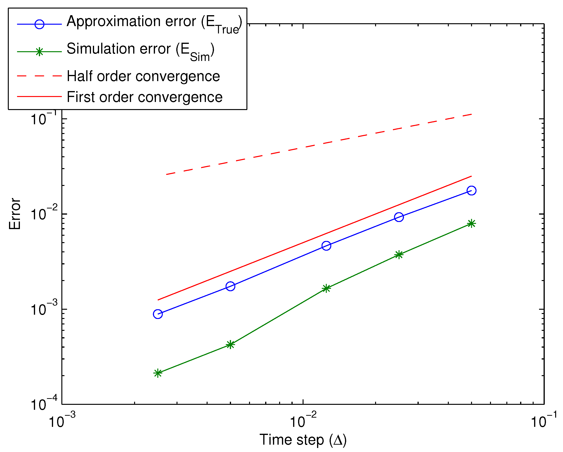
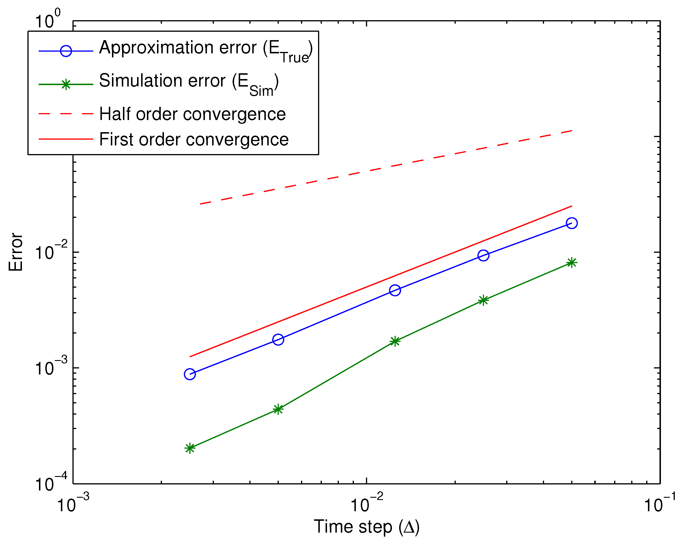
We systematically use m = 1000 paths. Even if the errors E T r u e and E S i m may be of the same order, they are interpreted differently. The error E T r u e gives the behaviour of the maximal approximation error on the grid whereas E S i m gives the behaviour of the error on the relevant part of grid when solving the FBSDE numerically. Figure 2 displays the errors under the explicit 1 stage Runge–Kutta scheme with n { 5 , 10 , 20 , 50 , 100 } and Figure 3 shows the errors under the explicit 2 stage scheme.
The error graphs of Figure 2 and Figure 3 look almost identical and confirm that the 2 stage scheme is of first order and the 1 stage scheme of (at least) half-order. The extra-efficiency of the 1 stage scheme may be attributed in this particular case to the simplicity of the driver f and the terminal condition g.
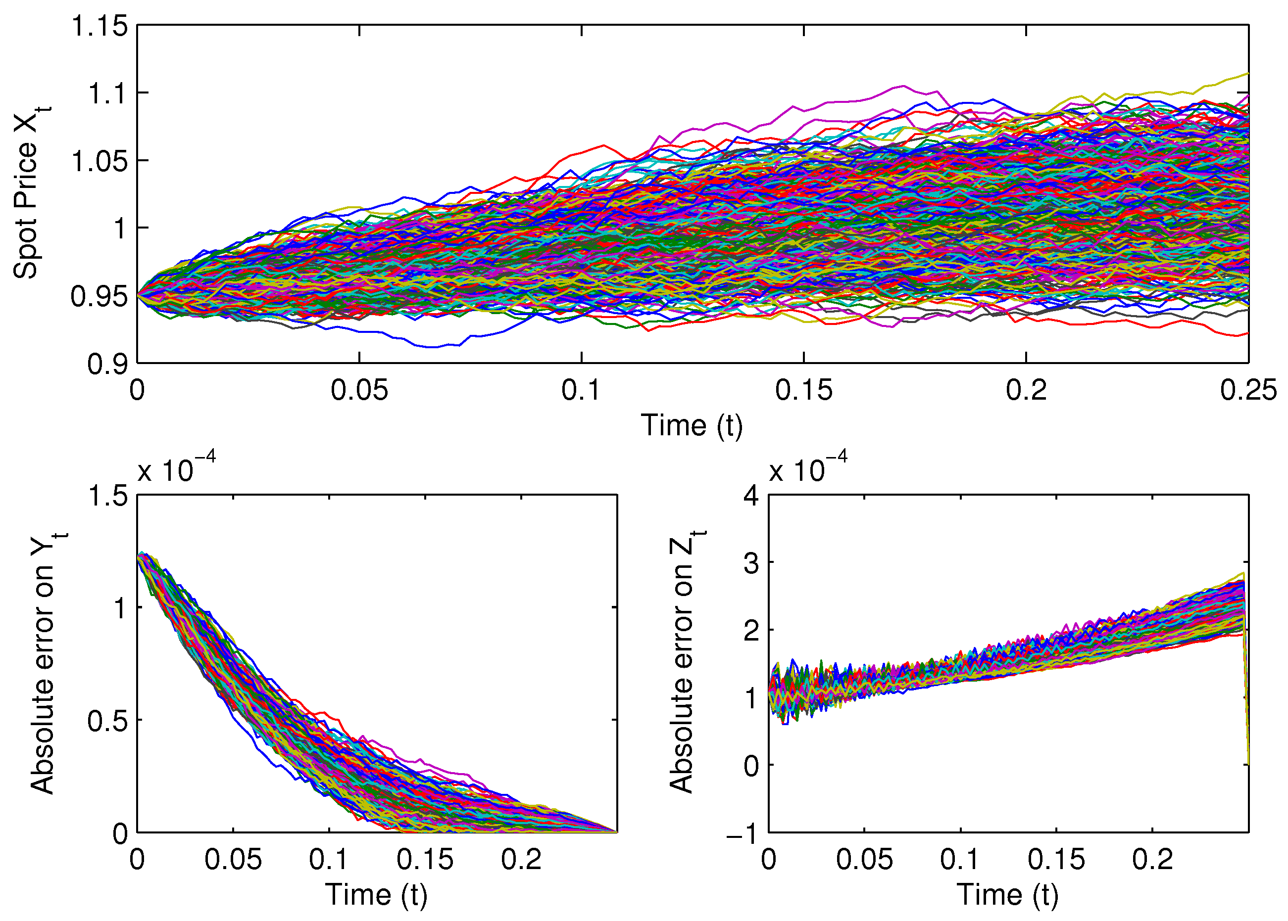
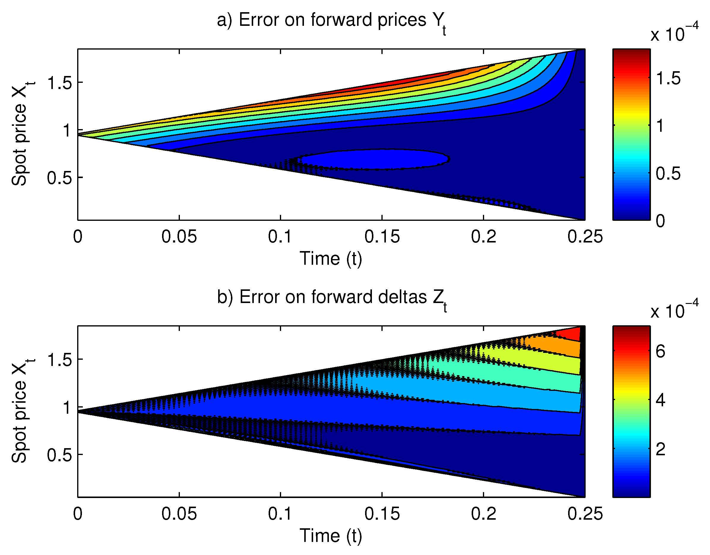
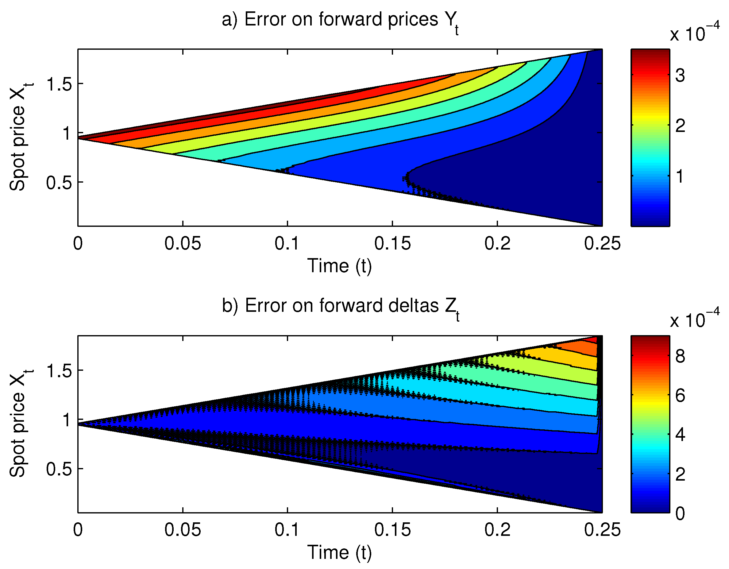
In Figure 4, we present the absolute errors along the simulated paths for the BSDE solution. One notices that the maximal errors occur at the initial time t 0 = 0 for the forward price ( Y t ) and at maturity T = 0.25 for the control process ( Z t ). Nonetheless, the simulation errors are of the same order ( 10 4 ) for both processes. This information is confirmed by the contour plot of Figure 5 not only along the simulated paths but on the entire grid.
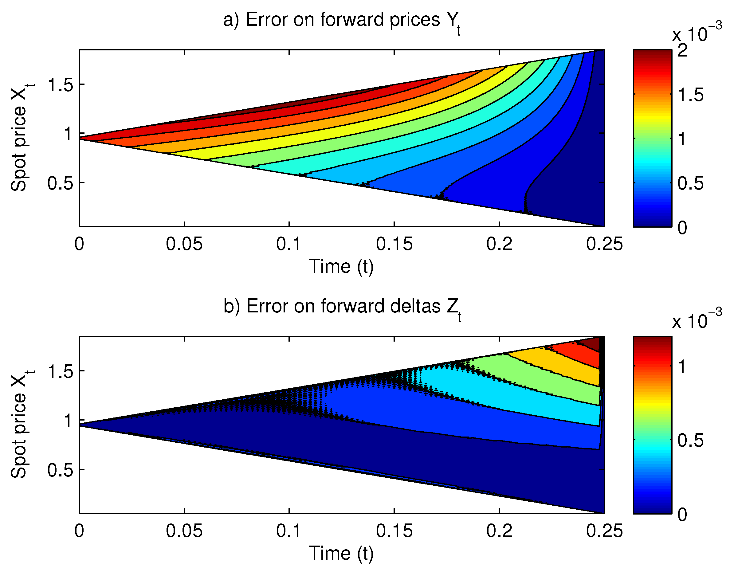
Moreover, the contour plot gives indication on the source of errors. Indeed, Figure 5 shows that the maximal errors mainly occur for the upper space node values on the alternative grid and they decrease for lower space node values. This is due to the unbounded nature of the spot price process coefficients. Since the volatility of the spot price is a positive and increasing function of the spot price4, higher spot price values lead to higher local volatility. Hence, the fixed length of increment interval l may not be sufficiently large to ensure accuracy for higher space node values. In general, the phenomenon is amplified with the magnitude of the forward process coefficients as illustrated in the contour plot of Figure 6 where we choose a higher value for the volatility σ and keep the other parameters unchanged. Similar results can be obtained by selecting a higher value for the speed of adjustment κ as shown in Figure 7.
We end this section with an efficiency study of our schemes. Using the parameters initially given, the BSDE is solved on a uniform time grid with n { 10 , 20 , 40 , 50 , 60 , 80 , 100 } time steps and N { 2 , 2 2 , 2 3 , 2 4 } space steps and value the computation time. Figure 8 displays the results. First note that since the Fourier interpolation method performs matrix multiplications, it is much slower than the convolution method of Hyndman and Oyono Ngou (2017).
As shown in Figure 8, the computation time of Fourier interpolation method increases with the number of time steps leading to a trade-off between computation speed and accuracy. The exponential nature of the curves suggests that preference has to be given to the coarsest time discretization providing a satisfactory level of accuracy. Similarly, the computation time also increase drastically with the number N of space steps. Coarse space grids insuring accuracy are hence also preferable. Since a total number of 2 q conditional expectations are computed under a q-stage Runge–Kutta scheme, we can expect the 1-stage scheme to run twice as fast as the 2-stage scheme. This is confirmed on Figure 8, especially when looking at the computation times for n = 100 .

5. Conclusions

In order to solve the problem of extrapolation errors in the initial implementation of the convolution method, we proposed an alternative space discretization. The new tree-like space grid naturally allows the usage of the FFT algorithm when computing the conditional expectation included in the underlying explicit Euler scheme. The error analysis shows that both the alternative grid and the (alternative) transform suit the periodic nature of the FFT algorithm and help in producing a stable, consistent and globally convergent numerical procedure for the FBSDE approximate solutions. The second part of the paper deals with the implementation of the Fourier interpolation method with higher order time discretizations of FBSDEs. When the forward process increments admit conditional characteristic functions satisfying certain regularity conditions, it was shown that the method is also consistent, conditionally stable and globally convergent under Runge–Kutta schemes for FBSDEs. A challenging area of research is the implementation of the methods of this paper in multidimensional and jump cases.
References [custom]

Author Contributions

Conceptualization, methodology, and writing: P.O.N. and C.H. Formal analysis, investigation, data curation and coding: P.O.N. Funding acquisition, supervision, review and editing: C.H. All authors have read and agreed to the published version of the manuscript.

Funding

This research was supported by the Natural Sciences and Engineering Research Council of Canada (NSERC) grant RGPIN-2015-04125.

Data Availability Statement

Not applicable.

Acknowledgments

The authors thank the anonymous referees for their helpful comments which improved the paper.

Conflicts of Interest

The authors declare no conflict of interest.

Notes

1
This approach was suggested by an anonymous referee of an earlier version of this paper.
2
The minimum sampling rate to avoid aliasing.
3
The real value P ¯ can be considered as the production cost (per unit) of the commodity.
4
See Equation (144).

References

  1. Bally, Vlad, and Gilles Pagès. 2003. A quantization algorithm for solving multidimensional discrete-time optimal stopping problems. Bernoulli 9: 1003–49. [Google Scholar] [CrossRef]
  2. Bally, Vlad, Gilles Pagès, and Jacques Printems. 2005. A quantization tree method for pricing and hedging multidimensional American options. Mathematical Finance 15: 119–68. [Google Scholar] [CrossRef]
  3. Beck, Christian, Weinan E, and Arnulf Jentzen. 2019. Machine learning approximation algorithms for high-dimensional fully nonlinear partial differential equations and second-order backward stochastic differential equations. Journal of Nonlinear Science 29: 1563–19. [Google Scholar] [CrossRef]
  4. Bender, Christian, and Jianfeng Zhang. 2008. Time discretization and Markovian iteration for coupled FBSDEs. The Annals of Applied Probability 18: 143–77. [Google Scholar] [CrossRef]
  5. Bender, Christian, and Robert Denk. 2007. A forward scheme for backward SDEs. Stochastic Processes and Their Applications 117: 1793–812. [Google Scholar] [CrossRef]
  6. Bouchard, Bruno, and Nizar Touzi. 2004. Discrete-time approximation and Monte-Carlo simulation of backward stochastic differential equations. Stochastic Processes and Their Applications 111: 175–206. [Google Scholar] [CrossRef]
  7. Briand, Philippe, Bernard Delyon, and Jean Mémin. 2001. Donsker-type theorem for BSDEs. Electronic Communications in Probability 6: 1–14. [Google Scholar] [CrossRef]
  8. Chassagneux, Jean-François, and Dan Crisan. 2014. Runge-Kutta schemes for BSDEs. The Annals of Applied Probability 24: 679–720. [Google Scholar]
  9. Chevance, David. 1997. Numerical methods for backward stochastic differential equations. In Numerical Methods in Finance. Edited by Leonard Christopher Gordon Rogers and Denis Talay. Publications of the Newton Institute. Cambridge: Cambridge University Press, pp. 232–44. [Google Scholar]
  10. Crisan, Dan, and Konstantinos Manolarakis. 2012. Solving backward stochastic differential equations using the cubature method: Application to nonlinear pricing. SIAM Journal on Financial Mathematics 3: 534–71. [Google Scholar] [CrossRef]
  11. Crisan, Dan, and Konstantinos Manolarakis. 2014. Second order discretization of backward SDEs and simulation with the cubature method. The Annals of Applied Probability 24: 652–78. [Google Scholar] [CrossRef]
  12. Crisan, Dan, Konstantinos Manolarakis, and Nizar Touzi. 2010. On the Monte Carlo simulation of BSDEs: An improvement on the Malliavin weights. Stochastic Processes and Their Applications 120: 1133–58. [Google Scholar] [CrossRef] [Green Version]
  13. Delarue, François, and Stéphane Menozzi. 2006. A forward-backward stochastic algorithm for quasi-linear PDEs. The Annals of Applied Probability 16: 140–84. [Google Scholar] [CrossRef]
  14. Douglas, Jim, Jr., Jin Ma, and Philip Protter. 1996. Numerical methods for forward-backward stochastic differential equations. The Annals of Applied Probability 6: 940–68. [Google Scholar] [CrossRef]
  15. Duffie, Darrell, and Larry G. Epstein. 1992. Stochastic differential utility. Econometrica 60: 353–94. [Google Scholar] [CrossRef]
  16. E, Weinan, Jiequn Han, and Arnulf Jentzen. 2017. Deep learning-based numerical methods for high-dimensional parabolic partial differential equations and backward stochastic differential equations. Communications in Mathematics and Statistics 5: 349–80. [Google Scholar] [CrossRef]
  17. E, Weinan, Jiequn Han, and Arnulf Jentzen. 2022. Algorithms for solving high dimensional PDEs: From nonlinear Monte Carlo to machine learning. Nonlinearity 35: 278–310. [Google Scholar] [CrossRef]
  18. E, Weinan, Martin Hutzenthaler, Arnulf Jentzen, and Thomas Kruse. 2019. On multilevel Picard numerical approximations for high-dimensional nonlinear parabolic partial differential equations and high-dimensional nonlinear backward stochastic differential equations. Journal of Scientific Computing 79: 1534–71. [Google Scholar] [CrossRef]
  19. El Karoui, Nicole, Étienne Pardoux, and Marie-Claire Quenez. 1997. Reflected backward SDEs and American options. In Numerical Methods in Finance. Edited by Leonard Christopher Gordon Rogers and Denis Talay. Publications of the Newton Institute. Cambridge: Cambridge University Press, pp. 215–31. [Google Scholar]
  20. El Karoui, Nicole, Shige Peng, and Marie-Claire Quenez. 1997. Backward stochastic differential equations in finance. Mathematical Finance 7: 1–71. [Google Scholar] [CrossRef]
  21. Gobet, Emmanuel, Jean-Phillipe Lemor, and Xavier Warin. 2005. A regression-based Monte Carlo method to solve backward stochastic differential equations. The Annals of Applied Probability 15: 2172–202. [Google Scholar] [CrossRef]
  22. Han, Jiequn, and Jihao Long. 2020. Convergence of the deep BSDE method for coupled FBSDEs. Probability, Uncertainty and Quantitative Risk 5: 5. [Google Scholar] [CrossRef]
  23. Huijskens, Thomas P., Marjon J. Ruijter, and Cornelis W. Oosterlee. 2016. Efficient numerical Fourier methods for coupled forward-backward SDEs. Journal of Computational and Applied Mathematics 296: 593–612. [Google Scholar] [CrossRef]
  24. Hyndman, Cody Blaine, and Polynice Oyono Ngou. 2017. A convolution method for numerical solution of backward stochastic differential equations. Methodology and Computing in Applied Probability 19: 1–29. [Google Scholar] [CrossRef]
  25. Kloeden, Peter E., and Eckhard Platen. 1992. Numerical Solution of Stochastic Differential Equations. Applications of Mathematics (New York). Berlin: Springer, vol. 23. [Google Scholar]
  26. Lucia, Julio J., and Eduardo S. Schwartz. 2002. Electricity prices and power derivatives: Evidence from the Nordic power exchange. Review of Derivatives Research 5: 5–50. [Google Scholar] [CrossRef]
  27. Ma, Jin, Jie Shen, and Yanhong Zhao. 2008. On numerical approximations of forward-backward stochastic differential equations. SIAM Journal on Numerical Analysis 46: 2636–61. [Google Scholar] [CrossRef]
  28. Ma, Jin, Philip Protter, Jaime San Martín, and Soledad Torres. 2002. Numerical method for backward stochastic differential equations. The Annals of Applied Probability 12: 302–16. [Google Scholar]
  29. Oyono Ngou, Polynice. 2014. Fourier Methods for Numerical Solution of FBSDEs with Applications in Mathematical Finance. Ph.D. thesis, Concordia University, Montréal, QC, Canada, January. [Google Scholar]
  30. Pardoux, Étienne, and Shige Peng. 1992. Backward stochastic differential equations and quasilinear parabolic partial differential equations. In Stochastic Partial Differential Equations and Their Applications (Charlotte, NC, 1991). Lecture Notes in Control and Information Sciences. Berlin: Springer, vol. 176, pp. 200–17. [Google Scholar]
  31. Peng, Shige, and Mingyu Xu. 2011. Numerical algorithms for backward stochastic differential equations with 1-d Brownian motion: Convergence and simulations. ESAIM: Mathematical Modelling and Numerical Analysis 45: 335–60. [Google Scholar] [CrossRef]
  32. Ruijter, Marjon J., and Cornelis W. Oosterlee. 2015. A Fourier-cosine method for an efficient computation of solutions to BSDEs. SIAM Journal on Scientific Computing 37: A859–89. [Google Scholar] [CrossRef]
  33. Ruijter, Marjon J., and Cornelis W. Oosterlee. 2016. Numerical Fourier method and second-order Taylor scheme for backward SDEs in finance. Applied Numerical Mathematics 103: 1–26. [Google Scholar] [CrossRef]
  34. Turkedjiev, Plamen. 2015. Two algorithms for the discrete time approximation of Markovian backward stochastic differential equations under local conditions. Electronic Journal of Probability 20: 1–49. [Google Scholar] [CrossRef]
  35. Vašíček, Oldřich. 1977. An equilibrium characterization of the term structure. Journal of Financial Economics 5: 177–88. [Google Scholar] [CrossRef]
  36. Zhang, Jianfeng. 2004. A numerical scheme for BSDEs. The Annals of Applied Probability 14: 459–88. [Google Scholar] [CrossRef]
Figure 1. Examples of alternative grids.
Jrfm 15 00388 g001
Figure 2. Log-log plot of errors using the 1-stage Runge–Kutta scheme. The sample standard deviation of the error E S i m was less than 2 × 10 6 for all time discretizations.
Jrfm 15 00388 g002
Figure 3. Log-log plot of errors using the 2-stage Runge–Kutta scheme. The sample standard deviation of the error E S i m was less than 2 × 10 6 for all time discretizations.
Jrfm 15 00388 g003
Figure 4. Simulation errors using the 2-stage Runge–Kutta scheme. The numerical solution is obtained on a time mesh with n = 100 time steps and returns an forward price of 1.0121 and initial value of 0.0453 for the control process. The exact values are 1.0123 and 0.0452 , respectively.
Jrfm 15 00388 g004
Figure 5. Contour plot of errors using the 2-stage Runge–Kutta scheme. The numerical solution is obtained on a time mesh with n = 100 time steps and returns an forward price of 1.0121 and initial value of 0.0453 for the control process. The exact values are 1.0123 and 0.0452 , respectively.
Jrfm 15 00388 g005
Figure 6. Errors using the 2-stage Runge–Kutta scheme with σ = 0.08 . The numerical solution is obtained on a time mesh with n = 100 time steps and returns an forward price of 1.0115 and initial value of 0.0558 for the control process. The exact values are 1.0119 and 0.0556 , respectively.
Jrfm 15 00388 g006
Figure 7. Errors using the 2-stage Runge–Kutta scheme with κ = 3 . The numerical solution is obtained on a time mesh with n = 100 time steps and returns an forward price of 1.0238 and initial value of 0.0316 for the control process. The exact values are 1.0257 and 0.0315 , respectively.
Jrfm 15 00388 g007
Figure 8. CPU time (in seconds) of Runge–Kutta schemes.
Jrfm 15 00388 g008
Publisher’s Note: MDPI stays neutral with regard to jurisdictional claims in published maps and institutional affiliations.