1. Introduction
The mean variance analysis developed by
Markowitz (
1952) has been accepted as a paradigm for portfolio selection. The investment risk is measured by the variance of portfolio returns, following the normality assumption for asset returns. Not only has the normality assumption made the implementation of portfolio investment convenient, but also it has a strong economic theory on which the celebrated Capital Asset Pricing Model (
Sharpe 1964) is founded. However, this mean variance model usually results in large portfolio turnovers because the underlying data-generating process is far from normal, which limits its applicability to dynamic investment strategies. The mean variance analysis also performs poorly in out-of-sample tests, which supports that asset returns may be asymmetrical or non-normal and a different measure of uncertainty is required to characterize asset returns over time.
There are two components to consider in portfolio construction: (i) the price dynamics of the available investment opportunities; (ii) the decision model, which controls the returns on investment. So, the first step in building a portfolio investment model is to characterize the return and risk profile of financial instruments. There are good economic reasons why the equilibrium distribution of asset returns is conditional on the state of the financial market. The Internet bubble in 2001–2003, the subprime housing loan crisis in 2008–2009, and the recent COVID-19 pandemic market crash in early 2020, exposed severe limitations of the traditional mean variance investment model which ignores the economic strength of the market.
The key idea for characterizing financial market dynamics using a hidden Markov model is to resolve the issue of unobserved financial market strength. Financial instruments often exhibit different risk levels in various market situations. Hidden Markov models are capable of capturing abrupt changes in a mechanism that generates the data. Usually, regime categorization is linked to financial market sentiments. However, there is no clear determination as to whether the financial market is bearish or bullish through direct observations of the market activities. We sometimes observe a temporary rally in a bear market and a short period of slump in a bull market. With a hidden Markov model, investors have a better understanding of the market situation by applying Bayesian analysis to update the probability distribution of regimes with dynamically observed new information over time.
Many researchers have applied this approach to financial decision-making.
Hamilton (
1989) successfully applied a two-regime hidden Markov model to the U.S. GDP data and characterized the changing pattern of the U.S. economy.
Cai (
1994),
Hamilton and Susmel (
1994), and
Gray (
1996) used variations of the standard hidden Markov process to describe the time series behavior of U.S. short-term interest rates.
Bekaert and Hodrick (
1993) documented regime shifts in major foreign exchange rates.
Schwert (
1989) considered that asset returns may be associated with either high or low volatility which switches over time.
Whitelaw (
2000) constructed an equilibrium model in which consumption growth follows a regime-switching process.
Ang and Bekaert (
2002) studied an international asset allocation model with regime shifts.
Guidolin and Timmermann (
2006,
2008) provided important economic insights on how investments vary across different market regimes.
Tu (
2010) provided a Bayesian framework for making portfolio decisions with regime-switching and asset pricing model uncertainty.
Liu et al. (
2011) applied a regime-switching model to analyze the select sector exchange-traded funds.
Ma et al. (
2011) constructed a portfolio selection model to maximize managers’ alpha subject to limited risk exposure in different regimes. This modeling approach has posed much flexibility in explaining the observed market behavior and activities.
Individual asset returns and risk are the inputs to a decision model which determines the proportional investments in assets at each time point. In this paper, we develop a regime-switching regression model for the prediction of individual asset risk and return profiles. In a traditional asset pricing model, such as
Sharpe (
1964),
Fama and French (
1993,
2015),
Carhart (
1997), and
Ross (
1976), observed asset returns are directly related to observed risk factors. In a hidden Markov model, asset returns may exhibit entirely different relationships with the predictors in different regimes. For example, future equity returns are expected to go up with an increase in the current volatility in support of the idea of the leverage effect; see
Christie (
1982),
Bekaert and Wu (
2000). Furthermore, future equity returns are expected to go down with an increase in the current volatility level in support of the idea of the volatility feedback effect; see
Whitelaw (
1994). In this paper, we assume that broad equity market returns and market volatility jointly characterize systematic risk. Individual asset return and risk profiles are established through a switching-regression model on the two market risk factors of the broad equity market return and volatility.
The decision criterion is as important as characterization of the risk and return profile. The base risk-return model for the approach in this paper is mean return and return variance within a specific market regime. An efficient model trades off risk for return with a portfolio of investments. Variance of portfolio returns has shortcomings as a risk measure, considering the non-normality of asset returns implied by the hidden Markov model; for a detailed reasoning, see the example presented in
Section 3. A more generic measure for assessing the risk or “amount of randomness” in portfolio returns is entropy, which is a well-known concept coming from information theory and originally developed by
Shannon (
1948). It quantifies the uncertainty/amount of randomness conveyed by a probability distribution, embedding all higher-order moments (
Cover and Thomas 2006) and taking the entire probability distribution into consideration when measuring investment risk.
Entropy has been applied to measuring portfolio risk (
Philippatos and Wilson 1972;
Ou 2005;
Xu et al. 2011;
Usta and Kantar 2011) or to option pricing (
Gulko 1999). Similar to a variance measure, an entropy measure also has the property of translation invariance, therefore, a target return/risk trade-off should be established (note: the target return is not necessarily the portfolio mean return under the proposed model in this paper). Our portfolio is constructed by minimizing entropy rather than the variance of portfolio return. The particular measure considered in this paper is the exponential Rényi entropy (
Rényi 1961). Minimum Rényi entropy portfolios have been studied (
Lassance and Vrins 2021). However, the optimal entropy portfolio in a hidden Markov market setting with controls on shortfall has not been considered. It will be noted that a target means the return is not a suitable constraint in a hidden Markov model setting with variance as a risk measure, and this paper will try to fill the gap with a target mean return being replaced with shortfall surplus and probability of shortfall constraints.
Another aspect of portfolio selection is the concern of wealth shortfall from a target. In a mean variance model, if individual asset returns jointly follow a multivariate normal distribution, the surplus and shortfall are evened out around the target return, with a shortfall probability of 0.5. However, this is not the case when asset returns are asymmetric as in the hidden Markov model we introduce in this paper. We impose the constraints that the wealth surplus is greater than or equal to the shortfall and the probability of shortfall is less than a target probability level (≤0.5). These constraints have a significant impact on the investments in individual assets, depending on the overall predicted market strength. The settings for the target return and shortfall probability are important. In the performance comparisons with other portfolio selection models, we will discuss how portfolio returns change by varying the target return and the probability of shortfall.
The rest of the paper is organized as follows.
Section 2 discusses a hidden Markov model for the dynamics of financial indicators and a regime-switching regression model for security returns.
Section 3 discusses the entropy and risk measurement with hidden Markov models. In
Section 4, we develop a dynamic entropy portfolio model with shortfall surplus and probability of shortfall constraints.
Section 5 presents the parameter estimation.
Section 6 analyzes portfolio performance with a varying target return and the probability of shortfall.
Section 7 presents the performance comparisons of the entropy-based model with other investment strategies.
Section 8 concludes the paper.
2. The Basic Financial Market Models
The financial market is a stochastic dynamic process. The state of the market or market sentiment is defined by the movements of fundamental economic indicators. The dynamics of asset prices are in turn affected by market sentiment and economic indicators. In this section, we discuss the structure of the financial market with two basic economic models. The first model characterizes the dynamics of embedded economic regimes in terms of the dynamics of fundamental indicators, and the second model defines the rate of return on assets within regimes through the relationship to indicators/factors. The intention is to present sound theoretical models for asset returns as well as equations that can be estimated from market observations.
2.1. A Hidden Markov Model for the Dynamics of Financial Market Regimes
Based on the changing patterns of economic indicators, financial markets are usually characterized by regimes, such as bullish and bearish, etc. These patterns among the economic indicators alternate with the economic situations over time. Stock markets may stay in a bullish regime for some time before moving to another regime at a later date. For example, during the Internet bubble period of 1998–2002, the stock market was extremely volatile, while market volatility was relatively low in the period of 2003–2006. It is highly probable that market sentiment, market volatility, and the non-smooth asset return processes are regime-dependent. We assume, therefore, that the dynamics of the financial market strength follow a hidden Markov model.
Suppose the financial market regimes follow a Markov chain,
, with a finite number of regimes, say
K, and a regime transition probability matrix
where
is the transition probability from regime
i at time
to regime
j at time
t, which is independent of time
t. The outcome of the regime process at each time is a distribution over the possible regimes. We assume that the dynamics of the Markov chain are embedded in a set of financial/economic indicators. Thus, the parameters for the hidden Markov chain can be estimated using either economic or financial market indicators, through which the prior and posterior probabilities of the regimes can be calculated under a Bayesian framework.
The Markov chain can be modeled either as observable or hidden. The National Bureau of Economic Research (NBER) Business Cycle Dating Committee maintains a chronology of the U.S. economy, which identifies the dates of peaks and troughs that characterize economic strength into one of two regimes, namely, expansion and contraction. A contraction is defined as “a significant decline in economic activity spread across the economy, lasting more than a few months, normally visible in real GDP, real income, employment, industrial production, and wholesale-retail sales”, and an expansion is defined as the other way around, depending on the substance of the observed change in important economic statistics, such as the real GDP and the unemployment rate. However, a period is not identified as an expansion or contraction unless the economy stays on similar economic activities for at least six months. In other words, if the economy changes its strength within less than six months, the regime of the dated period will not change, which creates errors in identifying regimes and measuring the performance of asset returns under different economic environments. Another instability is that NBER may retrospectively change a regime that was categorized as a specific regime in considering its past performance if a subsequent economic pattern continues for more than six months. With their unstable rules for the characterization of expansion/contraction regimes, financial security performance within a regime may be incorrectly measured. Due to such a categorization policy, economic strength and asset returns might be incorrectly measured over time.
Given these caveats, we consider that the regimes are latent, and a hidden Markov model is used to characterize the economic strength over time. We assume that the regimes are embedded in a set of financial market indicators, which jointly follow a hidden Markov process.
Denote
the set of selected financial indicators. We assume that
follows a regime-switching first-order autoregressive model:
where
is a standard multivariate normal random variable, and
,
, and
, are regime-dependent coefficients of the model (
1) given
. Hence, conditional on
and
, the one-period regime-dependent expected value and covariance matrix of
are
and
, respectively. It should be noted that model (
1) deviates from a standard hidden Markov model in which the “emissions” or the observed quantities are identically and independently distributed given a specific regime. Our observations in model (
1) are dependent on the one-step-back observations. However, the estimation process will be the same as that for the standard hidden Markov process, with the assumption that, for any two time points,
s and
t,
and
are independent.
The prior and posterior probabilities of the
K regimes at any point in time can be calculated using Bayesian updating. Let
be the prior probabilities of the
K regimes for time
t. The posterior probabilities,
, of the regimes at time
t are given by
where the likelihood
is the normal density function with mean vector
and covariance matrix
evaluated at the observation
for regime
k. The prior probabilities for time
are given as
The above Bayes updating under a time-varying financial market will be applied to dynamically forecasting an asset return/risk profile.
2.2. A Regime-Switching Regression Model for Asset Returns
Financial asset returns reflect the interaction of buying and/or selling activities, which creates uncertainty or risk in making investment decisions. By modeling the variation in asset returns, we can obtain insights into general patterns. The quality of the asset pricing model is an important component of risk. The accuracy of return predictions is strongly linked to business-cycle fluctuations. There exist a variety of states/regimes in the financial market, such as Bull, Slump, Bear, and Rally, etc. Based on the existence of regimes, we assume that the dynamic of financial market regimes follows a stochastic process, with the transitions between regimes determined by fundamental financial factors. Assuming current returns reflect available information, a Markov process is proposed for the dynamics of asset returns. Markov regime-switching models account for both the probability and the magnitude of future breaks by extracting unobserved information from the underlying switching process. A combination of predictive regression and regime-switching models has the potential to significantly improve return predictability (
Hammerschmid and Lohre 2018).
Ang and Bekaert (
2002,
2004) demonstrate the usefulness of regime switching in the context of asset allocation. Accounting for the regime structure in financial decisions is important since an investment portfolio designed for a specific market strength can perform poorly in a different regime.
Suppose that the investment opportunities consist of
n risky and one risk-free security. The one-period logarithmic returns on the risky assets follow a multivariate normal distribution given that the financial market is in a specific regime. Let
be the returns on the
n risky securities from
to
t, which are characterized by a regime-switching regression model,
where
,
, and
are regime-dependent parameters, i.e., given
,
is a vector of length
K,
is a matrix of size
, and
is a diagonal matrix of size
n, indicating that the idiosyncratic risks of the risky securities are uncorrelated.
is the risk-free return at time
t, and
is a standard normal random vector, which is serially independent and uncorrelated with
, given
. Hence, conditional on the regime at time
t and the observation of
, the
n asset returns jointly follow a multivariate normal distribution:
Models (
2) and (
3) imply that the regime-dependent mean returns of the risky securities are time-varying and depend on the information on the risk factors, while the regime-dependent covariance matrices are constant over time.
Based on the prior probabilities for regimes at each point in time, the unconditional returns of the risky securities follow a mixture of normal distributions with a mean vector,
and the covariance matrix,
The above calculated (unconditional) mean vector and covariance matrix will be the inputs to a mean variance model. The estimates calculated from (
4) and (
5), using HMM regime-specific estimates for means, covariances and probabilities, are a significant improvement on the estimates without multiple regimes.
3. Entropy and Risk Measurement
The fundamental concepts in assessing an investment strategy are risk and return. Risk is associated with uncertainty, and a measure that quantifies the uncertainty of a random variable
X reflected in its distribution is entropy. The entropy measure of a discrete random variable
X, introduced by
Shannon (
1948), is defined as
where
is the probability of
and
N is the size of the probability support
(
N can be infinity). Shannon entropy is generally used as a measure of information uncertainty. The larger the entropy, the more uncertain the
X.
For a continuous random variable
X, the entropy is naturally extended as
where
is the density function of
X. (
7) is usually called
differential entropy, which has many of the properties of discrete entropy. However, unlike the entropy of a discrete random variable, the differential entropy of a continuous random variable may be infinitely large, negative or positive (
Ash 1965). The entropy of a discrete random variable remains invariant under a change of variable; however, with a continuous random variable, the entropy does not necessarily remain invariant.
Shannon entropy is linked to variance—the usual measure of uncertainty. If
X is normally distributed with mean
and standard deviation
,
So, the differential entropy analogy of Shannon entropy (
Shannon differential entropy) is determined by the variance, and mean variance analysis is equivalent to a mean entropy approach if asset returns jointly follow a multivariate normal distribution. This gives us a hint that we may use entropy to measure a portfolio’s return variability or randomness.
For non-normal distributions, variance alone does not define entropy, so entropy is preferred as a measure of uncertainty since it takes the entire distribution into consideration. For non-normal distributions, the Shannon differential entropy is computationally intractable, and we introduce a tractable generalization of Shannon differential entropy.
In (
8),
Rényi (
1961) proposed a generalization of Shannon entropy with the following definition:
whenever the expectation exists. Shannon entropy is recovered as a special case in the sense that
The Rényi entropy in (
8) has a discrete analogy. If
X is a discrete random variable with distribution
, the Rényi entropy is
The Rényi entropy of a discrete random variable is non-negative. However, the Rényi entropy for a continuous random variable (
differential entropy) can be negative. Although the definitions are analogous, the functions have different ranges of values.
Tabass et al. (
2016) established that continuous case Rényi entropy is not the limit of Rényi entropy for discrete approximations. If the discrete approximation to
X is
, where
on the interval
and
, then
So, the limit of Rényi entropy for a quantized approximation of a continuous random variable does not converge to the differential entropy of a continuous random variable. Given this caveat, we will confine our entropy analysis to a continuous random variable with a density function.
It is known that, while the entropy of a discrete random variable is always non-negative by definition, the entropy of a continuous random variable can be negative. Since a risk measure is required to be a positive functional, the exponential transform of Rényi entropy has more natural properties in the context of risk. We denote by
the exponential Rényi entropy, which is
Note that exponential Rényi entropy is defined by variance in the normal case. The exponential Rényi entropy of
collapses to (
Koski and Persson 1992)
is in the form of a power utility function of the probability distribution, and it has attractive properties.
For a hidden Markov model, the one-period return follows a mixture of normal distributions and the density function is given as
where
is a multivariate normal density function with mean vector
and covariance matrix
, and
is the probability of regime
k,
.
With a normal mixture, the quadratic Rényi entropy has a closed form solution, as in Proposition 1. To simplify notation, we will denote as the exponential Rényi entropy with .
Proposition 1. The entropy of the mixture normal random variable, X, with a density function in (10), is given aswhere is the normal density function with mean 0 and variance evaluated at , . The explicit solution for quadratic Rényi entropy has computational advantages since the general entropy formula is difficult to calculate. It is also intuitively appealing since is composed of the within-regime means and covariances. As a risk measure, it also satisfies the properties as in Proposition 2.
Proposition 2. Let c be a real constant and X a random variable with a density function (10). satisfies the following properties, - 1.
Positivity: and the equality holds if X is a constant.
- 2.
Translation-invariance: ;
- 3.
Positive-homogeneity: .
Proof. The proof of Proposition 2 is straightforward by using the result in Proposition 1. □
Using the translation-invariance and positive-homogeneity properties, we can easily derive that the entropy of a constant equals zero. Unfortunately, the subadditivity for deviation risk measures does not hold in general for
with mixture normal distributions as in (
10), though it does hold for
with normal distributions (number of regimes equals one). For illustration, assume there are two regimes with a prior probability
.
X has parameters
and
, and
Y has parameters
and
. The correlation of
X and
Y for the two regimes are
. By Proposition 1,
,
, and
. Thus,
. However,
Rau-Bredow (
2019) argued that subadditivity is not always the desired property for measuring financial risk. That is, when two investment positions are merged, the resulting risk is actually even greater. As examples of subadditivity violation, the celebrated risk measure, Value-at-Risk (VaR), does not satisfy subadditivity, and the variance measure does not satisfy subadditivity either. Since we are measuring the randomness of a portfolio return, not concerning monetary risk, we will ignore the assumption of subadditivity in developing our portfolio selection model.
4. The Investment Model
The structure for the dynamics of asset prices has been proposed in
Section 2, and we will consider investment decisions based on that structure. An investment decision is a portfolio
, where
is the proportion of available capital allocated to risky asset
i,
, from time
to
t. The return on the portfolio is
where
is the risk-free return and
is the proportion allocated in the risk-free asset. It is assumed that there are
K regimes and, given
, the returns on the
n risky assets are multivariate normally distributed with mean vector
and covariance matrix
. Hence, given regime
,
is normally distributed with mean
and variance
Let
be the probability density of the one-period portfolio return, and let
be the prior probabilities of the regime at
t. Then, the density function of one-period portfolio return
where
is the normal density function with mean
and variance
for portfolio weight vector
. So the distribution of returns is a mixture of normals.
The reference investment model built on risk and return is mean variance analysis. With a mean variance analysis, if asset returns are normally distributed, it can be shown that the optimal solution is such that the target mean return is binding, and the probability of the portfolio return greater than or equal to the mean is equal to the probability that the portfolio return is less than or equal to the mean, and both are equal to 1/2. However, this optimal portfolio property is violated if asset returns are non-normal and the density function is asymmetric. Therefore, using a target mean constraint is sub-optimal in that case.
If the properties are an important consideration, then a key issue with non-normal random returns is whether a target mean return is desirable, though it is a convenient measure of central tendency and it is a linear operator. A disadvantage of the mean of a quantity is that it is not robust, especially, in the presence of substantial skewness or fat tails as in the financial data. For example, the probability for a non-normal random outcome to be around the mean may be an event with a small probability to occur, if the means of the mixing normals are far apart and/or the component standard deviations are small.
Example 1. Let us use an example to illustrate the problem with a target mean for a mixture of normal return distributions. Suppose there are two regimes with a prior probability of and the portfolio return R is a mixture of two normal distributions with mixing parameter p. There are two risky assets, which have a joint normal distribution with and for regime 1 and a joint normal distribution with and for regime 2. Thus, the joint return distribution of the two assets is given asThe risk-free rate . We can interpret that regime 1 is a bear market and regime 2 is a bull market. Suppose the target return is . The mean variance optimal portfolio weight vector is . It can be verified that the shortfall equals 0.1490 and the surplus equals 0.1299 with a shortfall probability of 0.4656. At optimality, the shortfall is greater than the surplus, though the shortfall probability is less than 0.5, which is unreasonable. Suppose now the prior probabilities of regimes , which indicates that the strength of the financial market is reversed, and everything else stays the same. The joint return distribution of the two assets is given asTo meet the target return level of , the mean variance optimal portfolio weight vector changes to . The portfolio shortfall equals 0.1138 and the surplus equals 0.1345 with a shortfall probability of 0.5415. As a result, the shortfall is less than the surplus, but the probability of shortfall is much greater than the probability of surplus. This is again unreasonable. In conclusion, the mean and variance trade-off is not the best criterion for portfolio selection with non-normal and/or asymmetric asset returns. Considering that the target return and shortfall probability are the quantities of interest, we will directly constrain them. For a target return , is the probability that portfolio return is less than or equal to . We call the shortfall probability from target , and the quantity, , is called surplus probability over target . The quantity, , is called the shortfall below target , and the quantity, the surplus over target .
Given the shortfall probability less than or equal to 0.5, it follows that surplus is greater than or equal to shortfall implying that the portfolio mean return is greater than or equal to
at optimality. We control the shortfall probability being less than some desirable level and simultaneously guarantee that surplus exceeds the shortfall. With shortfall/surplus constraints on returns and quadratic (collision) Rényi entropy as the risk measure, the optimization model for portfolio selection is defined as
where
is portfolio return for risky asset weighting
W and
is the probability density function of
. The first constraint controls the losses in expectation, and the second one limits the probability of losses to a target level of
, which can be fine-tuned depending on the prior probability distribution of future regimes and the target return level
. As mentioned, if
and portfolio return is normally distributed, the optimal problem reduces to a typical mean variance model.
As previously stated, the reference for the investment model in (
12) is the Markowitz mean variance model. Major theoretical results have followed from mean variance analysis including the Capital Asset Pricing Model. The CAPM equation is an equilibrium result if investment decisions are governed by the mean variance criterion. Is this equilibrium framework preserved if investors’ risk and return trade-off are based on entropy and return level? To answer this question, we are providing a simulation using the earlier example to verify the preservation of the CAPM equilibrium framework.
It is easy to calculate that the mean vector is
and the covariance matrix is
. For the mean variance model, the optimal portfolio weights in the risky assets are
Let
and
be the optimal portfolio weights in the two risky securities for (i)
—the mean entropy model (similar to the mean variance analysis) and (ii) q—the entropy model (
12) with the shortfall probability
.
Table 1 presents the optimal portfolio weights in the two risky securities for a range of target levels.
Dividing by the total weights of the optimal portfolio, the weights in the risky assets are the same for the 5 target return levels within each strategy. The optimal weights are [0.7878, 0.2122], [0.7657, 0.2343], and [0.3867, 0.6133], for , , and , respectively. This is to say that a two-fund separation applies. i.e., investors with different target return levels find their optimal portfolios of risk-free and risky assets by simply allocating their wealth to the risk-free asset and a portfolio of the risky assets, which is the same for all investors.
5. Parameter Estimation
The equations in the financial market have parameters that need to be estimated so that the portfolio models can be implemented. The parameters to be estimated are the initial probability distribution of regimes
, and the transition matrix
P of regimes,
in the hidden Markov model (
1), and
in the regime-switching regression model (
2).
5.1. The Data
Since the financial market regimes are latent, we employ a hidden Markov modeling framework for the estimation process using weekly historical data on multivariate economic and financial indicators.
Edirisinghe and Zhao (
2020) used a set of macroeconomic indicators to characterize the hidden Markov model, and
Maclean and Zhao (
2022) used two typical equity market real-time indicators: the S&P 500 index (SPX) and the monthly CBOE volatility index (VIX). It is expected that the financial market regime dynamics can be well characterized by these two risk factors. Specifically, the first factor is the equity excess return, denoted
, i.e., the weekly logarithmic return on the S&P 500 Return Index minus the risk-free rate, and the second risk factor is the logarithmic ratio of the weekly VIX, denoted as
.
Figure 1 depicts the cumulative weekly values of
for the period 31 December 1998–30 April 2022.
It is observed that SPX and VIX move in opposite directions in 957/1217 weeks with a sample correlation of . There were several major market events in the past three decades. The Internet bubble in the late 19s and early 20s caused the stock market downturn in 2001–2002 and then led to a bull market for the period 2003–2007 with an ensuing peak in October 2007. A subprime mortgage crisis leading to market slowdown started soon after the boom and continued until June 2009. The European sovereign debt crisis was in the period from 2011 to 2013. Since then, the equity markets have up-trended, except for a few months of downturn due to the Greek debt crisis, until 2019. At the onset of the COVID-19 pandemic, the stock market suffered a major dip in March 2020. Then the stock market suffered a major drawback due to inflation concerns. Therefore, the pre-December 2018 period provides a representative in-sample data period for HMM-based analysis of economic regimes and their transitions. The out-of-sample data period for portfolio analysis is chosen as 1 January 2019–30 April 2022.
5.2. Estimation of the Hidden Markov Model
Determining the optimal number of states (or regimes) involves the conflicting notions that more regimes achieve a better fit of the model, while it also leads to poor predictive power due to overfitting the data. We apply the Bayes Information Criterion (BIC) to determine the optimal number of regimes,
where
is the maximized logarithmic likelihood,
is the total number of free parameters and
T is the sample length. So there is a trade-off between the likelihood and the number of parameters.
For the number of factors
N and the number of regimes
K, the number of free parameters is
based on the regime model (
1). It is well known that the maximum likelihood
monotonically increases with the number of regimes, which does not help with model selection. With the BIC criterion, an optimal number of regimes can be derived.
Table 2 presents the various model estimation criteria by the number of regimes with the Expectation-Maximization algorithm (
Dempster et al. 1977).
Based on the criterion of minimizing the BIC, the optimal number of financial market regimes is
. The initial regime distribution is estimated as
and the transition probability matrix
P is estimated as in (
14).
The transition matrix is diagonally dominant, so the probability to remain in a regime once the process is in that regime is relatively high. This is consistent with the reality in which a market regime holds for an extended time. In the long run, the market stays in each of the regimes with a probability distribution of
.
With a hidden Markov process, it is found that the categorization method provides a different regime process compared with the NBER characterization, which may be an interesting research topic for financial market analysis.
Table 3 presents the in-sample parameter estimation for the hidden Markov model (
1).
The numbers presented in
Table 3 have profound importance in financial research. The B coefficients are a reflection of the concept of leverage effect and volatility feedback. In the research literature so far, the focus is on the single regime case in which future asset return is negatively correlated with current asset return and positively correlated with current volatility, while future volatility is negatively correlated with current volatility. With multiple regimes, the concept of leverage effect and volatility feedback is much more complicated and requires further investigation.
With the information about the HMM dynamics and the observations of SPX and VIX, we can now label the four regimes of the financial market with terms that we name the market strength. It is noted that the correlations between SPX and VIX are negative in all regimes. However, their mean values have different patterns in different regimes, which provides a basis for us to label these regimes. Since SPX has a positive mean and VIX has a negative mean with the lowest standard deviation in Regime 2, we can label Regime 2 as Bull. In Regime 3, SPX has a slightly negative mean and VIX has a negative mean with the second lowest standard deviation, we can label regime 3 as Rally. Similarly, we can label Regime 1 as Slump and label Regime 4 as Bear. That is, most of the time, the financial market is in Bull or Rally, with a total of 0.4647 + 0.3378 = 80.25% chance. It is usually true that SPX and VIX are negatively correlated with a sample correlation of (for the case of single-regime). However, for a multi-regime model, the correlations between SPX and VIX are asymmetric and also negative across regimes, with the smallest correlation of in the Bull with stock prices going up and VIX index going down and the largest correlation of in the Slump with stock price going down and volatility going up. Interestingly, the estimated transition probabilities from Bull to Rally and Bear, from Rally to Slump, and from Bear to Slump and Bull, are extremely small (close to zero), which is consistent with the financial market observation.
5.3. Estimation of Asset Return Parameters
Investment in ETFs has become a style for both institutional and individual investors, as they are already diversified portfolios with low management costs compared to standard mutual funds. Some brokers have removed trading costs completely for some of the popular ETF funds. The select sector exchange-traded funds (SPDRs), each offering diversification benefits within each sector: Consumer Discretionary (XLY), Consumer Staples (XLP), Energy (XLE), Financials (XLF), Health Care (XLH), Industrial Goods (XLI), Basic Materials (XLB), Technology (XLT), and Utilities (XLU), have drawn a great deal of investor-attention since their origin in late 1998. Real Estate (XLRE) and Communication Services (XLC) are two additional select sector ETFs, but they started in 2015 and 2018, respectively. As they started much later, we use two substitutes, namely Simon Property Group ETF (SPG) for Real Estate and Verizon Communications (VZ) for Communication Services.
The weekly asset risk/return profile is estimated using the weekly returns of the eleven ETFs with the in-sample data. Following the discussion of model (
2), the forecast of the asset return/risk profile can be explicitly expressed with a regime-switching regression model as below,
where
is a vector of weekly returns on the risky securities.
,
,
, and
are regime-dependent parameters.
is a multivariate standard normal random vector, and
is the risk-free return from period
to
t. With the estimated hidden Markov process (
1) and the posterior probabilities of regimes over time, we apply a weighted least square method for each of the regimes to estimate the regime-dependent parameters.
Table 4 presents the estimates of the return parameters for model (
15).
Dynamic optimization depends on the estimated return parameters. In practice, portfolio managers usually apply a moving window approach to forecasting asset risk/return profiles. However, this approach may not be stable and beneficial. If we assume the risk/return profile of an asset is time-varying, we may not rely on a wide window of data for the estimation purpose. However, a too narrow window of data may not be sufficient for the significance of the estimates. For simplicity of discussion, we do not update the parameter estimation for either the hidden Markov model (
1) or the asset pricing model (
2), even though it might bring a benefit if these parameters are updated over time.
Based on the estimated parameters in
Table 4, we can now calculate the conditional mean vectors, standard deviations, and correlation coefficients of security returns over time. As specified in Equation (
3), the conditional mean vectors of the security returns are time-varying, but their conditional covariance matrix is constant given a specific regime.
Table 5 presents the conditional mean returns and standard deviations of the 11 ETFs for the first week of the out-of-sample period in January 2019, given a regime.
Given a regime, the conditional correlation coefficients of the 11 ETFs are presented in
Table A1 in the
Appendix A.
It is noted that the mean returns are all small in magnitude with mixed signs and the standard deviations are quite large for a single regime market. This is because the returns are averaged out when there is only one market regime. For the multiple regime market, the mean security returns are all positive in the Bull regime and negative in the Bear regime, with the Bull regime having a much smaller risk than the Bear regime. However, the mean returns in the Slump and Rally regimes have mixed signs, with returns in the Rally regime being much smaller than those in the Slump regime, indicating different responses to unconsolidated market strength, in contrast with consolidated Bull and Bear regimes. The patterns of the volatilities for all securities are similar, with the Bull regime having the lowest volatility followed by Slump, Rally, and Bear regime.
6. Dynamic Minimum Entropy Portfolio Analysis
The financial market is determined by the parameter estimates from weekly observations between 31 December 1998–31 December 2018 on the factors (SPX, VIX) and returns on the 11 SPDRs. It is considered that the observed out-of-sample trajectory of weekly values between 1 January 2019–30 April 2022 on the factors (SPX, VIX) and returns on the 11 ETFs is sampled from the estimated market. At the start of out-of-sample week t, a decision is made on the investments in the 11 ETFs: . The available information to the decision maker is prior probabilities for the regimes and the weekly returns on assets by the regime. Recall that the prior probabilities and the observed factor values from the week () yield posterior regime probabilities at the end of that week, and those posterior probabilities and the transition probabilities give the prior probabilities for week t. So the regime priors are dynamically updated each week.
The optimization model for portfolio selection is formulated as Equation (
12). The optimal portfolio
will produce actual portfolio returns from the observed returns on the assets in week t. The constraints in the entropy portfolio model (
12) have specifications for target return and shortfall probability. The model is applied with a variety of specifications to gauge the effect of the constraints.
6.1. Dynamic Portfolio Returns with Varying Target
It is noted that the risky assets have varying sensitivity to SPX and VIX with different magnitudes and signs, which create opportunities for constructing an optimal portfolio with combinations of long and short positions in the risky assets. This is consistent with one of the hedge fund investment styles, which has become popular among hedge fund portfolio managers. To make portfolio returns meaningful (without an absolutely large holding in some of the individual funds), we will set a target return equal to
where
r is the weekly risk-free return calculated from the 3-month LIBOR. To avoid large portfolio turnovers, the weekly risk premium is set to be small. For simplicity of exposition, we set the target probability of shortfall to be fixed and equal to 0.5.
Figure 2 depicts the cumulative returns and the total investment in the 11 risky assets.
It is shown in
Figure 2a that portfolio growth increases with target return, while it is shown in
Figure 2b that the net position of the portfolio weights in the risk assets are quite volatile as target return increases. Clearly, there is strong evidence of risk and return trade-off.
6.2. Dynamic Portfolio Returns with Varying Shortfall Probability
As elaborated previously, portfolio growth can change substantially by varying the maximum shortfall probabilities. It is desirable to control the probability of shortfall. However, a low probability of shortfall can make the optimization model infeasible if the required target return is high. With a weekly risk premium of 7 basis points,
,
Figure 3 presents portfolio returns and minimum entropy by shortfall probability at the level of
, and
.
It is observed that the lower the target probability level, the higher the portfolio entropy. It is also observed that the lower the allowable probability of shortfall, the higher the portfolio wealth growth, which clearly indicates the effectiveness of control on the maximum allowable probability of shortfall.
7. Comparisons with Alternative Portfolio Strategies
In this section, we discuss several investment strategies, which will be compared to the minimum entropy model. The basic approach with each strategy is to minimize portfolio risk subject to constraints on the portfolio return. The alternative models with which we are going to compare are the mean variance model with a single regime, the mean variance model with multiple regimes, the foresight strategy, minimizing entropy with a target mean return, and minimizing entropy with shortfall/surplus and shortfall probability constraints. As a review, these models are listed in
Table 6.
There are two design features in the alternative models: the asset pricing structure; the portfolio selection criteria. The mean variance models have the usual setting in which the portfolio variance is minimized subject to portfolio mean return being greater than or equal to a target return.
The contrast in pricing is a market with a single regime versus one with multiple regimes. In the case of a single regime, it is assumed asset returns follow a multivariate normal distribution. The mean variance analysis is implemented since the mean variance and mean entropy approaches are equivalent.
For multiple regimes, the basic assumption for a hidden Markov process is that, conditioned on the regime outcome at any point in time, asset returns follow a multivariate normal distribution. Each regime is associated with a different probability distribution for asset returns, which is expected to reduce the overall uncertainty of asset returns. There are two ways to proceed with switching regimes. Although the regime in the next planning period is not known, the Markov chain provides a “foresight” for predicting the future regime of the economy, using the prior probabilities of the regimes. The underlying data generating process assumes that one of the regimes is going to occur, so we may want to “guess” the future regime as the one with the highest prior probability, instead of using an “expected regime” approach. Let k be the most likely regime to occur, i.e., . This is a variation on the single regime approach, though the pricing parameter estimates are for regime k. The mean variance analysis is implemented with the returns for the single inferred regime. The argument here is that an “expected regime” will not occur, though the averaging over regimes accounts for the regime uncertainty.
In the case of multiple regimes and expectations over regimes, minimizing variance and minimizing entropy are different. So, both models subject to a target return are implemented.
For the model of minimizing entropy with a shortfall and surplus constraint, in addition to replacing the minimization of variance with minimization of entropy, we replace the usual mean target constraint with two constraints: (i) portfolio shortfall is less than or equal to the surplus and (ii) the probability of shortfall is less than a specific target level. Depending on the asymmetry of fund returns across all regimes, the target level of the probability can be fine-tuned so that, if the market is in a down regime, the probability level can be set tighter, so the portfolio will not put a large weight to avoid big losses. It can be easily proved that, with the constraint that portfolio mean return greater than or equal to the target return, if the shortfall probability is less than 0.5, the shortfall less than the surplus constraint will definitely hold. So, it is worth examining how the portfolio performs when the probability of shortfall is varied.
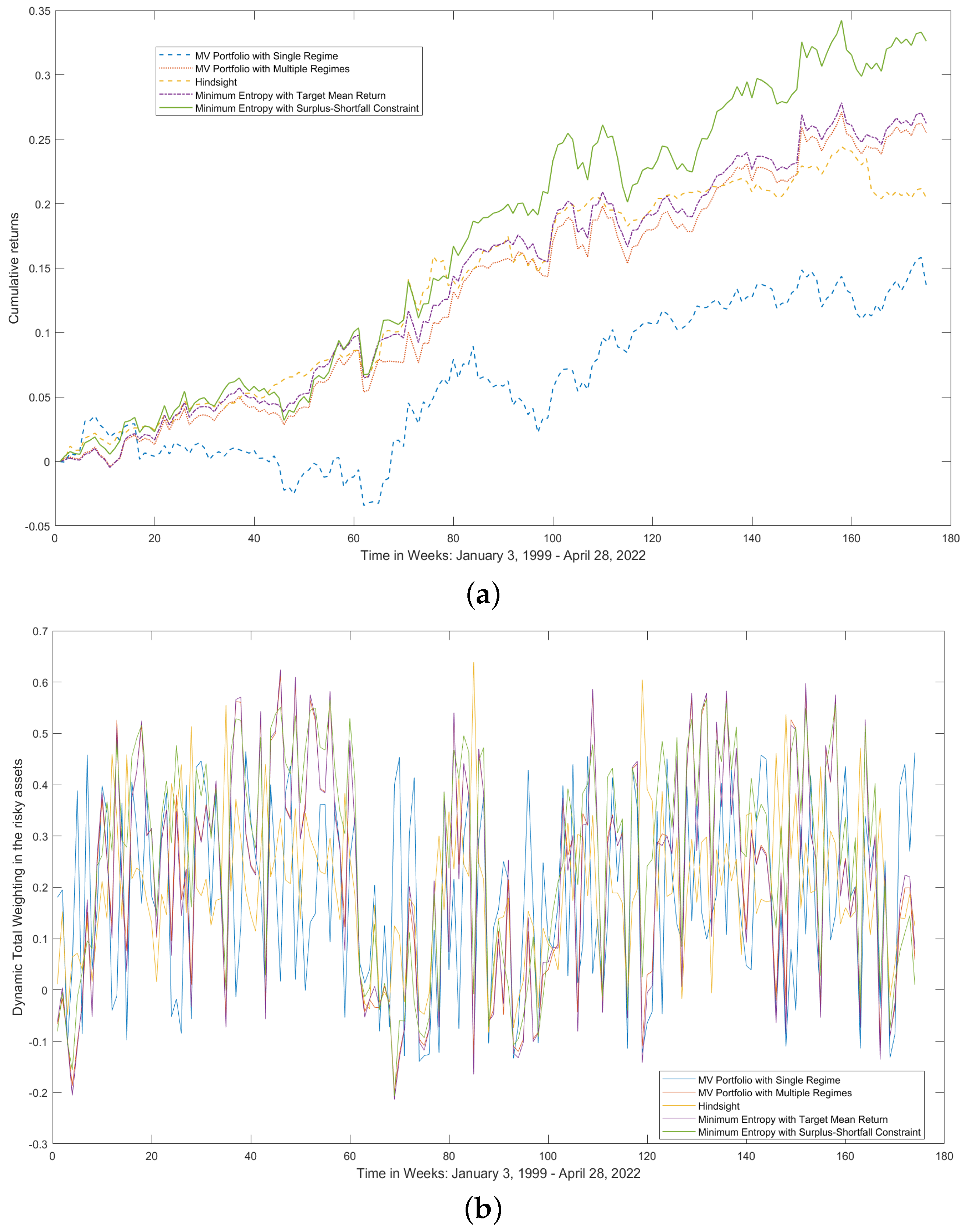
7.1. Cumulative Portfolio Returns and Net Weighting
Figure 4a,b depict cumulative portfolio returns and net weighting in the risky assets for the various investment strategies. In the portfolio comparisons, the shortfall probability is set to be 0.5, and the target return level is set to be the weekly risk-free returns plus 10 basis points.
From
Figure 4a, the mean variance model with multiple regimes, the foresight strategy, the minimum entropy with target return, and the minimum entropy with shortfall less than surplus outperform the mean variance model with a single regime, indicating a financial benefit of using a hidden Markov model for characterizing the dynamics of the equity market. The portfolio weight turnover is a concern for portfolio management. The net portfolio turnovers for all strategies are not so large as the risk premiums are set to be 10 basis points. Unexpectedly, it seems that the single-regime model has the highest portfolio turnover and the worst portfolio growth rate for the out-of-sample period.
7.2. Shortfall–Surplus Effect
The importance of controlling the surplus and shortfall over time was discussed previously and is a factor in cumulative returns.
7.2.1. Shortfall–Surplus Constraint
Figure 5 depicts the surplus-shortfall constraint binding/slackness.
From
Figure 5, the difference between shortfall and surplus for the single-regime model and the entropy model with shortfall constraint is always negative as discussed previously, while those for the mean variance model with a target return, the foresight strategy, and the entropy model, are changing signs over the sample period. It is also noted that the constraint has a similar pattern of slackness from
Figure 5, and they have a similar portfolio return pattern from
Figure 4a, indicating the importance of imposing the shortfall and surplus constraint.
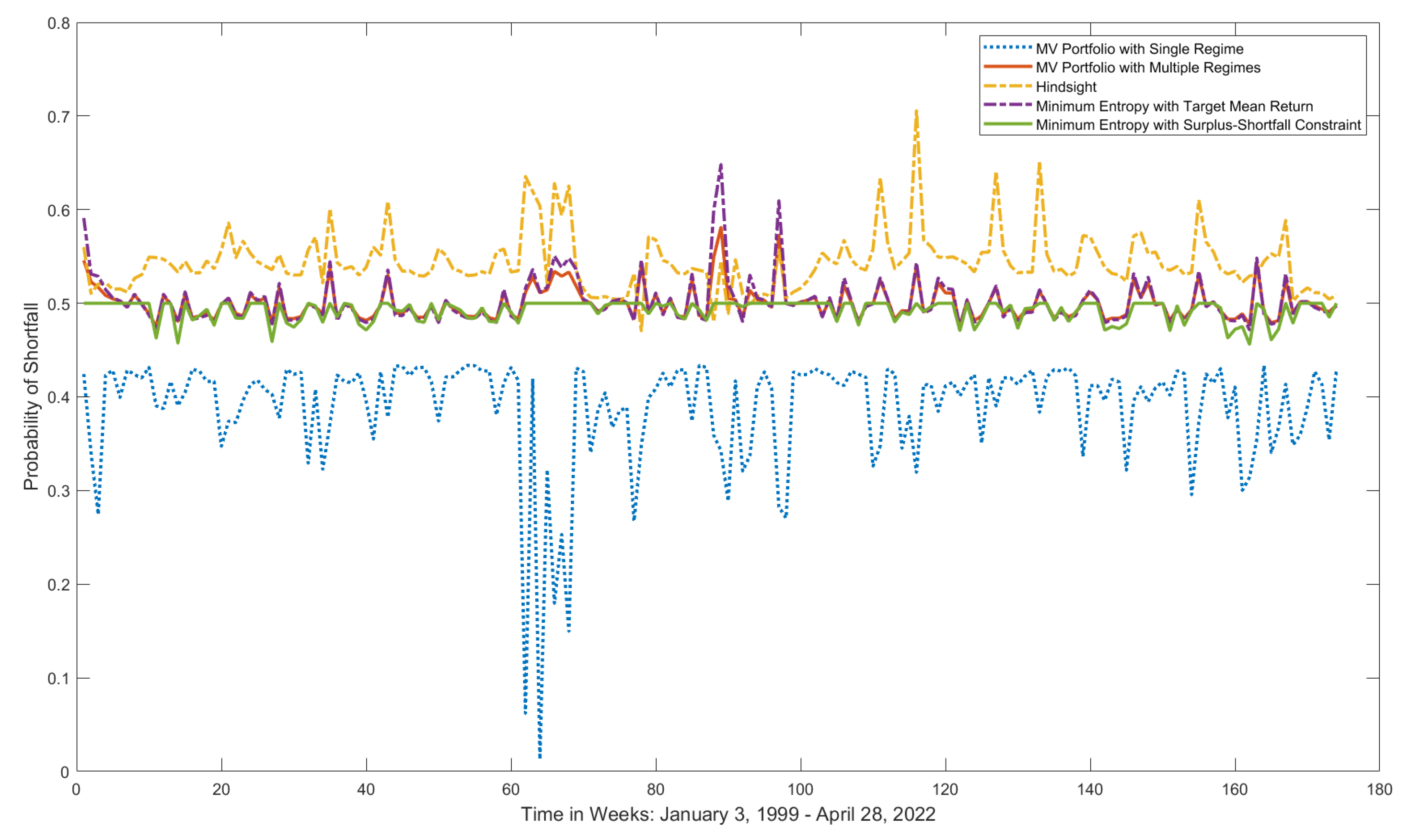
7.2.2. Shortfall Probability
From
Figure 6, we note that, at optimality, the estimated probability of shortfall for the single-regime model and the entropy model with shortfall probability constraint are both less than 0.5 as expected, while the other three models have an estimated shortfall probability being less than 0.5 some time and greater than 0.5 some other time, due to the asymmetric distribution of asset returns and in contrast with the single regime in which the probability of shortfall from the target return is automatically less than 0.5, assuming the target constraint is binding.
7.3. Summary of the Alternative Portfolio Performances
In addition to the period-by-period results presented in the figures included in this section,
Table 7 presents the overall results for the alternative portfolio strategies for the out-of-sample period.
It is shown that the S&P 500 index had the highest annualized growth rate of with the highest standard deviation of , which indicates that the overall equity market is volatile in comparison with the alternative strategies. The single regime model () had the lowest growth rate of 4.3705% with a substantial amount of risk of 7.2539% compared with other portfolio strategies. The mean entropy model () had a slightly greater mean growth rate with slightly lower volatility than the mean-variance model (), indicating a much more benefit in terms of risk and return trade-off using entropy as a risk measure. The foresight regime strategy () has the lowest volatility of 5.7129% among the alternative portfolio strategies, with a moderate growth rate of 6.7876%. Among all alternative portfolio strategies, our proposed model () had the highest growth rate of 11.5247% with a volatility of 8.7455%.
It is true that, with a single regime setting, the shortfall is always less than the surplus and the shortfall probability is always less than or equal to 0.5 for all alternative portfolio strategies. However, these properties are not preserved when asset returns are not normally distributed—such as proposed in this paper with a hidden Markov model as we discussed with a numerical example in
Section 4. For
, the mean shortfall is 0.4469%, the mean surplus is 0.4458%, and the shortfall probability is 0.4998%. For
, the mean shortfall is 0.4463%, the mean surplus is 0.4472%, and the shortfall probability is 0.5014%. It is evident that either
or
violated one of the two properties that a single regime model
preserved. However, strategy
is constrained to preserve these two properties simultaneously. From
Table 7, we also observed that the net investment exposures in the risky assets are quite low for all alternative strategies, ranging from 17.75% to 26.53%.
7.4. Performance Measurement
Portfolio performance is usually measured based on the portfolio’s historical returns. The most popular criterion is the sample Sharpe ratio which is the average excess return over the risk-free rate divided by its sample standard deviation, ignoring the return distribution. The Sharpe ratio may be suitable for normal portfolio returns, but it may not be so informative, as the portfolio return distribution changes over time and follows a mixture of normal distributions. To accommodate this, we provide a nonparametric approach for portfolio measurement using kernel density estimation.
Let
be the realized portfolio returns over a sample period. The following function is the kernel density estimation of the empirical density of the portfolio return
R:
where
K is the kernel (a simple density function) and
h is the bandwidth (a real positive number that characterizes the smoothness of the density function). The success of this nonparametric method depends on the choice of the kernel and the bandwidth
h. A too small bandwidth yields many kinks in the shape of the density, and a too big bandwidth increases the standard deviation. We choose a Gaussian kernel and the bandwidth selector developed by
Duong and Hazelton (
2005) to find the empirical portfolio return distribution.
Table 8 presents the empirical Sharpe ratios and the empirical mean entropy ratios of the alternative portfolios and the S&P 500 index.
From
Table 8, while the mean return of the S&P 500 Index is the greatest, it also has the largest standard deviation and entropy. It is shown that under both Sharpe and mean entropy ratios, the minimum entropy with shortfall–surplus and probability of shortfall constraints outperforms all other alternative strategies, which is strong evidence that the hidden Markov process has predictive power. It is worth noting that the foresight strategy has the smallest entropy and better performance than the single-regime mean variance model by both the Sharpe and mean entropy ratios, which implies that the hidden Markov model has a strong predictive power of the financial market strength.
8. Conclusions
In this paper, we argue that the standard mean variance model may not be a desirable investment criterion, given the existence of financial market regimes. The focus of this paper is to introduce an entropy-based portfolio selection model under a hidden Markov process. In addition to modeling portfolio risk with an exponential Rényi entropy, the main features of this portfolio selection process are the portfolio control with shortfall–surplus and probability of shortfall constraints. In contrast with alternative portfolio strategies, the strong portfolio performance of the entropy-based portfolio model is due to the uncertainty present in the regime-switching distribution of multi-regime asset returns, after accounting for the regime-dependent forecast of security returns.
Entropy-based portfolio selection is a relatively new concept, and it is now widely regarded as an attractive approach to creating portfolios with diverse exposure to a larger variety of securities. This paper provides a methodologically oriented and quantitatively rigorous approach to portfolio selection. Using factor models to characterize security risk/return profiles has been a trend in the investment arena. In this paper, we use the S&P 500 Return Index and the CBOE Volatility Index to model business cycles, and the empirical results presented a good fit to the reality with four regimes and compared well to the business states: Bull, Bear, Rally, and Slump.
The implementation in this paper considered a static approach in which the parameter estimation was not updated over time. Alternatively, a “dynamic” version may be envisaged in which the HMM is used to periodically update both the economic state (regime) distribution and the asset return parameters. That is, a moving time window of historical data of several periods may be used to update the asset return parameters prior to the portfolio rebalancing decision. We think such a dynamic implementation process may lead to a financial benefit.


