Net Impact of COVID-19 on REIT Returns

Abstract

Using an extended Fama–French model for REIT returns, we examine how the net impact of the COVID-19 pandemic differs from that of recessions. We find that, as anticipated, recessions have a negative net impact on office and residential REIT returns but that the COVID-19 pandemic has a positive net influence on industrial REIT returns because of e-commerce and the demand for storage, distribution, and shipping. Contrary to what we anticipated, there are no negative net effects of the COVID-19 pandemic on office and residential REIT returns, perhaps caused by both existing office and residential leases, the percentage rent clause for commercial properties, and the grace period for residential properties during the COVID-19 pandemic. In contrast to moving solely during recessions and the COVID-19 pandemic, we find that retail REIT returns fluctuate along with ongoing macro/asset-pricing conditions throughout the boom and bust cycle.

1. Introduction

The coronavirus pandemic, also known as the COVID-19 pandemic, was first discovered in Wuhan, China in December 2019, albeit its exact origin is still unknown. The U.S. reported the first case in January 2020, and declared the pandemic a public health emergency on 31 January 2020. On 11 March 2020, the World Health Organization (W.H.O.) declared the COVID-19 pandemic as a global pandemic.1 Governments around the world started to implement urgent measures to combat the spread of disease. Temporary closures of non-essential businesses, mask-wearing and social distancing requirements, and travel restrictions have resulted in substantial decreases in economic activity and employment. According to the Organization for Economic Co-operation and Development (OCED), the quarterly growth rate of real gross domestic product (GDP) in the U.S. experienced a dramatic decline from 0.5% in Q4 2019, to −1.3% in Q1 2020, to −8.9% in Q2 2020.2 The main drivers of these declines were substantial reductions in private final consumption and gross fixed capital formation.3 Meanwhile, the S&P 500 index fell about 32% between 10 February 2020 and 16 March 2020.4

The real estate sector in the U.S. is a hard-hit industry by the COVID-19 pandemic. There are substantial implications for real estate investment trust (REIT) investors. An REIT is a company that owns or finances income-producing real estate properties of various types. It is an important investment instrument for investors to get exposure to the real estate sector with flexibility and liquidity.5 The uniqueness of an REIT is the minimum required earnings payout ratio and the tax-exempt status at the corporate level. For a corporation to qualify as an REIT each year under the U.S. Tax Code, it must meet certain regulatory requirements regarding the organization structure, business operation, and distribution of income. For example, an REIT must invest at least 75% of total assets in real estate properties, earn at least 75% of gross income from rents generated from real estate properties, from interest payments generated from mortgages, or from proceeds from the sale of real estate properties, and distribute at least 90% taxable income in the form of dividends. Schnure et al. (2020) note that equity REITs offer greater compound annual returns compared to the S&P 500 Index over the 20-, 25-, and 30-year investment horizons through boom-and-bust circles. REITs are used as an effective hedge against inflation because the dividend growth of REITs would exceed inflation. Further, REITs are proven to be an asset class that can be added to a portfolio of stocks and bonds to enhance the return, and reduce the risk, of the resulting portfolio.

Would REITs behave differently this time during the COVID-19 pandemic from general recessions? In the literature on the COVID-19 pandemic and REIT returns, Ling et al. (2020) perhaps represents the first study on how regional exposure to the COVID-19 pandemic affects the U.S. REIT returns and find that the property type focus of an REIT, the geographic allocation of its properties, and the interaction between these two factors are the main contributors to this REIT’s return. Returns on retail, office, and residential REITs are negatively correlated with regional exposure to the pandemic while health-care and technology REITs are positively correlated with regional exposure. To the pandemic Milcheva (2022) assesses how the COVID-19 pandemic affects the risk–return relationship in the developed Asian (Hong Kong, Japan, China, and Singapore) and U.S. markets and finds sharp declines in average returns as well as a dramatic increase in market and idiosyncratic risks because of the COVID-19 pandemic. In the U.S. markets, REIT returns vary considerably across the property types but, in the Asian markets, REIT returns vary little across the property types. With this overall finding, the most significant under-performers are retail REITs in the U.S. and office REITs in Asia.

What the literature has omitted is the net impact of the COVID-19 pandemic relative to general recessions. The net impact is of interest because the recession induced by the COVID-19 pandemic is very different from the previous recession caused by the Global Financial Crisis (the GFC) during 2007–2009. First, to contain and fight the pandemic, policymakers restricted or suspended some economic activities immediately to prevent virus transmission and accelerated some other economic activities swiftly to provide essential goods and services. This would undoubtedly affect different economic activities abruptly across various real estate properties. Second, the policymakers needed to adapt quickly as they had gain better knowledge about the coronavirus and develop more effective vaccines and treatments. Third, the participation and cooperation of the public in policy measures were essential beyond the usual monetary and fiscal policy measures. Fourth, during the COVID-19 pandemic, the stock market fell from the peak in February 2020 to the trough in March 2020 and recovered literally in the same month. The rapid fall and recovery took a much shorter time relative to the historical stock market cycles. To fill the void, we attempt to examine how the net impact of the COVID-19 pandemic differs from that of general recessions.

Since required by law, equity REITs must earn at least 75% of gross income from the rent generated from real estate properties, the policy measures such as travel bans, remote working, the percentage rent clause for commercial properties, the grace period for residential properties, social distancing, and business lock-downs resulted in reductions and delays in rent collection. For example, hotel and motel and retail REITs were worst affected because of travel bans. The greater systematic risk for retail and residential REITs partially resulted from the percentage rent clause and grace period because landlords needed to share the risk of disruptions of cash inflows with their tenants (Gyourko and Nelling 1996). In addition, REITs are also required to distribute at least 90% (95% prior to 2000) net income to shareholders in the form of dividends to maintain the tax-exempt status. The requirement could reduce retained earnings and increase debt-financing without the tax-deductibility benefit considerably (Alhenawi 2011).6 The decline in cash flow affected the distribution of dividends and debt servicing in the short run. Consequential changes in cap rate, discount rate, and future cash flows had a significant impact on the fair value of real estate properties.The study in Akinsomi (2021) compares the year-to-date returns of REIT sectors in the U.S. in March and April 2020 relative to those in 2019 and finds that hotel and motel REITs experienced the greatest loss (−51.31%), followed by retail REITs (−48.74%). Office REITs and residential REITs both suffered a loss of around −20%. A loss of −10% was seen in industrial REITs. Data center REITs were the only REITs that witness gains of 8.8% in March and 17.66% in April, 2020 because data connectivity became essential when social distancing, remote working, and movement restrictions were widely practiced.

According to the National Association of Real Estate Investment Trust (NAREIT), commercial (office, retail, hotel and motel, industrial, data centers, etc.) real estate properties experienced a rising vacancy rates and falling rent growth in 2020, but exhibiting considerable variation across the property types, geographic locations, and qualities of properties. Office and retail REIT vacancy rates increased, respectively, from 9.9% and 4.7% in Q1 2020 to 10.7% and 5.0% in Q3 2020.7 However, unlike office and retail REITs, the increase (30 basis points) in industrial REIT vacancy rates was due to the elevated pace of construction and excessive supply despite the great demand for logistic spaces from the booming e-commerce transactions. Residential REIT vacancy rates were flat when the population had migrated from urban cores to suburbs and smaller cities because of the concerns about the pandemic and the practice of working from home (WFH). Valuation in the office and retail REITs fell by 3.8% and 3.2%, respectively, in Q3 2020 relative to Q3 2019. However, a steady rise was witnessed in multifamily residential and industrial REITs in the same quarter.8

Indeed, REIT returns fell during the recession induced by the COVID-19 pandemic. But we wish to go further to examine how the net impact of the COVID-19 pandemic differs from that of general recessions. In other words, we ask if the COVID-19 pandemic causes more damage to various REITs than general recessions do. We follow the chronology9 provided by the Business Cycle Dating Committee of the National Bureau of Economic Research (NBER). A recession is defined as the period between a peak of economic activity and its subsequent trough according to the NBER. During the GFC, economic contraction caused by internal weakness—excessive leverage, the overheated housing market, and financial crisis—is from December 2007 (Q4 2007) to June 2009 (Q2 2009), lasting for 18 months. The recent recession induced by the COVID-19 pandemic is from February 2020 to April 2020, lasting for only 2 months.

Using an extended Fama–French model, we find that recessions negatively affect office and residential REIT returns. We find that, as anticipated, due to e-commerce and the demand for storage, distribution, and shipping, the net impact of the COVID-19 pandemic on industrial REIT returns is positive. However, contrary to what we anticipated, the net impacts of the COVID-19 pandemic on office and residential REIT returns are not negative. This is perhaps caused by both existing office and residential leases, the percentage rent clause for commercial properties, and the grace period for residential properties during the COVID-19 pandemic. We find that retail REIT returns rise and fall together with continued changes in macro/asset-pricing conditions through the boom and bust cycle rather than only during both recessions and the COVID-19 pandemic.

We organize this paper as follows. Section 2 reviews the literature. Section 3 describes the data. Section 4 develops our hypotheses, model, and estimation/testing strategies. Section 5 analyzes the empirical results, Finally Section 6 provides concluding remarks.

2. Literature

There exists a considerable body of literature on the determinants for asset prices and returns. Ross (1976), Chen et al. (1986), and Roll and Ross (1995) view general economic variables as the determinants for asset prices and returns. Chan et al. (1990) show that the unexpected changes in inflation, term spread, and credit spread consistently drive equity REIT returns during the period of 1973–1987. Apparently, REITs as a special asset class are also exposed to these general economic variables. Redman and Manakyan (1995) examine the linkage between the risk-adjusted performance of REITs and financial and property characteristics during the period of 1986–1990 and find desirable geographic locations, ownership of health care properties, and investment in securitized mortgages can positively affect REIT returns.

Fama and French (1992, 1993) show that the stock return can be predicted by the market portfolio’s excess return (Rm-Rf),10 the size factor (SMB—Small Minus Big),11 the value factor (HML—High Minus Low),12 term spread (TSpread),13 and credit spread (CSpread).14 These factors are referred to as the macro/asset-pricing variables. Using the five-factor Fama-French model as in Fama and French (1993), Peterson and Hsieh (1997) find that returns on equity REITs are significantly correlated with Rm - Rf, SMB, and HML during the period of 1976–1992.

The literature also records a historical structural change in REIT pricing. The Revenue Reconciliation Act of 1993 was the dividing point between the vintage REITs eras during 1980–1992 and the new REITs eras starting from 1993 (Chiang 2015). Since 1992, an increase in analyst following and greater involvement of institutional investors help REIT share prices better reflect the performance of the underlying assets (Clayton and MacKinnon 2003). The correlation between REIT returns and the large-cap stock factor (the S&P 500 index) falls but that between REIT returns and the small-cap stock factor (the Russell 2000 index) or the real estate factor (the unsmoothed NCREIF total return index) rises in the 1990s. Emmerling et al. (2022) show that the performance behavior of RETs (Real Estate Trusts) is similar to that of REITs, especially with respect to financial crises (such as the Great Depression and the Great Recession). For REIT returns, we may extend the Fama–French model to include both the net impact of recessions and that of the COVID-19 pandemic. This allows us to infer if the net impact of the COVID-19 pandemic is more severe than that of recessions.

It is known that the financial position of an REIT mirrors its real business. Therefore, the expectations based on an REIT’s accounting data could affect its return. Chiang (2015) utilizes the conventional dividend discount model and shows a positive relationship between dividend yields15 and REIT returns. Although the contractual nature of rental leases has historically enabled REITs to pay dividends even during recessions, widespread dividend cuts during the GFC in 2008 indicate that the distribution of REITs dividends is not guaranteed and it depends considerably on the financial leverage and expected dividend payout ratio.16 For REIT returns, we may extend the Fama–French model to include relevant firm accounting variables.

Some unique accounting metrics are often used by REIT investors. Funds from Operations (FFO) and Net Income (NI) are two earning metrics used in analyzing REITs. FFO, a proxy for the REIT’s free cash flow, is defined as NI excluding gains (or loss) from sales of properties, plus non-cash depreciation and amortization, and adjusted for unconsolidated partnerships and joint ventures.17 FFO has been strongly promoted by NAREIT because of the implicit assumption that the value of real estate assets diminished predictably over time is embedded in the calculation of the GAAP performance metric NI (NI—historical cost depreciation). To supplement FFO, Adjusted Funds from Operations (AFFO) is regarded as a better metric for evaluating an REIT’s ability to pay dividends than FFO because non-cash amortized expenses are added back to, and recurring capital expenditures are subtracted from, NI. Schnure et al. (2020) indicate that REITs use the change in FFO, rather than in earnings per share (EPS) employed by non-REIT corporations, to measure earning growth. However, FFO and AFFO are not governed by the GAAP and are not audited. Vincent (1999) analyzes how changes in FFO and EPS affect market-adjusted returns and finds that both FFO and EPS consistently provide incremental information content. Using the long historical data, Emmerling et al. (2022) show that dividend growth rather than the discount rate drives real estate trust (RET) valuations. For REIT returns, we extend the Fama–French model to include firm accounting variables for profitability, liquidity, financial risk, and asset management.

3. Data

3.1. Quarterly Returns of Listed Equity REIT

There are 220 U.S. publicly-traded REITs listed and traded on the U.S. stock exchanges with a total capitalization of approximately U.S.$1.321 trillion in September 2021.18 Among these REITs, 95.2% or 180 REITs are equity REITs while 4.8% or 40 REITs are mortgage REITs.19 We focus exclusively on equity REITs and exclude mortgage, hybrid, healthcare facility, lodging/resort, diversified, specialty, hotel and motel, and real estate services REITs. We also exclude equity REITs for which full data are not available (For example, some REITs were taken over and merged with others whereas some REITs have very limited accounting data for our sample period). After these exclusions, we have the complete data for 20 office REITs, 12 residential REITs, 11 industrial REITs, and 24 retail REITs on the list of 67 equity REITs. The daily price data of 67 listed equity REITs from October 2007 to March 2020 are retrieved from Yahoo Finance using the R package “BatchGetSymbols”. To match the daily price data with these REITs’ quarterly accounting data, the quarterly return for each REIT is calculated by dividing the daily adjusted price (adjusted for dividends and stock splits) at the end of each quarter by the daily adjusted price at the start of each quarter minus 1 (quarterly return = $\frac{P_t}{P_{t-90}}-1$). The quarterly return statistics (mean, standard deviation, maximum, minimum, skewness, and kurtosis) of 67 equity REITs and their subgroup (office, residential, industrial, and retail REITs) quarterly return statistics (mean, standard deviation, maximum, and minimum) during the period of October 2007–March 2020 are calculated.20 Retail and office REITs deliver relatively low quarterly mean returns of $1.5336\%$ and $1.8879\%$, respectively, while residential and industrial REITs deliver relatively high quarterly mean returns of $2.9769\%$ and $3.5394\%$, respectively. The quarterly mean returns for retail and industrial REITs vary widely with the standard deviations of $21.74876\%$ and $17.3884\%$, respectively, while those for residential and office REITs vary less widely with the standard deviations of $15.2254\%$ and $16.7010\%$, respectively.

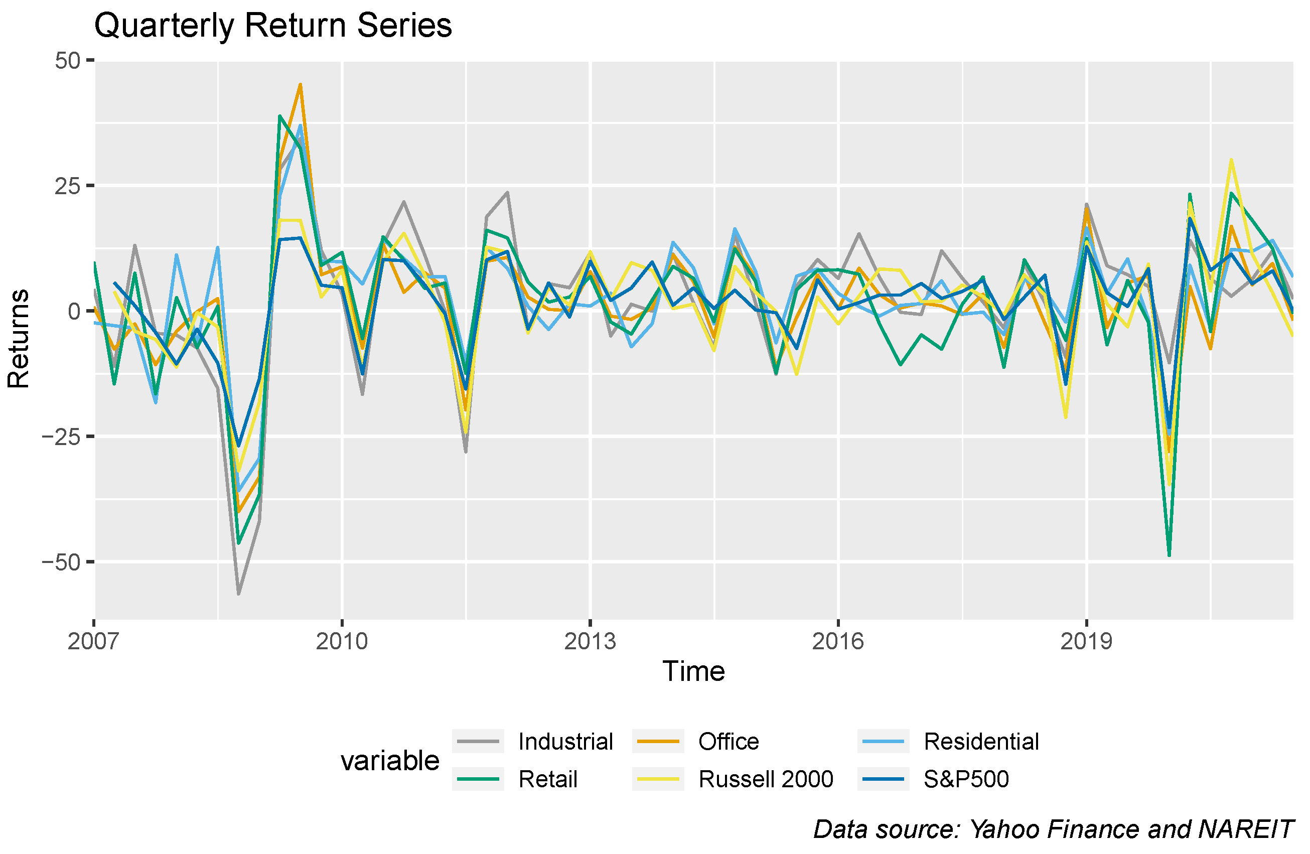
3.2. Main Market Indices and REIT Returns by Property Type

To show how the returns of different types of REITs and main market indices are correlated, we estimate the correlation coefficients among the quarterly total returns for the office, retail, industrial, and residential REIT indices from NAREIT, as well as the quarterly returns of the S&P 500 and Russell 2000 indices from Yahoo Finance. As shown in

Table 1. Correlation Coefficients among Main Market and REITs Indices Returns.

	Office	Retail	Industrial	Residential	S&P500	Russell 2000
Office	1.0000	0.9070	0.8574	0.9080	0.7797	0.7991
	(0.0000)	(0.0558)	(0.0682)	(0.0555)	(0.0829)	(0.0796)
Retail		1.0000	0.8043	0.8923	0.7683	0.7763
		(0.0000)	(0.0787)	(0.0598)	(0.0848)	(0.0835)
Industrial			1.0000	0.7788	0.8040	0.7375
			(0.0000)	(0.0831)	(0.0788)	(0.0895)
Residential				1.0000	0.6493	0.6641
				(0.0000)	(0.1007)	(0.0990)
S&P500					1.0000	0.9329
					(0.0000)	(0.0477)
Russell 2000						1.0000
						(0.0000)

Notes: The daily data of the S&P 500 and Russell 2000 indices during the period from January 2007 to November 2021 are retrieved from Yahoo Finance using the R package “BatchGetSymbol”. The daily return is calculated by the first log-difference of the daily adjusted price (for dividends and stock splits) [$log\left(\frac{P_t}{P_{t-1}}\right)=log(1+r)\approx r$]. Then the daily return then convert into the quarterly returns through ${\prod }_{t=1}^T(1+r_t)-1$. The monthly total returns of the FTSE Nareit U.S. office, retail, industrial, and residential REITs indices are retrieved from NAREIT.22 The monthly returns then convert into the quarterly returns. Each cell lists the correlation coefficient estimate and the standard deviation (in the parentheses).

, the correlation coefficient between retail and office REITs is high at 0.9070. Similarly, the correlation coefficient between retail and residential REITs is also high at 0.8923. The correlation between retail and industrial REITs is slightly lower at 0.8043. Similarly, the correlation coefficient between industrial and residential REITs is also slightly lower at 0.7788. In Table 1, we use the S&P 500 index for large-cap stocks in the U.S. and use the Russell 2000 for small-cap to mid-cap stocks in the U.S. As shown in Table 1, office, retail, and industrial REITs are highly correlated with these market indices while residential REITs are moderately correlated with these indices. This is consistent with the existing literature in that macroeconomic variables have predictive power for REIT returns (Clayton and MacKinnon 2003).

In Figure 1, we illustrate the fluctuations of REIT returns by the property type and their behaviors during the recessions caused by the GFC and the COVID-19 pandemic. As shown in Figure 1, retail REITs are among the least stable and most volatile property types of REITs during these recessions. The greatest price drawdown was witnessed in retail REITs during the COVID-19 pandemic and the magnitude of the price drawdown was more severe during the COVID-19 pandemic than during the GFC. However, as shown in Figure 1, industrial REITs behaved somewhat differently. They experienced the greatest drawdown during the GFC but were least affected by the COVID-19 pandemic. During the COVID-19 pandemic, industrial REITs were in high demand from the prevailing practice of remote working and movement restrictions, the high growth of e-commerce, and the increased need for warehousing and logistics. Office and residential REITs had less price drawdown than the Russell 2000 index did during the COVID-19 pandemic but more during the GFC.21

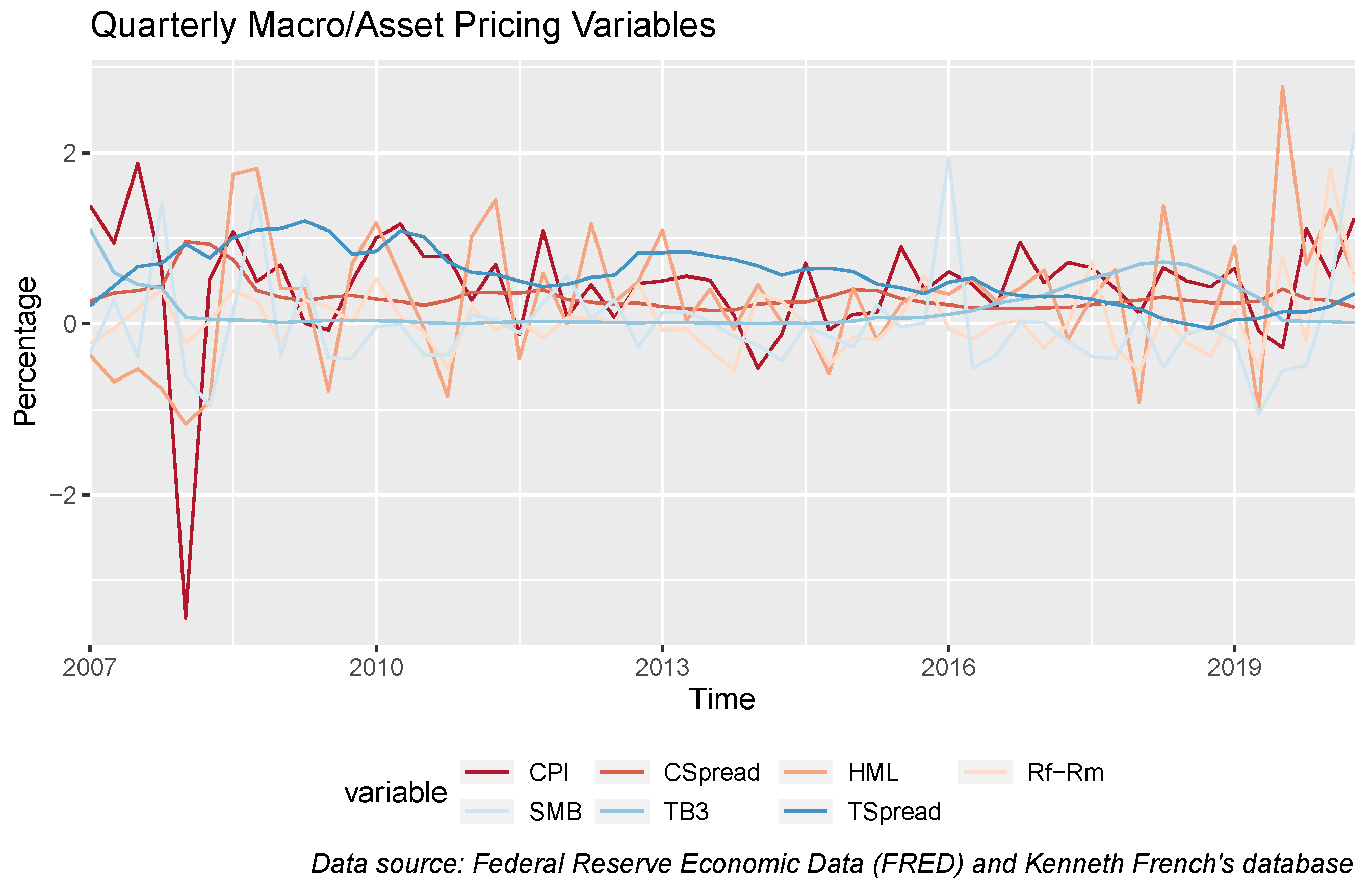
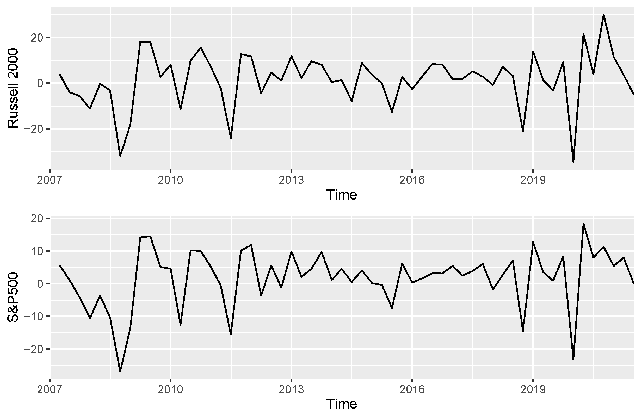
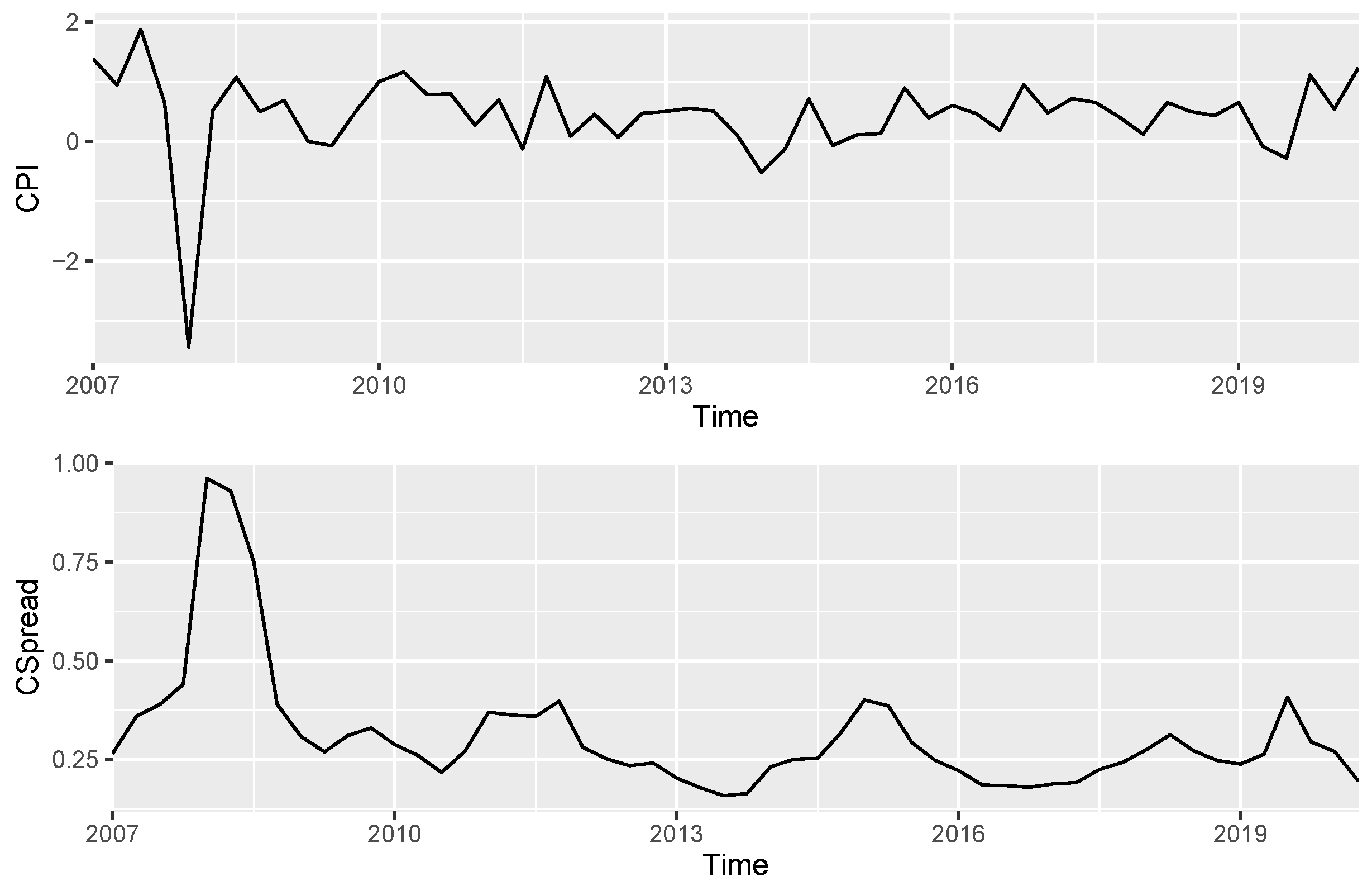
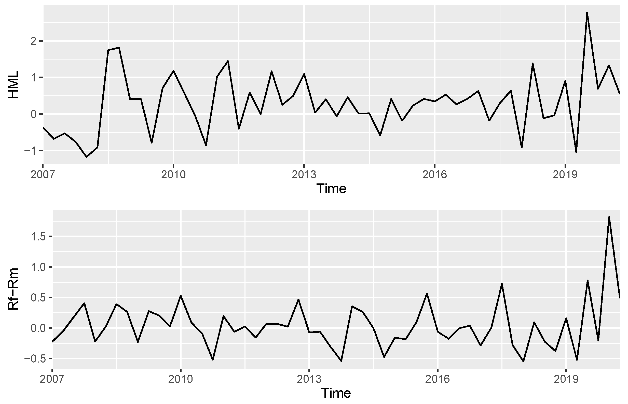
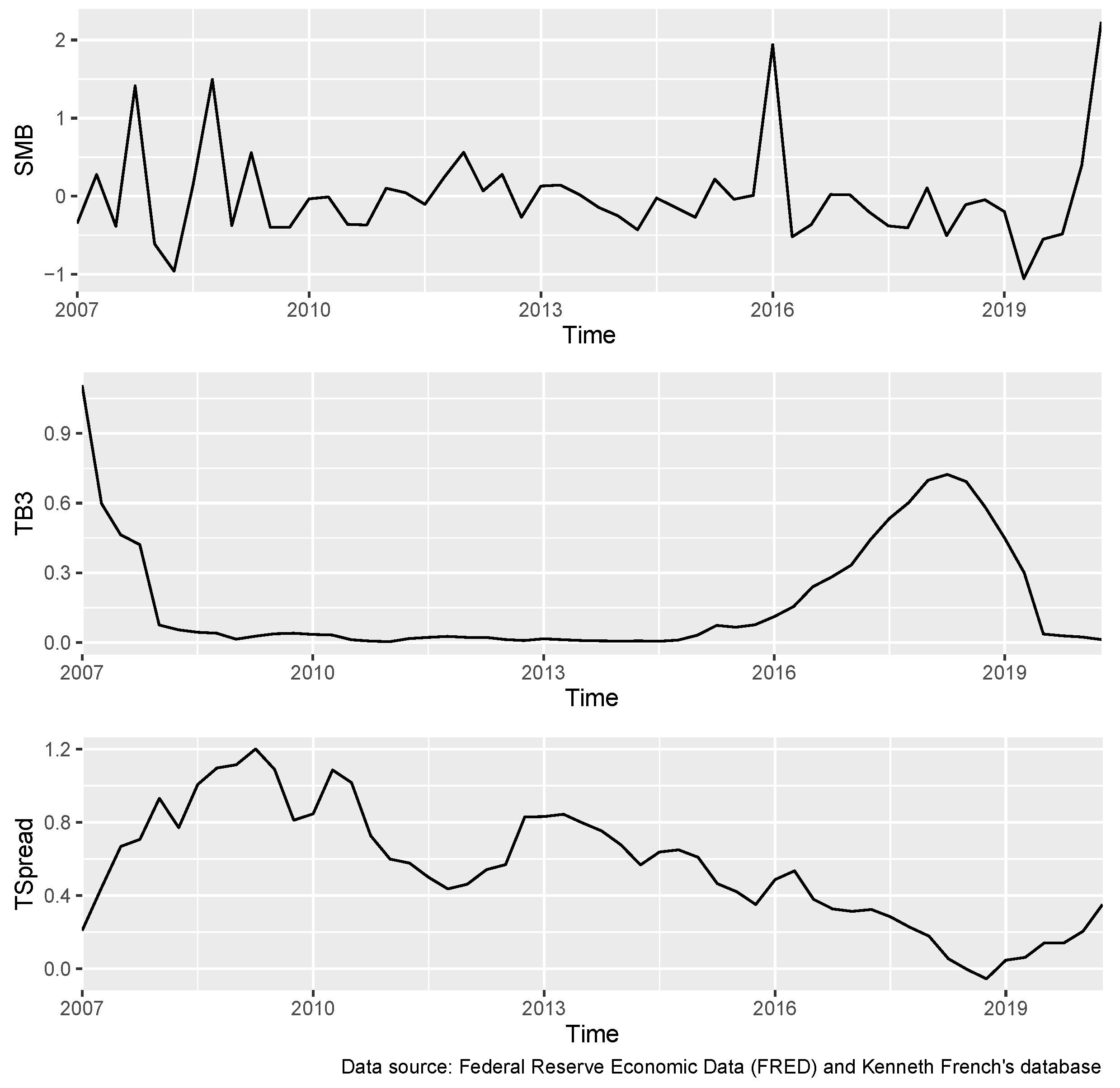
3.3. Macro/Asset-Pricing Variables

As noted in Chan et al. (1990) and Redman and Manakyan (1995), general macroeconomic variables such as inflation (CPI), credit spread (CSpread), and term spread (TSpread) are statistically significant predictors for equity REIT returns. As noted in Fama and French (1993), the market portfolio’s excess return (Rm-Rf), the size factor (SMB), and the value factor (HML) are also statistically significant predictors for equity REIT returns.

Table 2. Correlation Coefficients among Asset Pricing/Macro Control Variables.

	TSpread	TB3	CPI	CSpread	Rm-Rf	SMB	HML
TSpread	1.0000	−0.5878	−0.1170	0.2568	0.0205	0.1052	−0.0288
	(0.0000)	(0.1122)	(0.1377)	(0.1340)	(0.1386)	(0.1379)	(0.1386)
TB3		1.0000	0.2151	−0.1071	−0.1888	−0.1269	−0.2355
		(0.0000)	(0.1354)	(0.1379)	(0.1362)	(0.1376)	(0.1348)
CPI			1.0000	−0.3907	0.0990	0.2058	0.2199
			(0.0000)	(0.1277)	(0.1380)	(0.1357)	(0.1353)
CSpread				1.0000	0.0474	−0.1606	−0.1358
				(0.0000)	(0.1385)	(0.1369)	(0.1374)
Rm−Rf					1.0000	0.2408	0.4792
					(0.0000)	(0.1346)	(0.1217)
SMB						1.0000	0.1747
						(0.0000)	(0.1365)
HML							1.0000
							(0.0000)

Notes: The data from October 2007 to March 2020 on the 3-month U.S. Treasury bill rate (TB3), term spread (TSpread) between 10-Year Treasury bond and 3-month Treasury bill rates, credit spread (CSpread) between Moody’s Seasoned Baa and Aaa corporate bond rates, and inflation (CPI) are retrieved from the Federal Reserve Economic Data (FRED).24 The data during the same period on the Fama-French three factors—the excess return on the market (Rm-Rf), the size factor (SMB), and the value factor (HML)—are retrieved from Kenneth French’s database. 25 The rate of inflation is calculated by taking the log-difference of the Consumer Price Index for All Urban Consumers: All Items in the U.S. City Average (CPIAUCSL) [$log\left(\frac{CPIAUCS{L}_t}{CPIAUCS{L}_{t-1}}\right)=CPI$]. The frequency of the original data is monthly but annualized. Hence, the monthly data need to be divided by 12 (for 12 months) and then converted into the quarterly data [${\prod }_{t=1}^T(1+r_t)-1$] to match the quarterly firm accounting data. The data are expressed in percentage terms. Each cell lists the correlation coefficient estimate and the standard deviation (in the parentheses).

reports that term spread (TSpread) has a moderate negative correlation (−0.5878) with the 3-month Treasury bill rate (TB3). Term spread (TSpread) has a negative but low correlation (−0.1170) with inflation (CPI) but credit spread (CSpread) has a positive but low correlation (0.2568) with term spread (TSpread). Term spread (TSpread) has very low correlations (0.0205, 0.1052, −0.0288) with, respectively, the market portfolio’s excess return (Rm-Rf), the size factor (SMB), and the value factor (HML). Credit spread (CSpread) has low correlations (0.0474, −0.1606, −0.1358) with, respectively, the three stock market factors (Rm-Rf, SMB, and HML) as well. The 3-month Treasury bill rate (TB3) has low negative correlations with all the macro/asset-pricing variables except inflation (CPI). Inflation (CPI) has low negative correlations with the bond market factors (TSpread and CSpread) but has low positive correlations with the stock market factors (Rm-Rf, SMB, and HML). The low correlation (0.1747) between HML and SMB indicates that the value and size factors are orthogonal dimensions of asset pricing. Figure 2 reports the dynamics of these variables. More specifically, the value factor (HML) and the size factor (SMB) declined substantially in 2020. However, the value factor (HML) rebounded quickly and achieved a record-breaking high while the size factor (SMB) climbed back gradually over time. Inflation (CPI) dived hard into the negative territory and reached −3.43% in 2008 while a minor dip was witnessed in 2020. Credit spread (CSpred) rose substantially during the GFC to compensate for the greater uncertainty. Credit spread (CSpread) rose a little during the COVID-19 pandemic.23

3.4. Firm Accounting Variables

The discount rate and expected cash flow are the two main drivers of the present value of a cash-flow-producing asset. The firm’s financial statements provide its historical financial data, based on which investors attempt to estimate the discount rate and expected cash flow. To estimate the discount rate, we need to understand the business and its risks under relevant macro/asset-pricing conditions. To estimate the expected cash flow, we need to understand how historical cash flow was composed and what factors will contribute to the future cash flow. Compared with the numbers in the financial statements in isolation, relative financial ratios derived from the financial statements are more informative when comparing a firm’s performance with reference to the aggregate economy, the firm’s relevant industry, its major competitors within the industry, and its historical performance. There are four main dimensions in ratio analysis: internal liquidity, operating performance, financial risk, and growth (Reilly et al. 2018). Internal liquidity ratios, such as the current ratio (CR) in

Table 3. Glossary and Definitions of Financial Ratios.

Symbol	Variable	Definition and Formula
Basic Series
NS	Net Sales	Revenue − Sale Returns − Allowances − Discounts
CA	Current Assets	Cash and Cash Equivalents + Short-term Investment
	+ Net Receivables + Inventories
SE	Shareholder Equity	Total Assets—Total Liabilities
CL	Current Liabilities	Obligations that are due within the next 12 months
LL	Long-term Liabilities	Obligations that are not due within the next 12 months
DP	Dividend Paid Out	The company’s earnings to distributed to its shareholders
OP	Operating Income	Net Earnings + Interest Expense + Income Taxes
EBITDA	Earning Before Interest, Tax,	Operating Income + Depreciation + Amortization
	Depreciation, and Amortization
IT	Income Tax	Corporate Income Tax
Derived Series
Profitability Ratios
ROA	Return on Asset	$\frac{NetIncome}{TotalAssets}$
ROE	Return on Equity	$\frac{NetIncome}{ShareholderEquity}$
ROI	Return on Investment	$\frac{NetIncome}{AverageInvestedCapital}$
EBITDAMA	EBITDA Margin	$\frac{OperatingIncome\left(EBIT\right)+Depreciation+Amortization}{NetSale}$
Liquidity Ratios
CR	Current Ratio	$\frac{CurrentAssets}{CurrentLiabilities}$
NCATA	Net Current Assets % TA	$\frac{NetCurrentAssets}{TotalAssets}$
Financial Risk
LTDE	LT Debt to Equity Ratio	$\frac{TotalLong-termDebt}{TotalEquity}$
TDE	Total Debt to Equity Ratio	$\frac{TotalDebt}{TotalEquity}$
Asset Management
TAT	Total Asset Turnover	$\frac{NetSales}{AverageTotalNetAssets}$
CET	Cash and Equivalents Turnover	$\frac{NetSales}{CashandEquivalents}$
Per Share
CFPS	Cash Flow per Share	$\frac{NetSales}{AverageTotalNetAssets}$
BVPS	Book Value per Share	$\frac{Fir{m}^{\prime }sCommonEquity}{SharesOutstanding}$

Notes: The quarterly firm accounting variables for all REITs, if available, are retrieved from Mergent Online.

, indicate the ability of the firm to meet its short-term financial obligations by comparing current financial obligations to current assets. Operating performance ratios have two subcategories: operating efficiency ratios and operating profitability ratios. For REITs, it makes more sense to focus on the operating profitability ratios, such as return on assets (ROA) and return on equity (ROE) which show the profits as a percentage of the asset and capital, respectively. The main difference between ROA and ROE is whether the denominator takes into account a company’s debt ($ROE=\frac{NetIncome}{ShareholderEquity}$ and $ROA=\frac{NetIncome}{TotalAssets}$). Risk analysis is concerned with examining the major factors that cause the firm’s cash flow to vary (Reilly et al. 2018). There are two main components: business risk and financial risk. Business risk is defined as the uncertainty due to the firm’s variability of operating earnings caused by its products, customers, and the way it produces its products and services. Financial risk is defined as the additional uncertainty of returns to equity holders due to the firm’s use of debt or bonds (Reilly et al. 2018). When the firm raises capital through borrowing debt or issuing bonds, the interest and principal payments on debt or bonds are fixed contractual obligations. Leverage can enlarge the gain and loss. However, across the boom and bust cycle, the earnings available to shareholders will rise and fall by a wide margin.

The firm accounting data during the period of Q4 2007 Q4—Q3 2021 are retrieved from MergentOnline. The accounting data can be grouped into four main categories: (1) operating performance (ROA, ROE, ROI,26 and EBITDA Margin); (2) internal liquidity (Current Ratio and Net Current Assets/Total Assets); (3) financial risk (Long-term Debt to Equity Ratio and Total Debt To Equity Ratio); and (4) asset management (Total Asset Turnover and Cash and Equivalents Turnover).27

4. Hypotheses, Model, and Estimation and Testing Strategies

4.1. Hypotheses

In the following, we develop four key null and alternative hypotheses ($H1$–$H4$).

It is noted that the COVID-19 pandemic fosters and requires working from home or remote working, movement restrictions, and online shopping, which further boost e-commerce and the demand for industrial REITs’ warehousing and logistics spaces. Therefore, we propose the first null hypothesis that the net impact of the COVID-19 pandemic on industrial REIT returns is zero ($H{1}_0$) against the alternative hypothesis that the net impact is positive ($H{1}_a$).

A favorable attitude shift among U.S. executives and employees towards working from home or remote working is found in a U.S. Remote Work Survey by Price Waterhouse Coopers (PwC) in January 2021.28 In addition, PwC predicts hybrid workplaces where many office employees rotate in and out of becoming more common. Therefore, we propose the second null hypothesis that the net impact of the COVID-19 pandemic on office REIT returns is zero ($H{2}_0$) against the alternative hypothesis that the net impact is negative ($H{2}_a$).

NAREIT reports that the apartment vacancy rates were flat in 2020 but the population moves from urban cores to suburbs due to the safety concern and working from home or remote working. The COVID-19 pandemic has aggravated the affordable housing crisis and millions of Americans face deep rental debt.29 The Emergency Rental Assistance Program was rolled out to help the qualifying households to ease their financial burden. Therefore, we propose the third null hypothesis that the net impact of the COVID-19 pandemic on residential REIT returns is zero ($H{3}_0$) against the alternative hypothesis that the net impact is negative ($H{3}_a$).

There is considerable empirical evidence that retail REITs experienced the greatest price drawdown during the COVID-19 pandemic. In this paper, we attempt to evaluate the net impact of the COVID-19 pandemic on retail REIT returns. Therefore, we propose the fourth null hypothesis that the net impact of COVID-19 on retail REIT returns is zero ($H{4}_0$) against the alternative hypothesis that the net impact is negative ($H{4}_a$).

4.2. Model

To test these hypotheses, we shall propose a reliable model for REIT returns that permit us to retrieve the net impact of the recession induced by the COVID-19 pandemic that is different from that of recessions. The model shall incorporate two dummy variables $BEA{R}_t$ and $COVI{D}_t$ to differentiate the net impact of two more recent recessions in our sample period from that of the most recent recession induced by the Covid-19 pandemic. The model shall incorporate those relevant macro/asset-pricing and firm accounting variables. That is, our generic model is as follows.

$$R_{k,i,t}={\beta }_{k,1}BEA{R}_t+{\beta }_{k,2}COVI{D}_t\times BEA{R}_t+{\beta }_{k,3}Contro{l}_{k,i,t}+{\beta }_{k,4}BEA{R}_t\times Contro{l}_{k,i,t}+{\alpha }_{k,i}+u_{k,i,t}$$

(1)

Here, the first subscript, k, in variables $R_{k,i,t}$, $Contr{l}_{k,i,t}$ and $u_{k,i,t}$ indicates the property type k of REITs. That is, $k=1$ for industrial, $k=2$ for office, $k=3$ for residential, and $k=4$ for retail. Therefore, there are four panel data models with such a model specification, one for each type k. The second subscript, i, in these variables refers to firm i. The third subscript, t, refers to time t. For each panel data model, the slope coefficients ($\beta$’s) in these models are common for all firms (i’s) in the same REIT type k and for all time periods (t’s). The dependent variable, $R_{k,i,t}$, is the excess return on REIT i of property type k at time t (REIT return minus 3-month Treasury bill rate). $Contro{l}_{k,i,t}$ is a vector of control variables for REIT i of property type k at time t, which includes the macro/asset-pricing variables and firm accounting variables. $COVI{D}_t$ is a dummy variable for the most recent recession induced by the COVID-19 pandemic, which equals 1 if t is Q1 2020 and 0 otherwise. $BEA{R}_t$ is a dummy variable for the two recessions covered in the sample of this study, which equals 1 if t belongs to elements in the vector (“Q4 2007”, “Q1 2008”, “Q2 2008”, “Q3 2008”, “Q4 2008”, “Q1 2009”, “Q2 2009”, “Q1 2020”) and 0 otherwise.30 The key coefficient of interest, ${\beta }_{k,2}$, measures the net impact of the COVID-19 pandemic on REITs excess returns of property type k whereas another coefficient of interest, ${\beta }_{k,1}$, measures the net impact of all recessions on REITs excess returns of property type k. When combining these two coefficients, ${\beta }_{k,1}+{\beta }_{k,2}$ measures the aggregate impact of the recession induced by the COVID-19 pandemic. ${\alpha }_{k,i}={\beta }_{k,0}+{\beta }_{k,5}{Z}_{k,i}$ a fixed effect parameter associated with firm i of property type k and it can be viewed as a function of the omitted variables, $Z_{k,i}$, that only vary across firms (i’s) in each property type k but do not change over time (t’s). In each panel data model, the error term for each REIT i of property type k, at time t, $u_{k,i,t}$, is assumed to have a population mean of zero and is uncorrelated with all the independent variables in this model.

4.3. Estimation and Testing Strategies

To select the most reliable model for the excess returns for each type of REIT, five different model specifications are examined.

• In specification 1, the excess returns for each type k of REIT are regressed on all macro/asset-pricing variables and the two dummy variables ($BEA{R}_T$ and $COVI{D}_t$) in the extended Fama–French model to infer the net impacts of the COVID-19 pandemic in particular and that of recessions in general.
• In specification 2, the interaction terms between macro/asset-pricing variables and $BEA{R}_t$ are added to the model in specification 1 to allow structural changes in the macro/asset-pricing variables caused by recessions.
• In specification 3, the firm accounting variables are added to the model in specification 1 to accommodate the impacts of these firm accounting variables.
• In specification 4, the interaction terms between firm accounting variables and $BEA{R}_t$ are added to the model in specification 3 to allow structural changes in these firm accounting variables caused by recessions.
• In specification 5, the interaction terms between macro/asset-pricing variables and $BEA{R}_t$ are added to the model in specification 4 to allow structural changes in both macro/asset-pricing and firm accounting variables caused by recessions.

To explicitly explain the estimation and testing strategies, we suppress property type k and write Equation (1) more compactly using matrix notation.

First, we stack observations across T periods for REIT i of property type k.

$$\underset{T\times 1}{{\mathbf{y}}_{\mathrm{i}}}=\underset{T\times K}{{\mathbf{X}}_{\mathrm{i}}}\mathit{\beta }+{\alpha }_i{\mathit{\iota }}_T+\underset{T\times 1}{{\mathbf{u}}_{\mathrm{i}}},$$

(2)

where $\underset{T\times 1}{{\mathbf{y}}_{\mathrm{i}}}={\left[\begin{array}{c}{y}_{i,1},y_{i,2},\dots ,y_{i,T}\end{array}\right]}^{\prime },$ is the dependent variable vector that contains the excess returns from REIT i of property type k over T periods, $R_{i,1},\dots ,R_{i,T}$;

$$\underset{T\times K}{{\mathbf{X}}_{\mathrm{i}}}=\left[\begin{array}{ccccc}{x}_{i,1}^1& x_{i,1}^2& x_{i,1}^3& \cdots & x_{i,1}^K\\ x_{i,2}^1& x_{i,2}^2& x_{i,2}^3& \cdots & x_{i,2}^K\\ ⋮& ⋮& ⋮& \ddots & ⋮\\ x_{i,T}^1& x_{i,T}^2& x_{i,T}^3& \cdots & x_{i,T}^K\end{array}\right],$$

is the independent variable matrix that contains the dummy variables ($COVI{D}_t$ and $BEA{R}_t$) and control variables for REIT i ($Contro{l}_{i,t}$’s) of property k over T periods; ${\mathit{\iota }}_T$ is a $T\times 1$ vector of unity; $\underset{K\times 1}{\mathit{\beta }}={\left[\begin{array}{c}{\beta }_1,{\beta }_2,\dots ,{\beta }_K\end{array}\right]}^{\prime },$ is the parameter vector of K slope coefficients; ${\alpha }_i$ is the parameter scalar of the fixed effect for REIT i of property k; and, finally, $\underset{T\times 1}{{\mathbf{u}}_{\mathrm{i}}}={\left[\begin{array}{c}{u}_{i,1},u_{i,2},\dots ,u_{i,T}\end{array}\right]}^{\prime }.$ is the vector of error terms for REIT i of property k over T periods.

Second, we stack the above model for all N REITs:

$$\underset{NT\times 1}{\mathbf{y}}=\underset{NT\times K}{\mathbf{X}}\mathit{\beta }+\mathbf{D}\underset{N\times 1}{\mathit{\alpha }}+\underset{NT\times 1}{\mathbf{u}},$$

(3)

where

$$\underset{NT\times N}{\mathbf{D}}={\mathbf{I}}_{\mathrm{N}}\otimes {\mathit{\iota }}_T=\left[\begin{array}{ccccc}1& 0& 0& \cdots & 0\\ 0& 1& 0& \cdots & 0\\ ⋮& ⋮& ⋮& \ddots & ⋮\\ 0& 0& 0& \cdots & 1\end{array}\right]\otimes \left[\begin{array}{c}1\\ 1\\ ⋮\\ 1\end{array}\right],$$

$$\underset{NT\times 1}{\mathbf{y}}=\left[\begin{array}{c}{\mathbf{y}}_1\\ {\mathbf{y}}_2\\ ⋮\\ {\mathbf{y}}_{\mathrm{N}}\end{array}\right],\underset{NT\times K}{\mathbf{X}}=\left[\begin{array}{c}{\mathbf{X}}_1\\ {\mathbf{X}}_2\\ ⋮\\ {\mathbf{X}}_{\mathrm{N}}\end{array}\right],\underset{K\times 1}{\mathit{\beta }}=\left[\begin{array}{c}{\beta }_1\\ {\beta }_2\\ ⋮\\ {\beta }_K\end{array}\right],\underset{N\times 1}{\mathit{\alpha }}=\left[\begin{array}{c}{\alpha }_1\\ {\alpha }_2\\ ⋮\\ {\alpha }_N\end{array}\right],\underset{NT\times 1}{\mathbf{u}}=\left[\begin{array}{c}{\mathbf{u}}_1\\ {\mathbf{u}}_2\\ ⋮\\ {\mathbf{u}}_N\end{array}\right],$$

Third, using the de-meaned approach, we transform all variables from their raw data to deviations from respective mean levels for each REIT and effectively eliminate ${\alpha }_{ki}$ in the resulting de-meaned model.

We use the projection matrices

$$\underset{T\times T}{{\mathbf{Q}}_T}={\mathbf{I}}_T-{\mathit{\iota }}_T{\left({\mathit{\iota }}_T{}^{\mathbf{\prime }}{\mathit{\iota }}_T\right)}^{-1}{\mathit{\iota }}_T^{{}^{\mathbf{\prime }}}=\mathbf{I}-{\mathbf{P}}_T,$$

(4)

$${\mathbf{P}}_T={\mathit{\iota }}_T{\left({\mathit{\iota }}_T^{{}^{\mathbf{\prime }}}{\mathit{\iota }}_T\right)}^{-1}{\mathit{\iota }}_T^{{}^{\mathbf{\prime }}}=T^{-1}{\mathit{\iota }}_T{\mathit{\iota }}_T^{{}^{\mathbf{\prime }}},$$

(5)

to obtain the de-meaned model as

$${\mathbf{Q}}_T{\mathbf{y}}_{\mathrm{i}}={\mathbf{Q}}_T{\mathbf{X}}_{\mathrm{i}}\mathit{\beta }+{\alpha }_i{\mathbf{Q}}_T{\mathit{\iota }}_T+{\mathbf{Q}}_T{\mathbf{u}}_i\Rightarrow {\tilde{\mathbf{y}}}_i={\tilde{\mathbf{X}}}_i\mathit{\beta }+{\tilde{\mathbf{u}}}_i.$$

(6)

More specifically,

$$\left[\begin{array}{c}{\tilde{\mathbf{y}}}_1\\ {\tilde{\mathbf{y}}}_2\\ ⋮\\ {\tilde{\mathbf{y}}}_N\end{array}\right]=\left[\begin{array}{c}{\tilde{\mathbf{X}}}_1\\ {\tilde{\mathbf{X}}}_2\\ ⋮\\ {\tilde{\mathbf{X}}}_N\end{array}\right]\mathit{\beta }+\left[\begin{array}{c}{\tilde{\mathbf{u}}}_1\\ {\tilde{\mathbf{u}}}_2\\ ⋮\\ {\tilde{\mathbf{u}}}_N\end{array}\right],$$

(7)

or

$$\tilde{\mathbf{y}}=\tilde{\mathbf{X}}\mathit{\beta }+\tilde{\mathbf{u}}.$$

(8)

Fourth, the parameter vector of this de-meaned FE model can be estimated by

$${\widehat{\mathit{\beta }}}_{FE}={\left({\tilde{\mathbf{X}}}^T\tilde{\mathbf{X}}\right)}^{-1}{\tilde{\mathbf{X}}}^T\tilde{\mathbf{y}},$$

(9)

and the vector of error terms of this model can be estimated by

$$\widehat{\tilde{\mathbf{u}}}=\tilde{\mathbf{y}}-\tilde{\mathbf{X}}{\widehat{\mathit{\beta }}}_{FE}.$$

(10)

Fifth, the robust standard variance-covariance matrix31 for the parameter vector of ${\mathit{\beta }}_{FE}$ and its estimated counterpart are given, respectively, by

$$Var\left({\widehat{\mathit{\beta }}}_{FE}\right)=Var(\mathit{\beta }+{\left({\tilde{\mathbf{X}}}^T\tilde{\mathbf{X}}\right)}^{-1}{\tilde{\mathbf{X}}}^T\tilde{\mathbf{u}})={\left({\tilde{\mathbf{X}}}^T\tilde{\mathbf{X}}\right)}^{-1}{\tilde{\mathbf{X}}}^{T}E\left(\tilde{\mathbf{u}}{\tilde{\mathbf{u}}}^T\right)\tilde{\mathbf{X}}{\left({\tilde{\mathbf{X}}}^T\tilde{\mathbf{X}}\right)}^{-1}$$

(11)

and

$$\widehat{Var}\left({\widehat{\mathit{\beta }}}_{FE}\right)={\left({\tilde{\mathbf{X}}}^T\tilde{\mathbf{X}}\right)}^{-1}\left(\frac{N}{N-K}\sum _{i=1}^N{\widehat{\tilde{\mathbf{u}}}}_i^2{{\tilde{\mathbf{X}}}_{\mathbf{i}}}^T{\tilde{\mathbf{X}}}_{\mathbf{i}}+\frac{N}{N-K}\sum _{l=1}^m\left(1-\frac{l}{m+1}\right)\sum _{t=l+1}^N{\widehat{\tilde{\mathbf{u}}}}_t{\widehat{\tilde{\mathbf{u}}}}_{t-l}({{\tilde{\mathbf{X}}}_{\mathbf{t}}}^T{\tilde{\mathbf{X}}}_{t-l}+{\tilde{\mathbf{X}}}_{t-l}^T{\tilde{\mathbf{X}}}_t)\right){\left({\tilde{\mathbf{X}}}^T\tilde{\mathbf{X}}\right)}^{-1}.$$

(12)

$\widehat{Var}\left({\widehat{\mathit{\beta }}}_{FE}\right)$ can be calculated by the $vcovNW\left(\right)$ function from R panel data models’ package $\mathbf{plm}$. Hypothesis testing can be implemented in the presence of heteroskedasticity and serial correlation of unknown form after $\widehat{Var}\left({\widehat{\mathit{\beta }}}_{FE}\right)$ is obtained.

Sixth, model selection can be carried out by performing the Wald and F tests for the null hypothesis ${\mathrm{H}}_0$ against the alternative hypothesis ${\mathrm{H}}_a$ in the form of:

$${\mathrm{H}}_0:\mathbf{H}\mathit{\beta }=\mathbf{r}vs{\mathrm{H}}_a:\mathbf{H}\mathit{\beta }\ne \mathbf{r}$$

(13)

where $\mathbf{H}$ is a $q\times K$ matrix of q restrictions, $\mathit{\beta }$ is a $K\times 1$ vector of parameters, and $\mathbf{r}$ is a $q\times 1$ vector of constants. When the null hypothesis ${\mathrm{H}}_0$ is true, the Wald test statistic, $W\left({\widehat{\mathit{\beta }}}_{FE}\right)$, has the asymptotic ${\chi }^2$ distribution with q degrees of freedom and the F test statistic, $F\left({\widehat{\mathit{\beta }}}_{FE}\right)$, has the asymptotic F distribution with q and $NT-N-K$ degrees of freedom:

$$W\left({\widehat{\mathit{\beta }}}_{FE}\right)={(\mathbf{H}{\widehat{\mathit{\beta }}}_{FE}-\mathbf{r})}^T{\left(\mathbf{H}\widehat{Var}\left({\widehat{\mathit{\beta }}}_{FE}\right){\mathbf{H}}^T\right)}^{-1}(\mathbf{H}{\widehat{\mathit{\beta }}}_{FE}-\mathbf{r})=\mathrm{q}F\left({\widehat{\mathit{\beta }}}_{FE}\right)\stackrel{a}{\sim }{\chi }^2\left(q\right)$$

(14)

$$F\left({\widehat{\mathit{\beta }}}_{FE}\right)\stackrel{a}{\sim }F(q,NT-N-K)$$

(15)

5. Empirical Results

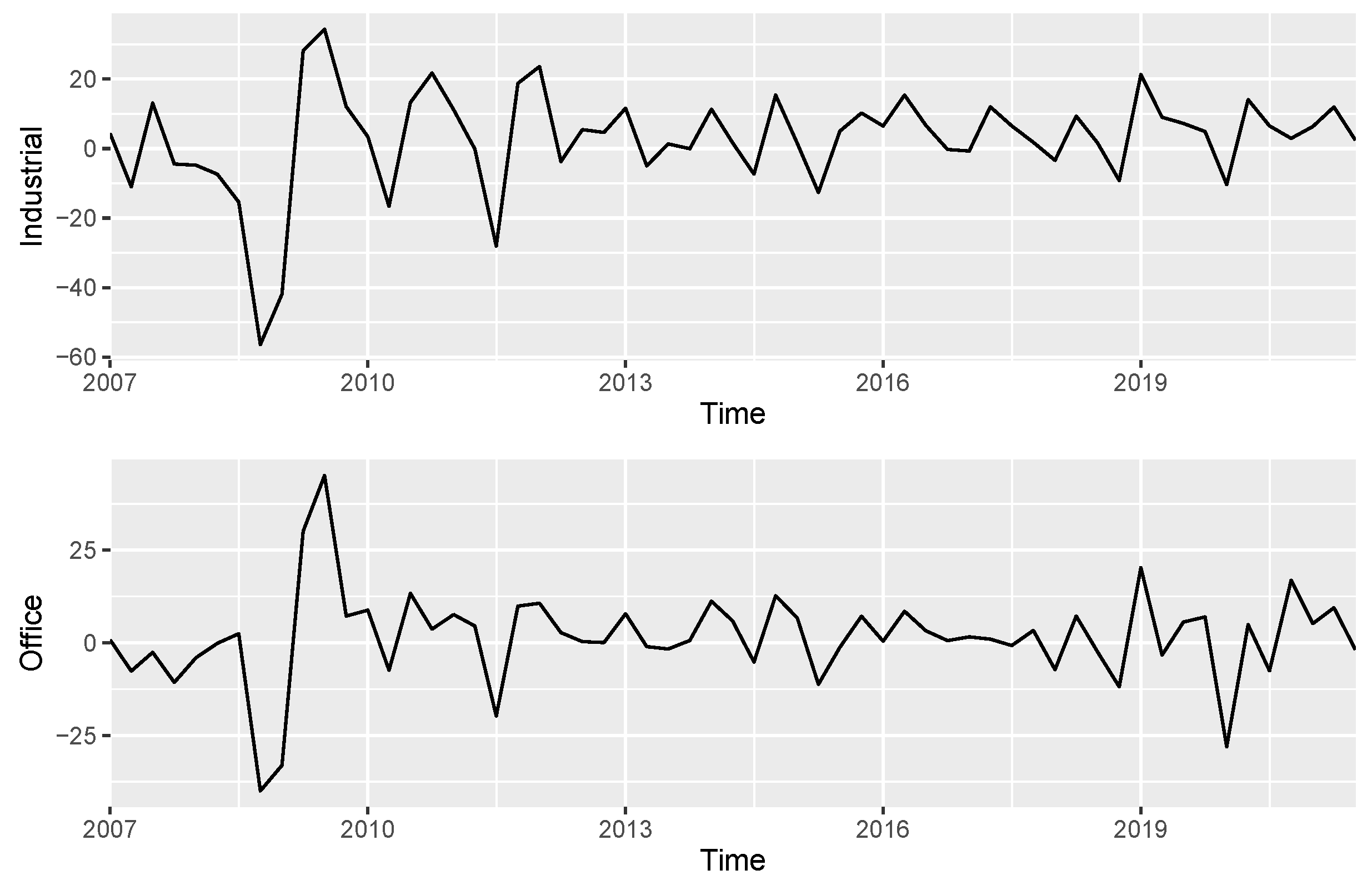
We use the p-values of the F and Wald tests ($F\left({\widehat{\mathit{\beta }}}_{FE}\right)$ and $W\left({\widehat{\mathit{\beta }}}_{FE}\right)$) to compare four pairs of model specifications (1 vs. 2, 1 vs. 3, 3 vs. 4, and 4 vs. 5) for industrial, office, residential, and retail REITs.

Table 4. Model Selection.

Comparison	$\mathit{F}\left({\widehat{\mathit{\beta }}}_{\mathbf{FE}}\right)$	${\mathit{df}}_1$	${\mathit{df}}_2$	p-Value	$\mathit{W}\left({\widehat{\mathit{\beta }}}_{\mathbf{FE}}\right)$	$\mathit{df}$	p-Value
Specification 1 vs. Specification 2
Industrial REITs	147.99	6	378	5.52731 $\times {10}^{-96}$	887.94	6	1.52024 $\times {10}^{-188}$
Office REITs	30.07	6	713	3.17588 $\times {10}^{-32}$	180.42	6	2.76313 $\times {10}^{-36}$
Residential REITs	87.188	6	376	4.01726 $\times {10}^{-68}$	523.13	6	8.73401 $\times {10}^{-110}$
Retail REITs	150.37	6	856	2.95958 $\times {10}^{-201}$	902.19	6	1.26288 $\times {10}^{-191}$
Specification 1 vs. Specification 3
Industrial REITs	2.8861	12	372	0.000792541	34.634	12	0.0005355
Office REITs	1.5226	12	707	0.110737	18.271	12	0.107706
Residential REITs	1.6315	12	391	0.0805092	19.578	12	0.0755018
Retail REITs	0.675	12	850	0.776558	8.0997	12	0.777291
Specification 3 vs. Specification 4
Industrial REITs	2.3618	12	360	0.00620854	28.341	12	0.00493029
Office REITs	2.7998	12	695	0.000952317	33.598	12	0.000780314
Residential REITs	2.4492	12	379	0.00439962	29.39	12	0.00344691
Retail REITs	0.5881	12	838	0.852987	7.0576	12	0.853784
Specification 4 vs. Specification 5
Industrial REITs	36.566	6	354	2.00801 $\times {10}^{-34}$	219.39	6	1.40387 $\times {10}^{-44}$
Office REITs	26.455	6	689	2.06362 $\times {10}^{-28}$	158.73	6	1.09999 $\times {10}^{-31}$
Residential REITs	61.554	6	373	8.00936 $\times {10}^{-53}$	369.32	6	1.09547 $\times {10}^{-76}$
Retail REITs	73.918	6	832	6.81906 $\times {10}^{-74}$	443.51	6	1.22366 $\times {10}^{-92}$

reports the results of these comparisons.

When comparing specification 1 with specification 2, we note that the p-values of both the F and Wald tests for the models for all REITs are substantially less than 0.05. This indicates that the models for all REITs in specification 2 are better supported by the data.

When comparing specification 1 with specification 3, we note that only the p-values of both the F and Wald tests for the model for industrial REITs are substantially less than 0.05 but not for the models for other REITs. This indicates that the model for industrial REITs in specification 3 is better supported by the data while the models for office, residential, and retail REITs in specification 1 are better supported by the data.

When comparing specification 3 with specification 4, we note that the p-values of both the F and Wald tests for the models for industrial, office, and residential REITs are all substantially less than 0.05. However, this is not the case for the model for retail REITs. This indicates that the model for retail REITs in specification 3 is better supported by the data. However, the models for industrial, office, and residential REITs in specification 4 are better supported by the data.

When comparing specification 4 with specification 5, we note that the p-values of both the F and Wald tests for the models for all REITs are all substantially less than 0.05. This indicates that the models for industrial, office, residential, and retail REITs in specification 5 are better supported by the data. We also note that the models in specification 5 are most encompassing among all those in specifications 1–4.

To further analyze these specifications, we report the adjusted $R^2$ (adj. $R^2$’s) of the models for various REITs under these specifications.32 As can be seen in

Table 5. Adj $R^2$’s for Models in Different Specifications.

Specification	Industrial	Office	Residential	Retail
5	0.56	0.54	0.55	0.52
4	0.39	0.47	0.40	0.39
3	0.38	0.44	0.38	0.38
2	0.48	0.46	0.55	0.41
1	0.31	0.38	0.41	0.31

Notes: Adj. $R^2$’s are based on the models for various REITs under various specifications.

, the adj. $R^2$’s for the models for industrial, office, and retail REITs in specification 5 are the highest while the adj. $R^2$’s for the models for residential REITs in specifications 2 and 5 are equally the highest. In other words, while the models for all REITs in specification 5 are supported by the data, the model for residential REITs in specification 2 is as good as that in specification 5. When the analysis of the adj. $R^2$’s is combined with the results from the F and Wald tests, we can reliably select the models for all REITs in specification 5 in our further analysis.

The models in specification 5 incorporate both macro/asset-pricing and firm accounting variables and their respective interaction terms with $BEA{R}_t$. Therefore, these models can accommodate the impacts of all macro/asset-pricing and firm accounting variables, as well as their structural changes during recessions. Using the models in specification 5, we are able to tease out the net impact of $COVI{D}_t$ while controlling the effects of recessions ($BEA{R}_t$), macro/asset-pricing and firm accounting variables, and structural changes during recessions.

Table 6. Model Result—Specification 5.

Variable	Industrial	Office	Residential	Retail
ROA	$0.79$	$0.56$	$0.01$	$0.11$
	$\left(0.46\right)$	$\left(0.25\right)$	$\left(0.26\right)$	$\left(0.33\right)$
ROE	$-0.46$	$-0.14$	$-0.03$	$0.04$
	$\left(0.24\right)$	$\left(0.09\right)$	$\left(0.11\right)$	$\left(0.12\right)$
ROI	$-0.47$	$-0.18$	$0.35$	$0.10$
	$\left(0.43\right)$	$\left(0.18\right)$	$\left(0.52\right)$	$\left(0.26\right)$
EBITDAMA	$0.11$ ***	$-0.02$	$0.03$	$-0.01$
	$\left(0.02\right)$	$\left(0.01\right)$	$\left(0.02\right)$	$\left(0.01\right)$
CR	$-0.14$	$-0.11$	$0.30$	$0.02$
	$\left(0.47\right)$	$\left(0.11\right)$	$\left(0.21\right)$	$\left(0.06\right)$
NCATA	$-0.05$	$0.12$	$-0.08$	$-0.16$
	$\left(0.30\right)$	$\left(0.09\right)$	$\left(0.27\right)$	$\left(0.25\right)$
LTDE	$-11.91$	$-21.76$	$-84.68$	$10.76$
	$\left(15.78\right)$	$\left(13.32\right)$	$\left(44.82\right)$	$\left(30.13\right)$
TDE	$12.02$	$23.87$	$85.21$	$-9.81$
	$\left(15.78\right)$	$\left(13.42\right)$	$\left(44.78\right)$	$\left(30.00\right)$
TAT	$38.78$	$9.42$	$-89.78$ *	$-55.90$
	$\left(45.28\right)$	$\left(34.25\right)$	$\left(41.00\right)$	$\left(36.72\right)$
CET	$0.00$	$0.00$	$0.00$	$-0.00$
	$\left(0.00\right)$	$\left(0.01\right)$	$\left(0.00\right)$	$\left(0.01\right)$
CFPS	$0.04$	$-0.66$	$0.32$	$-0.68$
	$\left(0.52\right)$	$\left(0.30\right)$	$\left(0.39\right)$	$\left(0.53\right)$
BVPS	$-0.05$	$0.09$	$-0.03$	$0.09$
	$\left(0.18\right)$	$\left(0.13\right)$	$\left(0.05\right)$	$\left(0.11\right)$
TSpread	$0.30$	$1.30$	$4.65$ *	$2.65$
	$\left(1.88\right)$	$\left(1.28\right)$	$\left(1.93\right)$	$\left(1.62\right)$
CPI	$-3.84$ *	$-5.93$ ***	$-5.51$ ***	$-6.42$ ***
	$\left(1.46\right)$	$\left(1.01\right)$	$\left(1.06\right)$	$\left(0.98\right)$
CSpread	$41.32$ ***	$26.34$ ***	$32.91$ ***	$50.11$ ***
	$\left(6.30\right)$	$\left(5.81\right)$	$\left(6.80\right)$	$\left(5.54\right)$
Rm-Rf	$4.69$	$3.20$	$1.10$	$3.13$
	$\left(2.03\right)$	$\left(1.33\right)$	$\left(1.47\right)$	$\left(1.27\right)$
SMB	$0.07$	$3.04$ **	$1.25$	$0.43$
	$\left(0.84\right)$	$\left(0.98\right)$	$\left(1.10\right)$	$\left(0.88\right)$
HML	$7.97$ ***	$11.32$ ***	$6.36$ ***	$8.96$ ***
	$\left(1.19\right)$	$\left(0.83\right)$	$\left(0.92\right)$	$\left(0.80\right)$
BEAR	$-75.68$	$-62.30$ *	$-114.70$ ***	$-13.11$
	$\left(38.22\right)$	$\left(26.87\right)$	$\left(35.47\right)$	$\left(31.57\right)$
COVID:BEAR	$46.83$ ***	$22.01$ **	$34.46$ **	$3.88$
	$\left(12.08\right)$	$\left(8.39\right)$	$\left(9.71\right)$	$\left(11.26\right)$
ROA:BEAR	$-8.30$	$-4.51$ *	$-0.22$	$-0.46$
	$\left(4.33\right)$	$\left(2.33\right)$	$\left(1.07\right)$	$\left(1.92\right)$
ROE:BEAR	$2.63$ *	$1.21$	$0.13$	$-0.17$
	$\left(1.40\right)$	$\left(0.77\right)$	$\left(0.31\right)$	$\left(0.49\right)$
ROI:BEAR	$0.39$	$-0.03$	$-1.08$	$0.85$
	$\left(1.39\right)$	$\left(0.74\right)$	$\left(1.14\right)$	$\left(1.09\right)$
EBITDAMA:BEAR	$0.13$	$0.14$ *	$0.01$	$-0.08$
	$\left(0.19\right)$	$\left(0.07\right)$	$\left(0.08\right)$	$\left(0.18\right)$
CR:BEAR	$6.32$	$-2.04$	$1.17$	$0.28$
	$\left(3.46\right)$	$\left(2.06\right)$	$\left(3.20\right)$	$\left(0.38\right)$
NCATA:BEAR	$-3.15$	$0.91$	$0.49$	$-0.81$
	$\left(1.92\right)$	$\left(0.61\right)$	$\left(1.35\right)$	$\left(0.68\right)$
LTDE:BEAR	$48.67$	$-73.42$ **	$-86.24$	$21.26$
	$\left(52.74\right)$	$\left(28.26\right)$	$\left(105.25\right)$	$\left(74.68\right)$
TDE:BEAR	$-56.90$	$60.38$ *	$84.47$	$-22.49$
	$\left(52.80\right)$	$\left(24.95\right)$	$\left(107.14\right)$	$\left(72.91\right)$
TAT:BEAR	$-58.65$	$117.65$ *	$31.55$	$25.42$
	$\left(150.24\right)$	$\left(56.04\right)$	$\left(58.63\right)$	$\left(74.05\right)$
CET:BEAR	$0.00$	$0.11$ **	$-0.00$	$-0.05$
	$\left(0.01\right)$	$\left(0.10\right)$	$\left(0.01\right)$	$\left(0.05\right)$
CFPS:BEAR	$0.32$	$-0.95$	$0.30$	$0.19$
	$\left(1.76\right)$	$\left(1.37\right)$	$\left(1.00\right)$	$0.17$
BVPS:BEAR	$-0.45$	$0.17$	$-0.07$	$-0.03$
	$\left(0.40\right)$	$\left(0.22\right)$	$\left(0.21\right)$	$\left(0.16\right)$
TSpread:BEAR	$193.18$ ***	$118.59$ **	$173.82$ ***	$44.67$
	$\left(58.03\right)$	$\left(35.67\right)$	$\left(52.07\right)$	$\left(42.35\right)$
CPI:BEAR	$26.06$ **	$19.37$ ***	$32.47$ ***	$14.46$ **
	$\left(8.15\right)$	$\left(5.20\right)$	$\left(7.60\right)$	$\left(5.90\right)$
CSpread:BEAR	$-81.95$ ***	$-51.37$ ***	$-24.18$	$-47.13$ **
	$\left(16.71\right)$	$\left(13.75\right)$	$\left(12.68\right)$	$\left(14.39\right)$
Rm-Rf:BEAR	$-202.25$ **	$-110.75$ *	$-211.19$ ***	$-58.42$
	$\left(64.29\right)$	$\left(41.74\right)$	$\left(66.70\right)$	$\left(50.83\right)$
SMB:BEAR	$44.01$ ***	$24.09$ **	$50.86$ ***	28.40 ***
	$\left(11.22\right)$	$\left(7.78\right)$	$\left(11.96\right)$	$\left(8.69\right)$
HML:BEAR	$8.75$ **	$1.38$	$-1.57$	$10.24$ ***
	$\left(6.41\right)$	$\left(4.64\right)$	$\left(2.56\right)$	$\left(4.95\right)$
R${}^2$	$0.61$	$0.57$	$0.60$	$0.55$
Adj. R${}^2$	$0.56$	$0.54$	$0.55$	$0.52$
N	8	15	9	19
T(Unbalanced Panel)	50	47–50	36–50	1–50
Num. obs.	400	742	420	889
F Statistics	$F_{38,49}=49.3597$	$F_{38,49}=19.7187$	$F_{38,49}=54.4208$	$F_{38,49}=24.431$
p-value	2.61132 $\times {10}^{-28}$	3.15609 $\times {10}^{-19}$	2.63781 $\times {10}^{-29}$	2.72225 $\times {10}^{-21}$

*** p < 0.001; ** p < 0.01; * p < 0.05.

reports the models for the excess returns for industrial, office, residential, and retail REITs using the data from October 2007 to March 2020. The control variables include firm accounting variables (shown as ROA, ROE, …, BVPS in the table), macro/asset-pricing variables (shown as TSpread, CPI, …, HML in the table), and their respective interaction terms with the dummy variable for recessions $BEA{R}_t$ (shown as ROA:BEAR, ROE:BEAR, …, TSpread:BEAR, CPI:BEAR, …, HML:BEAR in the table). The key causal variable for the COVID-19 pandemic is the dummy variable $COVI{D}_t$. We test our hypotheses based on the statistical significance levels and signs of the coefficient (${\beta }_{k,2}$) estimates associated with the causal variable $COVI{D}_t$.

It is important to note that the control variables play two basic functions. First, in addition to the “causal” variable $COVI{D}_t$, all control variables represent the necessary conditioning factors that ensure that the error terms of these models are conditionally mean-independent. Second, the significant coefficient estimates indicate information channels linking these control variables to the excess returns on REITs, although the sign and magnitude of each coefficient estimate are not of our primary interest and concern. Our main focus is on the statistical significance levels and signs of the coefficient (${\beta }_{k,2}$) estimates associated with $COVI{D}_t$, which provide insight into our hypotheses.

First, we examine the firm accounting control variables. As can be seen in Table 6, among firm accounting variables, a higher (lower) EBITDA margin (EBITDAMA) leads to higher (lower) excess returns only for industrial REITs. A higher (lower) Total Asset Turnover (TAT) leads to lower (higher) excess returns for residential REITs. For the interaction terms between $BEA{R}_t$ and firm accounting variables, the coefficient estimates associated with the interaction terms between $BEA{R}_t$ and some firm accounting variables such as ROA:BEAR, EBITDAMA:BEAR, LDTD:BEAR, TDE:BEAR, TAT:BEAR, and CET:BEAR are statistically significant only for office REITs indicating these REITs are subject to substantial structural changes in firms’ finance during recessions.

Second, we examine macro/asset-pricing control variables. As can be seen in Table 6, among macro/asset-pricing variables, inflation (CPI) is negatively correlated with excess returns for all REITs. Credit spread (CSpread) is positively associated with excess returns for all REITs. However, when credit risk is higher, REITs would perform better perhaps because REITs invest in more defensive real assets. The size factor (SMB) plays a positive role only for office REITs. The value factor (HML) is significantly positive for all REITs. For the interaction terms between $BEA{R}_t$ and macro/asset-pricing variables, the coefficient estimates associated with TSpread:BEAR, CPI:BEAR, CSspread:BEAR, Rm-Rf:BEAR, SMB:BEAR, and HML:BEAR are all statistically significant. This means that, during recessions, term spread (TSpread), inflation (CPI), and the size factor (SMB) are positively associated with excess returns for all REITs whereas the market index portfolio’s excess return (Rm-Rf) and credit spread (CSpread) are negatively associated with excess returns for all REITs. During recessions, the value factor (HML) is positively associated with excess returns for industrial and retail REITs.

Third, we examine the net impact of the COVID-19 pandemic in comparison with that of recessions. For industrial, office, residential, and retail REITs ($k=1,2,3,4$) the net impact of recessions can be inferred from the coefficient (${\beta }_{k,1}$) estimates associated with $BEA{R}_t$ whereas the net impact of the COVID-19 pandemic can be inferred from the coefficient (${\beta }_{2,k}$) estimates associated with $COVI{D}_t\times BEA{R}_t$.

When we examine the coefficient (${\beta }_{k,1}$) estimates associated with $BEA{R}_t$ for industrial, office, residential, and retail REITs ($k=1,2,3,4$), we note that, in Table 6, all of these estimates for all REITs are negative but only those for office and residential REITs are statistically significant at the level of 5% and 0.1%, respectively. That is, recessions have negative effects on office and residential REITs. Indeed, recessions do slow down businesses and employment and reduce the demand for office and residential spaces. Would the recession induced by the COVID-19 pandemic cause more damage? To answer this question, we examine the coefficient (${\beta }_{2,k}$) estimates associated with $COVI{D}_t\times BEA{R}_t$ for various REITs ($k=1,2,3,4$). We note that, in Table 6, these estimates are positive but only those for industrial, office, and residential REITs are statistically significant at the level of 0.1%, 1%, and 1%, respectively. In other words, the damage caused by the recession induced by the COVID-19 pandemic appears to be less severe than that in general recessions.

To examine this interpretation further, we now discuss our hypothesis testing and empirical findings on the net impact of the COVID-19 pandemic on the excess returns of various REITs when all other control variables are held constant.

• Industrial REITs
  Our first alternative hypothesis is that the net impact of the COVID-19 pandemic on industrial REIT returns is positive ($H{1}_a$). As shown in Table 6, while the net impact of recessions (BEAR) on industrial REIT returns is negative but statistically insignificant, the net impact of the COVID-19 pandemic (COVID) on industrial REIT returns is positive and statistically significant at the level of 1%. This provides strong evidence for rejecting the first null hypothesis ($H{1}_0$) and favoring the first alternative hypothesis ($H{1}_a$).
• Office REITs
  Our second alternative hypothesis that the net impact of the COVID-19 pandemic on office REIT returns is negative ($H{2}_a$). As shown in Table 6, while the net impact of recessions (BEAR) on office REIT returns is negative and statistically significant at the level of 5%, the net impact of the COVID-19 pandemic (COVID) on office REIT returns is positive and statistically significant at the level of 1%. This provides strong evidence against the second null hypothesis ($H{2}_0$) but it does not favor the second alternative hypothesis ($H{2}_a$) either. The net impact of the COVID-19 pandemic offsets that of recessions for office REITs. This is perhaps caused by both existing office leases and the percentage rent clause for commercial properties during the COVID-19 pandemic.
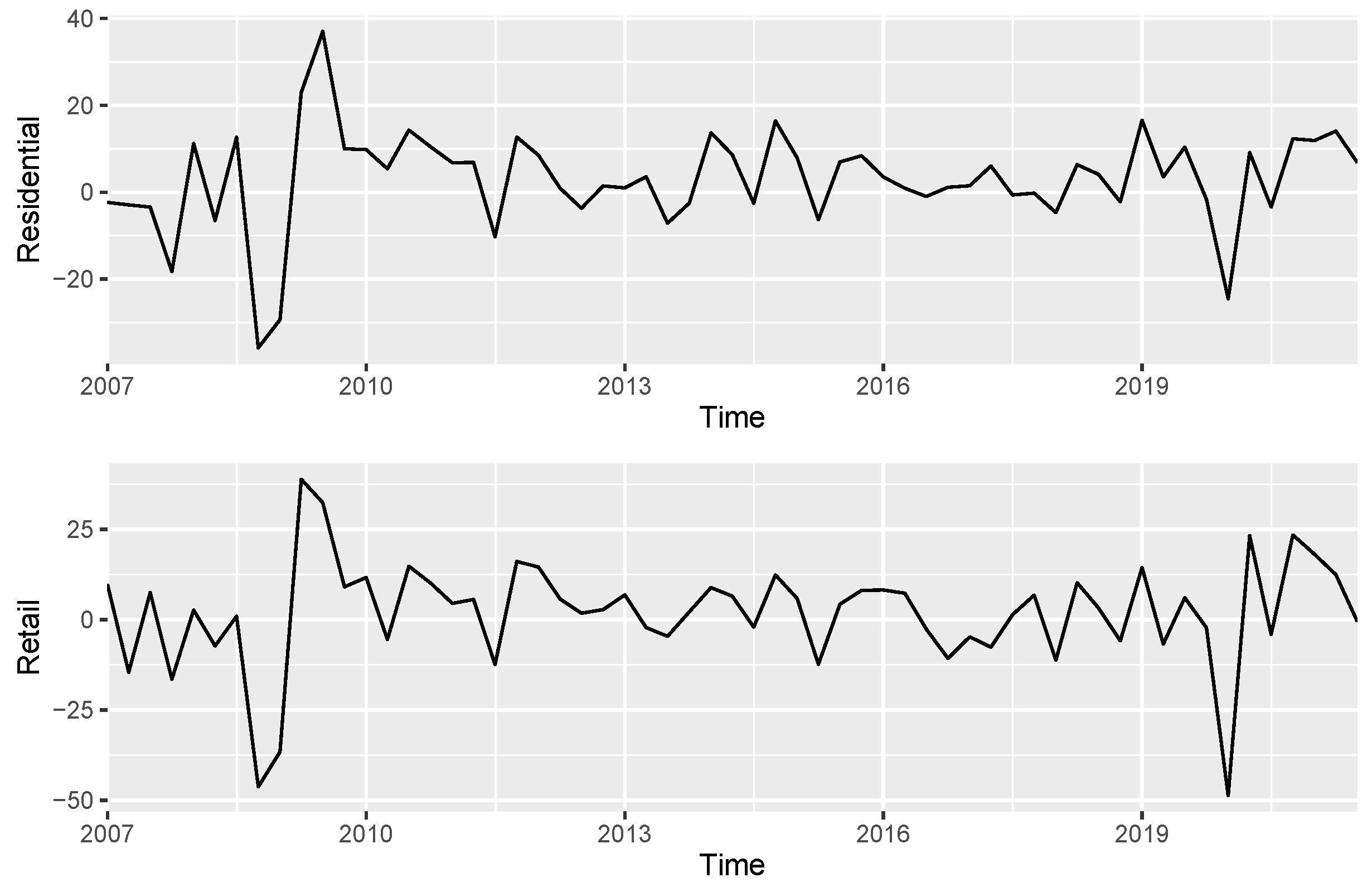
• Residential REITs
  Our third alternative hypothesis is that the net impact of the COVID-19 pandemic on residential REIT returns is negative ($H{3}_a$). As shown in Table 6, while the net impact of recessions (BEAR) on residential REIT returns is negative and statistically significant at the level of 0.1%, the net impact of the COVID-19 pandemic (COVID) on residential REIT returns is positive and statistically significant at the level of 1%. This provides strong evidence against the third null hypothesis ($H{3}_a$) but it does not favor the third alternative hypothesis ($H{3}_a$) either. The net impact of offsets that of recessions for residential REITs. This is perhaps caused by both existing residential leases and the grace period for renting residential properties during the COVID-19 pandemic.
• Retail REITs
  Our fourth alternative hypothesis is that the net impact of COVID-19 on retail REIT returns is negative ($H{4}_a$). As shown in Table 6, while the net impact of recessions (BEAR) on retail REIT returns is negative and statistically insignificant, the net impact of the COVID-19 pandemic (COVID) on residential REIT returns is positive and statistically insignificant. Therefore, we find evidence for the fourth null hypothesis ($H{4}_0$) but against the fourth alternative hypothesis ($H{4}_a$). When all control variables and structural changes are taken into consideration, retail REIT returns are exposed to a long and enduring impact of the boom and bust cycle rather than an isolated impact from recessions.

To infer the aggregate impact of both recessions and the COVID-19 pandemic, we can sum the estimates for parameters ${\beta }_{k,1}$ and ${\beta }_{k,2}$ for REITs of property type k.

For industrial REITs ($k=1$), ${\widehat{\beta }}_{1,1}$ is statistically not significant but ${\widehat{\beta }}_{1,2}$ is statistically significantly different from zero. We can therefore infer ${\widehat{\beta }}_{1,1}+{\widehat{\beta }}_{1,2}=0+46.83>0$, which explains why unconditional industrial REIT returns fell least during the COVID-19 pandemic.

For office REITs ($k=2$), both ${\widehat{\beta }}_{2,1}$ and ${\widehat{\beta }}_{2,2}$ are statistically significant. we can infer ${\widehat{\beta }}_{2,1}+{\widehat{\beta }}_{2,2}=-62.30+22.01<0$, which explains why unconditional office REIT returns fell considerably during the COVID-19 pandemic.

For residential REITs ($k=3$), ${\widehat{\beta }}_{3,1}$ and ${\widehat{\beta }}_{3,2}$ are statistically significant. We can infer ${\widehat{\beta }}_{3,1}+{\widehat{\beta }}_{3,2}=-114.70+34.46<0$, which explains why residential REIT returns also fell considerably during the COVID-19 pandemic.

Finally, for retail REITs ($k=4$), both ${\widehat{\beta }}_{4,1}$ and ${\widehat{\beta }}_{4,2}$ are statistically not significantly different from zero. We can therefore infer ${\widehat{\beta }}_{4,1}+{\widehat{\beta }}_{4,2}=0+0=0$, which suggests that recessions do not shift retail REIT returns. However, Table 6 shows that retail REIT returns maintain strong relations with inflation, credit spread, and the value factor (CPI, CSpread, HML) and structural changes during recessions (CPI:BEAR, CSpread:Bear, SMB:BEAR, HML:BEAR). Therefore, the rise and fall in retail REIT returns closely with ongoing macro/asset-pricing conditions throughout the boom and bust cycle.

6. Conclusions

In this paper, we examine how the net impact of the COVID-19 pandemic differs from that of general recessions using an extended Fama–French model for REIT returns. Differing from the previous recession caused by the GFC, the recession induced by the COVID-19 pandemic caused abrupt and structural changes in economic activity and employment.

Indeed, the COVID-19 pandemic differs from the GFC and it has fostered remote working, restricted people’s mobility, boosted e-commerce, warehousing and logistics, increased unemployment, affected rent affordability, reduced office utilization, and caused business closures. Therefore, we hypothesize that the net impact of the COVID-19 pandemic on industrial REIT returns is positive but the net impacts on office, residential, and retail REIT returns are negative.

To infer the net impact of the COVID-19 pandemic on REIT returns, we must control the impacts of macro/asset-pricing and firm accounting variables and separate the impact cased by recessions from that induced by the COVID-19 pandemic. We use the model selection process to identify the suitable extended Fama–French model for REITs. This model includes the dummy variables for recessions and the COVID-19 pandemic, as well as all macro/asset-pricing and firm accounting variables and their structural changes during recessions. This specification ensures the conditional mean independence of the error term and the proper inference of the net impact of the COVID-19 pandemic.

Using our research methodology, we find that the net impacts of recessions on office and residential REIT returns are negative and statistically significant, but it is not the case for industrial and retail REIT returns. We find that the net impact of the COVID pandemic on industrial REIT returns is indeed positive as anticipated but, contrary to what we anticipated, the net impacts of the COVID-19 pandemic on office and residential REIT returns are not negative. Unexpectedly we find that the net impacts of both recessions and the COVID-19 pandemic on retail REIT returns are statistically insignificant. We also find that, retail REIT returns do not shift by either recessions or the COVID-19 pandemic. The model for retail REIT returns are determined by macro/asset-pricing variables and structural changes throughout the boom and bust cycle, rather than by the shock from either recessions or the COVID-19 pandemic alone.

References

1. Akinsomi, Omokolade. 2021. How resilient are REITs to a pandemic? The Covid-19 effect. Journal of Property Investment & Finance 39: 19–24. [Google Scholar]
2. Alhenawi, Yasser. 2011. The determinants of capital structure in real estate investment trusts. Global Journal of Finance and Economics 8: 119–28. [Google Scholar]
3. Block, Ralph L. 2011. Investing in REITs: Real Estate Investment Trusts. Hoboken: John Wiley & Sons. [Google Scholar]
4. Chan, K. C., Patric H. Hendershott, and Anthony B. Sanders. 1990. Risk and return on real estate: Evidence from equity REITs. Real Estate Economics 18: 431–52. [Google Scholar] [CrossRef]
5. Chen, Nai-Fu, Richard Roll, and Stephen A. Ross. 1986. Economic forces and the stock market. Journal of Business 59: 383–403. [Google Scholar] [CrossRef]
6. Chiang, Kevin C.H. 2015. What drives REIT prices? The time-varying informational content of dividend yields. Journal of Real Estate Research 37: 173–90. [Google Scholar] [CrossRef]
7. Clayton, Jim, and Grey MacKinnon. 2003. The relative importance of stock, bond and real estate factors in explaining REIT returns. Journal of Real Estate Finance and Economics 27: 39–60. [Google Scholar] [CrossRef]
8. Emmerling, Thomas J., Eunkyu Lee, Crocker Herbert Liu, and Yildiray Yildirim. 2022. RETurning to REITs. SSRN. Available online: https://ssrn.com/abstract=4100623 (accessed on 4 May 2022).
9. Fama, Eugene F., and Kenneth R. French. 1992. The cross-section of expected stock returns. Journal of Finance 47: 427–65. [Google Scholar] [CrossRef]
10. Fama, Eugene F., and Kenneth R. French. 1993. Common risk factors in the returns on stocks and bonds. Journal of Financial Economics 33: 3–56. [Google Scholar] [CrossRef]
11. Feng, Zhilan, Chinmoy Ghosh, and C. F. Sirmans. 2007. On the capital structure of real estate investment trusts (REITs). Journal of Real Estate Finance and Economics 34: 81–105. [Google Scholar] [CrossRef]
12. Feng, Zhilan, S. McKay Price, and C. F. Sirmans. 2011. Review articles: An overview of equity real estate investment trusts (REITs): 1993–2009. Journal of Real Estate Literature 19: 307–43. [Google Scholar] [CrossRef]
13. Gyourko, Joseph, and Edward Nelling. 1996. Systematic risk and diversification in the equity REIT market. Real Estate Economics 24: 493–515. [Google Scholar] [CrossRef]
14. Lin, Yu-Cheng, Chyi Lin Lee, and Graeme Newell. 2020. The added-value role of industrial and logistics REITs in the Pacific Rim region. Journal of Property Investment & Finance 38: 597–616. [Google Scholar]
15. Ling, David C., Chongyu Wang, and Tingyu Zhou. 2020. A first look at the impact of COVID-19 on commercial real estate prices: Asset-level evidence. Review of Asset Pricing Studies 10: 669–704. [Google Scholar] [CrossRef]
16. Milcheva, Stanimira. 2022. Volatility and the cross-section of real estate equity returns during Covid-19. Journal of Real Estate Finance and Economics 65: 293–320. [Google Scholar] [CrossRef]
17. Mueller, Glenn. 1995. Understanding real estate’s physical and financial market cycles. Real Estate Finance 12: 47. [Google Scholar]
18. Newey, Whithey K., and Kenneth D. West. 1987. A simple, positive semi-definite, heteroskedasticity and autocorrelation consistent covariance matrix. Econometrica 55: 703–8. [Google Scholar] [CrossRef]
19. Peterson, James D., and Cheng-Ho Hsieh. 1997. Do common risk factors in the returns on stocks and bonds explain returns on REITs? Real Estate Economics 25: 321–45. [Google Scholar] [CrossRef]
20. Redman, Arnold L., and Herman Manakyan. 1995. A multivariate analysis of REIT performance by financial and real asset portfolio characteristics. Journal of Real Estate Finance and Economics 10: 169–75. [Google Scholar] [CrossRef]
21. Reilly, Frank K., Keith C. Brown, and S. Leeds. 2018. Investment Analysis and Portfolio Management. Mason, OH: Cengage. [Google Scholar]
22. Roll, Richard, and Stephen A. Ross. 1995. The arbitrage pricing theory approach to strategic portfolio. Financial Analysts Journal 51: 122. [Google Scholar] [CrossRef]
23. Ross, Stephen A. 1976. The arbitrage theory of capital asset pricing. Journal of Economic Theory 13: 341–60. [Google Scholar] [CrossRef]
24. Schnure, Calvin, Stephanie Krewson-Kelly, Merrie S. Frankel, and Glenn R. Mueller. 2020. Educated REIT Investing. Hoboken: John Wiley & Sons. [Google Scholar]
25. Vincent, Linda. 1999. The information content of funds from operations (FFO) for real estate investment trusts (REITs). Journal of Accounting and Economics 26: 69–104. [Google Scholar] [CrossRef]
26. Wheaton, William C. 1987. The cyclic behavior of the national office market. Real Estate Economics 15: 281–99. [Google Scholar]
Figure 1. Total Return Series of REITs and Market Portfolio Indices.
Jrfm 15 00359 g001
Figure 2. Macro/Asset Pricing Variables.
Jrfm 15 00359 g002