Mitigation Strategies for COVID-19: Lessons from the K-SEIR Model Calibrated to the Observable Data

Abstract

This article develops a detailed epidemiological multi-factor model, the K-susceptible–exposed–infected–removed (K-SEIR) model, and several simpler sub-models as its building blocks. The general model enables us to account for all the relevant COVID-19 features, its disparate impact on different population groups, and interactions within and between the groups. It also includes the availability (or lack thereof) of spare hospital beds and intensive care units (ICU) to accommodate the pent-up demand due to the pandemic. We use the most recent hospitalization and mortality data to calibrate the model. Since our model is multi-factor, we can use it to simulate and analyze the consequences of the sheltering-in-place for each specific group and compare the lives saved and lost due to this measure. We show that in countries with well-developed healthcare systems and a population willing to abide by suitable containment and mitigation procedures, the sheltering in place of the entire community is excessive and harmful when considered holistically. At the same time, sealing nursing homes as thoroughly as possible to avoid high infection and mortality rates is an absolute necessity.

1. Introduction

1.1. Opening Remarks

The first draft of this paper was completed on 5 April 2020 and posted on SSRN on 22 April 2020, Lipton and Lopez de Prado (2020b), while the second iteration was completed on 9 June 2020 and posted on SSRN on 16 June 2020 Lipton and Lopez de Prado (2020c). In the interim, one of us collaborated with D. Gershon and H. Levine and applied the K-SEIR model to study Israel’s situation; see Gershon et al. (2020), posted online on 9 May 2020.

The conclusions at which we arrived at the beginning of the pandemic have stood the test of time and are worth repeating now, when the pandemic has subsided. To this end, below, we present the paper Lipton and Lopez de Prado (2020c) more or less verbatim. When we wrote our paper, the possibility of developing effective vaccines was highly uncertain. Accordingly, we did not discuss vaccination and its benefits in detail. However, our methodology is sufficiently flexible to describe the consequences of vaccination naturally. We added Figure 7, which shows the corresponding flow charts. One section that we felt compelled to add deals with the so-called “Swedish experience”. It discusses the pros and cons of the hands-off approach chosen by the Swedish government to handle the pandemic.

1.2. Pandemics and Their Mitigation

Customarily, pandemics are defined as large-scale outbreaks of infectious diseases that significantly elevate morbidity and mortality over broad geographic areas, if not the whole world, and cause significant disruptions to public health, economics, and politics. Unfortunately, pandemics are common and frequent calamities that have been afflicting humankind since prehistoric times. For instance, the Antonine Plague devastated the Roman Empire in the second century and resulted in a reduction to $2\%$ to $33\%$ of the Roman Empire’s population.The Plague of Justinian killed up to $10\%$ of the population of the Byzantine Empire. In the fourteenth century, the Black Death killed about $30\%$ to $60\%$ of Europe’s population. Closer to our time, due to the unstoppable progress in human mobility, pandemics have continued and even accelerated their malignant progression, despite all the medical advances and breakthroughs. In

Table 1. Recent pandemics and their characteristics. Source: Centres for Disease Control and Prevention (2020).

Name\Params	Period	Place of Origin	Death Toll	Cause
COVID-19	2019–present	China	>0.4 mil	SARS-CoV-2
HIV/AIDS	1981–present	DRC	>36 mil	HIV
The swine flu	2009–2009	Mexico	>0.5 mil	H1N1
The HK flu	1968–1969	HK	>1 mil	H3N2
The Asian flu	1956–1958	China	>2 mil	H2N2
The Spanish flu	1918–1920	Unknown	>20 mil	H1N1
The Russian flu	1889–1890	Turkestan	>1 mil	H3N8 or H2N2
Cholera	1852–1860	India	>1 mil	Vibrio Cholerae

, we briefly summarize some of the pandemics of the last two hundred years, including their most essential characteristics; see Centres for Disease Control and Prevention (2020); Kilbourne (2006).

It is hard to contain and mitigate pandemics when no vaccine or efficient pharmaceutical treatments are available. Therefore, the first to be deployed is the so-called containment strategy to prevent community transmission. Several countries, such as South Korea, Taiwan, and Hong Kong, succeeded in the containment of the initial waves of COVID-19 by using large-scale testing, efficient contact tracing, and timely quarantining of the infected population.1

However, in most countries, including China, Italy, Spain, France, the United Kingdom, and the United States, COVID-19 easily outpaced containment. As a result, these countries had to rely on mitigation strategies to cope with the disease. These strategies were applied with different degrees of vigor and success, resulting in widely varying outcomes. Mitigation strategies relying on nonpharmaceutical interventions are manifold. These strategies include common-sense measures, such as hand hygiene, wearing personal protective equipment, including face masks, travel restrictions, school closures, and social distancing; see, for example, Condon and Sinha (2010); Cowling et al. (2010); Del Valle et al. (2010).

The ultimate mitigation strategy is shelter-in-place, or lockdown, for brevity, which was never used on a large scale before, even during the Spanish Flu of 1918–1919. However, some countries practiced it on a small scale from time to time, usually with minimal success.2 This strategy aims to reduce and delay the peak attack rates and mortality, the so-called “flattening the curve”. However, it is essential to emphasize that flattening the curve is not expected to decrease the total number of cases but rather spread them in time to free the strained capacity of the healthcare system.

In theory, authorities can arrest an epidemic by forcing the majority of the population to shelter in place for a prolonged period while allowing the so-called essential workers to perform their vital duties. In practice, the economic and social price of sheltering-in-place is so high that, after a while, its successful prosecution becomes impossible. The consequences of sheltering in place are dire and easy to fathom since, by its very nature, it is forcing the economies, particularly the service-oriented ones, into a deep recession, if not an outright depression. It causes enormous unemployment, results in incalculable harmful social and health outcomes due to isolation and loneliness, drug abuse, domestic violence, hunger, social unrest, and a partial shutdown of the healthcare system—the very system it is designed to protect.

Leo Tolstoy once said: “Happy families are all alike; every unhappy family is unhappy in its own way”. This observation is equally relevant as far as pandemics are concerned. Several pandemics, including the “Spanish flu” and the “Swine flu”, attacked the so-called low-risk group, comprising the young and healthy, more than the elderly, usually viewed as vulnerable. In sharp and significant contrast, it became clear that COVID-19 attacks the elderly much more aggressively than the young, in line with the common flu and pneumonia. However, age is not the only determinant; the population with pre-existing conditions also belongs to the high-risk group. As a result, the mitigation measures based on sheltering in place of the entire community, rooted in the experience of past pandemics, did not reflect the new reality on the ground.

To evaluate the efficacy of the ultimate mitigation measure—shelter in place—we need to agree on its ultimate purpose. On the one hand, if the ultimate objective of sheltering in place is to buy time until pharmaceutical companies find a vaccine or doctors develop efficient treatments, it can potentially protect people from dying of COVID-19. However, this positive result has to be balanced because prolonged sheltering in place will lead to economic destruction and social meltdown, causing more people to die and suffer from the lockdown than from the disease itself; see Atlas et al. (2020). On the other hand, if the purpose of the shelter-in-place is to slow the spread of pandemics and reduce their peak (flatten the curve), a very different strategy is needed. Flattening the curve is necessary when the healthcare system has limited capacity, especially functional intensive care units (ICUs), and can lead to reduced mortality, even if the total number of infections remains the same over time.

To achieve success, the planner has to clearly and honestly set a goal and develop a strategy accordingly. An understandable desire to be on the safe side is not a viable substitute for actual policy because policymakers have to account for other health issues and the long-term well-being of society.

Early on, several authors, including the present ones, argued that lockdowns are too blunt a tool that will do more harm than good due to the incalculable economic damage, which, in the long run, is tantamount to public health damage, and argued that more subtle approaches must be deployed instead; see Acemoglu et al. (2020); Atlas et al. (2020); Birge et al. (2020); Gershon et al. (2020); Lipton and Lopez de Prado (2020a, 2020b); Shalev-Shwartz and Shashua (2020).

1.3. Epidemiology: Successes and Failures

Given the havoc that epidemics and pandemics play within society, it is only natural to develop a scientific approach to their analysis and possible prevention and mitigation. This approach has to be two-pronged and rooted in medicine and statistics by its very nature. With time, developments in the statistical analysis of various diseases gave birth to epidemiology.

At present, there are four archetypal approaches to epidemiology:

• Susceptible–infected–removed (SIR) and susceptible–infected–susceptible (SIS) models and their extensions, such as susceptible–exposed–infected–removed (SEIR) models;
• Agent-based models;
• Network-based models;
• Simple curve-fitting models that continually attract new enthusiasts despite being largely futile.

There are numerous valuable books covering these approaches; see, for example, Anderson and May (1992); Brauer et al. (2008); Chowell and Hyman (2016); Liu and Stechlinski (2017); Manfredi and D’Onofrio (2013); Martcheva (2015) among others.

In the abstract, the disease is characterized by several parameters, some non-dimensional, some measured in units of time, typically days. The non-dimensional parameters include the basic reproductive number (${\mathfrak{R}}_0$), and various ratios, such as the symptomatic case hospitalization ratio, symptomatic case fatality ratio and others. For example, ${\mathfrak{R}}_0$, an estimate of a pathogen’s transmissibility in a population, is equal to the average number of people that a disease carrier is likely to infect in the absence of any interventions in a population without immunity. The dimensional parameters include the mean number of days from contracting the disease to symptom onset (${\tau }_E$), the mean number of days from symptom onset to hospitalization, recovery, or death (${\tau }_I$), the mean number of days from hospitalization to admittance to the ICU, recovery or deaths (${\tau }_H$), etc.

A disease’s progression can be analyzed top–down using SIR-type models or bottom-up using agent-based models; network-based models are hybrid. Thus, in principle, epidemiologists can build their models ahead of time and use the clinical data about a new disease as they become available in the field to choose the correct values of the relevant parameters and expand or simplify their flow charts appropriately. In 1927, in their seminal paper, Kermack and McKendrick raised mathematical epidemiology to a new level by developing, for the first time, a deterministic epidemic model that included susceptible, infected, and removed individuals; see Kermack and McKendrick (1927).

Epidemiology is very powerful when using SIR-like models for describing certain diseases, primarily occurring in a constrained environment, such as an epidemic of influenza, which happened in a boarding school in the north of England in January and February 1978; see Martcheva (2015). It is much less efficient in dealing with global pandemics. For instance, with regards to modeling COVID-19, it is hard to characterize the hugely influential Imperial College model as an unqualified success; see Ferguson et al. (2020).3 The same is true as far as the Oxford University model is concerned; see Lourenço et al. (2020). The Harvard model, being unimodal, is not particularly well suited for describing COVID-19, which is manifestly multimodal as far as the disease burden is concerned; see Kissler et al. (2020). This fact is particularly puzzling, given that multimodal models for influenza are known; see Choe and Lee (2015).

1.4. Our Methodology

Our primary tool is the K-SEIR model for the K distinct population groups. Using such a model is imperative to adequately capture different responses to the disease by different population groups. Our model broadens the standard SEIR model, a tried and tested working horse of epidemiological studies. However, for studying COVID-19, the SEIR model cannot be used directly for two reasons: (a) The effect of the disease on different population groups is dramatically different; (b) The number of asymptomatic cases is so large that direct evaluation of the so-called basic reproduction number, ${\mathfrak{R}}_0$, is not feasible. To address point (a), we extend the model by introducing the K-SEIR approach. To deal with the second point (b), we propose a novel method where direct calibration of the relevant parameters, such as ${\mathfrak{R}}_0$, is performed by using observable data, including the number of hospitalizations and deaths, rather than the estimated data of the number of infected individuals.

Our methodology is advantageous, compared to the standard methods, which, by construction, cannot handle the particularities of COVID-19. For example, it can assist government bodies in deciding whether to introduce lockdowns and for how long, and which population groups have to be isolated.

1.5. The Structure of This Paper

The paper is organized as follows. In Section 2, we briefly describe the specific characteristics of COVID-19 reported in recent medical publications and summarize the government responses to the pandemic. In Section 3, we consider a homogeneous SEIR model and explain the nature of the relevant parameters. Section 4 presents the all-important discussion of the COVID-19-specific data, such as the number of cases, hospitalizations, and deaths. We also extract useful estimates for the reproductive number and the fatality rates. In Section 5, we introduce the centerpiece of the paper—the K-SEIR model for the K-distinct population groups. In the context of COVID-19, we concern ourselves with two possibilities, namely, the 2-SEIR model, with the two groups being the low-risk (LR) and high-risk (HR), and the 4-SEIR model, with four groups being school children (SC), low-risk (LR), high-risk (HR), and nursing home residents (NH). In Section 6, we extend the K-SEIR model by incorporating the excess mortality into the calculations. We can perform a quantitative comparison of lives saved and lost due to the imposition of lockdowns. In Section 7, we discuss an interesting extension of the K-SEIR model, which replaces derivatives with difference operators and properly accounts for the finite delays in the system. We cover the very important subject of calibration in Section 8.

We base our approach on the assumption that the reproductive number is a latent variable, which we can calculate by matching the hospitalization and mortality data. This matching is an essential expansion of conventional epidemiological approaches, which strive to compute the reproductive number directly. This feature is critical when dealing with COVID-19, as its defining characteristic is a preponderance of asymptomatic or weakly symptomatic cases. This situation is in sharp contrast to, for instance, swine flu, for which each infection was so severe that it led to quarantining and hospitalization. In that case, the direct computation of the reproductive number was relatively straightforward. For COVID-19, the number of reported cases is of tertiary importance unless the authorities undertake massive and continuous testing efforts.

Although not central to our analysis and too simplistic to be of practical value, we start with the archetypal SIR to get an idea of the initial magnitude of the reproductive number before any containment and mitigation measures are implemented. Once our models are calibrated to the data, we use them to analyze the pros and cons of the lockdown strategies in Section 9. We discuss the Swedish experience in Section 10. We briefly discuss our method and its limitations in Section 11. We draw our conclusions in Section 12.

2. COVID-19

2.1. What Is COVID-19?

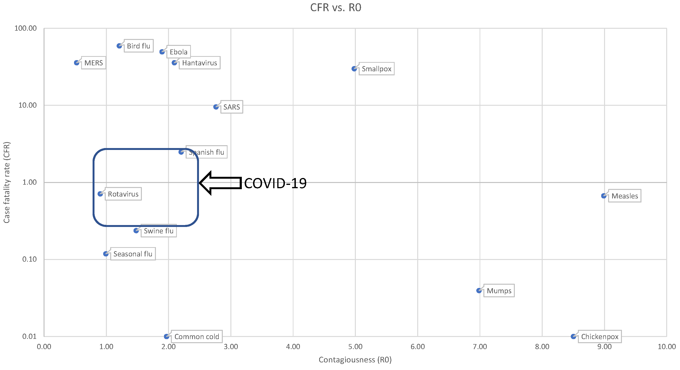
COVID-19 is an infectious disease caused by the severe acute respiratory syndrome coronavirus (SARS-CoV-2). SARS-CoV-2 was first isolated and named on 11 February 2020. The first cases appeared in Huabei (China) in December 2019. As of 6 June 2020, approximately 7 million cases and over 400,000 deaths have been reported across 210 countries; see Worldometers (2020). Transmissibility vs. fatality rates of various diseases, including COVID-19, are summarized in Figure 1.

At present, it is not known whether there is immunity to COVID-19, but most experts think that it is the case.

2.2. Government Responses to COVID-19

On 11 March, the World Health Organization declared COVID-19 a pandemic. Numerous countries have instituted strict controls designed at curbing the spread of the disease, including the following:

• Social distancing for the general population.
• Quarantine (14 days) of individuals returning from infected areas.
• Lockdown/shelter-in-place/stay-at-home of areas with widespread infections.
• Self-isolation of individuals who have tested positive or are suspected to be infected.

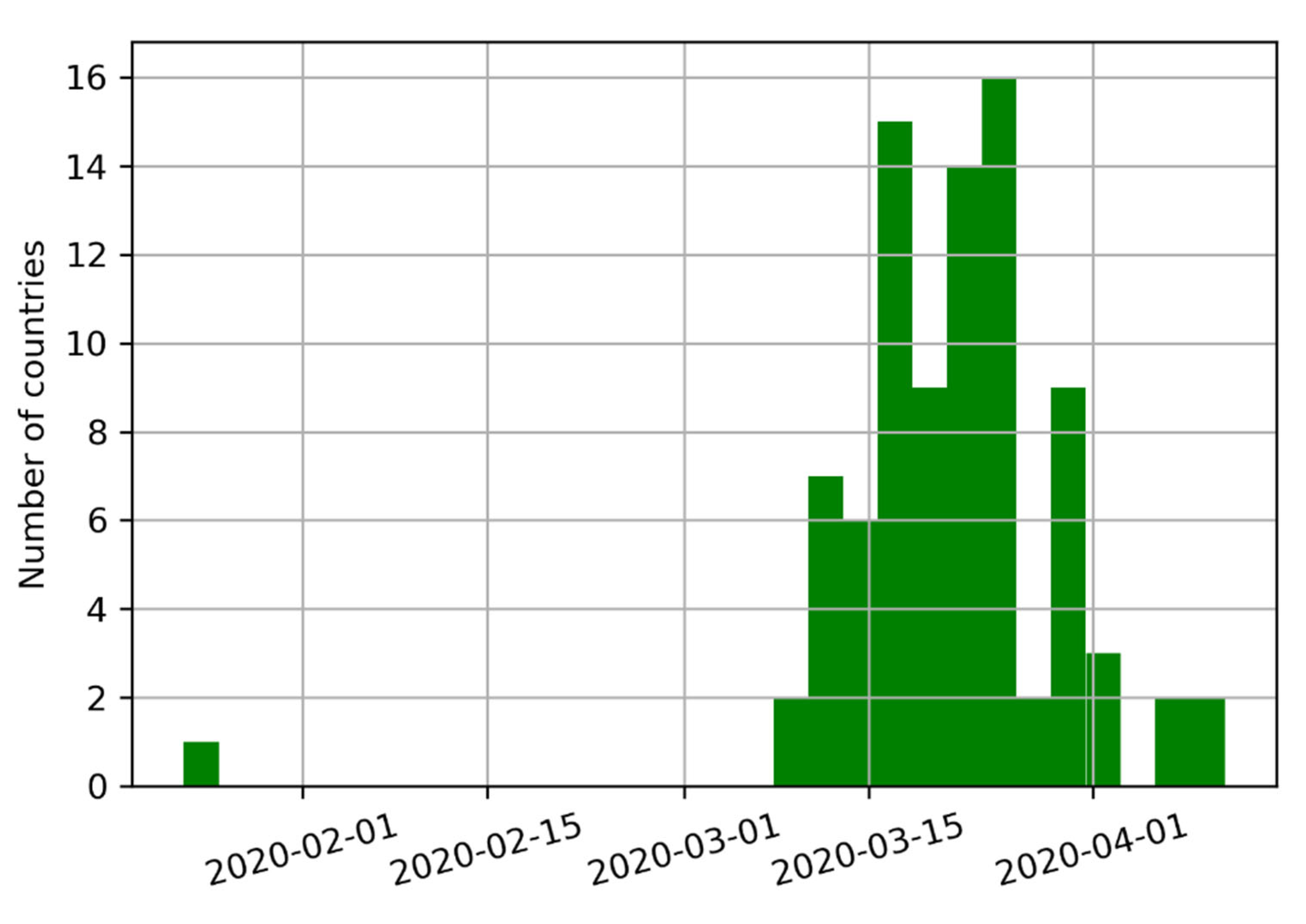
Eighty-eight countries have instituted controls, covering a combined 6.17 billion inhabitants (approx. 79.09% of the World’s population). The median start date for implementing these measures was 22 March 2020. California was the first state in the U.S. to impose a stay-at-home order on 19 March 2020. The deployment of various mitigation measures across the globe is summarized in Figure 2.

2.3. The Great Shutdown

While, first and foremost, COVID-19 is a threat to lives, it is also a threat to livelihoods and, as a result, to more lives. While the virus does not necessarily on its own have a meaningful impact on economic output, government interventions have driven many economies to a halt. In a matter of weeks, the unemployment rate in the United States went from around 3.5% in February 2020 to 19.7% in April 2020, the worst since the Great Depression. At the beginning of the pandemic, economists expected a drop in the U.S. GDP between 8% and 13%. During the Great Recession of 2008–2009, the U.S. GDP fell only by 4.3%.

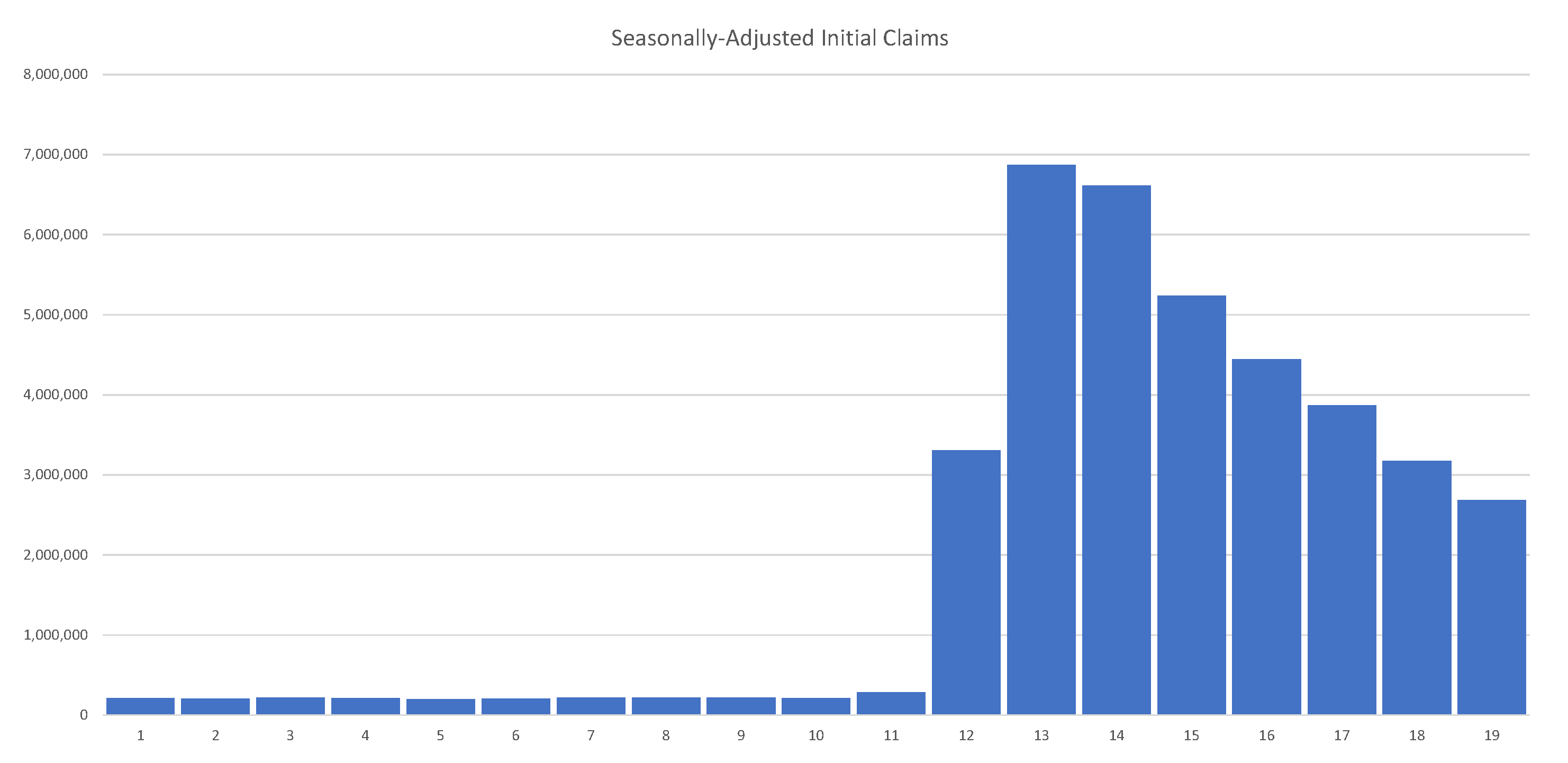
As of 30 May 2020, the U.S. had 40 million unemployed. Job losses over several weeks erased all jobs created over the past decade. Initial unemployment claims in the U.S. are summarized in Figure 3, clearly showing their unprecedented and alarming scale.

Thus, while the pandemic is not an unexpected event by any stretch of the imagination, the government response has been unprecedented.

2.4. The Need for Exit Strategies

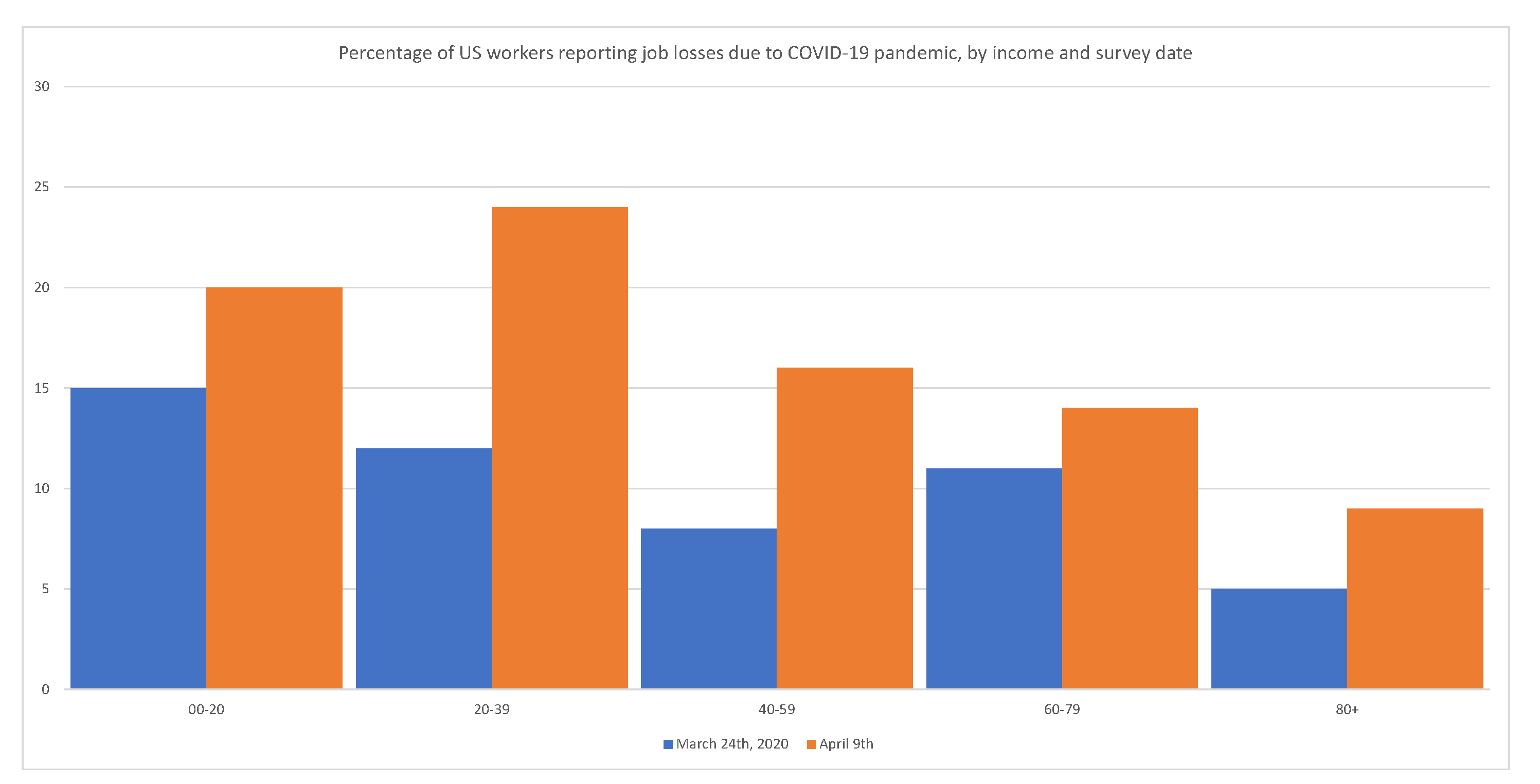
Government interventions have a disproportionately adverse effect on minorities, the working class, and the poor. Figure 4 shows that layoffs have disproportionally affected low-income segments of the population.

Lockdowns will have significant secondary effects for years in terms of health, drug abuse, poor education, family disintegration, etc. For obvious reasons, lockdowns cannot be sustained until a vaccine is available (approx. 18 months). Accordingly, national governments must devise, communicate, and justify their exit strategies.

This study presents a general framework for analyzing the effects of alternative exit strategies.

3. The Standard SIR and SEIR Models

The famous susceptible–infected–removed (SIR) and susceptible–exposed–infected–removed (SEIR) models, originated by Kemrack and McKenrick in 1927, are the main workhorses of mathematical epidemiology. The models are adequate when the entire pool of the susceptible population is well mixed and reacts similarly to the infection.

We start with the SIR model. The corresponding flow chart is shown in Figure 5.

Let S, I, and R, be the number of susceptible, infected, and removed individuals, and N be the total number of individuals alive at time t. The corresponding SIR equations are

$$\begin{array}{ccc}\hfill \frac{dS}{dt}& =& -\frac{{\mathfrak{R}}_0}{{\tau }_I}\frac{I}{N}S,\hfill \\ \hfill \frac{dI}{dt}& =& \frac{{\mathfrak{R}}_0}{{\tau }_I}\frac{I}{N}S-\frac{1}{{\tau }_I}I,\hfill \\ \hfill \frac{dR}{dt}& =& \frac{1}{{\tau }_I}I.\hfill \end{array}$$

(1)

Here, ${\mathfrak{R}}_0$, called the basic reproduction number, is the expected number of secondary cases produced by a single infected individual in a completely susceptible population, absent of any intervention. It can be written in the form

$${\mathfrak{R}}_0=\varkappa \overline{c}{\tau }_I,$$

(2)

where $\varkappa$ is the probability of infection given contact between a susceptible and infected individual (transmissibility), $\overline{c}$ is the average rate of contact between susceptible and infected individuals, and ${\tau }_I$ is the duration of infectiousness. This number is non-dimensional. For the common flu, ${\mathfrak{R}}_0$ is of order 1.2–1.5, but for some highly infectious diseases, it can be as high as 10. We show some representative reproductive numbers in Figure 1 above.

Assuming that N is approximately constant, $N\approx N\left(0\right)$, we can rewrite Equation (1) in relative terms:

$$\begin{array}{ccc}\hfill \frac{ds}{dt}& =& -\frac{{\mathfrak{R}}_0}{{\tau }_I}is,\hfill \\ \hfill \frac{di}{dt}& =& \frac{{\mathfrak{R}}_0}{{\tau }_I}is-\frac{1}{{\tau }_I}i,\hfill \\ \hfill \frac{dr}{dt}& =& \frac{1}{{\tau }_I}i.\hfill \end{array}$$

(3)

An epidemic occurs if

$$di/dt>0⟹{\mathfrak{R}}_{0}is>i.$$

(4)

Since initially $s\approx 1$, an epidemic occurs when ${\mathfrak{R}}_0>1$.

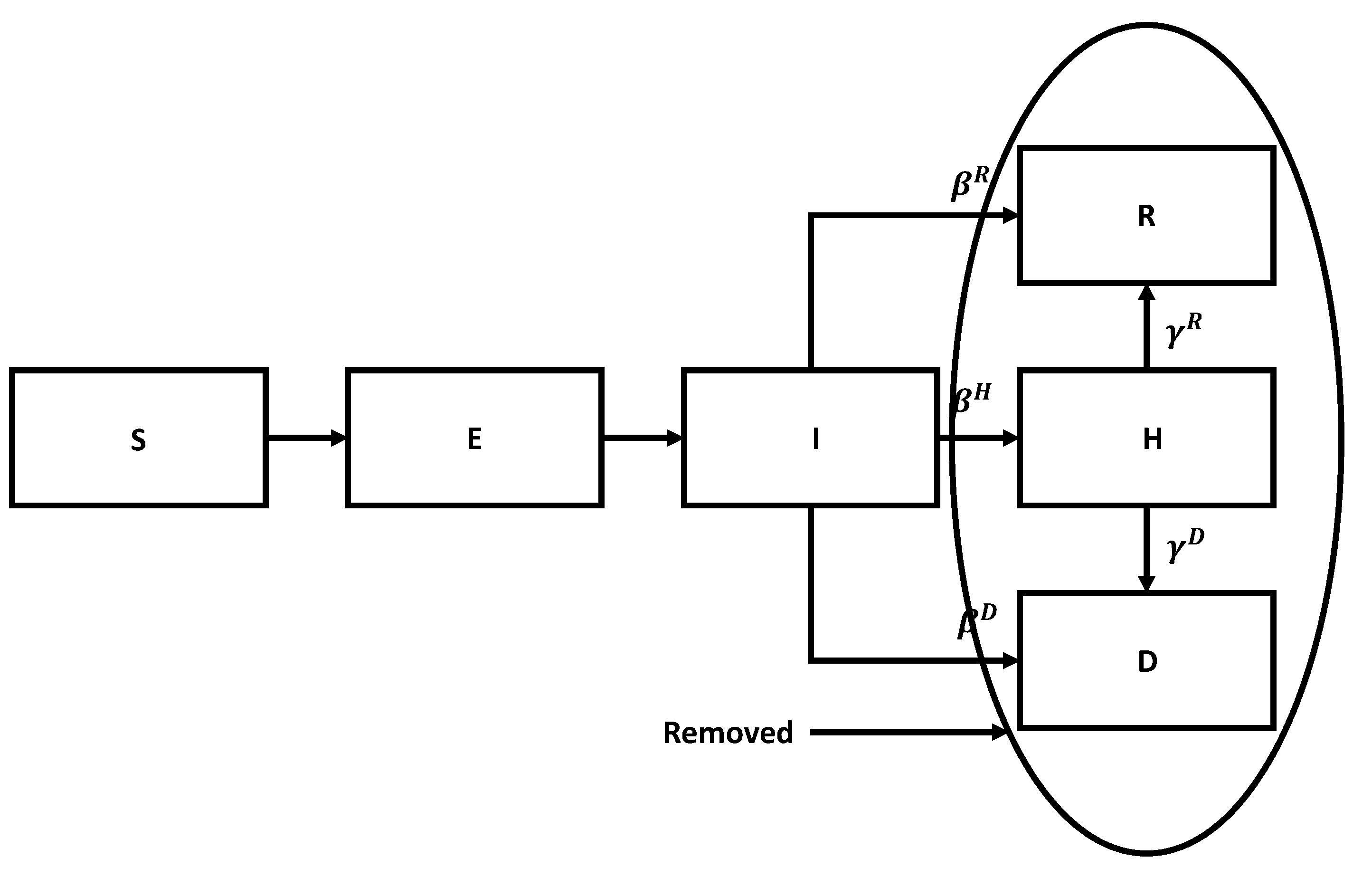
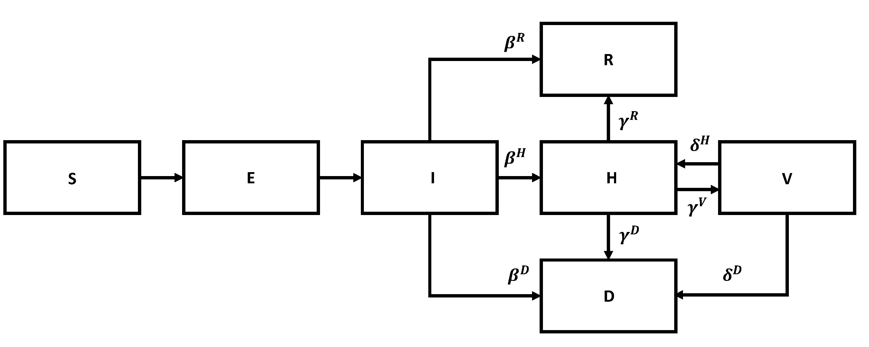
Equations (1) are too simplistic to understand an actual disease in detail. Hence, they need to be generalized as appropriate. Let S, E, I, H, V, R, and D be the number of susceptible, exposed, infected, hospitalized, ICU treated, recovered, and dead individuals, and N be the total number of people at a given moment in time. To adequately describe various stages of the disease, we need to consider several state transitions. The flow chart for the SEIR model is shown in Figure 6.

Susceptible members become exposed upon contact with infected members, exposed become infected after a period, stay infected for a while, and then either recover or die or are admitted to the hospital. Similar stages take place after hospitalization, as per the previous diagram. In a sense, we are dealing with a version of Kirchhoff’s law.

The corresponding governing equations are

$$\begin{array}{ccc}\hfill \frac{dS}{dt}& =& -\frac{\mathfrak{R}}{{\tau }_I}\frac{I}{N}S,\hfill \\ \hfill \frac{dE}{dt}& =& \frac{\mathfrak{R}}{{\tau }_I}\frac{I}{N}S-\frac{1}{{\tau }_E}E,\hfill \\ \hfill \frac{dI}{dt}& =& \frac{1}{{\tau }_E}E-\frac{1}{{\tau }_I}I,\hfill \\ \hfill \frac{dH}{dt}& =& \frac{{\beta }^{\left(H\right)}}{{\tau }_I}I-\frac{1}{{\tau }_H}H+\frac{{\delta }^{\left(H\right)}}{{\tau }_V}V,\hfill \\ \hfill \frac{dV}{dt}& =& \frac{{\gamma }^{\left(V\right)}}{{\tau }_H}H-\frac{1}{{\tau }_V}V,\hfill \\ \hfill \frac{dR}{dt}& =& \frac{{\beta }^{\left(R\right)}}{{\tau }_I}I+\frac{{\gamma }^{\left(R\right)}}{{\tau }_H}H,\hfill \\ \hfill \frac{dD}{dt}& =& \frac{{\beta }^{\left(D\right)}}{{\tau }_I}I+\frac{{\gamma }^{\left(D\right)}}{{\tau }_H}H+\frac{{\delta }^{\left(D\right)}}{{\tau }_V}V,\hfill \\ \hfill \frac{dN}{dt}& =& -\left(\frac{{\beta }^{\left(D\right)}}{{\tau }_I}I+\frac{{\gamma }^{\left(D\right)}}{{\tau }_H}H+\frac{{\delta }^{\left(D\right)}}{{\tau }_V}V\right),\hfill \end{array}$$

(5)

Different phases of the disease are characterized by different characteristic time scales. The corresponding times are denoted by ${\tau }_E$, ${\tau }_I$, ${\tau }_H$, and ${\tau }_V$, respectively. The transition probabilities $\beta ,\gamma ,\delta$ describe the average impact of the disease on the population as a whole. Here,

$$\begin{array}{ccc}\hfill \beta & =& \left({\beta }^{\left(H\right)},{\beta }^{\left(R\right)},{\beta }^{\left(D\right)}\right),{\beta }^{\left(H\right)}+{\beta }^{\left(R\right)}+{\beta }^{\left(D\right)}=1,\hfill \\ \hfill \gamma & =& \left({\gamma }^{\left(H\right)},{\gamma }^{\left(R\right)},{\gamma }^{\left(D\right)}\right),{\gamma }^{\left(H\right)}+{\gamma }^{\left(R\right)}+{\gamma }^{\left(D\right)}=1,\hfill \\ \hfill \delta & =& \left({\delta }^{\left(H\right)},0,{\delta }^{\left(D\right)}\right),{\delta }^{\left(H\right)}+{\delta }^{\left(D\right)}=1.\hfill \end{array}$$

(6)

By construction, Equation (5) satisfies the following conservation laws

$$\begin{array}{ccc}\hfill \frac{d}{dt}\left(S+E+I+H+V+R-N\right)& =& 0,\hfill \\ \hfill \frac{d}{dt}\left(D+N\right)& =& 0,\hfill \end{array}$$

(7)

so that we can drop the equations for R, N, and replace N in the remaining equations by $N\left(0\right)-D\left(t\right)$.

Equation (5) has to be supplied with the initial conditions. We choose these conditions in the form

$$\begin{array}{ccc}\hfill S\left(0\right)& =& \left(1-\xi \right)N_k,E\left(0\right)=\xi N,I\left(0\right)=0,H\left(0\right)=0,\hfill \\ \hfill V\left(0\right)& =& 0,R\left(0\right)=0,D\left(0\right)=0,N\left(0\right)=N,\hfill \end{array}$$

(8)

where N is the initial size of the population in the pool, while $\xi$ is the fraction of the population initially exposed to the virus. In principle, it can be as small as $1/N$—the proverbial “patient zero”. We emphasize that when mixing is not perfect, N can be smaller than the total population in a country or a city.

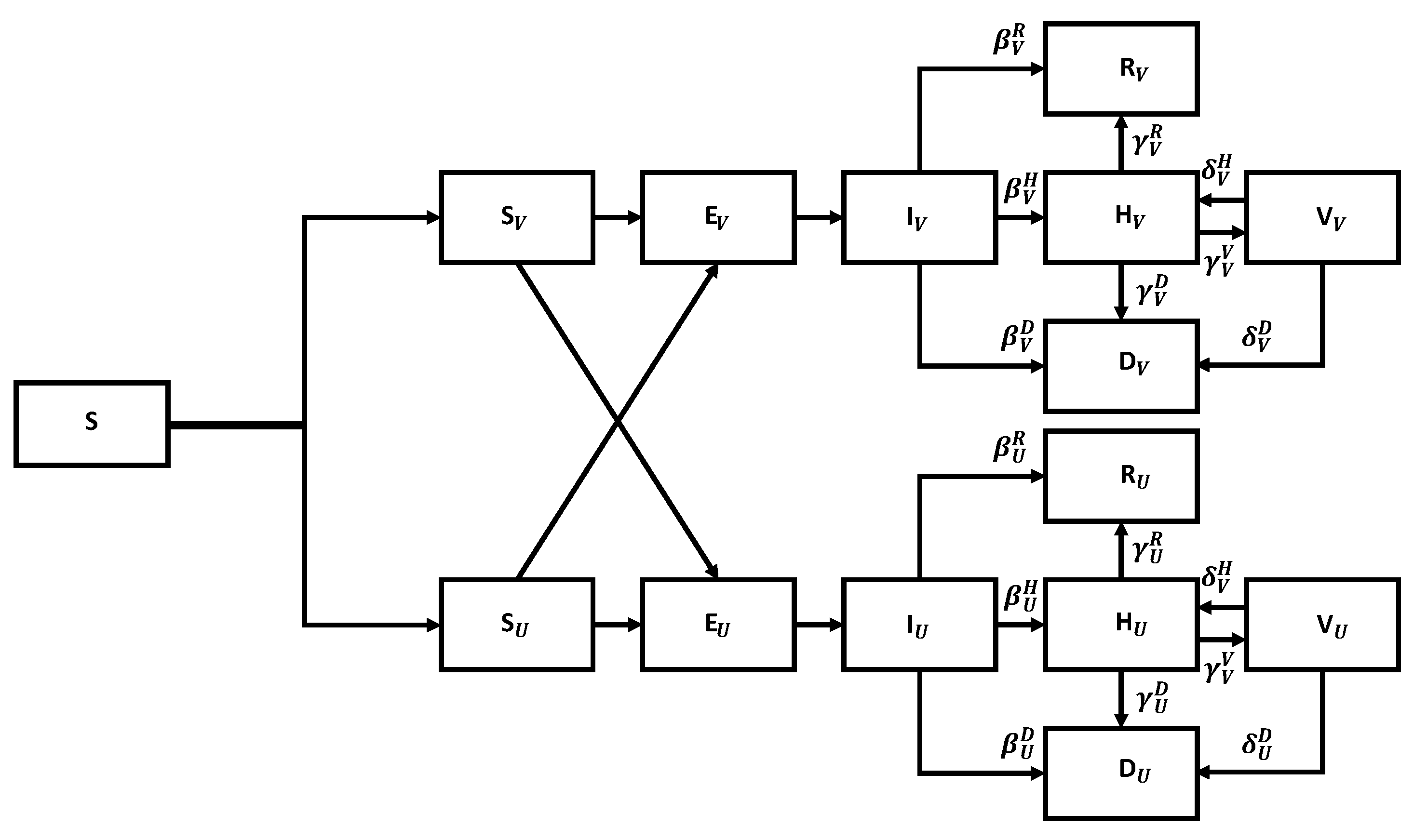
The flow chart for the SEIR model with vaccination is shown in Figure 7.

We can divide susceptible members into vaccinated and unvaccinated classes. Both classes become exposed upon contact with infected members, exposed become infected after a period, stay infected for a while, and then either recover, die, or are admitted to the hospital. The key is that the corresponding parameters are much better for the vaccinated members than for the unvaccinated ones. We leave it to the reader to generalize Equation (5) to describe the corresponding flow chart mathematically.

4. Data and Its Analysis

4.1. Available Data

Time series per country/region is provided by the Johns Hopkins University Center for Systems Science and Engineering (CSSE), which maintains a data repository, with daily counts per country/region of the following variables:

• Confirmed infections (C);
• Deaths (D);
• Recoveries (R).

The number of active cases (A) is implied as A = C − D − R. Additionally, various national agencies report the time series of tests administered (T).

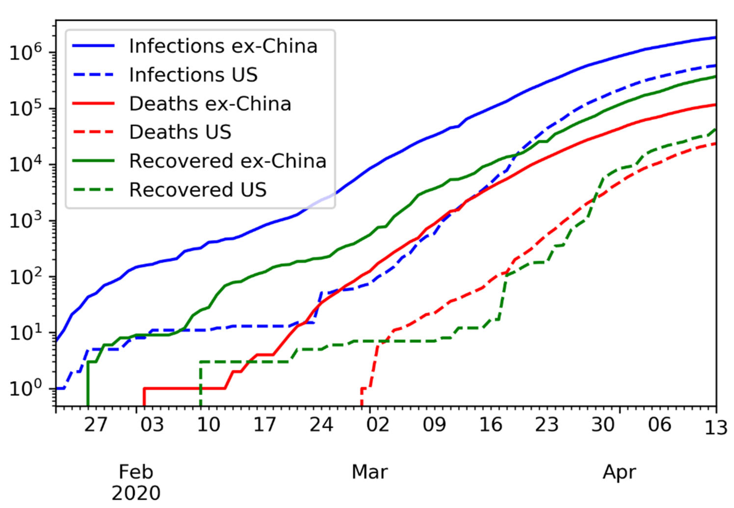
The time series of confirmed infections, deaths, and recovered, in logarithmic scale, is shown in Figure 8.

4.2. Problems with the Data

COVID-19 is a health crisis aggravated by a data crisis. The number of confirmed infections is only a fraction of the number of infections because tested individuals are primarily those where an infection is suspected. The number of tested individuals is lower than the number of tests administered. Individuals, especially essential workers, may require multiple tests to confirm a diagnosis. There is evidence that some countries have manipulated statistics, including China, Indonesia, and Iran. Even after more than 12 weeks since the WHO declared the COVID-19 pandemic, we still do not have accurate statistics; see Figure 9.

Flu pandemics are recurring events. Over the last hundred years or so, they occurred in 1918, 1957, 1968, 2009, and 2020. Because of that, COVID-19 is also a failure of advanced planning.

4.3. Case Fatality Rate

Only a few countries have conducted well-designed statistical experiments to estimate the true values of C, D, R. Given a number of deaths D and a number of recovered individuals R, the maximum likelihood estimate of the case fatality rate d is

$$\widehat{\mathrm{d}}=\frac{\mathrm{D}}{\mathrm{D}+\mathrm{R}}.$$

(9)

That is, $\widehat{\mathrm{d}}$ is the ratio between deaths D and resolved outcomes D + R. This is different from the crude fatality ratio:

$${\widehat{\mathrm{d}}}_{\mathrm{C}}=\frac{\mathrm{D}}{\mathrm{C}}.$$

(10)

The estimate of ${\widehat{\mathrm{d}}}_{\mathrm{C}}$ is less useful because some of the confirmed cases may not resolve favorably.

4.4. Example: The Swine Flu

The Swine Flu pandemic of 2009 was caused by the H1N1 virus; see Table 1. Ten weeks into the epidemic, estimates varied widely between countries, with case fatality rates reported between 0.1% and 5.1%. It took years for doctors to realize that H1N1’s case fatality rate was 0.02%. The problem is that early statistics tends to underestimate the number of recovered individuals R. Flawed data led to a massive overestimation of the fatality rate of H1N1. Eleven years later, data collection is still a challenge; see Figure 10.

It is highly likely that WHO’s original estimate of 3.14% for the COVID-19 case fatality rate is also wrong, for the reasons we establish next.

4.5. Adjusted Fatality Rate for COVID-19

The value of D can be measured with some confidence, because deceased individuals are tracked carefully for legal reasons. In contrast, only a fraction $\theta$ of recovered cases are confirmed, with $\theta \in [0,1]$, due to the over-representation of symptomatic cases in C. Asymptomatic patients are systematically excluded from R. The adjusted fatality rate is

$${\widehat{d}}_{\theta }=\frac{D}{D+{\theta }^{-1}R}\le \widehat{d}.$$

(11)

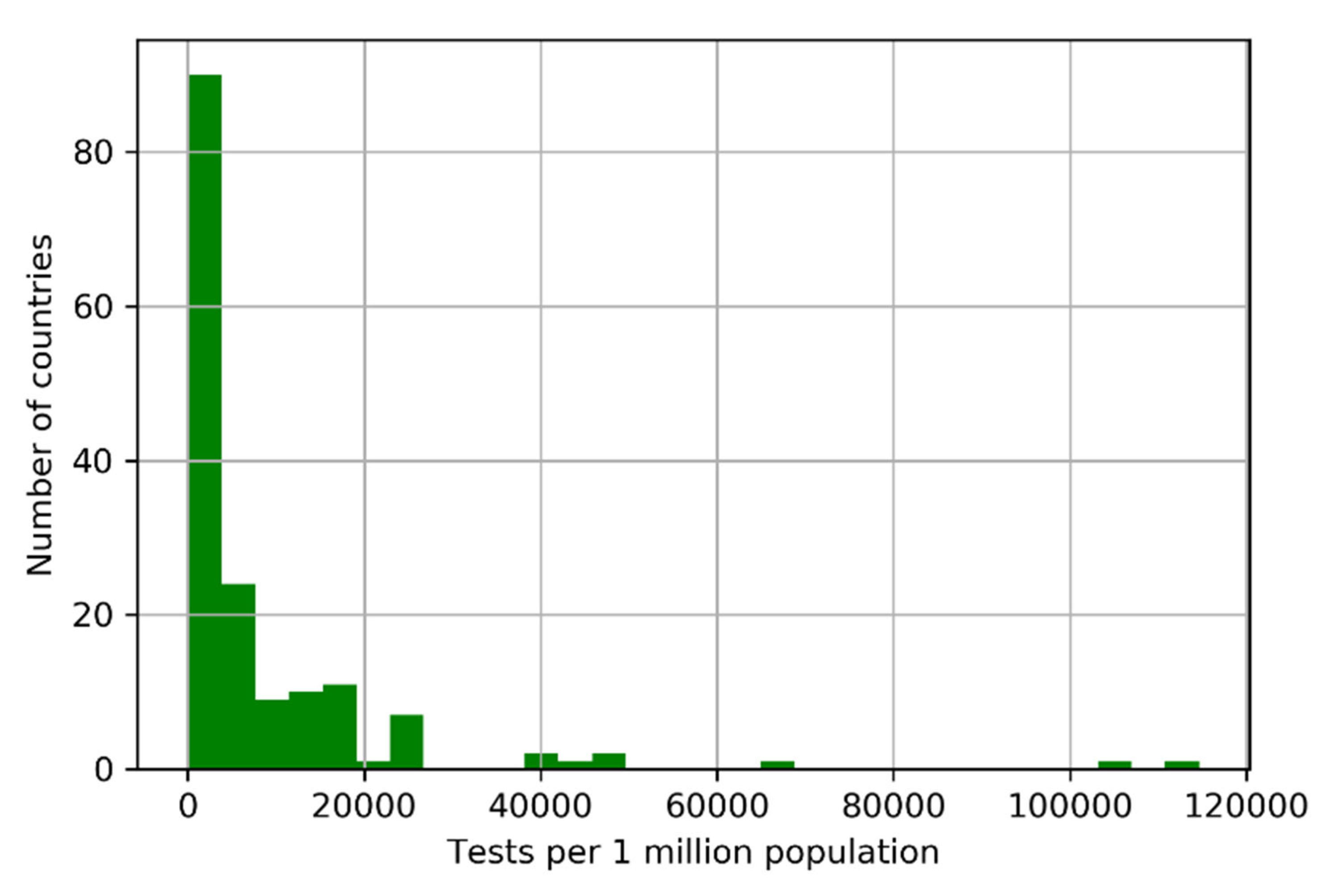
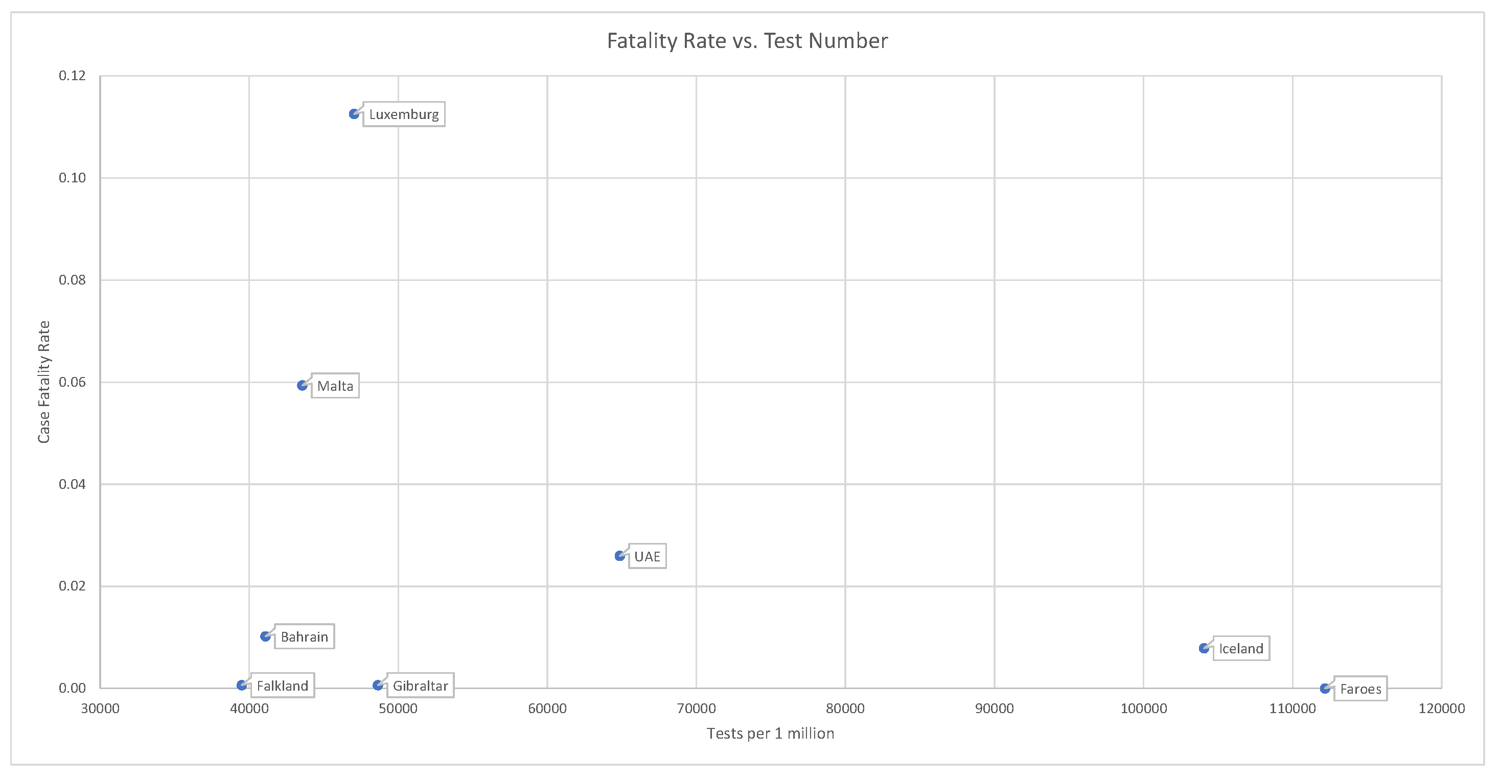
The Chinese CDC estimated that the proportion of mild cases of COVID-19 is approximately 80.9%, thus implying a $\theta <0.191$. Countries that have administered tests to a broader portion of the population tend to report lower case fatality rates; see Figure 11.

This is consistent with the fact that $\theta \ll 1$.

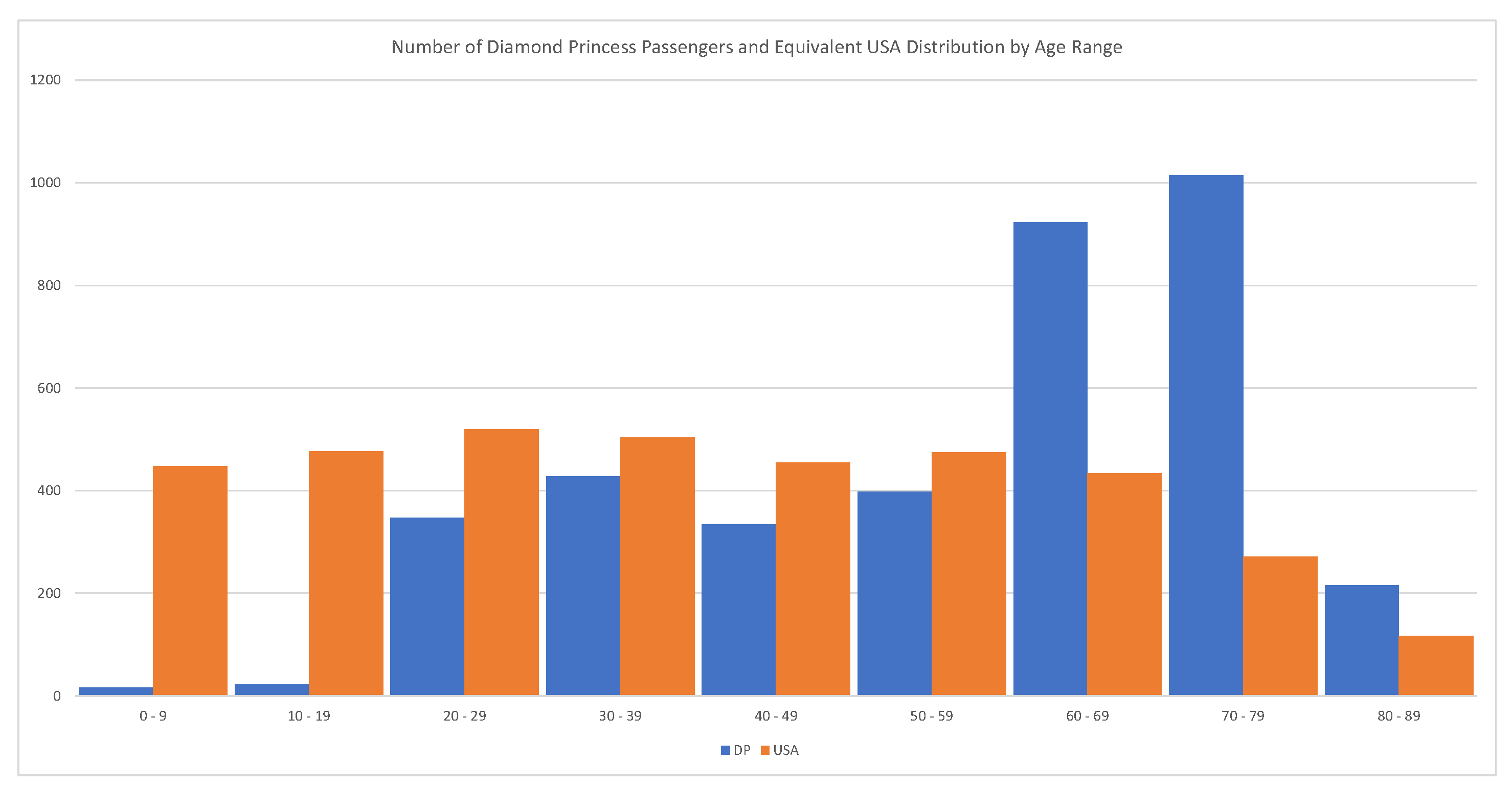
4.5.1. Case Study: The Diamond Princess

Every passenger of the Diamond Princess has been tested ($\theta =1$). In this case, C = 712, D = 12, and R = 644, implying a ${\widehat{d}}_1\approx 1.83\%$; see Russell et al. (2020). The problem with this estimate is that the majority of passengers were between 70–79 years old. We should expect that the global fatality rate for COVID-19 is much lower than 1.83%. The relevant statistics are shown in Figure 12.

4.5.2. Case Study: Iceland

Iceland and the Faeroe Islands are among the countries with most widespread testing relative to their population, and where no new cases are being reported4. So far, the Faeroe Islands has not registered a single death related to COVID-19. At the moment of writing this article, Iceland has administered 62,768 tests on a population of approx. 341,243. Iceland has recorded values of C = 1806, D = 10, and R = 1794.

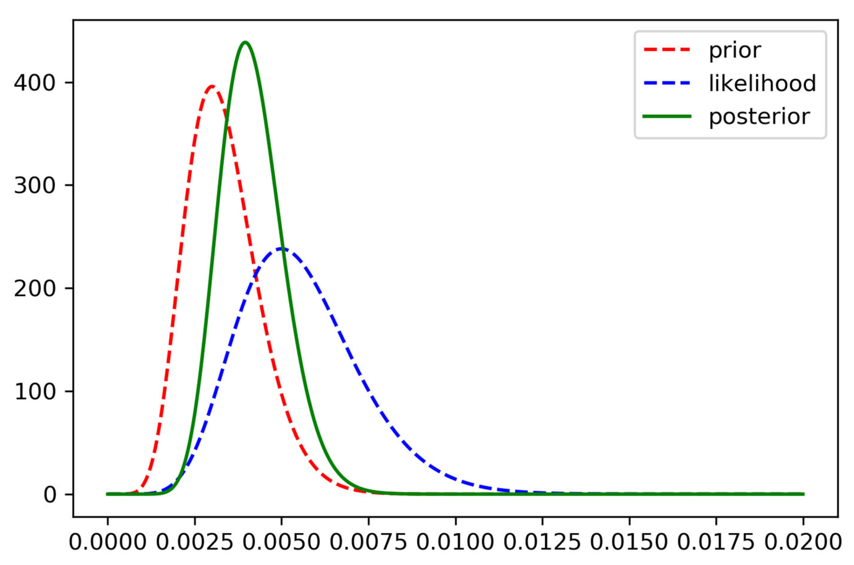
However, even in the case of Iceland, we must accept that $\theta <1$, and $\theta \in [0.191,1]$, since less than 10% of the population has been tested. As a compromise, we use the middle of the range, $\theta =0.6$.

Using a likelihood function $Bi[D+R,{\widehat{d}}_1]$, and a prior $Beta[D,{\theta }^{-1}R]$, we derive a Bayesian estimate of ${\widehat{d}}_{\theta }=0.33\%$ for COVID-19, with $95\%$ confidence bands of $[0.28\%,0.58\%]$; see Figure 13.

This is significantly lower than the WHO’s initial estimate of $3.14\%$.

4.6. Reproductive Numbers and Their Estimation

We must differentiate between the basic and the effective reproductive numbers. The basic reproductive number $\left({\Re }_0\right)$ is the effective reproductive number when there is no immunity from past exposures or vaccination, nor any deliberate intervention in disease transmission.

The effective reproductive number $\left({\Re }_1\right)$ is the number of infections caused by a single individual when some members of the community have developed immunity or some intervention measures are in place.

We can derive the ${\Re }_0$ and ${\Re }_1$ values by fitting the SIR model (3). The value of ${\tau }_I$ can be determined through the direct monitoring of patients, and does not need to be estimated. Given a time series of observations ${\{s_t,i_t,r_t\}}_{(t=1,\dots ,T)}$, we can determine $\widehat{\beta }={\mathfrak{R}}_0/{\tau }_I$ by fitting the equation

$$\Delta i_{t+1}+i_t/{\tau }_I=\beta s_t{i}_t+{\epsilon }_t,$$

(12)

with solution

$$\mathfrak{R}=\frac{{\sum }_{t=1}^T\left(\Delta i_{t+1}+i_t/{\tau }_I\right)s_t{i}_t}{\beta {\sum }_{t=1}^T{\left(s_t{i}_t\right)}^2}.$$

(13)

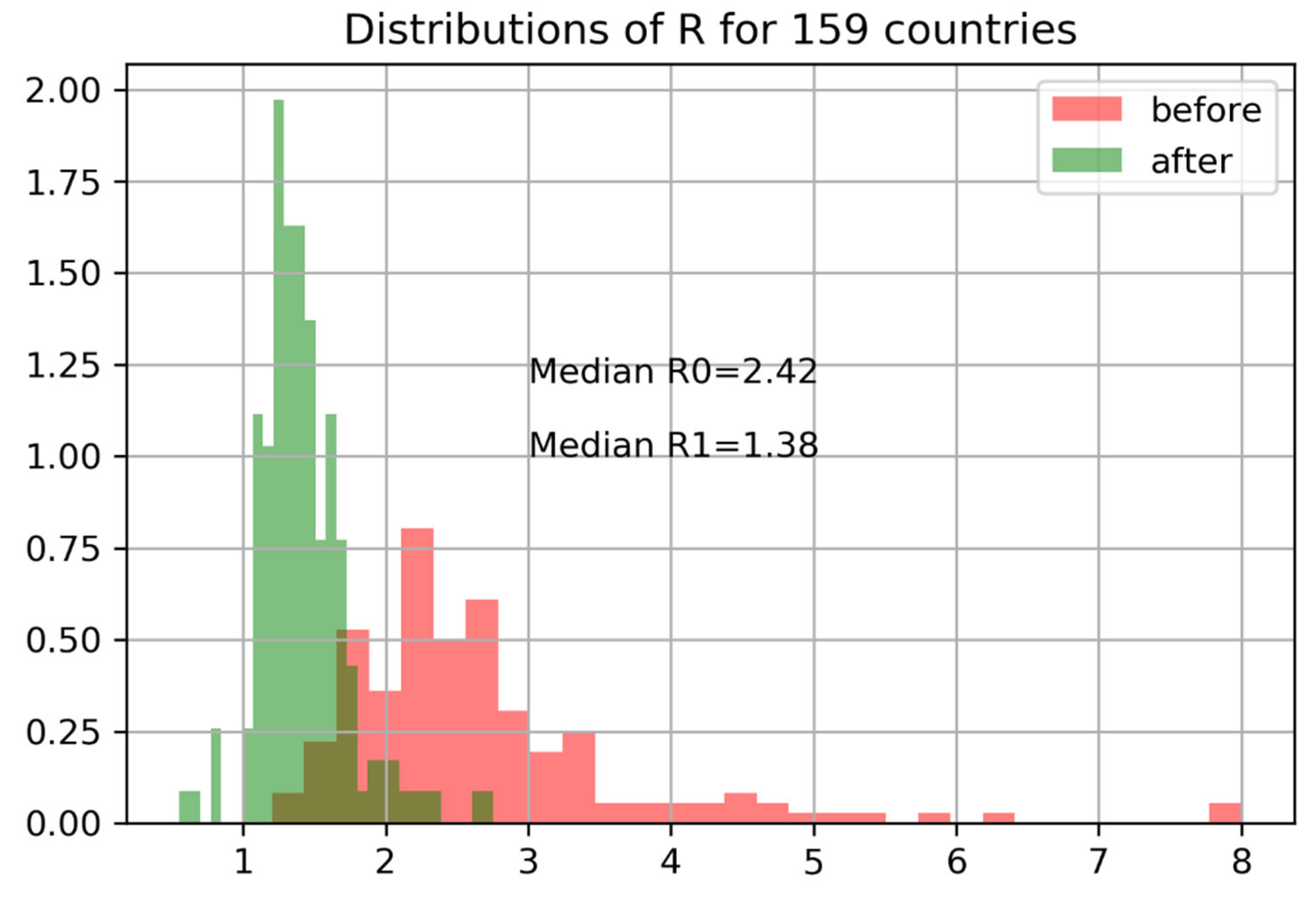
The distribution of ${\Re }_0$ and ${\Re }_1$ across 159 countries shows a steep decline in reproductive numbers following interventions is shown in Figure 14.

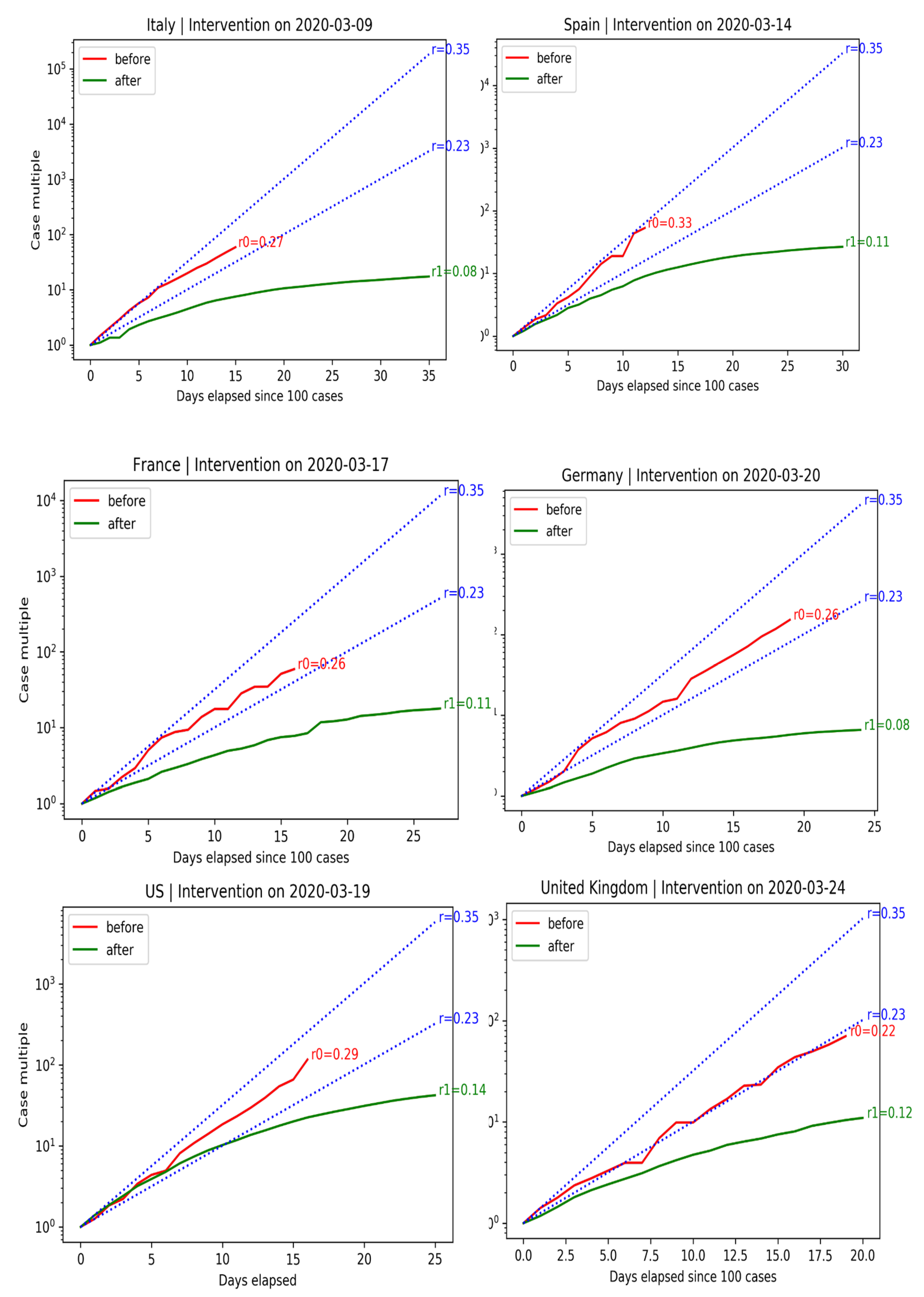
We can evaluate the effectiveness of interventions in terms of confirmed infections before and after measures were adopted. The right plot shows the exponential growth rate in C before and after government intervention. Data before C ≥ 100 are dropped (size is too small of an epidemic). The blue lines indicate expected growth when cases double every two days ($r=0.35$). Cases double every three days ($r=0.23$).

Spain and Italy have economies that rely heavily on tourism. The situation in Spain was particularly alarming, with cases almost doubling every two days. Government-mandated lockdowns successfully curbed the spread of the disease.

France and Germany also experienced exponential growth. Their governments were able to tame the spread of the disease without resorting to drastic lockdowns, like Spain and Italy.

Before the government intervened, cases grew in the U.S. exponentially, at a growth rate of $0.29$. Even after the intervention, it took ten days for cases to fall below the doubling-every-three-days line after the intervention. Benefits are not instantaneous.

The United Kingdom did not declare a National Emergency until 24 March 2020. The initial situation in the U.K. was slightly better than in other European countries. Cases doubled every three days before government intervention. After 18 days, the spread of the disease did not slow down, forcing the U.K. government to ban gatherings of more than two people. After measures were adopted, the spread of the disease slowed down. U.K.’s COVID-19 growth rate of $r=0.12$ is in line with other European countries.

The behavior of the growth rate of COVID-19 before and after government interventions is shown in Figure 15.

4.7. Key COVID-19 Characteristics

In the case of COVID-19, the most recent data suggest the choice for the disease characteristics shown in

Table 2. Constant characteristic parameter values for COVID-19; source Khalili et al. (2020); Kucharski et al. (2020); Li et al. (2020); Linton et al. (2020); Russell et al. (2020); Salje et al. (2020); Verity et al. (2020); Woelfel et al. (2020).

Age	0–49 Years	50–64 Years	≥65 Years
Pre-existing immunity	None	None	None
Percentage of transmission occurring prior to symptom onset	40%	40%	40%
Time from exposure to symptom onset (mean)	~6 days	~6 days	~6 days
Time between symptom onsets in an individual and a second individual infected by the first (mean)	~6 days	~6 days	~6 days
Mean number of days from symptom onset to hospitalization (standard deviation)	6.9 (5.0) days	7.2 (5.3) days	6.2 (5.7) days
Mean number of days of hospitalization without admittance to ICU (standard deviation)	3.9 (3.7) days	4.9 (4.3) days	6.3 (5.1) days
Mean number of days of hospitalization with admittance to ICU (standard deviation)	9.5 (7.2) days	10.5 (7.0) days	10.0 (6.8) days
Percent admitted to ICU among those hospitalized	21.9%	29.2%	26.8%
Percent on ventilators among those in ICU	72.1%	77.6%	75.5%
Mean number of days on ventilators (standard deviation)	5.5 (5.3) days	5.5 (5.3) days	5.5 (5.3) days
Mean number of days from symptom onset to death (standard deviation)	14.9 (7.7) days	15.3 (8.1) days	12.9 (7.6) days

and

Table 3. Variable characteristic parameter values for COVID-19; sourse CDC.

Parameters	Scenario	0–49 Years	50–64 Years	≥65 Years	Overall
$\begin{array}{c}{R}_0\end{array}$	$\begin{array}{c}1\\ 2\\ 3\\ 4\\ 5\end{array}$	$\begin{array}{c}2.0\\ 2.0\\ 3.0\\ 3.0\\ 2.5\end{array}$	$\begin{array}{c}2.0\\ 2.0\\ 3.0\\ 3.0\\ 2.5\end{array}$	$\begin{array}{c}2.0\\ 2.0\\ 3.0\\ 3.0\\ 2.5\end{array}$	$\begin{array}{c}2.0\\ 2.0\\ 3.0\\ 3.0\\ 2.5\end{array}$
$\begin{array}{c}\mathrm{Symptomatic}\mathrm{Case}\\ \mathrm{Fatality}\mathrm{Ratio}\end{array}$	$\begin{array}{c}1\\ 2\\ 3\\ 4\\ 5\end{array}$	$\begin{array}{c}0.02\%\\ 0.02\%\\ 0.10\%\\ 0.10\%\\ 0.05\%\end{array}$	$\begin{array}{c}0.10\%\\ 0.10\%\\ 0.60\%\\ 0.60\%\\ 0.20\%\end{array}$	$\begin{array}{c}0.60\%\\ 0.60\%\\ 3.20\%\\ 3.20\%\\ 1.30\%\end{array}$	$\begin{array}{c}0.20\%\\ 0.20\%\\ 1.00\%\\ 1.00\%\\ 0.40\%\end{array}$
$\begin{array}{c}\mathrm{Symptomatic}\mathrm{Case}\\ \mathrm{Hospitalization}\mathrm{Ratio}\end{array}$	$\begin{array}{c}1\\ 2\\ 3\\ 4\\ 5\end{array}$	$\begin{array}{c}1.30\%\\ 1.30\%\\ 2.60\%\\ 2.60\%\\ 1.70\%\end{array}$	$\begin{array}{c}3.60\%\\ 3.60\%\\ 5.70\%\\ 5.70\%\\ 4.50\%\end{array}$	$\begin{array}{c}5.20\%\\ 5.20\%\\ 10.00\%\\ 10.00\%\\ 7.40\%\end{array}$	$\begin{array}{c}2.80\%\\ 2.80\%\\ 4.10\%\\ 4.10\%\\ 3.40\%\end{array}$
$\begin{array}{c}\mathrm{Percent}\mathrm{of}\mathrm{asymptomatic}\\ \mathrm{infections}\end{array}$	$\begin{array}{c}1\\ 2\\ 3\\ 4\\ 5\end{array}$	$\begin{array}{c}20\%\\ 50\%\\ 20\%\\ 50\%\\ 35\%\end{array}$	$\begin{array}{c}20\%\\ 50\%\\ 20\%\\ 50\%\\ 35\%\end{array}$	$\begin{array}{c}20\%\\ 50\%\\ 20\%\\ 50\%\\ 35\%\end{array}$	$\begin{array}{c}20\%\\ 50\%\\ 20\%\\ 50\%\\ 35\%\end{array}$
$\begin{array}{c}\mathrm{Relative}\mathrm{infectiousness}\mathrm{of}\\ \mathrm{asymptomatic}\mathrm{individuals}\end{array}$	$\begin{array}{c}1\\ 2\\ 3\\ 4\\ 5\end{array}$	$\begin{array}{c}50\%\\ 100\%\\ 50\%\\ 100\%\\ 100\%\end{array}$	$\begin{array}{c}50\%\\ 100\%\\ 50\%\\ 100\%\\ 100\%\end{array}$	$\begin{array}{c}50\%\\ 100\%\\ 50\%\\ 100\%\\ 100\%\end{array}$	$\begin{array}{c}50\%\\ 100\%\\ 50\%\\ 100\%\\ 100\%\end{array}$

; see Centres for Disease Control and Prevention (2020); Khalili et al. (2020).

5. The K-SEIR Model

5.1. K-SEIR—SEIR for Several Interacting Groups

The standard SEIR model is adequate provided that the entire population is affected by the disease evenly. However, COVID-19 impacts different population groups differently. Hence, we must extend the SEIR model so that it takes into account the dynamics of different pools of individuals. To this end, we consider a given city and propose the heterogeneous version of the SEIR model, with K groups: the K-SEIR model.

To account for the different impact of the disease on different groups, we need to split the entire population of a given city into K classes. Let $S_k$, $E_k$, $I_k$, $H_k$, $V_k$, $R_k$, and $D_k$ be the number of susceptible, exposed, infected, hospitalized, ICU treated, recovered, and dead individuals in the $k$-th class, and $N_k$ be the total number of people at a given moment in time. Age is clearly an important determinant of which class an individual belongs to, but other factors, such as pre-existing conditions, must be considered. Clearly, we need to study susceptible, exposed, infected, hospitalized, ICU treated, recovered, and dead subgroups within a class, as well as their interactions with other classes. The flow chart for the SEIR model within a given class is the same as before.

Equations:

$$\begin{array}{ccc}\hfill \frac{d{S}_k}{dt}& =& -\frac{{\mathfrak{R}}_k}{{\tau }_I}{\mathsf{\Theta }}_k{S}_k,\hfill \\ \hfill \frac{d{E}_k}{dt}& =& \frac{{\mathfrak{R}}_k}{{\tau }_I}{\mathsf{\Theta }}_k{S}_k-\frac{1}{{\tau }_E}{E}_k,\hfill \\ \hfill \frac{d{I}_k}{dt}& =& \frac{1}{{\tau }_E}{E}_k-\frac{1}{{\tau }_I}{I}_k,\hfill \\ \hfill \frac{d{H}_k}{dt}& =& \frac{{\beta }_k^{\left(H\right)}}{{\tau }_I}{I}_k-\frac{1}{{\tau }_H}{H}_k+\frac{{\delta }_k^{\left(H\right)}}{{\tau }_V}{V}_k,\hfill \\ \hfill \frac{d{V}_k}{dt}& =& \frac{{\gamma }_k^{\left(V\right)}}{{\tau }_H}{H}_k-\frac{1}{{\tau }_V}{V}_k,\hfill \\ \hfill \frac{d{R}_k}{dt}& =& \frac{{\beta }_k^{\left(R\right)}}{{\tau }_I}{I}_k+\frac{{\gamma }_k^{\left(R\right)}}{{\tau }_H}{H}_k,\hfill \\ \hfill \frac{d{D}_k}{dt}& =& \frac{{\beta }_k^{\left(D\right)}}{{\tau }_I}{I}_k+\frac{{\gamma }_k^{\left(D\right)}}{{\tau }_H}{H}_k+\frac{{\delta }_k^{\left(D\right)}}{{\tau }_V}{V}_k,\hfill \\ \hfill \frac{d{N}_k}{dt}& =& -\left(\frac{{\beta }_k^{\left(D\right)}}{{\tau }_I}{I}_k+\frac{{\gamma }_k^{\left(D\right)}}{{\tau }_H}{H}_k+\frac{{\delta }_k^{\left(D\right)}}{{\tau }_V}{V}_k\right),\hfill \end{array}$$

(14)

The actual split of ${\beta }_k,{\gamma }_k,{\delta }_k$ for different classes is somewhat nuanced. It can be inferred from the clinical information.

5.2. Contacts between Groups

In order to describe contacts between groups, we need to introduce the so-called preferred mixing matrix C. We assume that the number of contacts between members of the k-th and $k^{\prime }$-th group, per unit of time is given by

$$\begin{array}{ccc}\hfill C_{k{k}^{\prime }}& =& \left({\pi }_k{\delta }_{k{k}^{\prime }}+\left(1-{\pi }_k\right)\frac{\left(1-{\pi }_{k^{\prime }}\right)a_{k^{\prime }}{N}_{k^{\prime }}}{{\sum }_{\overline{k}=1}^K\left(1-{\pi }_{\overline{k}}\right)a_{\overline{k}}{N}_{\overline{k}}}\right)a_k{N}_k\hfill \\ & =& \left({\pi }_k{\delta }_{k{k}^{\prime }}+\left(1-{\pi }_k\right)\frac{a_{k^{\prime }}{\tilde{N}}_{k^{\prime }}}{{\sum }_{\overline{k}=1}^K{a}_{\overline{k}}{\tilde{N}}_{\overline{k}}}\right)a_k{N}_k,\hfill \end{array}$$

(15)

where ${\delta }_{k{k}^{\prime }}$ is the Kronecker delta, and ${\tilde{N}}_k=\left(1-{\pi }_k\right)N_k$. Here, $\pi =\left({\pi }_1,...,{\pi }_K\right)$, $0\le {\pi }_k\le 1$, is a vector, which characterizes the relative size of interactions within and outside of the k-th group. Our choice of matrix C allows us to consider all kind of possibilities, including the limiting cases when there is proportional mixing between groups (the matrix is degenerate, has rank one, and ${\pi }_k=0$), or there is no mixing between groups at all (the matrix is diagonal, and ${\pi }_k=1$).

An adequate choice of the mixing matrix is important for what we want to accomplish in our analysis of various lockdown strategies properly. In view of our choice of the preferred mixing matrix, we can describe the impact of infected individuals in the k-th group on susceptible individuals on all the groups in a proportional fashion.

As before, the celebrated reproductive number, is given by the following ratio:

$${\mathfrak{R}}_k=\frac{a_k}{{\beta }_k}.$$

(16)

In many cases, ${\mathfrak{R}}_k$ is time dependent due to seasonality such that

$$\begin{array}{ccc}\hfill {\mathfrak{R}}_k\left(t\right)& =& {\chi }_k\left(t\right){\mathfrak{R}}_k^{\left(0\right)},\hfill \\ \hfill {\chi }_k\left(t\right)& =& 1+{\vartheta }_{k}cos\left(\frac{2\pi t}{T}\right).\hfill \end{array}$$

(17)

Here ${\mathfrak{R}}_k^{\left(0\right)}$ is the average COVID-19-specific reproductive number, ${\vartheta }_k$ corresponds to its seasonal variations, and T is the period; $T=365$.

The all-important quantity ${\mathsf{\Theta }}_k$ describes the process by which susceptible individuals become infected and is given by

$$\begin{array}{ccc}\hfill {\mathsf{\Theta }}_k& =& {\pi }_k\frac{I_k}{N_k}+\left(1-{\pi }_k\right)\mathsf{\Omega },\hfill \\ \hfill \mathsf{\Omega }& =& \frac{{\sum }_{\overline{k}=1}^K\left(1-{\pi }_{\overline{k}}\right)a_{\overline{k}}{I}_{\overline{k}}}{{\sum }_{\overline{k}=1}^K\left(1-{\pi }_{\overline{k}}\right)a_{\overline{k}}{N}_{\overline{k}}}=\frac{{\sum }_{\overline{k}=1}^K{a}_{\overline{k}}{\tilde{I}}_{\overline{k}}}{{\sum }_{\overline{k}=1}^K{a}_{\overline{k}}{\tilde{N}}_{\overline{k}}}.\hfill \end{array}$$

(18)

where ${\tilde{I}}_k=\left(1-{\pi }_k\right)I_k$. It is clear that Equations (15) and ((18) are in agreement.

Equation (14) has to be supplied with the initial conditions. As before, we choose these conditions in the form

$$\begin{array}{ccc}\hfill S_k\left(0\right)& =& \left(1-{\xi }_k\right)N_k,E_k\left(0\right)={\xi }_k{N}_k,I_k\left(0\right)=0,H_k\left(0\right)=0,\hfill \\ \hfill V_k\left(0\right)& =& 0,R_k\left(0\right)=0,D_k\left(0\right)=0,N_k\left(0\right)=N_k,\hfill \end{array}$$

(19)

where $N_k$ is the initial number of individuals in their respective class, while ${\xi }_k$ is the fraction of the population initially exposed to the virus.

5.3. The Nonlinear Effects

Our main equations are manifestly scale invariant. It means that all the outputs for a metropolitan area with a population of 10 million are 10 times larger than the outputs for a metropolitan area with a population of 1 million. However, for large metropolitan areas, it is more appropriate to use equations which violate scale invariance. This fact is well known and comes as no surprise (public transportation, especially the subway, being the main culprit). This nonlinearity explains why mortality in NYC is so much higher than in sparsely populated areas with similar population sizes.

Accordingly, in large metropolitan centers, it is more appropriate to choose ${\mathsf{\Theta }}_k$ in the non-scale-invariant form:

$$\begin{array}{ccc}\hfill {\mathsf{\Theta }}_k^{\left(\varpi \right)}& =& {\pi }_k\frac{I_k}{N_k^{1-\varpi }}+\left(1-{\pi }_k\right){\mathsf{\Omega }}^{\left(\varpi \right)},\hfill \\ \hfill {\mathsf{\Omega }}^{\left(\varpi \right)}& =& \frac{{\sum }_{\overline{k}=1}^K{a}_{\overline{k}}{\tilde{I}}_{\overline{k}}}{{\left({\sum }_{\overline{k}=1}^K{a}_{\overline{k}}{\tilde{N}}_{\overline{k}}\right)}^{1-\varpi }},\hfill \end{array}$$

(20)

where $\varpi$ is a phenomenological factor accounting for the fact that in large urban areas, human interactions are more intense and there are more situations where the sick can infect susceptibles, for instance, when using public transportation. The magnitude of $\varpi$ is location dependent. Its typical order of magnitude is about 0.01–0.1, which accounts for the population density of the metropolitan area and effects of the public transportation.

5.4. Variation of Susceptibility

Our framework allows one to analyze individual variation in susceptibility described by a discretely or continuously distributed factor that multiplies the force of infection upon individuals; see also Gomes et al. (2020).

$$\begin{array}{ccc}\hfill \frac{dS\left(t,k\right)}{dt}& =& -\frac{\mathfrak{R}k}{{\tau }_I}\mathsf{\Theta }\left(t\right)S\left(t,k\right),\hfill \\ \hfill \frac{dE\left(t,k\right)}{dt}& =& \frac{\mathfrak{R}k}{{\tau }_I}\mathsf{\Theta }\left(t\right)S\left(t,k\right)-\frac{1}{{\tau }_E}E\left(t,k\right),\hfill \\ \hfill \frac{dI\left(t,k\right)}{dt}& =& \frac{1}{{\tau }_E}E\left(t,k\right)-\frac{1}{{\tau }_I}I\left(t,k\right),\hfill \end{array}$$

(21)

where k has a known distribution, say, the gamma distribution with parameters $\left(\alpha ,\alpha \right)$, $k\sim \mathsf{\Gamma }\left(\alpha ,\alpha \right)$, and $S\left(k\right)$ is the number of individuals with susceptibility k, and similarly for $E\left(k\right)$, $I\left(k\right)$. Here

$$\mathsf{\Theta }\left(t\right)=\frac{{\int }_0^{\infty }I\left(t,k\right)dk}{{\int }_0^{\infty }N\left(t,k\right)dk},$$

(22)

where

$$\begin{array}{ccc}\hfill N\left(0,k\right)& =& \phi \left(k,\alpha \right)N,\hfill \\ \hfill \phi \left(k,\alpha \right)& =& \frac{{\alpha }^{\alpha }{k}^{\alpha -1}{e}^{-\alpha k}}{\mathsf{\Gamma }\left(\alpha \right)},k>0,\alpha >0.\hfill \end{array}$$

(23)

We choose parameters in such a way that $〈k〉=1$, $〈k^2〉-{〈k〉}^2=1/\alpha$. The remaining equations for $H\left(t,k\right)$, $V\left(t,k\right)$, …, are the same as before.

5.5. Stationary State and Herd Immunity

We can analyze Equation (14) and describe its asymptotic state corresponding to the herd immunity. First, by adding the first two equations of Equation (14), we obtain

$$\frac{d}{dt}\left(S_k+E_k\right)=-\frac{1}{{\tau }_E}{E}_k,$$

(24)

Since

$$\frac{d{I}_k}{dt}=\frac{1}{{\tau }_E}{E}_k-\frac{1}{{\tau }_I}{I}_k,$$

(25)

we obtain

$$\frac{d}{dt}\left(S_k+E_k\right)=-\left(\frac{d{I}_k}{dt}+\frac{1}{{\tau }_I}{I}_k\right).$$

(26)

The integration of Equation (26) yields

$$N_k\left(0\right)-S_k\left(\infty \right)=\frac{1}{{\tau }_I}{\widehat{I}}_k,$$

(27)

where

$$\widehat{I}={\int }_0^{\infty }I\left(t\right)dt.$$

(28)

Second,

$$-\frac{1}{S_k}\frac{d{S}_k}{dt}=\frac{{\mathfrak{R}}_k}{{\tau }_I}\left({\pi }_k\frac{I_k}{N_k^{1-\varpi }}+\left(1-{\pi }_k\right){\mathsf{\Omega }}^{\left(\varpi \right)}\right).$$

(29)

We freeze $N_k$, $N_k\left(t\right)=N_k\left(0\right)$ and obtain

$$ln\left(\frac{N_k\left(0\right)}{S_k\left(\infty \right)}\right)=\frac{{\mathfrak{R}}_k}{{\tau }_I}\left({\pi }_k\frac{{\widehat{I}}_k}{N_k^{1-\varpi }\left(0\right)}+\left(1-{\pi }_k\right){\widehat{\mathsf{\Omega }}}^{\left(\varpi \right)}\right),$$

(30)

where

$${\widehat{\mathsf{\Omega }}}^{\left(\varpi \right)}=\frac{{\sum }_{\overline{k}=1}^K{a}_{\overline{k}}{\tilde{\widehat{I}}}_{\overline{k}}}{{\left({\sum }_{\overline{k}=1}^K{a}_{\overline{k}}{\tilde{N}}_{\overline{k}}\left(0\right)\right)}^{1-\varpi }}.$$

(31)

In view of the above:

$$ln\left(\frac{N_k\left(0\right)}{S_k\left(\infty \right)}\right)={\mathfrak{R}}_k\left(\begin{array}{c}{\pi }_k\frac{\left(N_k\left(0\right)-S_k\left(\infty \right)\right)}{N_k^{1-\varpi }\left(0\right)}\\ +\left(1-{\pi }_k\right)\frac{{\sum }_{\overline{k}=1}^K\left(1-{\pi }_{\overline{k}}\right){\mathfrak{R}}_{\overline{k}}\left(N_{\overline{k}}\left(0\right)-S_{\overline{k}}\left(\infty \right)\right)}{{\left({\sum }_{\overline{k}=1}^K{\mathfrak{R}}_{\overline{k}}{\tilde{N}}_{\overline{k}}\right)}^{1-\varpi }}\end{array}\right).$$

(32)

Finally,

$$-ln{s}_k={\mathfrak{R}}_k\left(\begin{array}{c}\left({\pi }_k{N}_k^{\varpi }\left(0\right)+\left(1-{\pi }_k\right)\frac{{\mathfrak{R}}_k{\tilde{N}}_k\left(0\right)}{{\left({\sum }_{\overline{k}=1}^K{\mathfrak{R}}_{\overline{k}}{\tilde{N}}_{\overline{k}}\left(0\right)\right)}^{1-\varpi }}\right)\left(1-s_k\right)\\ +\left(1-{\pi }_k\right)\frac{\sum _{\overline{k}=1,\overline{k}\ne k}^K{\mathfrak{R}}_{\overline{k}}{\tilde{N}}_{\overline{k}}\left(0\right)\left(1-s_{\overline{k}}\right)}{{\left({\sum }_{\overline{k}=1}^K{\mathfrak{R}}_{\overline{k}}{\tilde{N}}_{\overline{k}}\left(0\right)\right)}^{1-\varpi }}\end{array}\right).$$

(33)

5.6. The Impact of Variability on the Herd Immunity

We can describe the steady state for Equation (21) along similar lines. In the case in question, Equation (27) assumes the form

$$N\left(0,k\right)-S\left(\infty ,k\right)=\frac{1}{{\tau }_I}\widehat{I}\left(k\right),$$

(34)

while Equation (30) becomes

$$ln\left(\frac{N\left(0,k\right)}{S\left(\infty ,k\right)}\right)=\frac{\mathfrak{R}k}{N\left(0\right)}\underset{0}{\overset{\infty }{\int }}\left(N\left(0,l\right)-S\left(\infty ,l\right)\right)dl,$$

(35)

so that

$$-lns\left(k\right)=\mathfrak{R}k\left(1-{\int }_0^{\infty }s\left(l\right)\phi \left(l,\alpha \right)dl\right),$$

(36)

where $s\left(k\right)=S\left(\infty ,k\right)/N\left(0,k\right)$. Let $\chi ={\int }_0^{\infty }s\left(l\right)\phi \left(l,\alpha \right)dl$. Then

$$s\left(k\right)=e^{-\mathfrak{R}\left(1-\chi \right)k},$$

(37)

and

$$\chi ={\int }_0^{\infty }{e}^{-\mathfrak{R}\left(1-\chi \right)l}\phi \left(l,\alpha \right)dl.$$

(38)

Thus, $\chi$ is the solution of the following equation

$$\chi -MFG\left(-\mathfrak{R}\left(1-\chi \right)\right)=0,$$

(39)

where $MGF$ is the moment-generating function of the random variable k. It is shown below that $\chi <1$, so Equation (39) is well defined. Explicitly,

$$\chi -{\left(1+\frac{\mathfrak{R}\left(1-\chi \right)}{\alpha }\right)}^{-\alpha }=0.$$

(40)

Denoting the corresponding solution by $\chi \left(\mathfrak{R},\alpha \right)$, we can represent the asymptotic size of the pool of susceptibles as follows:

$$s\left(\mathfrak{R},\alpha \right)={\int }_0^{\infty }{e}^{-\mathfrak{R}\left(1-\chi \left(\mathfrak{R},\alpha \right)\right)l}\phi \left(l,\alpha \right)dl=\chi \left(\mathfrak{R},\alpha \right).$$

(41)

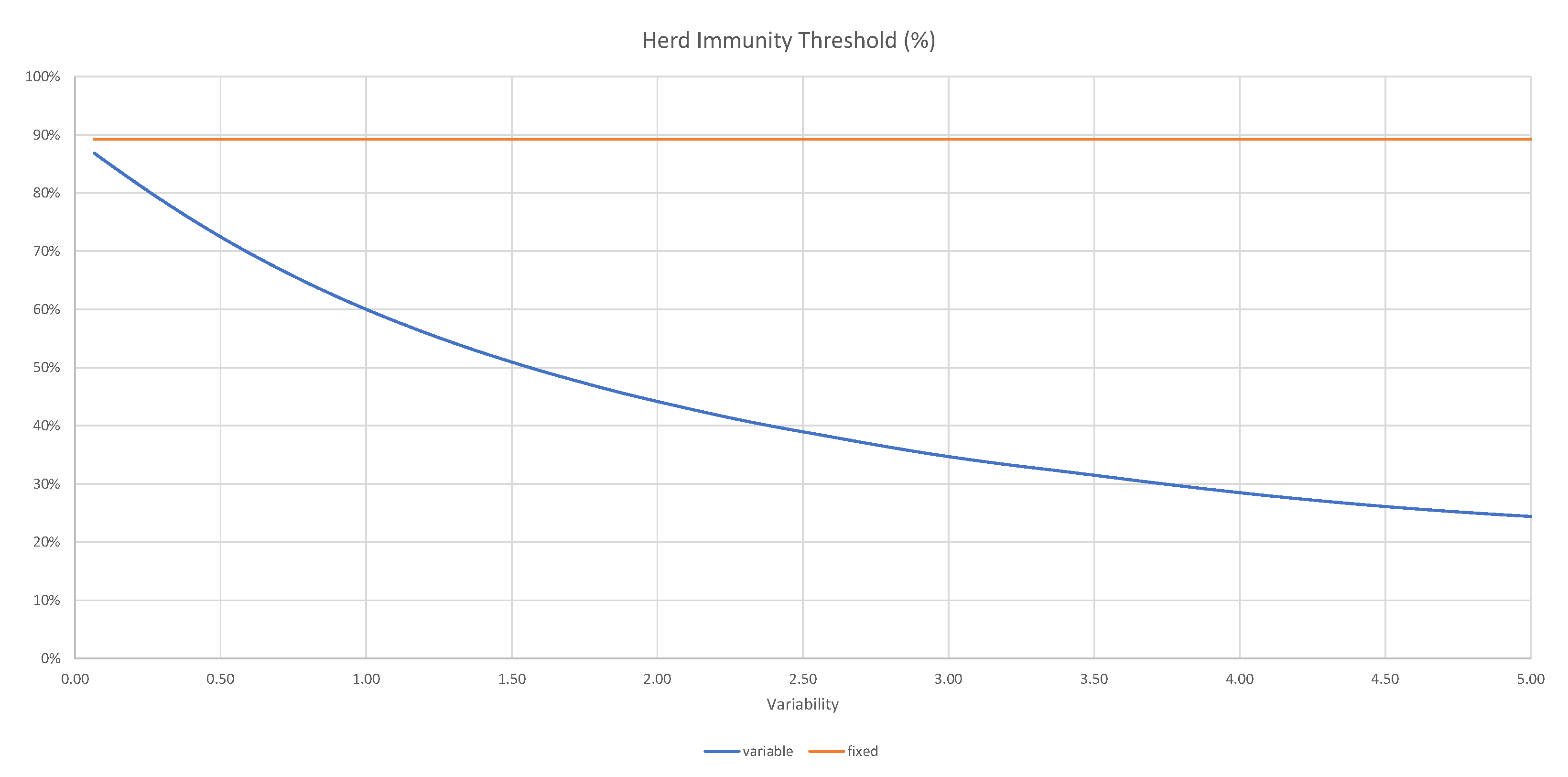
The values of $s\left(\mathfrak{R},\alpha \right)$ as a function of variability ${\alpha }^{-1}$ for a given $\mathfrak{R}$ are shown in Figure 16.

We also show the limiting value $s\left(\mathfrak{R}\right)\equiv s\left(\mathfrak{R},\infty \right)$ corresponding to the deterministic susceptibility. It follows from Equation (40) that $s\left(\mathfrak{R}\right)$ solves the following equation:

$$lns\left(\mathfrak{R}\right)+\mathfrak{R}\left(1-s\left(\mathfrak{R}\right)\right)=0.$$

(42)

Figure 16 clearly shows that the variability plays a very important role in determining the level of herd immunity, which can be achieved with a much lower number of infected.

5.7. Finite ICU Capacity and Its Implications

One of the most fundamental and novel aspects of our model is the fact that it is capable of accounting for the potential supply–demand imbalance of the ICU cases, which can be critical for overall mortality.

In fact, one of the main arguments in favor of the lockdown of several major economies is that such a lockdown prevents the potential collapse of the healthcare system.

We shall show below that, given a relatively modest ICU overcapacity, such a collapse is highly unlikely, even if only a partial lockdown on a high-risk population is implemented instead.

We model the overflow of the ICU utilization by adjusting coefficients $\delta$:

$$\begin{array}{ccc}\hfill {\delta }_k^{\left(H\right)}& =& {\overline{\delta }}_k^{\left(H\right)}\mathcal{H}\left(C-{\sum }_{\overline{k}=1}^K{V}_{\overline{k}}\right),\hfill \\ \hfill {\delta }_k^{\left(D\right)}& =& {\overline{\delta }}_k^{\left(D\right)}+{\overline{\delta }}_k^{\left(H\right)}\left(1-\mathcal{H}\left(C-{\sum }_{\overline{k}=1}^K{V}_{\overline{k}}\right)\right).\hfill \end{array}$$

(43)

where $\mathcal{H}\left(.\right)$ is the Heaviside step function. Thus, when the system operates below its capacity, there is no need to ration medical services.

5.8. Description of the Lockdown

The lockdown effects can be modeled by the reduction in the reproductive number, ${\mathfrak{R}}_{0,k}$. Since in addition to these effects we also want to model seasonality, which is a common feature of many viral infections, we allow for ${\mathfrak{R}}_{0,k}$ to be time dependent. The lockdown starts at time ${\chi }_1$, and ends at time ${\chi }_2$. We assume that the reduction in ${\mathfrak{R}}_{0,k}$ as a result of lockdown is in the order of 30–40%.

To model these effects, the coefficients ${\mathfrak{R}}_k\left(t\right)$ have to be made time dependent:

$${\mathfrak{R}}_k\left(t\right)={\varphi }_k\left(t\right){\chi }_k\left(t\right){\mathfrak{R}}_k^{\left(0\right)},$$

(44)

with

$${\varphi }_k\left(t\right)=\sum _{l=1}^L{\overline{\varphi }}_{k,l}\mathcal{H}\left(\left(t-t_{l-1}\right)\left(t_l-t\right)\right).$$

(45)

Here ${\chi }_k\left(t\right)$ is given by Equation (17), $T_0=0$, $T_1...T_{L-1}$, $T_L=T$, and T is the terminal time for the calculation, e.g., $T=365$ days, and $T_1...T_{L-1}$ are times when lockdowns are either imposed or lifted. When there is only a one-time lockdown, we have $L=3$; $T_1$ is the time when it is imposed, and $T_2$ is the time when it is lifted, $T_3=T$. In general, several consecutive rounds of imposing/lifting lockdowns can be contemplated.

When ${\mathfrak{R}}_k\left(t\right)$ are time dependent, Equations (18) and (20) become

$$\begin{array}{ccc}\hfill {\mathsf{\Theta }}_k& =& {\pi }_k\frac{I_k}{N_k}+\left(1-{\pi }_k\right)\mathsf{\Omega },\hfill \\ \hfill \mathsf{\Omega }& =& \frac{{\sum }_{\overline{k}=1}^K{\mathfrak{R}}_{\overline{k}}\left(t\right){\tilde{I}}_{\overline{k}}}{{\sum }_{\overline{k}=1}^K{\mathfrak{R}}_{\overline{k}}\left(t\right){\tilde{N}}_{\overline{k}}},\hfill \end{array}$$

(46)

$$\begin{array}{ccc}\hfill {\mathsf{\Theta }}_k^{\left(\varpi \right)}& =& {\pi }_k\frac{I_k}{N_k^{1-\varpi }}+\left(1-{\pi }_k\right){\mathsf{\Omega }}^{\left(\varpi \right)},\hfill \\ \hfill {\mathsf{\Omega }}^{\left(\varpi \right)}& =& \frac{{\sum }_{\overline{k}=1}^K{\mathfrak{R}}_{\overline{k}}\left(t\right){\tilde{I}}_{\overline{k}}}{{\left({\sum }_{\overline{k}=1}^K{\mathfrak{R}}_{\overline{k}}\left(t\right){\tilde{N}}_{\overline{k}}\right)}^{1-\varpi }},\hfill \end{array}$$

(47)

respectively.

6. Lives vs. Lives

Typically, even modest proposals to end lockdowns are faced with stiff opposition, arguing that lives are being traded for the sake of the economy. Reality is more subtle. While quarantines, which are imminently reasonable, affect a relatively small fraction of the population at a time by isolating sick members of the public, lockdowns, being a blunt tool affecting the community as a whole, have a profound impact on mortality. In Atlas et al. (2020), the authors argue that unemployment and reduction in health care provision inevitably caused by lockdowns result in excess mortality on their own. To account for the adverse effects of lockdowns, we need to generalize the K-SEIR model by introducing the excess mortality ${\mu }_k$, affecting the population as a whole. The corresponding equations have the form

$$\begin{array}{ccc}\hfill \frac{d{S}_k}{dt}& =& -\frac{{\mathfrak{R}}_k}{{\tau }_I}{\mathsf{\Theta }}_k{S}_k-{\mu }_k\left(t\right)S_k,\hfill \\ \hfill \frac{d{E}_k}{dt}& =& \frac{{\mathfrak{R}}_k}{{\tau }_I}{\mathsf{\Theta }}_k{S}_k+\frac{{\mathfrak{R}}_k}{{\tau }_I}{\mathsf{\Theta }}_k{Q}_k-\frac{1}{{\tau }_E}{E}_k,\hfill \\ \hfill \frac{d{I}_k}{dt}& =& \frac{1}{{\tau }_E}{E}_k-\frac{1}{{\tau }_I}{I}_k,\hfill \\ \hfill \frac{d{H}_k}{dt}& =& \frac{{\beta }_k^{\left(H\right)}}{{\tau }_I}{I}_k-\frac{1}{{\tau }_H}{H}_k,\hfill \\ \hfill \frac{d{V}_k}{dt}& =& \frac{{\gamma }_k^{\left(V\right)}}{{\tau }_H}{H}_k-\frac{1}{{\tau }_V}{V}_k,\hfill \\ \hfill \frac{d{D}_k}{dt}& =& \frac{{\beta }_k^{\left(D\right)}}{{\tau }_I}{I}_k+\frac{{\gamma }_k^{\left(D\right)}}{{\tau }_H}{H}_k+{\mu }_k{Q}_k,\hfill \\ \hfill N_k\left(t\right)& =& N_k\left(0\right)-D_k\left(t\right),\hfill \end{array}$$

(48)

7. Delay Difference Equations

It is clear that the standard differential equations are not good enough to describe the actual epidemiological problem at hand because delays between exposure and infection, etc., play a major role in the progression of the disease. Thus, at the very least, we have to use delay differential equations to describe the problem at hand.

Yet, in order to account for the discrete (and very noisy) nature of the observations we are dealing with, it is best to use delay difference equations, adding stochasticity as needed. To this end, we introduce discretely observed variables $S_{k,n},e_{k,n},$etc. We emphasize an important difference between the continuously monitored variables $S,E,I,...$, and discretely monitored variables $S,e,i,...$. While I (say) represents the total number of infected at time t, $i_n$ represents the number of people newly infected at time t. Loosely speaking,

$$i_n=\frac{I_n}{{\tau }_I}.$$

(49)

With this understanding in mind, we can write the system of delayed differential equations (DDEs) as follows:

$$\begin{array}{ccc}\hfill S_{k,n+1}& =& \left(1-\frac{{\mathfrak{R}}_{{}_k}}{{\tau }_I}{\mathsf{\Theta }}_{k,n}\right)S_{k,n},\hfill \\ \hfill e_{k,n+1}& =& \frac{{\mathfrak{R}}_{{}_k}}{{\tau }_I}{\mathsf{\Theta }}_{k,n}{S}_{k,n},\hfill \\ \hfill i_{k,n+1}& =& e_{k,n+1-{\tau }_E},\hfill \\ \hfill h_{k,n+1}& =& {\beta }_k^{\left(H\right)}{i}_{k,n+1-{\tau }_I},\hfill \\ \hfill d_{k,n+1}& =& {\beta }_k^{\left(D\right)}{i}_{k,n+1-{\tau }_I}+{\gamma }_k^{\left(D\right)}{h}_{k,n+1-{\tau }_H},\hfill \end{array}$$

(50)

where

$$\begin{array}{ccc}\hfill {\mathsf{\Theta }}_{k,n}& =& {\pi }_k\frac{I_{k,n}}{N_{k,n}^{1-\varpi }}+\left(1-{\pi }_k\right)\frac{\left({\mathfrak{R}}_1{\tilde{I}}_{1,n}+{\mathfrak{R}}_2{\tilde{I}}_{2,n}\right)}{{\left({\mathfrak{R}}_1{\tilde{N}}_{1,n}+{\mathfrak{R}}_2{\tilde{N}}_{2,n}\right)}^{1-\varpi }},\hfill \\ \hfill I_{k,n}& =& \sum _{m=n-{\tau }_I}^n{i}_{k,n},{\tilde{I}}_{k,n}=\left(1-{\pi }_k\right)I_{k,n},\hfill \\ \hfill N_{k,n}& =& N_{k,0}-D_{k,n},{\tilde{N}}_{k,n}=\left(1-{\pi }_k\right)N_{k,n}.\hfill \end{array}$$

(51)

It is more appropriate to treat times ${\tau }_{\alpha }$, $\alpha =E,I,H$, as discrete random variables with pdfs $f_{\alpha }\left(.\right)$ and cdfs $F_{\alpha }\left(.\right)$, rather than given constants. The corresponding randomized delayed difference equations (RDDEs) have the form

$$\begin{array}{ccc}\hfill S_{k,n+1}& =& \left(1-\frac{{\mathfrak{R}}_{{}_k}}{{\tau }_I}{\mathsf{\Theta }}_{k,n}\right)S_{k,n},\hfill \\ \hfill e_{k,n+1}& =& \frac{{\mathfrak{R}}_{{}_k}}{{\tau }_I}{\mathsf{\Theta }}_{k,n}{S}_{k,n},\hfill \\ \hfill i_{k,n+1}& =& \sum _{m=0}^{n+1}{e}_{k,n+1-m}{f}_E\left(m\right),\hfill \\ \hfill h_{k,n+1}& =& {\beta }_k^{\left(H\right)}\sum _{m=0}^{n+1}{i}_{k,n+1-m}{f}_E\left(m\right),\hfill \\ \hfill d_{k,n+1}& =& {\beta }_k^{\left(D\right)}\sum _{m=0}^{n+1}{i}_{k,n+1-m}{f}_E\left(m\right)+{\gamma }_k^{\left(D\right)}\sum _{m=0}^{n+1}{h}_{k,n+1-m}{f}_H\left(m\right),\hfill \end{array}$$

(52)

where

$$\begin{array}{ccc}\hfill {\mathsf{\Theta }}_{k,n}& =& {\pi }_k\frac{I_{k,n}}{N_{k,n}^{1-\varpi }}+\left(1-{\pi }_k\right)\frac{\left({\mathfrak{R}}_1{\tilde{I}}_{1,n}+{\mathfrak{R}}_2{\tilde{I}}_{2,n}\right)}{{\left({\mathfrak{R}}_1{\tilde{N}}_{1,n}+{\mathfrak{R}}_2{\tilde{N}}_{2,n}\right)}^{1-\varpi }},\hfill \\ \hfill I_{k,n}& =& \sum _{m=0}^n{i}_{k,m}{F}_I\left(m\right),{\tilde{I}}_{k,n}=\left(1-{\pi }_k\right)I_{k,n},\hfill \\ \hfill N_{k,n}& =& N_{k,0}-D_{k,n},{\tilde{N}}_{k,n}=\left(1-{\pi }_k\right)N_{k,n}.\hfill \end{array}$$

(53)

8. Calibration

8.1. Calibration of the SIR Model

The flow chart describing the progress of the disease is an obvious simplification of the one shown in Figure 5. The corresponding dynamic equations can be written in the form of delay differential–difference equations similar to Equation (3):

$$\begin{array}{ccc}\hfill \frac{ds\left(t\right)}{dt}& =& -\frac{\mathfrak{R}i\left(t\right)s\left(t\right)}{{\tau }_I},\hfill \\ \hfill \frac{di\left(t\right)}{dt}& =& \frac{\left(\mathfrak{R}s\left(t\right)-1\right)i\left(t\right)}{{\tau }_I},\hfill \\ \hfill d\left(t\right)& =& {\beta }^{\left(D\right)}\left(1-s\left(t-{\tau }_D\right)\right),\hfill \end{array}$$

(54)

where $s\left(t\right)$, $i\left(t\right)$, $d\left(t\right)$ are susceptible, infected, and deceased fractions of the initial population at time t, ${\beta }^{\left(D\right)}$ is the probability of dying after becoming exposed to the disease, and ${\tau }_D$ is the time between exposure and death; see, for example, Lourenço et al. (2020). The corresponding initial conditions are

$$s\left(\zeta \right)=1-i_0,i\left(\zeta \right)=i_0,$$

(55)

where $\zeta$ is the start time of the outbreak. These equations assume that there is homogeneous mixing among members of the public. This is clearly a gross simplification, which might be justified in some simple situation, but is hardly applicable in the general case.

The governing Equation (54) is very simple and can be solved analytically. The first two equations yield

$$\frac{di}{ds}=-1+\frac{1}{\mathfrak{R}s},$$

(56)

so that

$$\begin{array}{ccc}\hfill i& =& i_0+\left(1-s\right)+\frac{1}{\mathfrak{R}}ln\left(s\right),\hfill \\ \hfill \frac{dt}{{\tau }_I}& =& -\frac{ds}{\left(\mathfrak{R}\left(i_0+\left(1-s\right)\right)+ln\left(s\right)\right)s}.\hfill \end{array}$$

(57)

Let $\overline{s}=1-s$, and

$$\mathsf{\Phi }\left(\overline{s};i_0,\mathfrak{R}\right)=\underset{0}{\overset{\overline{s}}{\int }}\frac{d\overline{s}}{\left(\mathfrak{R}\left(i_0+\overline{s}\right)+ln\left(1-\overline{s}\right)\right)\left(1-\overline{s}\right)}\approx \frac{ln\left(\frac{\left(\mathfrak{R}{i}_0+\left(\mathfrak{R}-1\right)\overline{s}\right)}{\mathfrak{R}{i}_0\left(1-s\right)}\right)}{\left(\mathfrak{R}{i}_0+\left(\mathfrak{R}-1\right)\right)}.$$

(58)

The limit of integration is $\overline{S}$, which satisfies the following equation

$$\mathfrak{R}\left(i_0+\overline{S}\right)+ln\left(1-\overline{S}\right)=0.$$

(59)

This is the asymptotic level for $t\to \infty$ at which the herd immunity is reached.

Accordingly,

$$\overline{s}\left(t\right)=\mathsf{\Psi }\left(\iota ;i_0,\mathfrak{R}\right)\approx \frac{\mathfrak{R}{i}_0{e}^{\left(\mathfrak{R}{i}_0+\left(\mathfrak{R}-1\right)\right)\iota }}{\mathfrak{R}{i}_0{e}^{\left(\mathfrak{R}{i}_0+\left(\mathfrak{R}-1\right)\right)\iota }+\left(\mathfrak{R}-1\right)}\approx \frac{\mathfrak{R}{i}_0{e}^{\left(\mathfrak{R}-1\right)\iota }}{\left(\mathfrak{R}-1\right)},$$

(60)

where $\iota =\left(t-\zeta \right)/{\tau }_I$, and $\mathsf{\Psi }$ is the inverse of the $\mathsf{\Phi }$ function. Thus, $\overline{s}\left(t\right)$ has a universal shape which depends on the disease-specific parameters $\mathfrak{R},{\tau }_I$ and the initial fraction of the infected population. Finally,

$$D\left(t\right)={\beta }^{\left(D\right)}\mathsf{\Psi }\left(\iota ;i_0,\mathfrak{R}\right)N_0\approx {\beta }^{\left(D\right)}\frac{\mathfrak{R}{e}^{\left(\mathfrak{R}-1\right)\iota }}{\left(\mathfrak{R}-1\right)}{I}_0,$$

(61)

where $I_0=i_0{N}_0$ is the initial number of infected individuals. We emphasize that in the beginning, the death toll $D\left(t\right)$ is independent of the size of the overall population such that the conclusions drawn in Lourenço et al. (2020) are unverifiable at best.

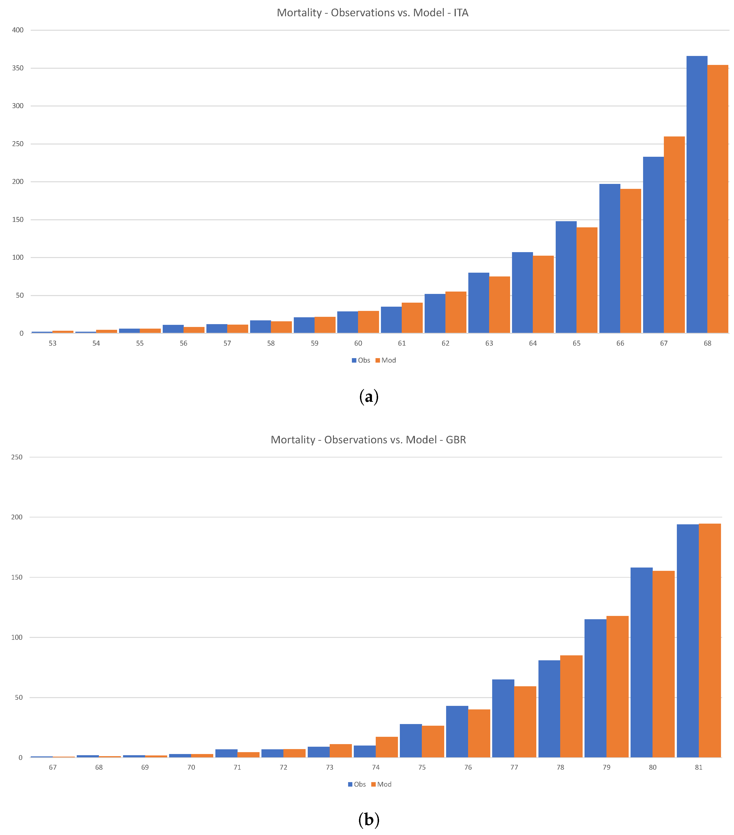
Figure 17 shows how Equation (54) can be calibrated to the initial phase of the disease in Italy and the U.K.

Loureco et al. drew a rather dramatic conclusion from similar calculations; see Lourenço et al. (2020). However, we feel that there is little actual substance in their claims. First, the number of infected individuals in the early stages of the disease is growing both organically and is imported from abroad. Even more importantly, there is absolutely no reason to assume that the overall size of a given country determines the size of the infected population. As we have shown above, the variability of the reproductive number has a profound effect on the ultimate size of the infected population.

8.2. Calibration of the 1-SEIR Model

The reproductive number $\mathfrak{R}\left(t\right)$ is an implied quantity. To start with, let us consider the reduced one-group case. We have

$$\begin{array}{ccc}\hfill \frac{dS\left(t\right)}{dt}& =& -\frac{\mathfrak{R}\left(t\right)}{{\tau }_I}\frac{S\left(t\right)I\left(t\right)}{\left(N_0-D\left(t\right)\right)},\hfill \\ \hfill \frac{dE\left(t\right)}{dt}& =& \frac{\mathfrak{R}\left(t\right)}{{\tau }_I}\frac{S\left(t\right)I\left(t\right)}{\left(N_0-D\left(t\right)\right)}-\frac{1}{{\tau }_E}E\left(t\right),\hfill \\ \hfill \frac{dI\left(t\right)}{dt}& =& \frac{1}{{\tau }_E}E\left(t\right)-\frac{1}{{\tau }_I}I\left(t\right),\hfill \\ \hfill \frac{dD\left(t\right)}{dt}& =& \frac{{\beta }^{\left(D\right)}}{{\tau }_I}I\left(t\right),\hfill \end{array}$$

(62)

Since we are interested in matching the hospital admissions and the deaths, the equation for $R\left(t\right)$ is redundant. We also emphasize that the number of cases is not worth calibrating to because it is extremely unreliable.

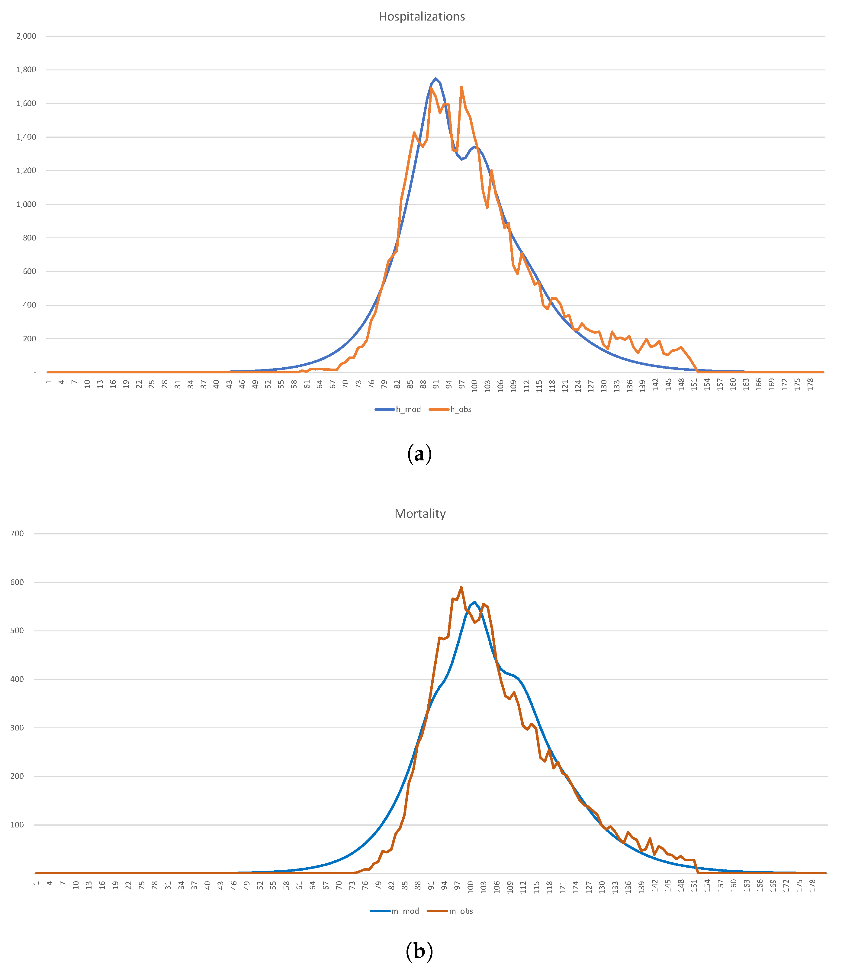
In Figure 18, we show the calibration of the 1-SEIR model to the hospitalization and death statistics in New York City.

The corresponding parameters, which are in broad agreement with Table 2 and Table 3, have the form

$$\begin{array}{ccc}\hfill {\tau }_E& =& 6d,{\tau }_I=7d,{\tau }_H=10d,\hfill \\ \hfill {\beta }^{\left(H\right)}& =& 2.45\%,{\beta }^{\left(R\right)}=97.31\%,{\beta }^{\left(D\right)}=0.24\%,\hfill \\ \hfill {\gamma }^{\left(R\right)}& =& 74.73\%,{\gamma }^{\left(D\right)}=25.27\%,\hfill \\ \hfill R_0^{<}& =& 2.35,R_0^{>}=0.97,\varpi =0.0420.\hfill \end{array}$$

(63)

Because of the effects of variability, which we discussed earlier, it is unreasonable to assume that $N\left(0\right)=$ 8,200,000, i.e., the entire population of the city. Instead, we view it as a variable quantity, which is chosen in such a way that in the long-run proportion of the population, infected with the virus at some point in time, equals $25\%$ of $N\left(0\right)$, or 2,050,000, say. As a result, the “effective” $\overline{N}\left(0\right)=$ 2,450,000. If so desired, one can run the calibration with the actual $N\left(0\right)$. Results change in the obvious fashion—the burden of the disease becomes much less, but the number of affected individuals is much larger. The number of infected individuals on 1 January 2020 is 14. The case mortality rate is $0.86\%$.

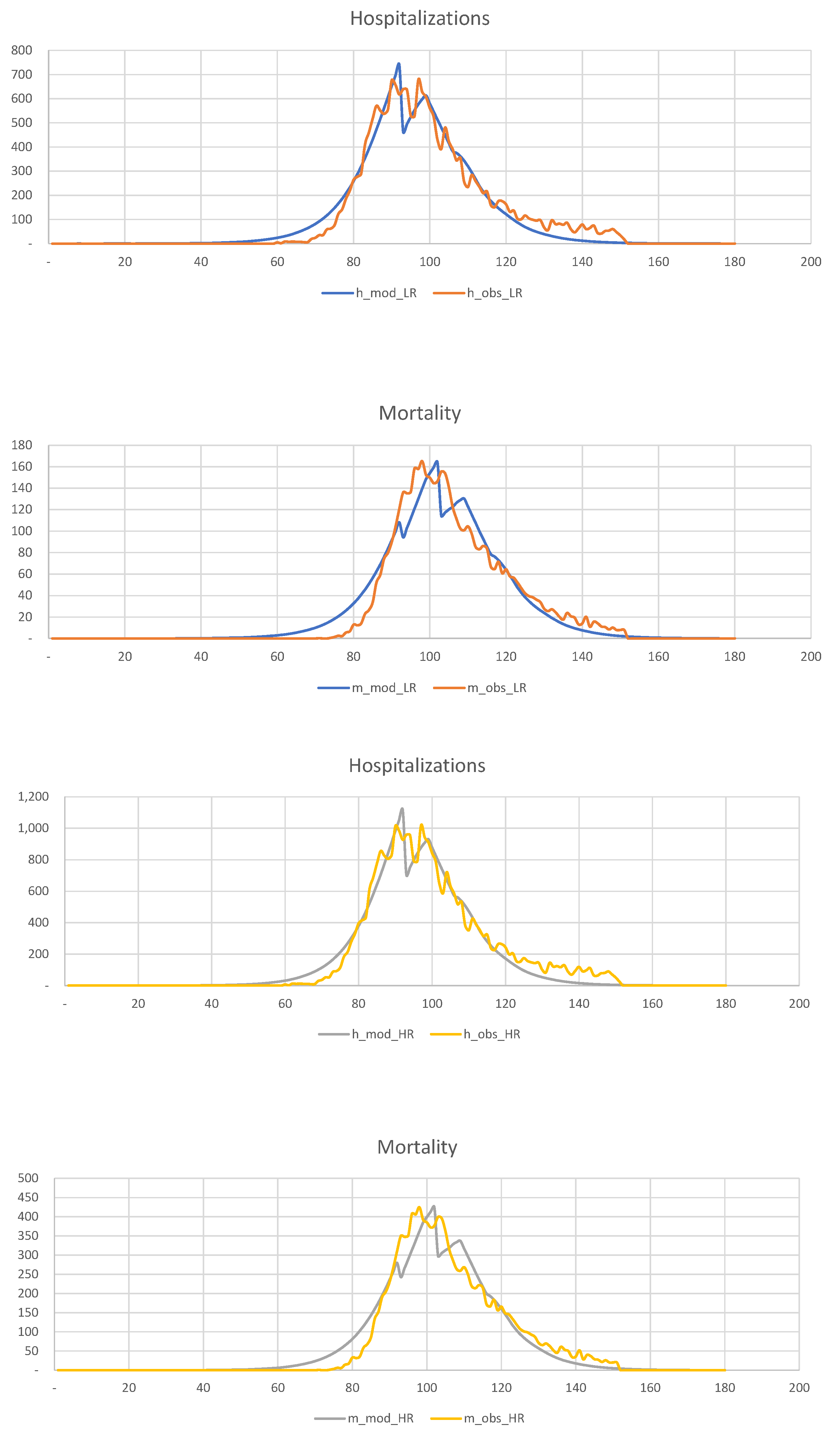
8.3. Calibration of the 2-SEIR Model

Consider now the case $K=2$, so that there are only two groups: (a) the low-risk class (LR, or group 1); (b) the high-risk class (HR, or group 2). Since age is the most, albeit not the only, important determinant, we can assume that relative sizes of the groups are 9:1.

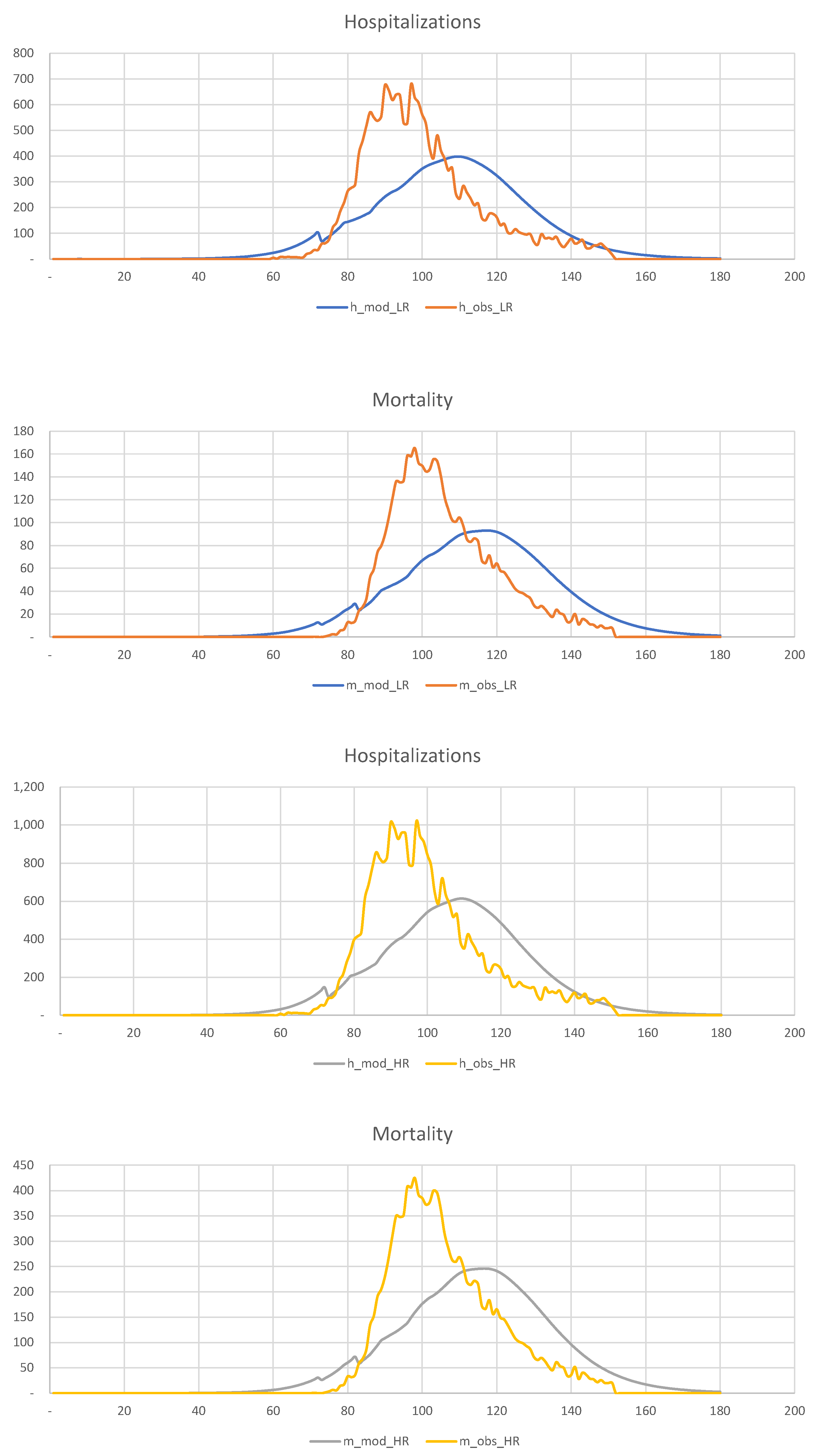
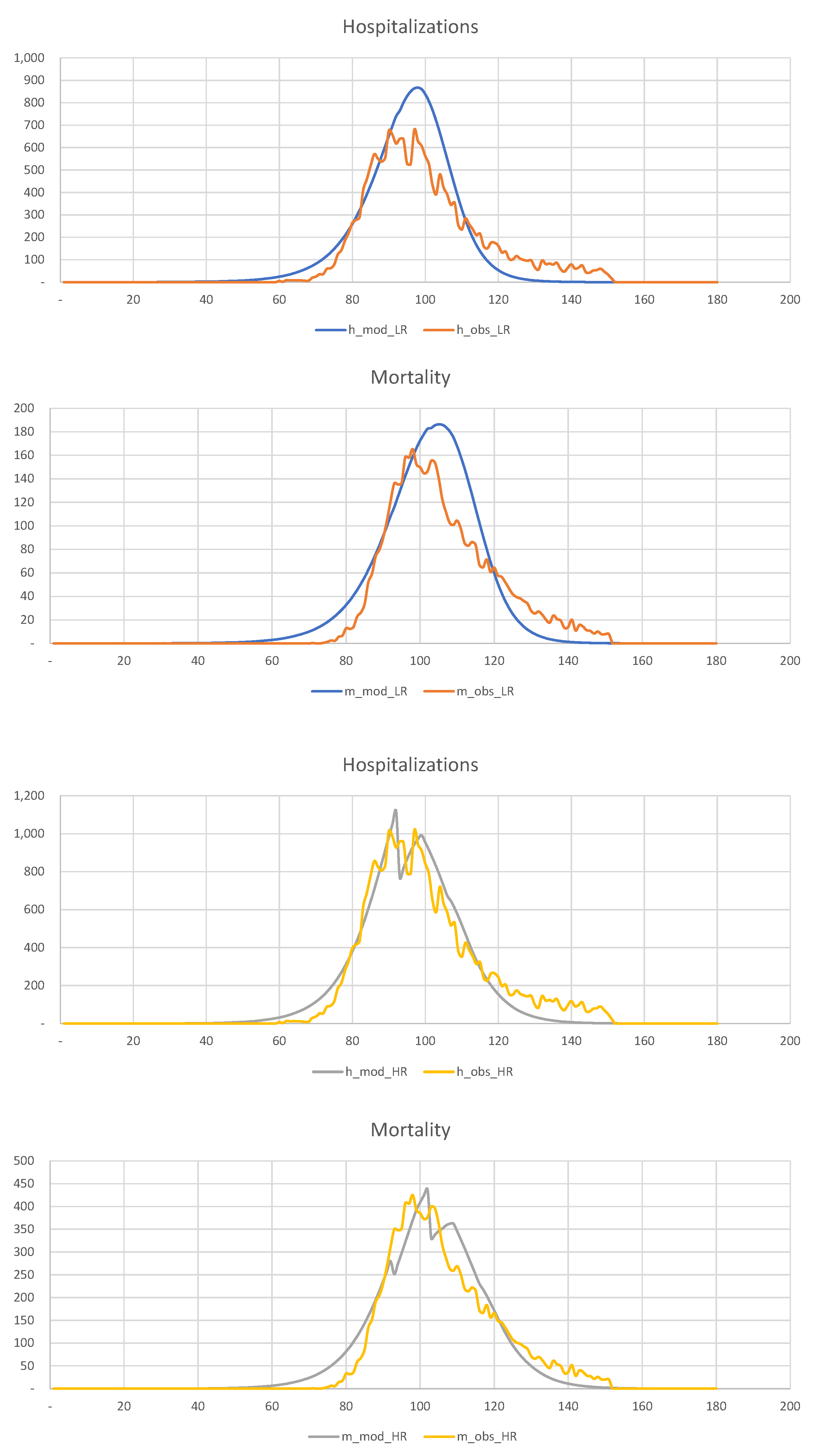
The corresponding equations have the form Equation (14) with $K=2$. In Figure 19, we show the results of the calibration of the 2-SEIR model to the hospitalization and death statistics in New York City.

We divide the entire population into two groups, $N_{LR}\left(0\right)=$ 6,970,000, $N_{HR}\left(0\right)=$ 1,230,000, and calculate the corresponding “effective” sizes, ${\overline{N}}_{LR}\left(0\right)=$ 1,952,000, ${\overline{N}}_{HR}\left(0\right)=$ 428,000, in such a way that the total number of infected individuals is 2,050,000. The relevant parameters are shown below

$$\begin{array}{ccc}\hfill {\tau }_E& =& 6d,{\tau }_I=7d,{\tau }_H=10d,\hfill \\ \hfill {\beta }_{LR}^{\left(H\right)}& =& 1.19\%,{\beta }_{LR}^{\left(R\right)}=98.72\%,{\beta }_{LR}^{\left(D\right)}=0.09\%,\hfill \\ \hfill {\gamma }_{LR}^{\left(R\right)}& =& 82.77\%,{\gamma }_{LR}^{\left(D\right)}=17.23\%,\hfill \\ \hfill R_{0,LR}^{<}& =& 1.73,R_{0,LR}^{>}=1.14,{\varpi }_{LR}=0.0379,{\pi }_{LR}=80.00\%,\hfill \\ \hfill {\beta }_{HR}^{\left(H\right)}& =& 7.93\%,{\beta }_{HR}^{\left(R\right)}=91.07\%,{\beta }_{HR}^{\left(D\right)}=1.00\%,\hfill \\ \hfill {\gamma }_{HR}^{\left(R\right)}& =& 70.71\%,{\gamma }_{HR}^{\left(D\right)}=29.29\%,\hfill \\ \hfill R_{0,HR}^{<}& =& 1.85,R_{0,HR}^{>}=1.23,{\varpi }_{HR}=0.0379,{\pi }_{HR}=80.00\%.\hfill \end{array}$$

(64)

It is clear that the LR and HR groups’ mortality rates are very different, 0.29% for the LR group, and 3.33% for the HR group. Overall, COVID-19 mortality is of order 0.84%, as we saw before.

9. Lockdown Strategies—Pros and Cons

Once we manage to calibrate the 2-SEIR model to the New York City data, we can use the corresponding parameters to investigate the following essential questions:

• Can early quarantine save lives?
• Did the actual quarantine save lives?
• Is there any benefit in imposing a quarantine on the low-risk population?

We present the answer to the above questions graphically in Figure 20, Figure 21 and Figure 22.

In Figure 20, we show the hospitalization and mortality statistics for the low-risk and high-risk populations, assuming that quarantine is imposed three weeks earlier than in reality, i.e., on the 60th day of the year, rather than the 80th.

This figure shows that early detection of disease and intervention is the most efficient way of dealing with the pandemic in such densely populated areas as New York. The experience with Los Angeles is another excellent example. However, because of the difficulties with data collection and other considerations, this is often impossible. Our observations are in agreement with Pei et al. (2020).

In Figure 21, we show the hospitalization and mortality statistics for the low-risk and high-risk populations assuming that no quarantine is imposed.

This figure shows that late quarantine is not an efficient way of dealing with the pandemic in such densely populated areas as New York.

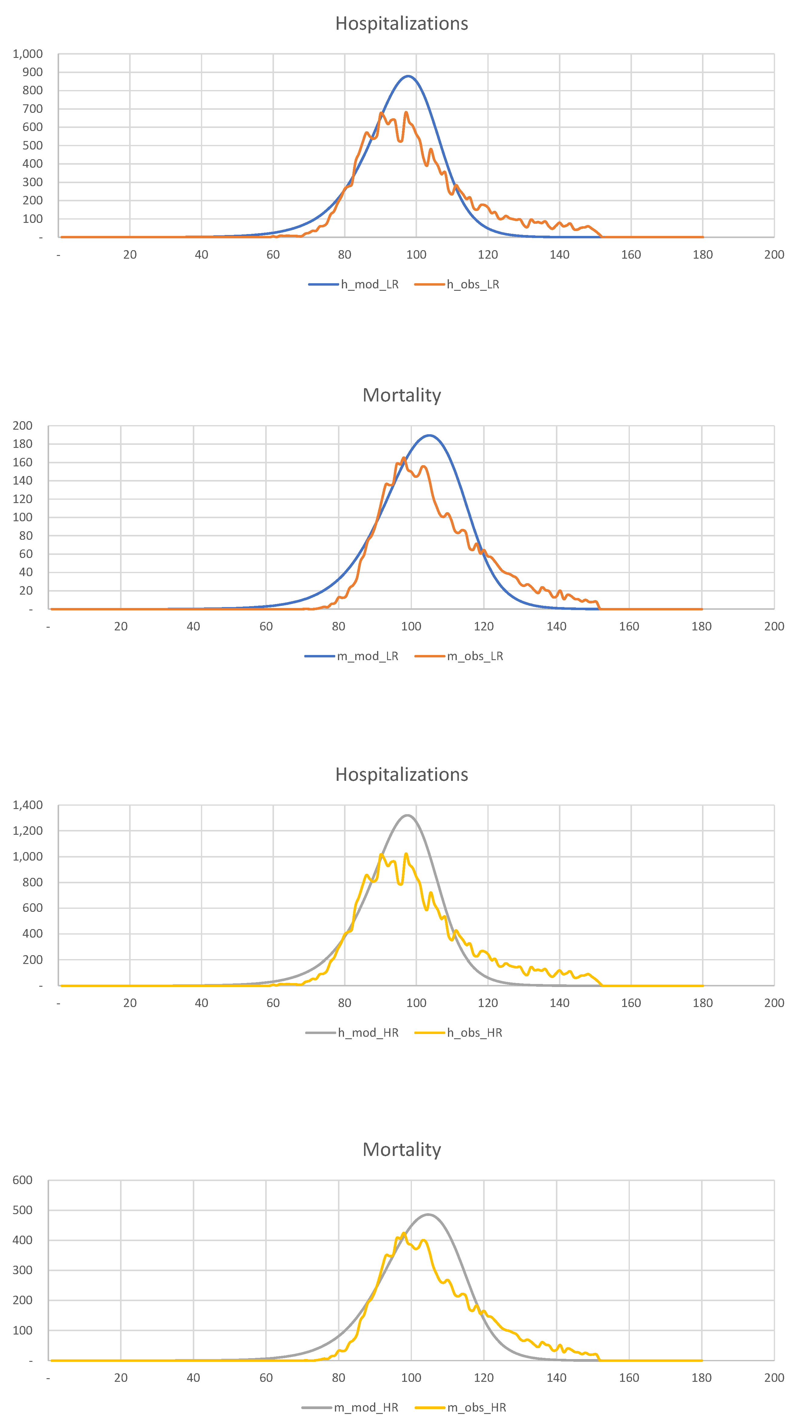
Finally, in Figure 22, we show hospitalization and mortality statistics for the low-risk and high-risk populations, assuming that no quarantine is imposed on the low-risk population. This figure shows that late quarantine is not an efficient way of dealing with the pandemic in such densely populated areas as New York. Thus, there is no discernible difference between quarantining and not quarantining the low-risk population.

In summary, a late quarantine is not an efficient tool for mitigating the consequences of the COVID-19 pandemic in a densely populated urban area.

10. Learning from the Swedish Experience

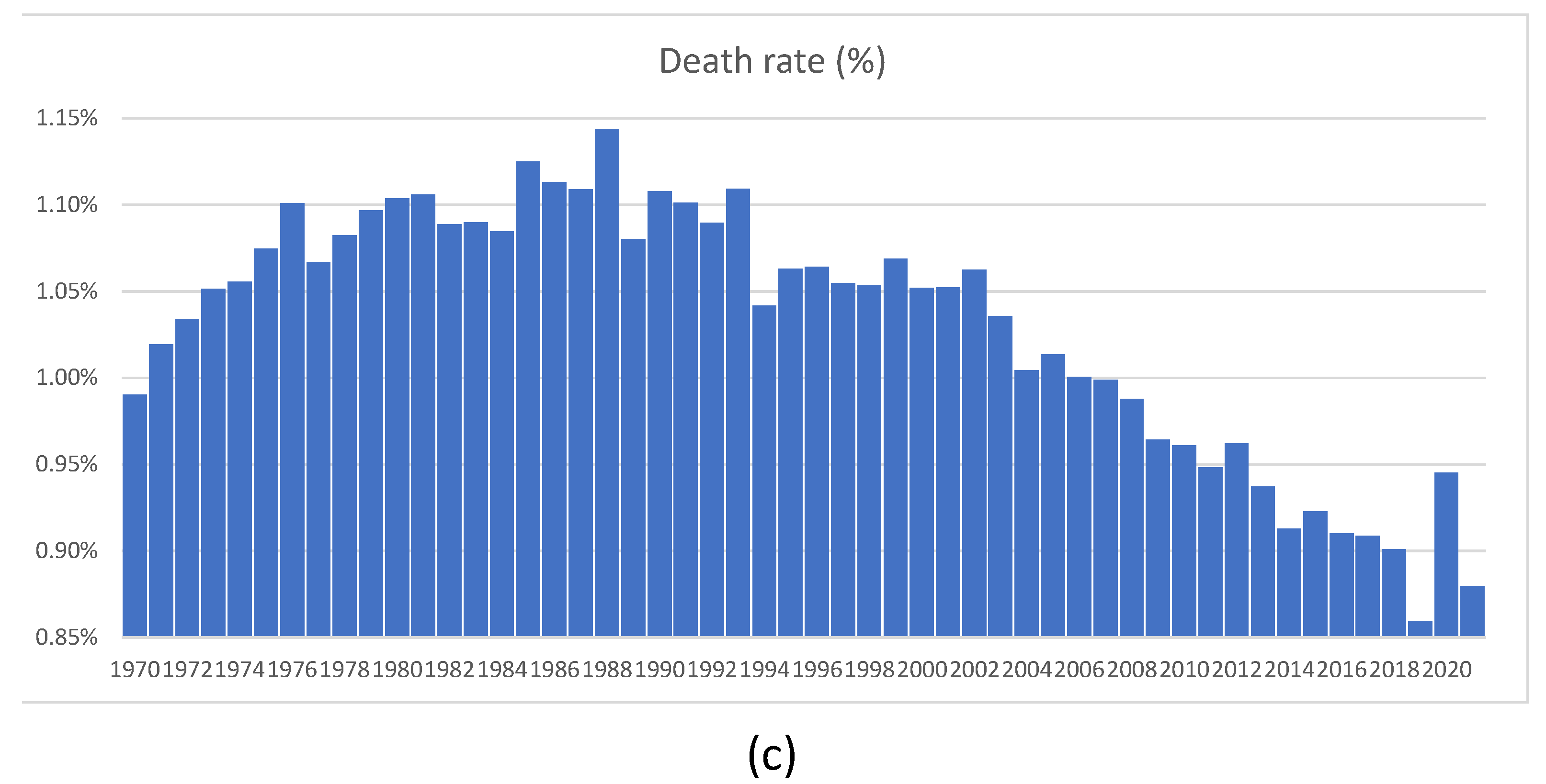
In this section, we briefly discuss the so-called “Swedish experience”. Recall that at the beginning of the pandemic, the Swedish authorities refused to follow the rest of the world, including their Scandinavian neighbors, and did not introduce lockdowns. Instead, they introduced a series of largely voluntary measures to reduce the transmission of the virus. Ever since they chose this “non-standard” (but imminently reasonable) course of action, many newspaper articles and talk shows were dedicated to elucidating what was wrong with the Swedish approach. Finally, after two years, we can see the consequences of not introducing lockdowns in Sweden. Thanks to the exceptionally comprehensive mortality statistics accumulated by Statistics Sweden, founded in 1858, we can look at the number of deaths in 2020 and 2021 in the proper historical context.

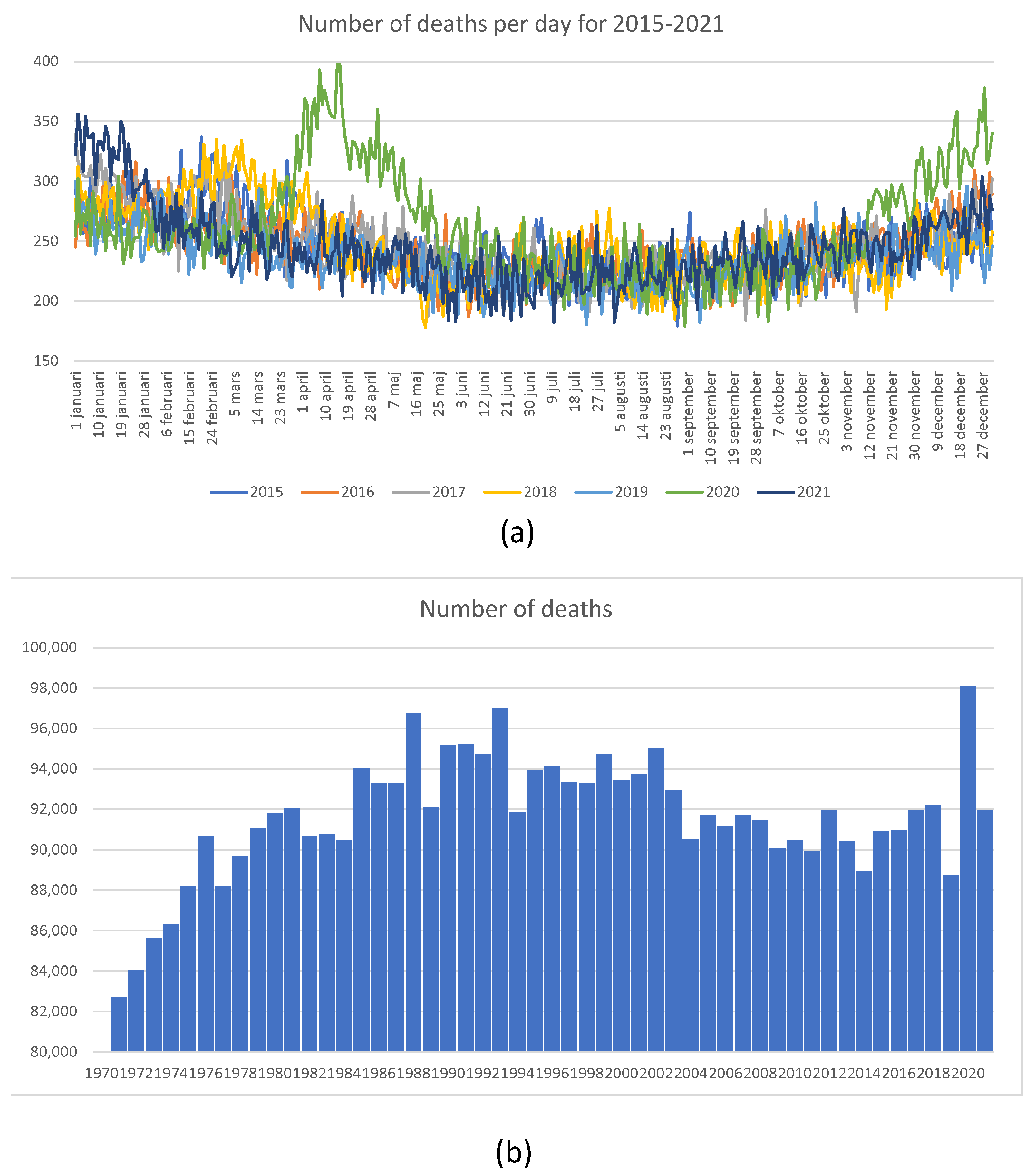
In Figure 23, we show mortality statistics for Sweden in retrospective.

Figure 23a shows the total number of deaths per day for 2015–2022. It is clear that in 2020, the number of deaths was elevated in April, May, and June. However, the overall number of deaths shown in Figure 23b looks large when compared with deaths experienced in 2019, when it was quite low. The number of deaths as a proportion of the total population, shown in Figure 23c, was much higher between 1970 and 2012, without generating any publicity or public health measures at all. We feel that the Swedish experience shows that sensible measures are as effective as lockdowns. One error of the Swedish authorities was their delay in isolating nursing homes. The authors of Juul et al. (2021), who compared the Swedish and Norwegian experiences, arrived at similar conclusions.

11. Discussion

This article develops a detailed and rich epidemiological multi-factor model and several simpler models, which we use as its building blocks. The ultimate model is complex enough to account for all the relevant disease propagation features, its disparate impact on different groups in the population, and interactions within and between various groups. In addition, our model accounts for such aspects of a given medical system as the availability (or lack thereof) of spare hospital beds and intensive care units (ICU) to accommodate the pent-up demand due to the pandemic.

In sharp contrast to many previous pandemics, the COVID-19 pandemic has resulted in many asymptomatic cases. As a result, standard epidemiological models have to guess the number of infected patients, which is very hard to do. In contrast, we use the most recent hospitalization and mortality data to calibrate the model.5

In the epidemiological context, calibration R0 to the observable data seems new. It allows one to perform “nowcasting” the mortality and transmissibility of the pandemic. We borrowed this approach from quantitative finance, where implied volatilities and similar quantities are widely popular; see, for example, Lipton (2001).

Our model can achieve meaningful results; however, it is not without limitations. For instance, we completely neglected the geographical aspects of the COVID-19 propagation. In the future, we plan to study an extension of our K-SEIR model, which we call the KL-SEIR model. The latter accounts not just for the stratification across different age groups, etc., but also across different cities and countries.

12. Conclusions

Governments need protocols for “nowcasting” the mortality and transmissibility of the pandemic. For example, a random sample of 1000 individuals would have quickly dispelled the WHO’s assertion that COVID-19 had a fatality rate of 3.4%. In addition, government statistics show that lockdowns have successfully slowed down the spread of COVID-19, reducing the number of deaths directly caused by this disease. However, government statistics do not account for the loss of lives and livelihoods derived from universal lockdowns.

Lockdowns should aim to minimize the total loss of life, and not only deaths directly caused by the pandemic. In particular, large-scale unemployment is a leading cause of drug abuse. Over the following months and years, we will likely observe a spike in drug-abuse-related deaths, crime, and mental health issues.

The K-SEIR model shows that targeted lockdowns (on high-risk populations) are more likely to achieve the triple goal of minimizing loss of life and loss of livelihood, and avoiding the depletion of medical resources. On the other hand, in countries with a well-developed healthcare system and a population willingly abiding by sensible rules and regulations, the sheltering in place of the entire community is excessive and harmful when considered holistically.

A brief universal lockdown is warranted while we collect data regarding mortality and transmissibility, followed by targeted lockdowns of the high-risk population. The low-risk population should continue to practice sensible personal protection measures.

Given the actual nature of the disease we are battling—COVID-19—it is very likely that the schools’ opening does not increase the risk of overcapacity of the health system or the chance for a second wave. At the same time, it is imperative to seal nursing homes as best as possible to avoid a high infection and mortality rate among their clients. It is also essential to implement sensible pandemic response measures, such as wearing face masks, following strict hygiene routines, practicing social distancing, paid-for self-quarantine, testing, and tracking. Frequent testing of essential workers has to be a priority. It is also helpful to issue a clean bill of health to the individuals who have recovered from the virus and developed antibodies, provided that the virus immunity is real.

Governments must learn from the mistakes of COVID-19 management and design targeted lockdowns in anticipation of COVID-20.

We feel that extending our approach and making it more versatile and granular will help fight future pandemics and allow government and medical bodies to make more meaningful and less disruptive decisions. In particular, one cannot overestimate the role of nowcasting in making decisions under uncertainty.

The Matlab code used to perform the calculations is available from the authors upon request.

References

- Acemoglu, Daron, Victor Chernozhukov, Iván Werning, and Michael D. Whinston. 2020. A Multi-Risk Sir Model with Optimally Targeted Lockdown (No. w27102). National Bureau of Economic Research. Available online: https://www.nber.org/papers/w27102 (accessed on 1 June 2020).
- Adams-Prassl, Abi, Teodora Boneva, Marta Golin, and Christopher Rauh. 2020. Inequality in the impact of the coronavirus shock: Evidence from real time surveys. Journal of Public Economics 189: 104245. [Google Scholar] [CrossRef]
- Atlas, Scott W., John R. Birge, Ralph L. Keeney, and Alexander Lipton. 2020. The COVID-19 shutdown will cost Americans millions of years of life. The Hill. May 25. Available online: https://thehill.com/opinion/healthcare/499394-the-covid-19-shutdown-will-cost-americans-millions-of-years-of-life (accessed on 25 May 2020).
- Anderson, Roy M., and Robert M. May. 1992. Infectious Diseases of Humans: Dynamics and Control. Oxford: Oxford University Press. [Google Scholar]
- Birge, John R., Ozan Candogan, and Yi Ding Feng. 2020. Controlling Epidemic Spread: Reducing Economic Losses with Targeted Closures. Becker Friedman Institute for Economics Working Paper, (2020-57). Chicago: University of Chicago, Available online: https://papers.ssrn.com/sol3/papers.cfm?abstract_id=3590621 (accessed on 15 May 2020).
- Brauer, Fred, P. Van Den Driessche, and Jianhong Wu. 2008. Lecture Notes in Mathematical Epidemiology. Berlin: Springer. [Google Scholar]
- Centres for Disease Control and Prevention. 2020. Past Pandemics. Available online: https://www.cdc.gov/flu/pandemic-resources/basics/past-pandemics.html (accessed on 1 April 2020).
- Choe, Seoyun, and Sunmi Lee. 2015. Modeling optimal treatment strategies in a heterogeneous mixing model. Theoretical Biology and Medical Modelling 12: 28. [Google Scholar] [CrossRef] [PubMed]
- Chowell, Gerardo, and James M. Hyman, eds. 2016. Mathematical and Statistical Modeling for Emerging and Re-Emerging Infectious Diseases. Berlin: Springer. [Google Scholar]
- Condon, Bradly John, and Tapen Sinha. 2010. Who is that masked person: The use of face masks on Mexico City public transportation during the Influenza A (H1N1) outbreak. Health Policy 95: 50–56. [Google Scholar] [CrossRef] [PubMed]
- Cowling, B. J., Y. Zhou, D. K. M. Ip, G. M. Leung, and A. E. Aiello. 2010. Face masks to prevent transmission of influenza virus: A systematic review. Epidemiology & Infection 138: 449–56. [Google Scholar]
- Del Valle, Sara Y., Raymond Tellier, Gary S. Settles, and Julian W. Tang. 2010. Can we reduce the spread of influenza in schools with face masks? American Journal of Infection Control 38: 676–77. [Google Scholar] [CrossRef] [PubMed]
- Ferguson, Neil M., Daniel Laydon, Gemma Nedjati-Gilani, Natsuko Imai, and Kylie Ainslie. 2020. Report 9: Impact of Non-Pharmaceutical Interventions (NPIs) to Reduce COVID19 Mortality and Healthcare Demand. Available online: https://www.imperial.ac.uk/media/imperial-college/medicine/sph/ide/gida-fellowships/Imperial-College-COVID19-NPI-modelling-16-03-2020.pdf (accessed on 1 April 2020).
- Gershon, David, Alexander Lipton, and Hagai Levine. 2020. Managing COVID-19 Pandemic without Destroying the Economy. Working Paper. Available online: https://arxiv.org/abs/2004.10324 (accessed on 9 May 2020).
- Gomes, Ricardo Aguas, Rodrigo M. Corder, Jessica G. King, Kate E. Langwig, and Caetano Souto-Maior. 2020. Individual Variation in Susceptibility or Exposure to SARS-CoV-2 Lowers the Herd Immunity Threshold. medRxiv. Available online: https://www.medrxiv.org/content/medrxiv/early/2020/05/21/2020.04.27.20081893.full.pdf (accessed on 1 June 2020).
- Juul, Frederik E., Henriette C. Jodal, Ishita Barua, Erle Refsum, Ørjan Olsvik, Lise M. Helsingen, Magnus Løberg, Michael Bretthauer, Mette Kalager, and Louise Emilsson. 2021. Mortality in Norway and Sweden during the COVID-19 pandemic. Scandinavian Journal of Public Health, 14034948211047137. [Google Scholar] [CrossRef] [PubMed]
- Khalili, Malahat, Mohammad Karamouzian, Naser Nasiri, Sara Javadi, Ali Mirzazadeh, and Hamid Sharifi. 2020. Epidemiological Characteristics of COVID-19: A Systemic Review and Meta-Analysis. medRxiv. Available online: https://www.medrxiv.org/content/10.1101/2020.04.01.20050138v1 (accessed on 15 April 2020).
- Kermack, William Ogilvy, and A. G. McKendrick. 1927. A contribution to the mathematical theory of epidemics. Proceedings of the Royal Society of London. Series A, Containing Papers of a Mathematical and Physical Character 115: 700–21. [Google Scholar]
- Kilbourne, Edwin D. 2006. Influenza pandemics of the 20th century. Emerging Infectious Diseases 12: 9. [Google Scholar] [CrossRef] [PubMed]
- Kissler, Stephen, Christine Tedijanto, Marc Lipsitch, and Yonatan H. Grad. 2020. Social Distancing Strategies for Curbing the COVID-19 Epidemic. medRxiv. Available online: https://www.medrxiv.org/content/10.1101/2020.03.22.20041079v1 (accessed on 30 March 2020).
- Kucharski, Adam J., Timothy W. Russell, and Charlie Diamond. 2020. Early dynamics of transmission and control of COVID-19: A mathematical modelling study. Lancet Infect Disease 20: 553–558. [Google Scholar] [CrossRef] [Green Version]
- Li, Qun, M. Med, Xuhua Guan, Peng Wu, Xiaoye Wang, Lei Zhou, and Yeqing Tong. 2020. Early transmission dynamics in Wuhan, China, of novel coronavirus—Infected pneumonia. New England Journal of Medicin. [Google Scholar] [CrossRef]
- Liu, Xinzhi, and Peter Stechlinski. 2017. Infectious Disease Modeling. Berlin: Springer. [Google Scholar]
- Linton, Natalie M., Tetsuro Kobayashi, Yichi Yang, Katsuma Hayashi, Andrei R. Akhmetzhanov, and Sung-mok Jung. 2020. Incubation period and other epidemiological characteristics of 2019 novel coronavirus infections with right truncation: A statistical analysis of publicly available case data. Journal of Clinical Medicine 9: 538. [Google Scholar] [CrossRef] [PubMed] [Green Version]
- Lipton, Alexander. 2001. Mathematical Methods for Foreign Exchange. Singapore: World Scientific. [Google Scholar]
- Lipton, Alexander, and Marcos Lopez de Prado. 2020a. Three Quant Lessons from COVID-19. Risk Magazine. Available online: https://papers.ssrn.com/sol3/papers.cfm?abstract_id=3580185 (accessed on 21 April 2020).
- Lipton, Alexander, and Marcos Lopez de Prado. 2020b. Exit Strategies for COVID-19: An Application of the K-SEIR Model (Presentation Slides). Working Paper. Available online: https://papers.ssrn.com/sol3/papers.cfm?abstract_id=3579712 (accessed on 22 April 2020).
- Lipton, Alexander, and Marcos Lopez de Prado. 2020c. Mitigation Strategies for COVID-19: Lessons from the K-SEIR Model. Working Paper. Available online: https://papers.ssrn.com/sol3/papers.cfm?abstract_id=3623544 (accessed on 16 June 2020).
- Lourenço, José, Robert Paton, Mahan Ghafar, Moritz Kraemer, Craig Thompson, and Peter Simmonds. 2020. Fundamental Principles of Epidemic Spread Highlight the Immediate Need for Large-Scale Serological Surveys to Assess the Stage of the SARS-CoV-2 Epidemic. medRxiv. Available online: https://www.medrxiv.org/content/medrxiv/early/2020/03/26/2020.03.24.20042291.full.pdf (accessed on 1 April 2020).
- Manfredi, Piero, and Alberto D’Onofrio, eds. 2013. Modeling the Interplay between Human Behavior and the Spread of Infectious Diseases. Berlin: Springer Science & Business Media. [Google Scholar]
- Martcheva, Maia. 2015. An Introduction to Mathematical Epidemiology. New York: Springer, vol. 61. [Google Scholar]
- Pei, Sen, Sasikiran Kandula, and Jeffrey Shaman. 2020. Differential Effects of Intervention Timing on COVID-19 Spread in the United States. medRxiv. Available online: https://www.medrxiv.org/content/10.1101/2020.05.15.20103655v2 (accessed on 1 June 2020).
- Russell, Timothy W., Joel Hellewell, Christopher I. Jarvis, Kevin van Zandvoort, Sam Abbott, and Ruwan Ratnayake. 2020. Estimating the infection and case fatality ratio for coronavirus disease (COVID-19) using age-adjusted data from the outbreak on the Diamond Princess cruise ship, February 2020. Eurosurveillance 25: 2000256. Available online: https://pubmed.ncbi.nlm.nih.gov/32234121/ (accessed on 1 April 2020).
- Shalev-Shwartz, Shai, and Amnon Shashua. 2020. An Exit Strategy from the Covid-19 Lockdown Based on Risk-Sensitive Resource Allocation. Center for Brains, Minds and Machines (CBMM). Available online: https://dspace.mit.edu/bitstream/handle/1721.1/124669/CBMM-Memo-106.pdf?sequence=1&isAllowed=y (accessed on 1 May 2020).
- Salje, Henrik, Cécile Tran Kiem, Noémie Lefrancq, noémie Courtejoie, Paolo Bosetti, and Juliette Paireau. 2020. Estimating the Burden of SARS-CoV-2 in France. Science 369: 208–11. Available online: https://science.sciencemag.org/content/early/2020/05/12/science.abc3517 (accessed on 15 May 2020).
- Thomas-Rüddel, D., J. Winning, P. Dickmann, D. Ouart, A. Kortgen, U. Janssens, and M. Bauer. 2021. Coronavirus disease 2019 (COVID-19): Update for anesthesiologists and intensivists March 2020. Der Anaesthesist 70: 1–10. [Google Scholar]
- Verity, Robert, Lucy C. Okelll, Ilaria Dorigatti, Peter Winskill, Charles Whittaker, and Natsuko Imai. 2020. Estimates of the severity of coronavirus disease 2019: A model-based analysis. The Lancet Infectious Diseases 20: 669–77. Available online: https://www.thelancet.com/journals/laninf/article/PIIS1473-3099(20)30243-7/fulltext (accessed on 5 April 2020).
- Wölfel, Roman, Victor M. Corman, Wolfgang Guggemos, Michael Seilmaier, Sabine Zange, Marcel A. Müller, Daniela Niemeyer, Patrick Vollmar, Camilla Rothe, Michael Hoelscher, and et al. 2020. Clinical Presentation and Virological Assessment of Hospitalized Cases of Coronavirus Disease 2019 in a Travel-Associated Transmission Cluster. MedRxiv. Available online: https://www.medrxiv.org/content/10.1101/2020.03.05.20030502v1 (accessed on 30 March 2020).
- Worldometers. 2020. Available online: https://www.worldometers.info/coronavirus/ (accessed on 1 April 2020).
Figure 1.
Transmissibility vs. fatality rates of various diseases. At this point, these variables are still uncertain for COVID-19. Source:
Thomas-Rüddel et al. (
2021).