The Effect of Index Option Trading on Stock Market Volatility in China: An Empirical Investigation

Abstract

In this study, we examine the effect of introducing SSE 50ETF index options trading on stock market volatility using a panel data evaluation approach. Based on the cross-sectional dependence among international stock indices and macroeconomic indicators, we estimate the counterfactual volatility of the SSE 50 index and find that the introduction of index options reduces stock market volatility significantly in the long term. The primary findings are robust to alternative econometric models, including principal component analysis, GARCH-family model, and LASSO regression. The results of this paper suggest that the introduction of SSE index options provides investors with risk management tools and improves price discovery in the stock market.

1. Introduction

The economic effect of index or options trading on spot market volatility has received long-lasting academic attention over the past decades. Studies show that futures trading provides additional information to the price formation in the equity market with increased price discovery efficiency, thereby reducing spot market volatility. Such an effect is concentrated in periods of intense market volatility, such as the 1987 U.S. stock market crash and the 2007–2009 global financial crisis. However, if investors are irrational, the trading of options and futures may be associated with the leverage effect. The additional noises added to the market increase the volatility of the stock market. Therefore, understanding the impact of the policy effect of derivative trading on stock market volatility provides essential insights to financial regulation and risk management in financial markets.

The development of financial derivatives has been enormous all over the world. As the representative financial derivatives products, options and futures have become the essential tools for investors to conduct risk management and hedging practices in the United States, Japan, Singapore, South Korea, and Hong Kong. China has also successively introduced China Securities Index (CSI) 300 index futures (April 2010), Shanghai Stock Exchange (SSE) 50ETF index options (9 February 2015), and CSI 300 index options (23 December 2019). The SSE 50ETF index options are the first derivative product on a major exchange-traded fund in China. It has played a significant role in providing investors with diversified investment and risk management tools. According to the Stock Options Market Development Report from the Shanghai Stock Exchange, in 2018, the trading volume of SSE 50ETF index options reached 316 million contracts with a total face value of CNY 8.53 trillion. The SSE 50ETF index options have become one of the world’s leading index options. However, there are relatively few studies on SSE 50ETF index options, and the studies on the impact of SSE 50ETF index options on stock market volatility basically use the GARCH-family model, rather than the panel data evaluation approach.

In this study, we apply the panel data evaluation approach to examine the effect of introducing SSE 50ETF index options on stock market volatility. We aim to estimate the causal policy effect by constructing the counterfactual volatilities given the cross-sectional dependence among major indices due to some unobservable common factors. We find that introducing SSE 50ETF index options significantly reduces stock market volatility in the long term, using 14 international financial indices and several domestic macroeconomic indicators to construct the counterfactual volatilities with a panel data evaluation approach. Our results remain robust to alternative estimation methods, including principal component analysis, GARCH-family model, and LASSO regression.

Our study contributes to the literature twofold. First, we apply the panel data evaluation approach developed by Hsiao et al. (2012) to examine the effect of the introduction of index options. This approach’s advantage is that reasonable counterfactual volatilities can be estimated given the cross-sectional dependence among international financial market indices and macroeconomic indicators. The advances in integration with international financial markets and coexistence with futures contracts increase our econometric approach’s validity, facilitating precision estimation of the counterfactual volatilities. In addition, we can circumvent omitted variable bias that is common in traditional GARCH-family models. Second, under the circumstances that most existing studies in the literature focus on developed markets, particularly the U.S. market, we focus on the index options and stock market in China, the world’s second-largest economy. Thirdly, although Chen et al. (2013) examined the effect of index futures trading using a similar approach, our study provides novel evidence concerning the recent development of option products, SSE 50ETF index options, which bring an enormous impact on the financial market in China. The novel background of our study is the stock market crash in China in 2015 and the fact that China is vigorously improving the transparency of options transactions. In addition, our study innovatively divides the impact of introducing SSE 50ETF index options on stock market volatility into short-term impact and long-term impact.

The remainder of this paper is organized as follows. Section 2 reviews the relevant literature; Section 3 describes data, the detail of the panel data evaluation approach, and summary statistics; Section 4 presents the empirical findings, robustness checks, and discussion; and finally, Section 5 concludes the study.

2. Related Literature

Many empirical studies have examined the effect of index futures or options trading on stock market volatility. The relevant research dates back to Figlewski (1981) concerning the impact of futures trading of the U.S. Government National Mortgage Association (GNMA) on the U.S. equity market volatility. However, follow-up studies including Simpson and Ireland (1982), Corgel and Gay (1984), and Bhattacharya et al. (1986) find no definite evidence to support the findings of Figlewski (1981).

In past decades, research on these issues has reached mixed conclusions. The first view is that the introduction of derivative contracts reduce the volatility of the stock market as the introduction of derivative trading facilitates price discovery (Fleming et al. 1996; Jong and Donders 1998; Ahn et al. 2019; He et al. 2020) and stabilizes the equity market in Italy (Bologna and Cavallo 2002), six industrialized countries (Antoniou et al. 2005), and China (Chen et al. 2013; Qiao et al. 2014; Wu 2015; Zhang and Song 2016; Gao and Sun 2018; Liu and Zhong 2018; Arkorful et al. 2020).

The opposite view is that the introduction of derivatives cannot reduce the underlying equity market volatility. Studies show that futures trading may destabilize stock markets due to excessive speculation in the U.S. (Darrat and Rahman 1995; Pericli and Koutmos 1997). Another possible reason is that the high degree of leverage in futures markets may attract noise traders (Kurov 2008; Kutan et al. 2018). Research has also shown that the introduction of stock index futures or options increases the volatility of the stock market in Poland (Bohl et al. 2011), Korea (Xiong et al. 2011), China (Zhao et al. 2015; Gao and Sun 2018), Vietnam (Truong et al. 2021), and even in the bitcoin market (Jalan et al. 2021).

From a methodological point of view, most existing studies have adopted the GARCH-family models to examine the effect of options or index trading in numerous financial markets worldwide. The examples include Markov’s adjusted GARCH (Bohl et al. 2011; Huo and Ahmed 2018; Arkorful et al. 2020), GARCH-X (Staikouras 2006), EGARCH (Nguyen and Truong 2020), TGARCH (Li et al. 2012), and a combination of ARMA-GARCH and TGARCH (Liu 2017). These GARCH-family models are simple predictive models without the capacity to claim a causal policy effect. Moreover, these time-series models may suffer from omitted variable bias, making the results vulnerable to unobservable market factors.

Recent advances in the literature put forward the panel data evaluation approach to examine the causality effect of economic or financial policies. For instance, Hsiao et al. (2012) evaluate the impact of the stimulus policy of Mainland China on the Hong Kong economy and find an increase in Hong Kong’s real GDP growth by about 4%. In the most relevant work of Chen et al. (2013), they apply the panel data evaluation approach as in Hsiao et al. (2012) to examine the effect of CSI300 index futures on China’s stock market volatility and find that it dampens the volatility of the stock market. A similar approach has been used to investigate the effect of property tax (Bai et al. 2014; Du and Zhang 2015), the 2008 economic stimulus package of China (Ouyang and Peng 2015), high-speed rail projects (Ke et al. 2017), and the effect of car restriction policies on public transport development (Zhang et al. 2019).

3. Data and Methodology

3.1. Data and Sample

The data used in this paper is mainly obtained from WIND Financial Terminal and China Securities Market and Accounting Research (CSMAR). We collect daily returns of the SSE 50 index, other major international financial market indices, and major domestic macroeconomic indicators in China. The sample period spans from March 2005 to June 2018, and the SSE 50ETF index option was officially introduced on 9 February 2015.

Considering the cross-sectional dependence between Chinese and other international financial markets, the major international financial market indices we choose can be divided into three parts: Hong Kong financial market indices, Asia-Pacific region financial market indices, and major Western developed countries’ financial market indices.

Firstly, due to the close correlation between the Hong Kong stock market and the stock market in the Chinese mainland (Wang and Jiang 2004; Kutan and Zhou 2006), we choose the Hang Seng Index (HSI), Hang Seng Hong Kong Chinese Enterprises Index (HSCCI), and Hang Seng China Enterprise Index (HSCEI). Secondly, considering the relevance and interpretability of the Asia-Pacific region’s financial market indices and China’s financial market index, we only selected several countries with relatively advanced development or relatively fast development speed in the Asia-Pacific region, and selected the most representative financial market index in that country, including Korea’s KOSPI Index (KS11), Nikkei 225 Index (N225), Taiwan’s Weighted Index (TWII), and Singapore’s Straits Times Index (STI). Thirdly, given the international stock market’s impact on China’s domestic stock market, we also include several major Western developed countries’ financial market indices. When choosing these financial market indices, we first selected Western countries with well-known financial markets in the world, and then selected the most representative financial market indexes of these countries, including the U.S.’ Standard and Poor’s 500 Index (SPX), the UK’s FTSE 100 Index (FTSE), Germany’s Frankfurt DAX Index (GDAXI), Canada’s S&P/TSX Composite Index (GSPTSE), France’s CAC 40 Index (FCHI), Brazil’s BOVESPA Index (BVSP), and Australia’s S&P 200 Index (AS51).

According to Ibrahim and Aziz (2003) and Osamwonyi and Evbayiro-Osagie (2012), domestic macroeconomic indicators are closely related to the stock market. In terms of domestic macroeconomic indicators, we include consumer price index CPI and the growth rate of money supply M1 and M2 in constructing the counterfactual predictions, which are commonly used in the finance literature.

We calculate the monthly volatility of the SSE 50 index and other international financial market indices as the standard deviation of the daily returns multiplied by the square root of trading days. The domestic macroeconomic indicators are constructed on a year-on-year growth rate basis.

3.2. Empirical Methodology

Following Hsiao et al. (2012) and Chen et al. (2013), we apply the panel data evaluation approach to examine the effect of introducing SSE 50ETF index options on equity market volatility. We aim to construct a control group to observe the changes before and after a particular policy or product is introduced. Given the cross-sectional dependence in the panel data, we build counterfactual volatility to alleviate the omitted variable bias in the traditional time-series models such as GARCH.

According to Engle and Marcucci (2006) and Anderson and Vahid (2007), we assume that the following factor model can describe the volatility of the SSE 50 index and major stock indices of other countries or regions:

$$y_{it}=b_i^{\prime }{F}_t+{\alpha }_i+{\epsilon }_{it} i=1,\dots , N;t=1,\dots , T$$

(1)

where $F_t$ denotes the $K\times 1$ time-varying factors; $b_i$ denotes a constant vector of $1\times K$; ${\alpha }_i$ denotes fixed effect; and ${\epsilon }_{it}$ denotes the error term, and $E\left({\epsilon }_{it}\right)=0$.

Define $Y_t={\left(y_{1t},\dots ,y_{Nt}\right)}^{\prime }$ as the $N\times 1$ order vector of $y_{it}$. Moreover, suppose that $y_{1t}$ represents the volatility of the SSE 50 index and $y_{2t},\dots ,y_{Nt}$ represents the volatility of other market indexes. SSE 50ETF index options were introduced into the market at the time $T_1$. The entry of SSE 50ETF index options is regarded as a measure or policy to be discussed, and the entry of SSE 50ETF index options only affects $y_{1t}$. Therefore, before $T_1$, $y_{1t}$ without policy intervention is: $y_{1t}=y_{1t}^0, t=1,\dots , T_1$ after $T_1$, for $y_{1t}$ under policy intervention, there are:

$$y_{1t}=y_{1t}^1, t=T_1+1,\dots , T.$$

(2)

Since this policy does not intervene in other markets, there are:

$$y_{it}=y_{it}^0, i=2,\dots , N; t=1,\dots , T.$$

(3)

For ease of expression, we define the dummy variable $d_{1t}$:

$$d_{1t}=\{\begin{array}{cc}1& \mathrm{The\; intervention\; on} {\mathrm{y}}_1 \mathrm{occurs\; at\; time} t\\ 0,& \mathrm{Otherwise}.\end{array}$$

(4)

Suppose that for all $i=2,\dots , N$ and $s>t$, $E\left({\epsilon }_{is}|d_{1t}\right)=0$. The particular part of other stock market index volatility has nothing to do with this policy intervention. For $y_{1t}$, the treatment effect can be represented by the difference between the actual volatility and the predicted volatility without policy intervention, namely:

$${\Delta }_{1t}=y_{1t}^1-y_{1t}^0, t=T_1+1,\dots , T.$$

(5)

Since we cannot observe $y_{1t}^0$ after $T_1$, existing studies have established a conditional volatility model when predicting ${\Delta }_{1t}$. However, this model cannot sufficiently capture the impact of potential factors, leading to omitted variable bias. Therefore, to solve this problem, we use the information obtained by ${\tilde{y}}_t^0={\left(y_{2t}^0,\dots ,y_{Nt}^0\right)}^{\prime }$ to predict $y_{1t}^0$:

$$y_{1t}^0=\overline{\alpha }+{\tilde{\alpha }}^{\prime }{\tilde{y}}_t^0+{\epsilon }_{1t}-{\tilde{\alpha }}^{\prime }{\tilde{\epsilon }}_t$$

(6)

where $\tilde{\alpha }={\left({\alpha }_2,\dots ,{\alpha }_N\right)}^{\prime }$, ${\tilde{\epsilon }}_t={\left({\epsilon }_{2t},\dots ,{\epsilon }_{Nt}\right)}^{\prime }$. Define ${\tilde{\epsilon }}_{1t}={\epsilon }_{1t}-{\tilde{\alpha }}^{\prime }{\tilde{\epsilon }}_t$, then

$$y_{1t}^0=\overline{\alpha }+{\tilde{\alpha }}^{\prime }{\tilde{y}}_t^0+{\tilde{\epsilon }}_{1t}.$$

(7)

We choose $(\widehat{\overline{\alpha }},\widehat{\tilde{\alpha }})$ to minimize the following equation:

$$\frac{1}{T}{{\displaystyle \sum }}_{t=1}^{T_1}{\left(y_1^0-\overline{\alpha }-\tilde{\alpha }{\tilde{y}}_t^0\right)}^{\prime }\left(y_1^0-\overline{\alpha }-\tilde{\alpha }{\tilde{y}}_t^0\right).$$

(8)

Therefore, the estimate of $y_{1t}^0$ can be written as:

$${\widehat{y}}_{1t}^0=\widehat{\overline{\alpha }}+{\widehat{\tilde{\alpha }}}^{\prime }{\tilde{y}}_t^0,$$

(9)

and ${\Delta }_{1t}$ can be estimated as follows:

$${\widehat{\Delta }}_{1t}=y_{1t}-{\widehat{y}}_{1t}^0, t=T_1+1,\dots , T.$$

(10)

Note that

$$E\left({\widehat{\Delta }}_{1t}|{\tilde{y}}_t\right)={\Delta }_{1t}, t=T_1+1,\dots , T.$$

(11)

Given that there may be a series of correlations in the estimation, we use the Box-Jenkins method to establish an ARMA model for ${\widehat{\Delta }}_{1t}$:

$$\tilde{\alpha }\left(L\right){\widehat{\Delta }}_{1t}=\tilde{\mu }+\tilde{\theta }\left(L\right){\upsilon }_t,$$

(12)

where $\tilde{\mu }$ denotes the long-term policy treatment effect, and the t-statistic can be used to decide whether $\tilde{\mu }$ is significantly different from 0. If ${\widehat{\Delta }}_{1t}$ is a significant stationary process, then the long-term treatment effect can be obtained by the following equation:

$$p\underset{\left(T-T_1\right)}{\lim }\frac{1}{T-T_1}{\displaystyle \sum }_{t=T_1+1}^T{\widehat{\Delta }}_{1t}={\Delta }_1$$

(13)

3.3. Summary Statistics

China’s stock market has experienced tremendous development in the past 20 years. As a new type of option product, index options enable a wealth of investment strategies. As a new financial instrument, SSE 50ETF index options are strictly monitored by regulators. A stringent set of rules is imposed, including a threshold of CNY 500,000 as the minimum deposit for a single trading account for at least 20 trading days. Eligible retail investors must have prior mock trading experience on designated platforms. They are also required to have at least six months of futures trading experience and be eligible for margin trading. The index options reduce the transaction cost of portfolio management for institutional investors. Simultaneously, after the launch of index derivatives, arbitrage strategies combined with derivatives have gradually increased. On 9 February 2015, SSE 50ETF index options were officially listed. The Shanghai Stock Exchange witnessed a new era of index options trading, and the Chinese options market began to thrive.

As an emerging derivative product, the Shanghai Stock Exchange has designed a strict supervision and risk control system based on China’s national conditions and the pattern of option price changes. With the further improvement of market standardization, the initial exercise price was increased to 9 levels in 2017, and the number of single limit orders rose to 30. The implementation of the portfolio strategy (combination margin and portfolio exercise) business at the end of November 2019 reflected the optimization of the mechanism. Though there are high entry barriers and strict regulation, the index futures market still attracts much attention from investors. The SSE 50ETF index options attracted more and more investors’ attention and quickly became one of the most actively traded derivative products in China after its introduction.

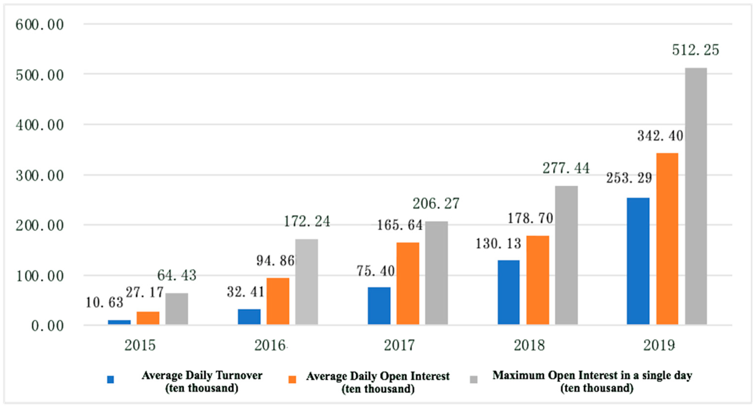
Figure 1 shows the trend of changes in average daily trading volume, average daily open interest, and maximum open interest in a single day for SSE 50ETF index options from 2015 to 2019. We find that the three indicators increase year by year, indicating that the market is developing continuously for the better.

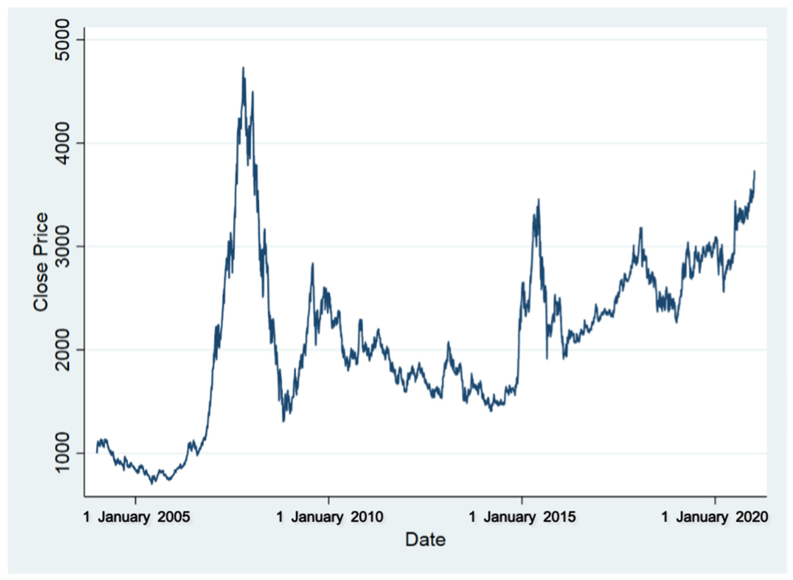
Figure 2 shows the time-series of the daily closing price of the SSE 50 index from 2005 to 2020. The figure shows the market broke through 3500 after a rapid rise from 2006 to 2007 and fell rapidly in 2008. In the following ten years, it rose slowly and fluctuated between 1000 and 3000, and finally reached about 3000 at the end of 2019. The index’s fluctuation has a particular time-varying nature, making it challenging to find a suitable model to describe the volatility.

Table 1. Descriptive statistics.

	Mean	Std. Dev	Min	25%	Median	75%	Max
SSE50	0.0304	0.0155	0.0082	0.0195	0.0264	0.0364	0.0830
N225	0.0255	0.0142	0.0081	0.0170	0.0227	0.0294	0.1383
FCHI	0.0236	0.0132	0.0075	0.0150	0.0205	0.0284	0.1076
STI	0.0181	0.0115	0.0059	0.0110	0.0147	0.0202	0.0924
HSI	0.0247	0.0150	0.0085	0.0164	0.0204	0.0269	0.1394
BVSP	0.0301	0.0145	0.0120	0.0218	0.0268	0.0341	0.1401
GDAXI	0.0233	0.0123	0.0078	0.0152	0.0209	0.0267	0.1023
TWII	0.0197	0.0102	0.0068	0.0128	0.0168	0.0228	0.0616
GSPTSE	0.0172	0.0123	0.0050	0.0101	0.0140	0.0193	0.1030
SPX	0.0191	0.0136	0.0049	0.0108	0.0149	0.0225	0.1049
FTSE	0.0193	0.0117	0.0053	0.0123	0.0166	0.0225	0.1011
HSCCI	0.0288	0.0159	0.0115	0.0193	0.0248	0.0323	0.1360
HSCEI	0.0315	0.0186	0.0116	0.0209	0.0255	0.0359	0.1673
KS11	0.0205	0.0123	0.0075	0.0132	0.0173	0.0232	0.1086
AS51	0.0184	0.0098	0.0061	0.0121	0.0161	0.0215	0.0786
M1	0.1217	0.0768	−0.0065	0.0594	0.1143	0.1736	0.3818
M2	0.1377	0.0466	0.0616	0.0993	0.1375	0.1629	0.2919
CPI	2.6162	1.9233	−1.8100	1.5375	2.1250	3.1900	8.7400

The stock index volatility is calculated by multiplying the standard deviation of the monthly return rate by the square root of the number of trading days in a month; macroeconomic indicators are calculated based on year-on-year growth rate.

is the descriptive statistics of the main variables. Table 1 shows that the SSE 50 index’s daily return is among the best in major international market indexes during the sample period. Meanwhile, compared with other major global market indexes, the standard deviation of daily returns during the sample period of the SSE 50 index is also at a relatively high level, which proves that the SSE 50 is an index with relatively large volatility. However, compared with major domestic macroeconomic indicators, M1, M2, and CPI, the daily return and volatility of the SSE 50 index are relatively small.

4. Empirical Results

According to the research method in the third part, we conduct an empirical analysis of panel data evaluation methods on the introduction of SSE 50ETF index options. Our data range divides the data into two time periods: the pre-option introduction stage: March 2005 to February 2015 and the post-option introduction stage: March 2015 to June

First, we use the data before introducing options to model Equation (4) to construct a counterfactual for the SSE 50 index. The regression’s dependent variable is the monthly volatility of the SSE 50 index. The explanatory variables are the monthly volatility of all international financial market indexes and the growth rate of China’s leading domestic macroeconomic indicators.

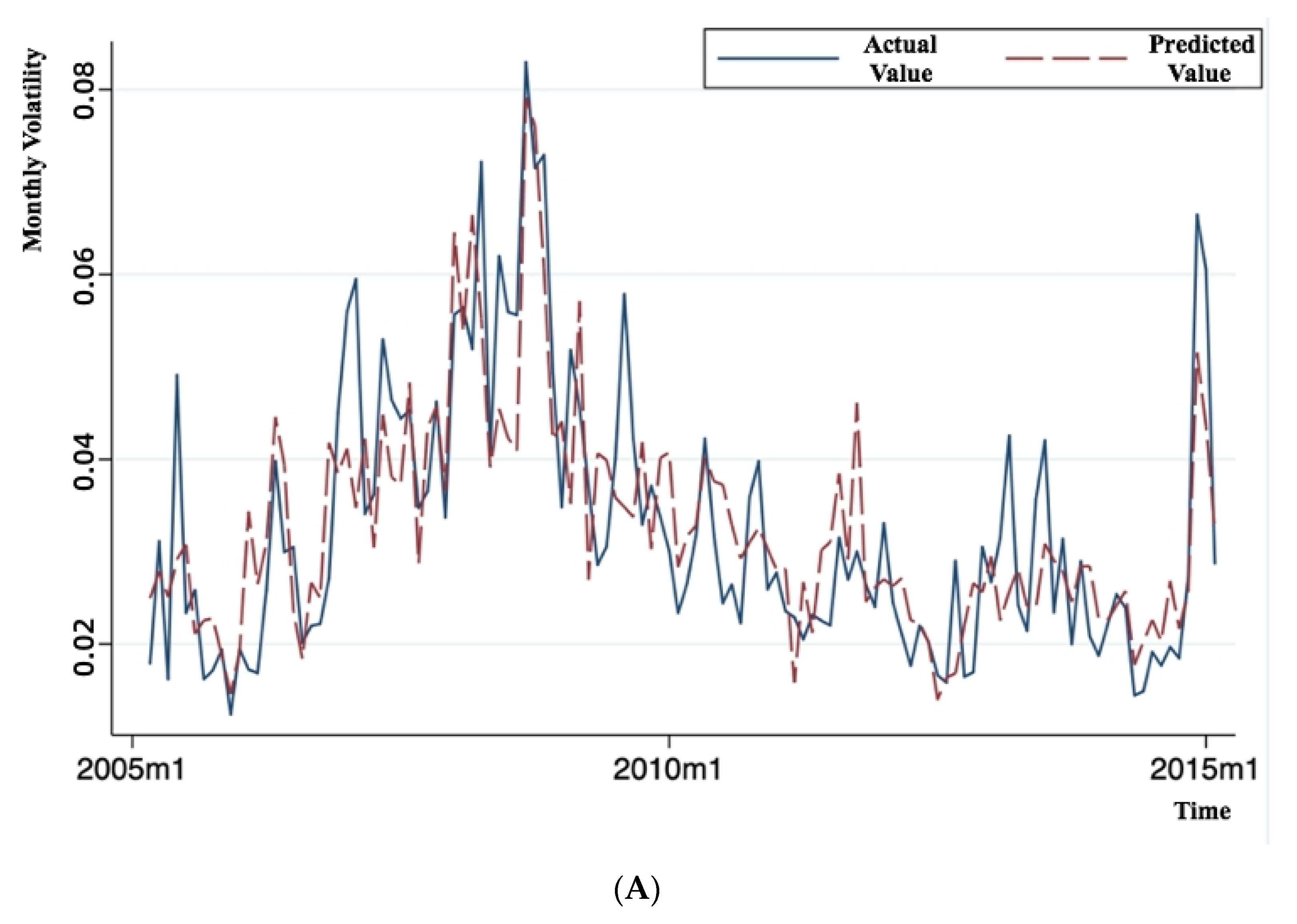
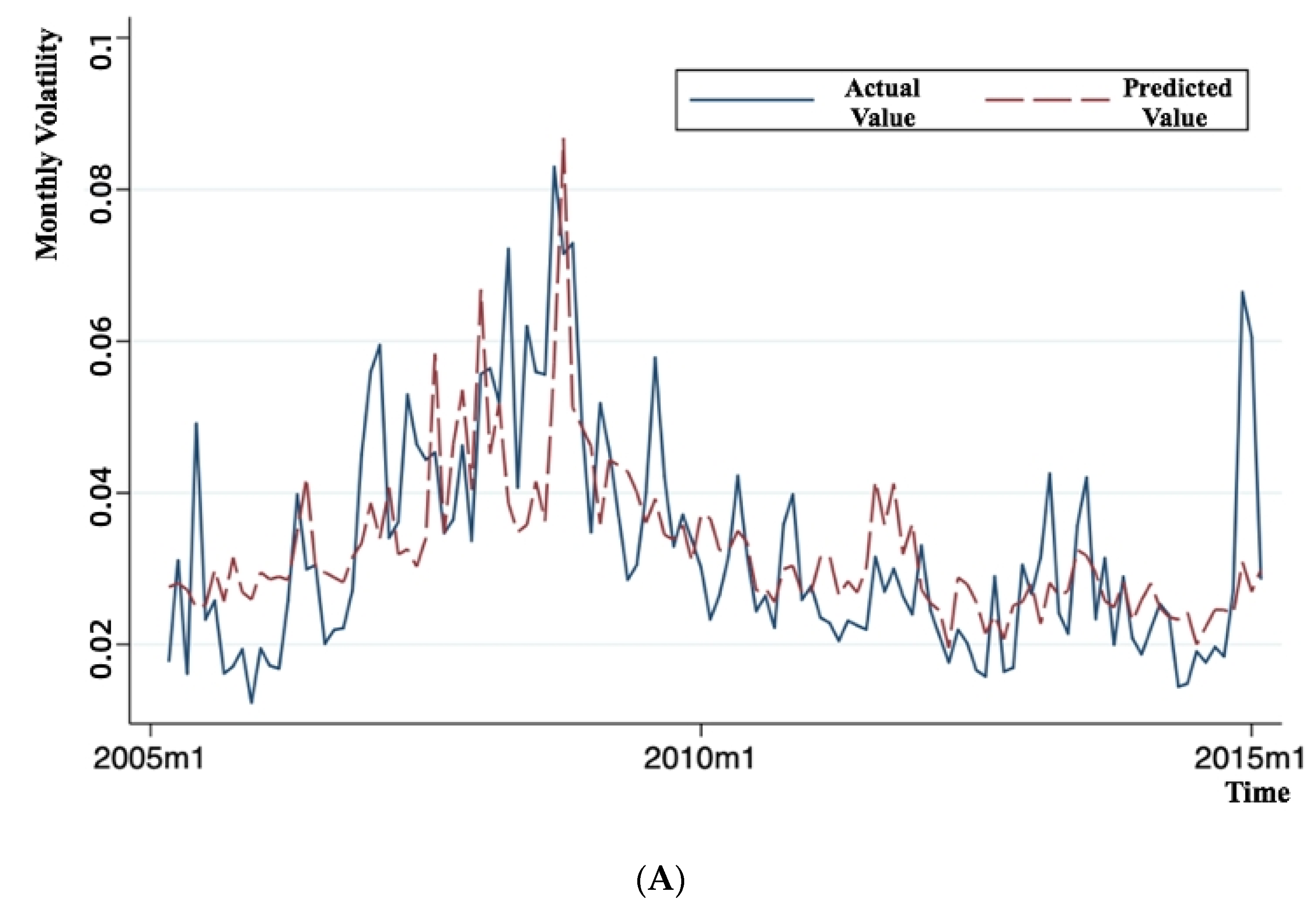
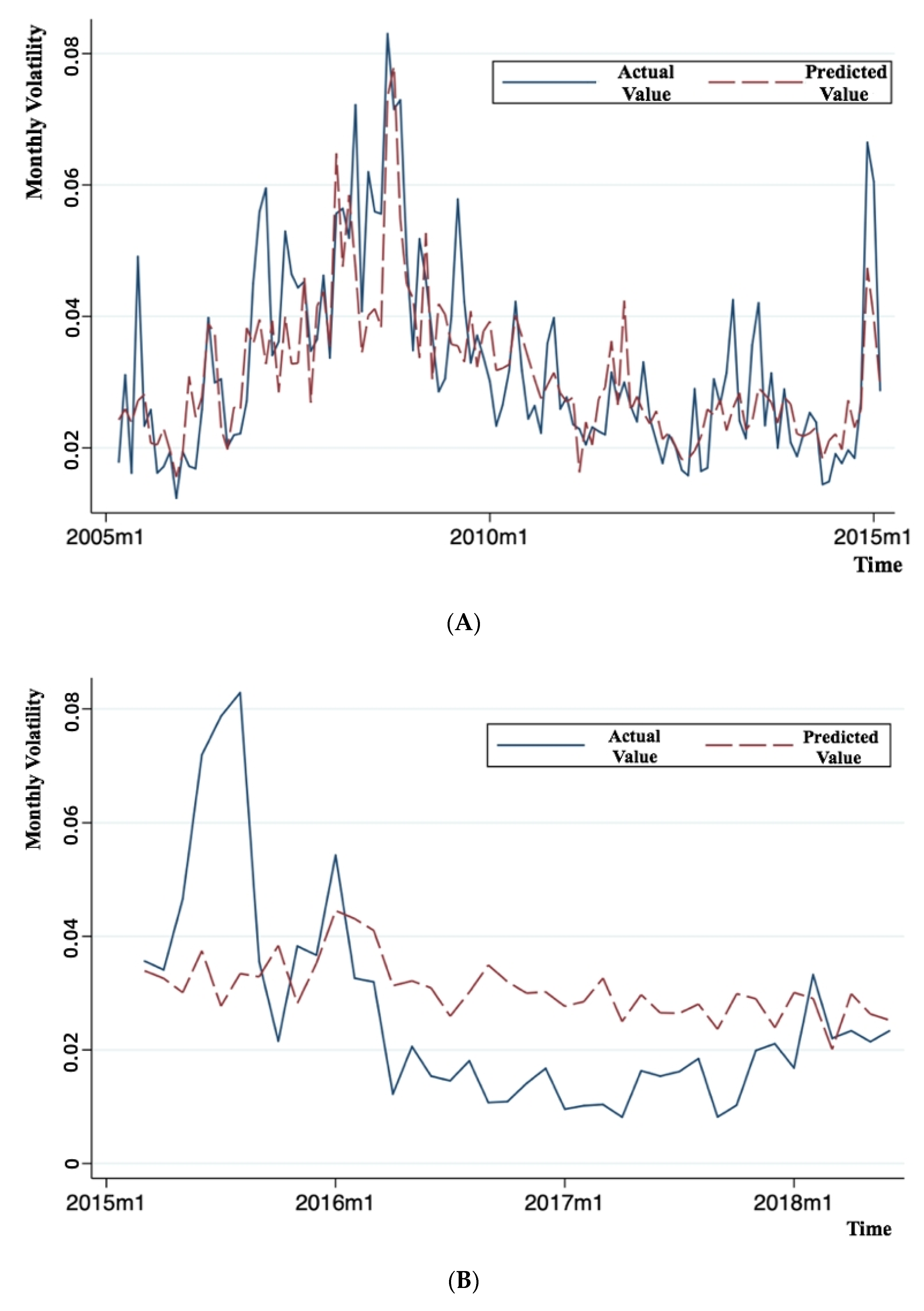
Figure 3 shows the predicted and actual volatility of the SSE 50 index. Panel A of Figure 3 shows that before introducing the SSE 50ETF index option (between 2005 and 2015), the model’s predicted value of the SSE 50 index’s monthly volatility is close to the actual value.

The estimation results are reports in

Table A1. Parameter estimates from OLS regression for counterfactual volatility.

	Parameter	Std. Dev.	t Statistics
Constant	0.017	0.007	2.380
N225	−0.181	0.105	−1.720
FCHI	−0.774	0.321	−2.410
STI	0.089	0.155	0.570
HSI	−1.033	0.304	−3.390
BVSP	0.050	0.143	0.350
GDAXI	0.284	0.276	1.030
TWII	−0.099	0.191	−0.520
GSPTSE	0.291	0.270	1.080
SPX	0.209	0.234	0.890
FTSE	0.892	0.378	2.360
HSCCI	0.116	0.210	0.550
HSCEI	1.094	0.231	4.740
KS11	−0.793	0.181	−4.390
AS51	0.210	0.291	0.720
M1	0.036	0.019	1.880
M2	−0.013	0.042	−0.310
CPI	0.000	0.001	0.600

. Table A1 shows that the t-statistic of 5 out of 17 explanatory variables are above 2, significant at the 5% level. For example, the t-statistic of HSCEI is 4.740, which is greater than the critical value at the 5% level, thereby proving the significance of the explanatory variable HSCEI. Therefore, we find that the SSE 50 index’s monthly volatility can be well predicted by the international financial market indices and domestic macroeconomic indicators before the introduction of SSE 50ETF index options.

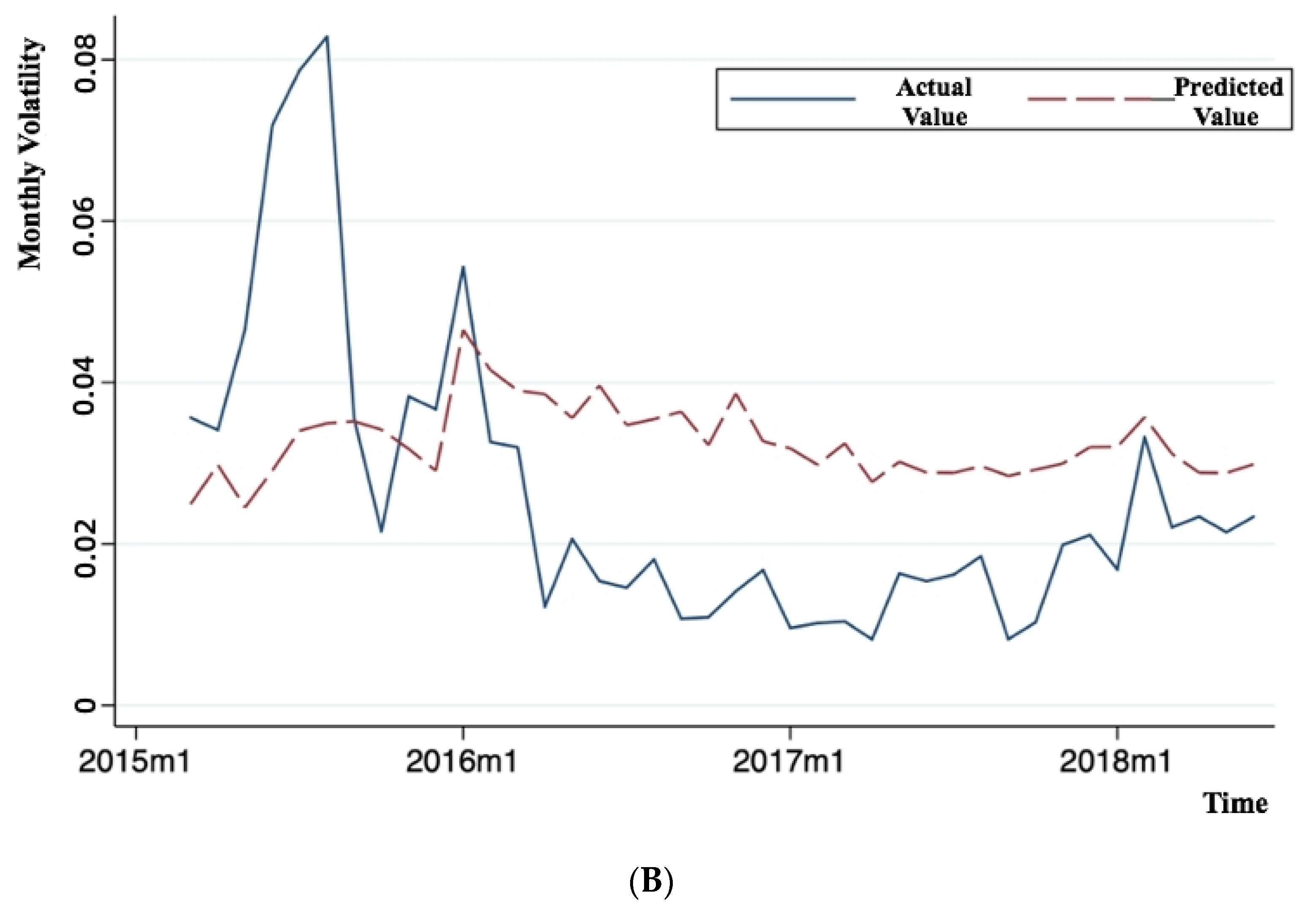
Panel B of Figure 3 presents the predicted and actual monthly volatility of the SSE 50 index after introducing the index options. We find that at the initial stage of option introduction (March 2015–January 2016) the result shows a positive treatment effect. It shows that reducing the spot market’s volatility is not apparent when options were introduced or even when increasing the volatility. The possible reason is that at the beginning of the introduction of SSE 50ETF index options, the various mechanisms were not perfect enough, investors’ understanding of option products was not deep enough, and the information transmission mechanism was not smooth enough, which resulted in investors tending to have a relatively large reaction to negative news. The results show a significant negative treatment effect in the medium and long-term stage after introducing options (February 2016–June 2018), indicating that from a medium and long-term perspective, the introduction of SSE 50ETF index options can reduce the volatility of the spot market. The possible reason is that with the improvement of the options market’s influence mechanism on the spot market and the perfection of its price discovery mechanism, this negative treatment effect appears.

Table 2. Monthly treatment effect based on panel data evaluation approach.

Date	Actual	Predicted	Treatment	Date	Actual	Predicted	Treatment
March 2015	0.0356	0.0405	−0.0049	December 2016	0.0167	0.0309	−0.0141
April 2015	0.0341	0.0366	−0.0025	January 2017	0.0096	0.0282	−0.0186
May 2015	0.0466	0.0335	0.0131	February 2017	0.0102	0.0281	−0.0179
June 2015	0.0719	0.0405	0.0314	March 2017	0.0104	0.0337	−0.0233
July 2015	0.0787	0.0265	0.0522	April 2017	0.0082	0.0237	−0.0156
August 2015	0.0829	0.0369	0.0459	May 2017	0.0163	0.0279	−0.0115
September 2015	0.0355	0.0355	0.0000	June 2017	0.0154	0.0257	−0.0103
October 2015	0.0216	0.0405	−0.0189	July 2017	0.0162	0.0263	−0.0101
November 2015	0.0383	0.0264	0.0119	August 2017	0.0185	0.0291	−0.0106
December 2015	0.0367	0.0398	−0.0031	September 2017	0.0082	0.0249	−0.0167
January 2016	0.0543	0.0476	0.0067	October 2017	0.0103	0.0304	−0.0201
February 2016	0.0326	0.0470	−0.0144	November 2017	0.0199	0.0305	−0.0106
March 2016	0.0320	0.0434	−0.0114	December 2017	0.0211	0.0224	−0.0013
April 2016	0.0122	0.0301	−0.0178	January 2018	0.0168	0.0311	−0.0142
May 2016	0.0206	0.0320	−0.0114	February 2018	0.0332	0.0282	0.0050
June 2016	0.0154	0.0305	−0.0151	March 2018	0.0220	0.0206	0.0015
July 2016	0.0146	0.0243	−0.0097	April 2018	0.0234	0.0334	−0.0100
August 2016	0.0181	0.0299	−0.0118	May 2018	0.0215	0.0288	−0.0074
September 2016	0.0107	0.0355	−0.0248	June 2018	0.0234	0.0259	−0.0025
October 2016	0.0109	0.0334	−0.0224
November 2016	0.0141	0.0285	−0.0144
Mean	0.0342	0.0352	−0.0057
Std. Dev	0.0220	0.0066	0.0169
t-statistics	9.84	13.22	3.23

The treatment effect is the difference between the actual and the predicted volatility, and the Newey–West robust t-statistic is reported.

reports the estimated treatment effect following the introduction of SSE 50ETF index options. The mean is −0.0057 with a t-statistic of 3.23, which is significant at the 5% level. The result indicates that the introduction of index options can indeed reduce the volatility of the spot market. The magnitude is equivalent to a 21% reduction in stock market volatility over three years. However, at the beginning of options trading, this effect was not pronounced. This result can also explain to a certain extent that the introduction of SSE 50ETF index options has a time-lag effect on the spot market. That is, reducing volatility in the short term—approximately half a year—is not apparent. The results are consistent with Yang et al. (2012), who found that China’s index futures market’s price discovery function was not sizeable when it was first introduced. Over time, more and more institutional investors enter the market, leading to the continuous improvement of the market’s price discovery function and effectively reducing stock market volatility.

To test whether the introduction of SSE 50ETF index options has a long-term treatment effect, we construct an ARMA model formulated in Equation (9). Specifically, we build the AR (1) model based on the AIC and BIC as follows:

$${\widehat{\Delta }}_{1t}=0.011+0.796{\widehat{\Delta }}_{1,t-1}+{\widehat{\eta }}_t.$$

(14)

The t-statistics of the treatment effect with first-order lag is 3.23, significant at the 1% level.

4.1. Robustness Checks

4.1.1. Principal Component Analysis

Given many explanatory variables, we performed principal component analysis on these 16 variables to extract the principal components. After that, the principal components were used as an independent variable to construct the counterfactual volatility to analyze the treatment effect after introducing SSE 50 index options.

Table A2. Construction of principal components.

Principal Components	Eigenvalues	Distinction	Proportion	Cumulative Ratio
PC 1	11.99	10.225	0.749	0.749
PC 2	1.765	1.238	0.11	0.86
PC 3	0.527	0.138	0.033	0.893
PC 4	0.389	0.11	0.024	0.917
PC 5	0.279	0.057	0.017	0.934

reports the first five principal components. We find that the first four principal components can explain 91.7% of the prediction variance, so we choose the first four principal components to model Equations (4) and (6). Similar to the panel data evaluation approach, we divide the sample into the pre-option and post-option stages and predict counterfactual volatility following the introduction of SSE 50 index options. Panel A of Figure 4 shows the predicted and actual monthly volatility of the SSE 50 index before introducing index options.

Panel B of Figure 4 reports the actual and predicted value of the SSE 50 index’s monthly volatility after introducing SSE 50ETF index options. Shortly after the index options were introduced, the volatility of the SSE 50 index witnesses a short-term increase. One year after the introduction, the index volatility shows a significant decrease. These results validate the robustness of the panel data evaluation approach.

Table 3. Monthly treatment effect based on principal component analysis.

Date	Actual	Predicted	Treatment	Date	Actual	Predicted	Treatment
March 2015	0.0356	0.0249	0.0107	December 2016	0.0167	0.0327	−0.0160
April 2015	0.0341	0.0298	0.0043	January 2017	0.0096	0.0318	−0.0223
May 2015	0.0466	0.0245	0.0221	February 2017	0.0102	0.0298	−0.0196
June 2015	0.0719	0.0291	0.0428	March 2017	0.0104	0.0325	−0.0221
July 2015	0.0787	0.0340	0.0447	April 2017	0.0082	0.0277	−0.0195
August 2015	0.0829	0.0349	0.0479	May 2017	0.0163	0.0302	−0.0138
September 2015	0.0355	0.0352	0.0004	June 2017	0.0154	0.0288	−0.0135
October 2015	0.0216	0.0342	−0.0126	July 2017	0.0162	0.0288	−0.0126
November 2015	0.0383	0.0318	0.0065	August 2017	0.0185	0.0296	−0.0112
December 2015	0.0367	0.0290	0.0076	September 2017	0.0082	0.0284	−0.0202
January 2016	0.0543	0.0465	0.0078	October 2017	0.0103	0.0292	−0.0189
February 2016	0.0326	0.0415	−0.0089	November 2017	0.0199	0.0300	−0.0101
March 2016	0.0320	0.0390	−0.0070	December 2017	0.0211	0.0320	−0.0109
April 2016	0.0122	0.0385	−0.0263	January 2018	0.0168	0.0320	−0.0152
May 2016	0.0206	0.0356	−0.0150	February 2018	0.0332	0.0357	−0.0025
June 2016	0.0154	0.0396	−0.0243	March 2018	0.0220	0.0312	−0.0091
July 2016	0.0146	0.0347	−0.0202	April 2018	0.0234	0.0288	−0.0054
August 2016	0.0181	0.0355	−0.0174	May 2018	0.0215	0.0288	−0.0073
September 2016	0.0107	0.0364	−0.0257	June 2018	0.0234	0.0299	−0.0065
October 2016	0.0109	0.0322	−0.0213
November 2016	0.0141	0.0386	−0.0245
Mean	0.0260	0.0326	−0.0066
Std. Dev	0.0186	0.0045	0.0186
t-statistics	11.34	15.29	4.89

The treatment effect is the difference between the actual and the predicted volatility, and the Newey–West robust t-statistic is reported.

reports the treatment effect estimated from the principal component method. We find that the mean of the treatment effect is −0.0066 with a t-statistic of 4.89, which is significant at the 5% level. The results indicate that our findings are similar to that of the panel data evaluation approach.

4.1.2. GARCH Model

Some existing studies use the GARCH model with a dummy variable designed to detect the volatility changes after the introduction of the futures contract. This approach relies on a time-series comparison of estimated unconditional or conditional volatility before and after the policy shock. We argue that this approach is subject to uncontrolled market factors or structural changes that affect market volatility (Bhattacharya et al. 1986; Bologna and Cavallo 2002), resulting in an omitted variable bias.

Although the GARCH model is susceptible to selecting different periods and cannot provide a good explanation of the causal relationship between the policy or product launch and the dependent variable, the model itself can still reflect some properties of the volatility changes in a certain period. To further verify whether the SSE 50 index volatility has relatively different treatment effects in the short term, midterm, and long term, we consider using the GARCH model to add dummy variables for modeling and analysis.

First, to increase the number of samples, we use the daily yield data of the SSE 50 index. Next, to study the fluctuations in different periods, we introduce dummy variables $D_{1t}$ and $D_{2t}$. The specific values are as follows:

$$D_{1t}=\{\begin{array}{cc}0& \hfill \mathrm{Before\; the\; option\; is\; listed} \left(\mathrm{2013.2.8}—\mathrm{2015.2.8}\right)\\ 1& \hfill \mathrm{After\; the\; option\; is\; listed} \left(\mathrm{2015.2.9}—\mathrm{2019.2.8}\right)\end{array}$$

(15)

$$D_{2t}=\{\begin{array}{lll}0& \hfill \mathrm{Before\; the\; option\; is\; listed}& \left(\mathrm{2013.2.8}—\mathrm{2015.2.8}\right)\\ 0& \hfill \mathrm{The\; first\; year\; after\; the\; option\; is\; listed}& \left(\mathrm{2015.2.9}—\mathrm{2016.2.8}\right)\\ 1& \hfill \mathrm{After\; the\; first\; year\; of\; the\; option’s\; listing}& \left(\mathrm{2016.2.9}—\mathrm{2019.2.8}\right)\end{array}$$

(16)

By adding dummy variables to the model, we can better observe volatility changes in different periods after listing. The model we established and the results of the model are as follows:

$${\sigma }_t^2={\alpha }_0+{\alpha }_1{\epsilon }^2{}_{t-1}+{\beta }_1{\sigma }^2{}_{t-1}+{\gamma }_1{D}_{1t}+{\gamma }_2{D}_{2t}.$$

(17)

The results are presented in

Table 4. GARCH (1, 1) model estimation.

Model		Parameter
ARMA	Constant	0.0006 **
		(0.0003)
	AR:
	L.2	−0.7078 ***
		(0.0050)
	L.3	−0.5252 ***
		(0.0050)
	MA:
	L.2	0.7047 ***
		(0.0010)
	L.3	0.5407 ***
		(0.0012)
GARCH	Constant	−12.2148 ***
		(0.2363)
	D1	1.2436 ***
		(0.2476)
	D2	−2.1733 **
		(0.2385)
	ARCH:
	L.1	0.0772 ***
		(0.0079)
	GARCH:
	L.1	0.9031 ***
		(0.0087)
Log-likelihood	4273.666
Wald chi2	1520 ***

The robust standard errors are reported in the parentheses; *, **, and *** denote significance at the 10%, 5%, and 1% levels, respectively.

. We find that ${\alpha }_1=0.0772$ and ${\beta }_1=0.9031$, which are both significant at the 1% significance level, and ${\alpha }_1+{\beta }_1=0.98<1$, which satisfies stationary conditions. At the same time, the coefficient ${\gamma }_1$ of the dummy variable $D_{1t}$ is equal to 1.2436, which is positive and significant at the 1% level, indicating that SSE 50ETF index options’ volatility increases in the short term after introduction. Moreover, the coefficient ${\gamma }_2$ of the dummy variable $D_{2t}$ amounts to −2.1733, which is negative and significant at the 1% level, suggesting that the SSE 50ETF index option has a negative effect on the volatility of the SSE 50 index in the long run. Furthermore, ${\gamma }_1+{\gamma }_2=-0.93<0$, which indicates that in the long run, after the introduction of the SSE 50ETF index option, the volatility of the SSE 50 index reduced significantly. The findings are consistent with the preliminary results obtained from the panel data evaluation approach.

4.1.3. LASSO Regression

Similar to the principal component analysis method, we can also regard the screening of the control group (independent variables) as a data screening for high-dimensional variables. Specifically, the LASSO method can be used to screen independent variables. According to the method proposed by Li and Bell (2017), in the general linear model fitting results, the deviation of the model is usually small, but it produces a large variance, which may result in model overfitting. Machine learning methods such as LASSO, by contrast, can reduce the variance of the prediction model by adding some constraints to the model, thereby achieving a better forecast effect.

First, the general linear regression model is formulated as follows:

$$y_{1t}=x_t^{\prime }\beta +v_{1t}, t=1,\dots ,T_1.$$

(18)

The LASSO method minimizes the following formula by selecting the appropriate $\beta$:

$${\displaystyle \sum }_{t=1}^{T_1}{\left[y_{1t}-x_t^{\prime }\beta \right]}^2+\lambda {\displaystyle \sum }_{j=1}^N\left|{\beta }_j\right|,$$

(19)

where $\lambda$ denotes the adjustment parameter and $\lambda \ge 0$. $\lambda$ can be used to control the adjustment intensity of the non-zero parameter ${\beta }_j$. When $\lambda =0$, the model reduces to an ordinary linear regression; when $\lambda =\infty$, all parameters ${\beta }_j$ shrink to zero. We use the $k$-fold cross-validation method in the choice of $\lambda$.

Table A3. Parameter estimates from LASSO and OLS regression.

	LASSO	OLS
Constant	−0.151	−0.186
N225	−0.311	−0.548
FCHI	0.085	0.112
STI	−0.551	−0.921
HIS	0.099	0.048
BVSP	−0.041	−0.127
TWII	0.310	0.333
GSPTSE	0.077	0.191
SPX	0.483	0.814
FTSE	0.819	1.085
HSCEI	−0.619	−0.718
KS11	0.192	0.268
AS51	0.040	0.035
M1	−0.024	−0.013
M2	0.000	0.000
CPI	0.017	0.018

reports the parameter estimates of the LASSO and OLS. The result shows that after screening with the LASSO method, the model eliminates the two variables GDAXI and HSCCI and compares the coefficients obtained by the LASSO and OLS.

The actual and predicted value of the SSE 50 index’s monthly volatility in and out of the sample is shown in Figure 5. When index options were introduced, the volatility of the SSE 50 index experienced a short-term increase. One year after the introduction, starting in 2016, the index volatility shows a significant decrease.

Table 5. Treatment effect from LASSO regression.

Date	Actual	Predicted	Treatment	Date	Actual	Predicted	Treatment
March 2015	0.0356	0.0339	0.0017	December 2016	0.0167	0.0302	−0.0135
April 2015	0.0341	0.0326	0.0015	January 2017	0.0096	0.0277	−0.0181
May 2015	0.0466	0.0301	0.0165	February 2017	0.0102	0.0285	−0.0183
June 2015	0.0719	0.0375	0.0344	March 2017	0.0104	0.0326	−0.0223
July 2015	0.0787	0.0277	0.0510	April 2017	0.0082	0.0250	−0.0169
August 2015	0.0829	0.0334	0.0494	May 2017	0.0163	0.0297	−0.0134
September 2015	0.0355	0.0329	0.0027	June 2017	0.0154	0.0265	−0.0112
October 2015	0.0216	0.0384	−0.0168	July 2017	0.0162	0.0265	−0.0103
November 2015	0.0383	0.0282	0.0101	August 2017	0.0185	0.0281	−0.0096
December 2015	0.0367	0.0353	0.0014	September 2017	0.0082	0.0236	−0.0155
January 2016	0.0543	0.0445	0.0098	October 2017	0.0103	0.0299	−0.0196
February 2016	0.0326	0.0431	−0.0105	November 2017	0.0199	0.0290	−0.0091
March 2016	0.0320	0.0410	−0.0091	December 2017	0.0211	0.0239	−0.0028
April 2016	0.0122	0.0313	−0.0191	January 2018	0.0168	0.0301	−0.0133
May 2016	0.0206	0.0322	−0.0116	February 2018	0.0332	0.0291	0.0042
June 2016	0.0154	0.0309	−0.0155	March 2018	0.0220	0.0201	0.0019
July 2016	0.0146	0.0259	−0.0114	April 2018	0.0234	0.0299	−0.0065
August 2016	0.0181	0.0302	−0.0121	May 2018	0.0215	0.0263	−0.0049
September 2016	0.0107	0.0349	−0.0242	June 2018	0.0234	0.0252	−0.0019
October 2016	0.0109	0.0320	−0.0211
November 2016	0.0141	0.0300	−0.0159
Mean	0.0169	0.0275	−0.0106
Std. Dev	0.0065	0.0030	0.0074
t-statistics	5.32	4.33	6.23

The treatment effect is the difference between the actual and predicted volatility, and the Newey–West robust t-statistic is reported.

reports the treatment effect of the LASSO method. We find that the mean value of treatment effect with the LASSO method is −0.0106 with a t-statistic of 6.23, significant at the 5% level. The result suggests that our primary findings remain robust with LASSO regression.

4.1.4. Falsification Test

In this section, we conduct the final robustness check by further discussing the validity of our model. We can only use the data from the period before introducing the SSE 50 index options for analysis and construct counterfactual volatility for the SSE 50 index to verify that the results of the treatment effect obtained by the panel data evaluation method at this stage are not significant. Furthermore, we find that the introduction of SSE 50ETF index options does lead to a decrease in the SSE 50 index volatility.

To conduct the falsification test, we choose one year before (February 2014) introducing the SSE 50ETF index options as the artificial event date and estimate treatment effect following the similar strategy as outlined in the methodology section. We use the pre-event period to evaluate the model parameters and obtain predicted counterfactual volatility for the SSE 50 index in the post-event period.

Table 6. Falsification test.

Date	Actual	Predicted	Treatment
March 2014	0.0254	0.0231	0.0022
April 2014	0.0239	0.0259	−0.0020
May 2014	0.0144	0.0199	−0.0055
June 2014	0.0149	0.0222	−0.0073
July 2014	0.0191	0.0215	−0.0024
August 2014	0.0177	0.0188	−0.0012
September 2014	0.0197	0.0269	−0.0072
October 2014	0.0184	0.0210	−0.0025
November 2014	0.0272	0.0227	0.0045
December 2014	0.0665	0.0442	0.0223
January 2015	0.0605	0.0367	0.0239
February 2015	0.0287	0.0350	−0.0062
Mean	0.0280	0.0265	0.0015
Std. Dev	0.0172	0.0079	0.0107
t-statistics	8.36	6.39	0.48

The treatment effect is the difference between the actual and predicted volatility, and the Newey–West robust t-statistic is reported.

reports the results. We find that using the artificial date of introduction of 50 index options, the average value of the monthly treatment effect is 0.0280 with a t-statistic of 0.48, which is insignificant at the conventional level. Therefore, we find that the treatment effect becomes insignificant in the falsification test, in which one year before the actual date of introduction is set to be the event date. The results provide support to the validity of our primary empirical model.

4.2. Discussion

From the above empirical analysis, we find that the short-term impact on the SSE 50 index’s volatility is not significant in the short term following the introduction of SSE 50 index options. There are insignificant changes in the volatility of the equity market from March 2015 to January 2016. The findings of insignificant short-term effect differ from Chen et al. (2013), which find a significant effect of CSI 300 index futures trading shortly after its introduction in China. The treatment effect of index options trading emerges after February 2016. We propose possible explanations for this phenomenon according to the specific circumstances of option listing and the stock market trend at that time.

First of all, the dramatic stock market crash occurred in June 2015, shortly after the index option was introduced. The stock market crash is a significant event that directly led to a sharp increase in the SSE 50 index returns’ volatility from an average of 0.03 to 0.07 from June to August 2015. The stock market did not return to normal until the end of 2015. Consistent with our empirical results, we find that the effect of SSE 50ETF index options on the volatility of the SSE 50 index is statistically significant in the long run after 2016. The result implies that aggregate market fears, especially during stock market crashes, tend to subsume the effect of index options trading.

Secondly, based on SSE 50ETF index options’ trading volume, the current average daily trading volume, average daily open interest, and maximum single-day open interest have increased by more than three times compared with those in 2015. The findings are consistent with the view that the increase in trading volume following the introduction of index options facilitates price discovery in the stock market and further reduces index returns volatility. The improved price discovery helps disseminate information and increase news speed to be incorporated into asset prices.

Finally, the Shanghai Stock Exchange has optimized the calculation method of the settlement price of inactive options contracts and strengthened the management of option holding limits since 1 January 2016 to improve the transparency of options transactions. It contributes to the options market’s operation and plays a positive role in reducing the stock index volatility. Thus, the insignificant short-term effect may be due to a lack of information transparency during the early stage of index options trading.

5. Conclusions

This study uses different financial market index data and major macroeconomic indicators as panel data to conduct an empirical analysis on the introduction of SSE 50ETF index options and finds that the introduction of SSE 50ETF index options can reduce the volatility of the SSE 50 index. The study shows that the panel data policy evaluation approach is very suitable for analyzing the impact of a particular policy or product launch. It can well avoid the omission of certain error variables due to uncontrollable market factors. Moreover, an investigation of the impact of futures trading on the Chinese stock market can enrich the current literature and verify the robustness of previous findings across countries. Specially, this paper has examined the robustness of Fleming et al.’s (1996) and Jong and Donders’s (1998) findings that index options contribute to the price discovery process involving index securities through information sharing, and that an index option has a higher informational role relative to an index.

We find that the introduction of SSE 50ETF index options has not caused significant changes in the volatility of the SSE 50 index in the short term due to the immaturity of the market and the impact of the 2015 Chinese stock market crash. However, index options trading has significantly reduced the volatility of the equity market over the long run. The findings suggest that the introduction of index options can improve the Chinese stock market’s liquidity and price discovery efficiency, thus providing investors with more risk management and investment tools. We also use the principal component analysis, GARCH model, and LASSO regression and reach similar conclusions, suggesting that our findings are robust to alternative prediction methods and falsification tests.

Our findings provide several important policy implications to regulatory agencies and general investors. On the one hand, more derivative products should be introduced to the Chinese financial markets to increase market completeness and dampen volatilities, which reduce the likelihood of stock market crashes. On the other hand, investors benefit from trading index options in terms of risk management, and such trading activities are helpful to lower systematic risk in the financial market.

This paper constructs counterfactual volatilities through the linear model. Although the prediction accuracy is satisfactory, nonlinear models can be considered in future research to further improve the prediction accuracy of counterfactual volatiles and make the main finding more robust.

References

- Ahn, Kwangwon, Yingyao Bi, and Sungbin Sohn. 2019. Price discovery among SSE 50 Index-based spot, futures, and options markets. Journal of Futures Markets 39: 238–59. [Google Scholar]
- Anderson, Heather M., and Farshid Vahid. 2007. Forecasting the volatility of Australian stock returns. Journal of Business and Economic Statistics 25: 76–90. [Google Scholar]
- Antoniou, Antonios, Gregory Koutmos, and Andreas Pericli. 2005. Index futures and positive feedback trading: Evidence from major stock exchanges. Journal of Empirical Finance 12: 219–38. [Google Scholar]
- Arkorful, Gideon Bruce, Haiqiang Chen, Xiaoqun Liu, and Chuanhai Zhang. 2020. The impact of options introduction on the volatility of the underlying equities: Evidence from the Chinese stock markets. Quantitative Finance 20: 2015–24. [Google Scholar]
- Bai, ChongEn, Qi Li, and Min Ouyang. 2014. Property taxes and home prices: A tale of two cities. Journal of Econometrics 180: 1–15. [Google Scholar]
- Bhattacharya, Anand K., Anju Ramjee, and Balasubramani Ramjee. 1986. The causal relationship between futures price volatility and the cash price volatility of GNMA securities. Journal of Futures Markets 6: 29–39. [Google Scholar]
- Bohl, Martin T., Christian A. Salm, and Bernd Wilfling. 2011. Do individual index futures investors destabilize the underlying spot market? Journal of Futures Markets 31: 81–101. [Google Scholar]
- Bologna, Pierluigi, and Laura Cavallo. 2002. Does the introduction of stock index futures effectively reduce stock market volatility? Is the ‘futures effect’ immediate? Evidence from the Italian stock exchange using GARCH. Applied Financial Economics 12: 183–92. [Google Scholar]
- Chen, Haiqiang, Qian Han, Yingxing Li, and Kai Wu. 2013. Does Index Futures Trading Reduce Volatility in the Chinese Stock Market? A Panel Data Evaluation Approach. Journal of Futures Markets 33: 1167–90. [Google Scholar]
- Corgel, John B., and Gerald D. Gay. 1984. The impact of gnma futures trading on cash market volatility. Real Estate Economics 12: 176–90. [Google Scholar]
- Darrat, Ali F., and Shafiqur Rahman. 1995. Has futures trading activity caused stock price volatility? Journal of Futures Markets 15: 537–57. [Google Scholar]
- Du, Zaichao, and Lin Zhang. 2015. Home-purchase restriction, property tax and housing price in China: A counterfactual analysis. Journal of Econometrics 188: 558–68. [Google Scholar]
- Engle, Robert F., and Juri Marcucci. 2006. A long-run pure variance common features model for the common volatilities of the Dow Jones. Journal of Econometrics 132: 7–42. [Google Scholar]
- Figlewski, Stephen. 1981. Futures trading and volatility in the GNMA market. Journal of Finance 36: 445–56. [Google Scholar]
- Fleming, Jeff, Barbara Ostdiek, and Robert E. Whaley. 1996. Trading costs and the relative rates of price discovery in stock, futures, and option markets. The Journal of Futures Markets 16: 353. [Google Scholar]
- Gao, Yang, and Bianxia Sun. 2018. Impacts of introducing index futures on stock market volatilities: New evidences from China. Review of Pacific Basin Financial Markets and Policies 21: 1850024. [Google Scholar]
- He, Feng, Baiao Liu-Chen, Xiangtong Meng, Xiong Xiong, and Wei Zhang. 2020. Price discovery and spillover dynamics in the Chinese stock index futures market: A natural experiment on trading volume restriction. Quantitative Finance 20: 2067–83. [Google Scholar]
- Hsiao, Cheng, H. Steve Ching, and Shui Ki Wan. 2012. A panel data approach for program evaluation: Measuring the benefits of political and economic integration of Hong Kong with mainland China. Journal of Applied Econometrics 27: 705–40. [Google Scholar]
- Huo, Rui, and Abdullahi D. Ahmed. 2018. Relationships between Chinese stock market and its index futures market: Evaluating the impact of QFII scheme. Research in International Business and Finance 44: 135–52. [Google Scholar]
- Ibrahim, Mansor H., and Hassanuddeen Aziz. 2003. Macroeconomic variables and the Malaysian equity market: A view through rolling subsamples. Journal of Economic Studies 30: 6–27. [Google Scholar]
- Jalan, Akanksha, Roman Matkovskyy, and Andrew Urquhart. 2021. What effect did the introduction of Bitcoin futures have on the Bitcoin spot market? The European Journal of Finance 27: 1251–81. [Google Scholar]
- Jong, Frank De, and Monique WM Donders. 1998. Intraday lead-lag relationships between the futures-, options and stock market. Review of Finance 1: 337–59. [Google Scholar]
- Ke, Xiao, Haiqiang Chen, Yongmiao Hong, and Cheng Hsiao. 2017. Do China’s high-speed-rail projects promote local economy? New evidence from a panel data approach. China Economic Review 44: 203–26. [Google Scholar]
- Kurov, Alexander. 2008. Investor sentiment, trading behavior and informational efficiency in index futures markets. Financial Review 43: 107–27. [Google Scholar]
- Kutan, Ali M., and Haigang Zhou. 2006. Determinants of returns and volatility of Chinese ADRs at NYSE. Journal of Multinational Financial Management 16: 1–15. [Google Scholar]
- Kutan, Ali M., Yukun Shi, Mingzhe Wei, and Yang Zhao. 2018. Does the introduction of index futures stabilize stock markets? Further evidence from emerging markets. International Review of Economics & Finance 57: 183–97. [Google Scholar]
- Li, Jinliang, Yao Lei, and Shujing Li. 2012. Market Depth, Liquidity and volatility: The impact of the launch of Shanghai and Shenzhen 300 stock index futures on the spot market. Journal of Financial Research 6: 124–38. (In Chinese). [Google Scholar]
- Li, Kathleen T., and David R. Bell. 2017. Estimation of average treatment effects with panel data: Asymptotic theory and implementation. Journal of Econometrics 197: 65–75. [Google Scholar]
- Liu, Jinyu, and Rui Zhong. 2018. Equity index futures trading and stock price crash risk: Evidence from Chinese markets. Journal of Futures Markets 38: 1313–33. [Google Scholar]
- Liu, Pangpang. 2017. An empirical analysis of the impact of the options market on the volatility of the spot market: A comparison of SSE 50ETF options before and after listing. Statistics and Information Forum 32: 50–58. (In Chinese). [Google Scholar]
- Nguyen, Anh Thi Kim, and Loc Dong Truong. 2020. The impact of index future introduction on spot market returns and trading volume: Evidence from Ho Chi Minh Stock Exchange. The Journal of Asian Finance, Economics, and Business 7: 51–59. [Google Scholar]
- Osamwonyi, Ifuero Osad, and Esther Ikavbo Evbayiro-Osagie. 2012. The relationship between macroeconomic variables and stock market index in Nigeria. Journal of Economics 3: 55–63. [Google Scholar]
- Ouyang, Min, and Yulei Peng. 2015. The treatment-effect estimation: A case study of the 2008 economic stimulus package of China. Journal of Econometrics 188: 545–57. [Google Scholar]
- Pericli, Andreas, and Gregory Koutmos. 1997. Index futures and options and stock market volatility. Journal of Futures Markets 17: 957–74. [Google Scholar]
- Qiao, Gaoxiu, Qiang Liu, and Maojun Zhang. 2014. The impact of the Shanghai and Shenzhen 300 stock index futures listing on continuous volatility and jump volatility in the spot market. China Management Science 22: 9–18. (In Chinese). [Google Scholar]
- Simpson, Gary, and Timothy C. Ireland. 1982. The effect of futures trading on the price volatility of GNMA securities. Journal of Futures Market 2: 357. [Google Scholar]
- Staikouras, Sotiris K. 2006. Testing the stabilization hypothesis in the UK short-term interest rates: Evidence from a GARCH-X model. Quarterly Review of Economics and Finance 46: 169–89. [Google Scholar]
- Truong, Loc Dong, Anh Thi Kim Nguyen, and Dut Van Vo. 2021. Index future trading and spot market volatility in frontier markets: Evidence from Ho Chi Minh Stock Exchange. Asia-Pacific Financial Markets 28: 353–66. [Google Scholar]
- Wang, Steven S., and Li Jiang. 2004. Location of trade, ownership restrictions, and market illiquidity: Examining Chinese A-and H-shares. Journal of Banking & Finance 28: 1273–97. [Google Scholar]
- Wu, Guowei. 2015. The impact of the launch of stock index options on the volatility of China’s stock market: An empirical analysis based on the high-frequency data of SSE 50ETF index options. China Economic and Trade Guide 14: 37–38. (In Chinese). [Google Scholar]
- Xiong, Xiong, Yu Zhang, Wei Zhang, and Yongjie Zhang. 2011. The impact of the launch of stock index options on the volatility of the stock market and stock index futures markets: Taking KOSPI200 stock index options as an example. System Engineering Theory and Practice 31: 785–91. (In Chinese). [Google Scholar]
- Yang, Jian, Zihui Yang, and Yinggang Zhou. 2012. Intraday price discovery and volatility transmission in stock index and stock index futures markets: Evidence from China. Journal of Futures Markets 32: 99–121. [Google Scholar]
- Zhang, Jing, and Fuyi Song. 2016. The impact of Shanghai stock exchange 50 options on the underlying stock: Perspective of liquidity and volatility. Financial Development Research 3: 59–65. (In Chinese). [Google Scholar]
- Zhang, Linling, Ruyin Long, and Hong Chen. 2019. Do car restriction policies effectively promote the development of public transport? World Development 119: 100–10. [Google Scholar]
- Zhao, Shangmei, Guiping Sun, and Haijun Yang. 2015. Analysis of the volatility of stock options on the stock market: An agent-based computational experimental financial simulation perspective. Chinese Journal of Management Engineering 29: 207–15. (In Chinese). [Google Scholar]