Article

Are GARCH and DCC Values of 10 Cryptocurrencies Affected by COVID-19?

1
Department of Accounting, Finance and Economics, Griffith University, Nathan 4111, Australia
2
Xiamen National Accounting Institute, Xiamen 361005, China
*
Author to whom correspondence should be addressed.
J. Risk Financial Manag. 2022, 15(3), 113; https://doi.org/10.3390/jrfm15030113
Submission received: 11 January 2022 / Revised: 24 February 2022 / Accepted: 28 February 2022 / Published: 1 March 2022
(This article belongs to the Special Issue Emerging Markets)

Abstract

:
This paper examines the dynamic conditional correlations among 10 cryptocurrencies and the possibility of hedging investment strategies among multiple cryptocurrencies over the period affected by COVID-19 from 2017 to 2022. After studying the relationship between Bitcoin, Ethereum, and the other eight cryptocurrencies, four main results were obtained in this paper: first, from the pre-COVID-19 period to the COVID-19 period, almost all of the cryptocurrencies’ return growth rates increased, and COVID-19 had a positive effect on the returns of cryptocurrencies. Second, all of the cryptocurrencies’ return indices had features of volatility clustering and memory persistence in the long run; from pre-COVID-19 to COVID-19, these cryptocurrencies’ GARCH values decreased, but the correlations among the varying GARCH values increased. Third, the varying correlations between the return indices of Bitcoin, Ethereum, and the other cryptocurrencies were very strong; from pre-COVID-19 to COVID-19, the average dynamic correlations between Bitcoin and the others increased. Fourth, Tether can be used as a hedge cryptocurrency against the other cryptocurrencies as COVID-19 enhanced its hedging feature.

1. Introduction

Cryptocurrencies have become a popular economic and financial topic. When a cryptocurrency is defined as a digital currency, it is very different from a fiat currency because cryptocurrencies are not issued by any judicial body (IFRSIC 2019). Generally, a cryptocurrency does not have any original intrinsic value; however, it has an extrinsic value that is totally dependent on the expectation that future investors will be willing to pay for it in the cryptocurrency market. Many researchers believe that cryptocurrencies will become a mainstream financial instrument in future global financial markets in addition to common stocks, commodities, and precious metals or foreign exchange instruments (Soylu et al. 2020).
The risk involved in cryptocurrencies is obvious. Because of their higher volatilities (Caporalea and Zekokh 2019; Siswantoro et al. 2020), cryptocurrencies cannot be accepted as a common standard for measuring the relative worth of goods and services, even though many researchers admit that cryptocurrencies are a medium of exchange. Accordingly, some researchers do not accept that cryptocurrencies are currencies; they prefer to maintain that cryptocurrencies behave more like an investment instrument than a currency (İçellioğlu and Öner 2019).
However, some researchers have suggested that the higher volatilities may be Granger causes of the higher liquidities. Barbara et al. (2019) verified the relationship between the volatility and liquidity of cryptocurrencies by investigating the daily and weekly data of the 12 most popular cryptocurrencies during the period of 2013–2017 and found that the cryptocurrencies with higher volatilities are Granger causes of high liquidities and can attract investors and lead to higher interest from investors.
In terms of changes in the value of cryptocurrencies, this volatility seems to have intensified during the COVID-19 pandemic (Siswantoro et al. 2020). As the year 2022 progresses, the epidemic has slowed down in many countries as vaccines become more widely available. Simultaneously, the dynamic conditional correlation (DCC) changes in cryptocurrencies before and after COVID-19 have become a major point of contention for investors. From a portfolio perspective, if the dynamic conditional correlation among cryptocurrencies increases, then holding multiple cryptocurrencies at the same time will increase the portfolio risk. Conversely, if the dynamic conditional correlation among cryptocurrencies decreases, then there is an opportunity to hedge risk. This study fills the research gap by identifying the volatility of cryptocurrencies and the dynamic conditional correlation among different cryptocurrencies since the beginning of the COVID-19 pandemic.
After empirical analysis using sample data from 8 September 2017 to 14 February 2022 and studying the relationship between Bitcoin, Ethereum, and the other eight cryptocurrencies, including Tether, Ripple, Litecoin, Bitcoin Cash, Stellar, Monero, EOS, and NEO, we confirmed that from the pre-COVID-19 period to the COVID-19 period almost all of the 10 cryptocurrencies’ return growth rates increased. Moreover, the researched 10 cryptocurrencies’ return indices had features of volatility clustering or memory persistence in the long run, and all of the 10 cryptocurrencies’ GARCH values decreased from the pre-COVID-19 period to the COVID-19 period. The correlations among the varying GARCH time series of the 10 cryptocurrencies were quite high, and the correlations among the varying GARCH time series of the 10 cryptocurrencies increased from the pre-COVID-19 period to the COVID-19 period. This study also found that, except for Tether, the varying correlations between the return indices of Bitcoin, Ethereum, and the other cryptocurrencies were very strong; the correlations between the return indices of Ethereum and the other cryptocurrencies were higher than for Bitcoin and the others. Except for Tether, the average DCC values between Bitcoin, Ethereum, and the other cryptocurrencies increased; since the COVID-19 pandemic began, the correlations among the 10 cryptocurrencies’ return indices, except for Tether’s, have become higher than before. Finally, the correlations between the return indices of Tether and the other nine cryptocurrencies were negative, and Tether can be a hedge cryptocurrency for the other cryptocurrencies.

2. Literature Review

The volatilities of cryptocurrencies exhibit the characteristics of significant time varying and clustering. When large fluctuations in returns tend to be followed by relatively large fluctuations, smaller fluctuations in returns tend to be followed by relatively small fluctuations. This is accompanied by the realization that the bad news has a much bigger impact on the cryptocurrency market volatility than the good news (Palamalai et al. 2020). The characteristics of long memory or persistence in volatility have also been discussed by some researchers. Abakah et al. (2020) analyzed the volatility persistence in 12 main cryptocurrencies, including Bitcoin, Bitshare, Bytecoin, Dash, Ethereum, Litecoin, Monero, Nem, Ripple, Siacoin, Stellar, and Tether, by considering the possibility of structural breaks and found that the volatilities represented in both absolute and squared returns display long memory features, but after accounting for structural breaks, the degree of persistence in the cryptocurrency market is reduced.
Different cryptocurrencies have different volatility clustering structures and different spillover patterns, and the market price bubbles are associated with the volatilities of cryptocurrencies. Bitcoin, Ethereum, and Litecoin are the most relevant cryptocurrencies in general, serving as connection hubs for the linking of many other cryptocurrencies. However, their roles have been challenged lately, potentially owing to the increased usage of other cryptocurrencies over time. Sensoy et al. (2020) examined the high-frequency return and volatility of major cryptocurrencies, including Bitcoin, Bitcoin Cash, Dash, EOS, Ethereum, Ethereum Classic, Iota, Litecoin, OmiseGO, Monero, Ripple, and Zcash, using the 15-min time series from 10 August 2017 to 23 June 2018 and found that volatility clustering structures of the returns are distinct among the different cryptocurrencies. Enoksen et al. (2020) also studied which variables can predict bubbles in the prices of eight major cryptocurrencies by using the data from 27 December 2013 to 25 February 2019 and found that the multiple bubble periods were located in 2017 and early 2018. They mentioned that the cryptocurrencies’ higher volatilities, trading volume, and transactions were positively associated with the presence of bubbles across the cryptocurrencies.
In fact, the relationship between cryptocurrencies and COVID-19 is a very topical subject (Iqbal et al. 2021). García-Medina and Hernández C. (2020) investigated the effects of the financial turbulence of 2020 on the cryptocurrency market by considering the hourly price and volume of transactions from December 2019 to April 2020, finding that the volatility clustering increased dramatically in March 2020. Corbet et al. (2020) analyzed the largest cryptocurrencies’ time-varying correlations by using daily data from 2019 to 2020 and found that the cryptocurrencies’ returns were significantly influenced by the negative sentiment around COVID-19 during 2020, and the trading volumes and returns of cryptocurrencies significantly increased. James et al. (2021) examined the distribution extremities and erratic behaviors of 51 cryptocurrencies using a structural break method to evaluate the impact of COVID-19 on the cryptocurrency market when the time period was divided into the pre-COVID-19 period from 30 June 2018 to 31 December 2019 and the COVID-19 period from 1 January 2020 to 24 June 2020. They found that during the pre-COVID-19 period, the cryptocurrency market exhibited considerable homogeneity with respect to the structural breaks in volatility, whereas during the COVID-19 period the homogeneity of volatility was disrupted by the pandemic and the self-similarity was reduced.
Since COVID-19 began in January 2020, and after the volatility clustering increased dramatically in March 2020 (García-Medina and Hernández C. 2020), the trading volumes and returns of cryptocurrencies have significantly increased (Corbet et al. 2020), with an unexpected shift toward positive average return among the distribution extremities (James et al. 2021), and most cryptocurrencies absorbed the small shocks of COVID-19 by registering positive gains (Iqbal et al. 2021).
In terms of financial strategies, after analyzing the correlations and the characteristics of hedging among cryptocurrencies, some scholars announced that the correlations between Bitcoin and the other cryptocurrencies are strong, and no hedging abilities exist among cryptocurrencies (Kyriazis et al. 2019). Ciaian et al. (2018) examined the interdependencies between Bitcoin and the other 16 alternative cryptocurrencies in the short run and long run by applying time series analytical mechanisms for the daily data during 2013–2016 and found that the correlations between the prices of Bitcoin and the other 16 alternative cryptocurrencies are indeed significantly strong in both the short run and the long run.
However, it is worth examining whether such an opportunity is arising in the post-COVID-19 pandemic period. To illustrate, the unique characteristics of Tether have been isolated from the other cryptocurrencies, and some researchers have proven that Tether has different characteristics from the other cryptocurrencies. Tether exhibits unusually docile profiles for extreme behaviors (James et al. 2021). Dilek et al. (2020) studied how the changes in gold and oil prices affected the daily price movements of various cryptocurrencies, including Bitcoin, Ethereum, Tether, Litecon, and EOS, for the period from 1 August 2017 to 3 April 2019 and found that there were no cointegration relationships between the cryptocurrencies and the macroeconomic factors, including gold and oil prices, except for Tether. Huynh et al. (2020) investigated the volatility spillover effects among 14 cryptocurrencies by using the daily dataset covering the period from April 2013 to April 2019, finding that only Tether had average negative return while all the other cryptocurrencies exhibited positive values.
From the above literature review, we found deficits in the research on cryptocurrencies that we needed to pay more attention to in our research.
Firstly, although many researchers have studied the varying volatilities of cryptocurrencies (Palamalai et al. 2020; Abakah et al. 2020; Enoksen et al. 2020) and the impacts of COVID-19 on the cryptocurrencies’ volatility (Ardia et al. 2019; García-Medina and Hernández C. 2020; James et al. 2021), the average decreasing features from the pre-COVID-19 period to the COVID-19 period have not been summarized by anyone, and we will discuss this issue. Actually, volatility clustering is a basic in-sample characteristic of cryptocurrencies (Ardia et al. 2019); based on a GARCH(1,1) model, the characteristics of clustering, spillover, asymmetry, and long memory in volatility share the same feature, which is dependent on the coefficient of GARCH. If we do not consider the reasons for the time series’ volatility, we can find the characteristics of volatility by investigating the models of GARCH.
Secondly, although the volatility connectedness of cryptocurrencies has been discussed by some researchers (Le et al. 2021), the structure changes between the pre-COVID-19 and COVID-19 periods have not been discussed. Because the sample observations of the previous researchers for the COVID-19 period are not enough, it is necessary to reassess the result.
Thirdly, even though some researchers have discussed the time-varying correlations (Corbet et al. 2020) and returns (Iqbal et al. 2021), seldom have researchers discussed how COVID-19 impacts on the cryptocurrencies’ correlation and return together. For cryptocurrencies, higher positive correlations will represent the homogeneity among them, but low or negative correlations will represent the hedging abilities among them. The dynamic conditional correlation (DCC) models are usually used to represent the dynamic relationship for a normality time series. It is necessary to analyze the correlations of the cryptocurrencies dynamically.
Finally, even though some researchers have proven that no hedging abilities exist among the cryptocurrencies (Kyriazis et al. 2019), it is still necessary to discuss the characteristics of Tether (Dilek et al. 2020; Huynh et al. 2020; James et al. 2021). We will discuss if Tether can be a hedge cryptocurrency for the other cryptocurrencies.

3. Data

For this paper, the sample data were collected from the world’s largest open access cryptocurrencies database. The prices of the cryptocurrencies are represented by US Dollars (USD), and the data period covers 8 September 2017 to 14 February 2022, which contains 1621 daily observations. The abbreviations BTC, ETH, TET, XRP, LTC, BCH, XLM, XMR, EOS, and NEO are used to represent the 10 top cryptocurrencies, which are ranked on the cryptocurrency market list between 1st and 58th within all 10,707 cryptocurrencies (Investing 2022). Table 1 lists the ranking, price, market cap, and 24 h trading volume of the 10 cryptocurrencies in the global market on 18 February 2022.
To compare the impacts of COVID-19 on the return indices of cryptocurrencies between the periods before and after COVID-19, the full time period was divided into a pre-COVID-19 period from 8 September 2017 to 31 December 2019 with 845 observations and a COVID-19 period from 1 January 2020 to 18 February 2022 with 776 observations.
Statistically, by 18 February 2022, the total number of cryptocurrencies in the world had reached 10,707, the total market capitalization had reached USD 1850 billion, and the 24-hour exchange volume had reached USD 56.906 billion.
Comparatively, the total market capitalization of these 10 cryptocurrencies reached USD 1261.318 billion with 68.18% of the total cryptocurrency market, and the 24-h exchange volume reached USD 33.76 billion with 59.32% of the world total cryptocurrency market. These 10 top cryptocurrencies represented the characteristics of the total cryptocurrency market.
Each cryptocurrency’s market ranking was based on the ratio of the market cap in the whole market. It was clear that Bitcoin, Ethereum, and Tether were the three highest ranking cryptocurrencies, with market cap ratios of 41.69, 18.77, and 4.26%.
Comparatively, similar to the market cap, Bitcoin had the highest ratio of 24 h trading volume in the total market. The 24 h trading volume ratio of Bitcoin was as high as 30.68%, which was much greater than the 24 h trading volume ratios of Ethereum at 23.21% and Tether at 4.60%. They were the three most important cryptocurrencies in the market.
As opposed to the stock market, cryptocurrencies are exchanged every day in the cryptocurrency market. All the continuous daily data were collected every day during the sample observation period. EViews and MATLAB software were used for the empirical analysis.
Assume that the time variable is t { 1 , 2 , , T } . The terminal point T is the total number of daily observations. When the variable i { B T C ,   E T H ,   X R P ,   T E T ,   L T C ,   B C H ,   E O S ,   X L M ,   X M R , N E O } , for the i th cryptocurrency, if the variable p i , t is the daily closing price at the time point t , then the return index variable r i , t will be
r i , t = p i , t p i , t 1 ,     w h e n   t = 2 , 3 , , T .
Assume r i , t = 1 ,   when   t = 1 . The curve of the return index r i , t will fluctuate around the line of one. The 10 cryptocurrencies’ return indices will be the basic variable of our research.

4. Methodology

4.1. Ljung–Box Autocorrelation Test

Assume that the variable r t is an independent and identically distributed (IID) time series, and the variable ρ l represents the autocorrelation coefficient (AC) between the variable r t and its lagged variable r t l when l = 1 , 2 , , m . Box and Pierce (1970) defined a statistic variable Q ( m ) to test if a time series r t is not an autocorrelation series. The null hypothesis is H 0 :   ρ 1 = = ρ m = 0 ; the alternative hypothesis is H a :   ρ l 0 .
Ljung and Box (1978) changed the statistic variable Q ( m ) to a new statistic variable Q ( m ) . The conditions of denying the null hypothesis H 0 are Q ( m ) > χ α 2 ( m ) , the probability confidence interval is 1 α , when the statistic variable Q ( m ) is defined as
Q ( m ) = T ( T + 2 )   l = 1 m ρ l 2 T l   ,   lim T Q ( m ) ~ χ α 2 ( m ) .

4.2. ADF Unit Root Test

The unit root test is aimed at testing if a time series is stationary. The general model of AR(p) is
r t = φ 0 + φ 1 r t 1 + φ 2 r t 2 + + φ p r t p + a t .
If the time series r t is an autocorrelation, then the parameters of φ 1 ,   ,   φ p are partial autocorrelations (PAC). The time series r t is stationary if and only if that model AR ( p ) has characteristics when p = 1 then | φ 1 | < 1 , and E ( r t ) = μ t , E ( a t ) = 0 , V a r ( r t ) = V a r ( a t ) = σ a 2 < , C o v ( a t , a t s ) = 0 for any lag order s = 1 , 2 , , t 1 . Inversely, if φ 1 = 1 , then the time series r t is not stationary.
The Dickey–Fuller (DF) test (Dickey and Fuller 1979) and the augmented Dickey–Fuller (ADF) test (Dickey and Fuller 1981) are usually used as the stationary test or unit root test. When the null hypothesis is H 0 :   θ = φ 1 1 = 0 , then there are three A D F test models, such as
M o d e l   3 :       Δ r t = α + β t + θ r t 1 + l = 1 p γ l Δ r t l + η t ,
M o d e l   2 :       Δ r t = α +   θ r t 1 + l = 1 p γ l Δ r t l + η t ,
M o d e l   1 :       Δ r t = θ r t 1 + l = 1 p γ l Δ r t l + η t .
When the A D F test is applied to the time series r t , it is better to apply Model 3 first, then Model 2 and Model 1 (Wooldridge 2000). If the level time series is stationary, then it will be a variable of I ( 0 ) ; if a 1-order or 2-order difference time series is stationary, then it will be a variable of I ( 1 ) or I ( 2 ) .

4.3. AR(1)-GARCH(1,1) Model

The generalized auto-regressive conditional heteroscedasticity (GARCH) model is a method to deal with the single-variable time series. Assume variable r i , t represents a return time series of the i t h cryptocurrency at any time t ; F i , t 1 represents the information set when the discrete time set is t = 1 , 2 , , T . Then, the autoregressive (AR) model AR ( 1 ) can be defined as
r i , t = φ i , 0 + φ i , 1 r i , t 1 + a i , t , r i , t | F i , t 1 ~ N ( μ i , t , σ i , t 2 ) .
The expected values of r i , t and a i , t are
E t 1 ( r i , t | F i , t 1 ) = μ i , t = φ i , 0 + φ i , 1 r i , t 1 , a i , t | F i , t 1 ~ N ( 0 , σ i , t 2 ) .
If the parameter ω i > 0 , α i 0 , β i 0 , and α i + β i < 1, then the GARCH ( 1 , 1 ) model can be defined as
σ i , t 2 = ω i + α i a i , t 1 2 + β i σ i , t 1 2 , a i , t = σ i , t ε i , t , ε i , t | F i , t 1 ~ N ( 0 , 1 ) .
If the long static variance is σ i , a 2 , then it will satisfy the condition of
σ i , a 2 = ω i 1 ( α i + β i ) .
Generally, if a time series is a partial autocorrelation, it is good to choose the AR ( p ) model; the residual item can be used in the GARCH model. Inversely, if a time series is not an autocorrelation, some researchers prefer to directly use both the absolute and the squared values of the returns in the GARCH model (Abakah et al. 2020). If a time series is not an autocorrelation but the AR ( p ) model is chosen and the residual item is used in the GARCH model, it does not matter for the GARCH model.

4.4. DCC(1,1) Model

Assume there are two time series, r i , t , r j , t , after applying the two AR ( 1 ) models, there are two residual time variables, a i , t ,   a j , t . For these two residual variables, assume variable H t represents the dynamic conditional covariance matrix, variable R t represents the dynamic conditional correlation (DCC) matrix, variable D t represents the diagonal matrix from the covariance matrix H t , and the variable D t 1 represents the inverse matrix of the matrix D t . Then the relationship between the matrices of H t , R t , D t , and D t 1 is
H t = D t R t D t ,   R t = D t 1 H t D t 1 .
After using the two GARCH ( 1 , 1 ) models, there are two normalized residual variables, ε i , t ,   ε j , t . For these two residual variables, assume variable Q t represents the covariance matrix, variable C t represents the correlation matrix, variable G t represents the diagonal matrix of the covariance matrix Q t , and variable Q t 1 represents the inverse matrix of the matrix Q t . The relationships between the matrices of Q t , C t , G t and G t 1 are
Q t = G t C t G t ,   C t = G t 1 Q t G t 1 .
For a 2-order matrix R t , H t , and Q t , assume
R t = ( ρ i , t ρ i j , t ρ j i , t ρ j , t ) ,   H t = ( σ i , t σ i j , t σ j i , t σ j , t ) ,   Q t = ( q i , t q i j , t q j i , t q j , t ) ,
σ i j , t = σ i , t ρ i j , t σ j , t ,   σ j i , t = σ i , t ρ j i , t σ j , t .
Because both matrix R t and C t are isomorphisms (Engle 1982, 2002), when R t = C t , then the covariance matrix can be represented as
Q t = G t C t G t = G t R t G t = G t D t 1 H t D t 1 G t .
By using the relationships of a i , t = σ i , t ε i , t and a j , t = σ j , t ε j , t from AR ( 1 ) and G A R C H ( 1 , 1 ) , then the DCC(1,1) model can be defined (Engle 1982, 2002) as
q i , t 2 = ( 1 α β ) ρ i , 0 2 + α ε i , t 1 2 + β q i , t 1 2 ,
q j , t 2 = ( 1 α β ) ρ j , 0 2 + α ε j , t 1 2 + β q j , t 1 2 ,
q i j , t = ( 1 α β ) ρ i j , 0 + α ε i , t 1 ε j , t 1 + β q i j , t 1 ,
q j i , t = ( 1 α β ) ρ j i , 0 + α ε j , t 1 ε i , t 1 + β q j i , t 1 .
Here, the correlations of ρ i , 0 ,   ρ j , 0 ,   ρ i j , 0 ,   ρ j i , 0 are static correlations, which are defined as
ρ i , 0 = ρ j , 0 = 1 ,   ρ i j , 0 = ρ j i , 0 = ρ ( ε i ,   ε j ) .
Then, the dynamic conditional correlations can be defined as
ρ i j , t = q i j , t q i , t q j , t ,   ρ j i , t = q j i , t q j , t q i , t ,   where   ρ i j , t = ρ j i , t .
Because the time variable t is considered, the correlation variables ρ i j , t and ρ j i , t are varying correlations.

4.5. Maximum Likelihood Estimation of Parameters

The maximum likelihood estimation (MLE) is used to estimate the parameters of the models of AR(1), GARCH(1,1), and DCC(1,1). According to the suggestion of Engle (2002), the log-likelihood equation of MLE is defined (Engle 2002) as L = L V o l a t i l i t y + L C o r r e l a t i o n , which is based on Gaussian normal distribution’s probability density function.
For estimating the parameters of the AR(1) and GARCH(1,1) models, Gaussian density function is stated as
  L V o l a t i l i t y = t = 1 T { 1 2 [ ( ln ( 2 π ) + l n σ i , t 2 + a i , t 2 σ i , t 2 ) + ( ln ( 2 π ) + l n σ j , t 2 + a j , t 2 σ j , t 2 ) ]   } .
For estimating the parameters of the DCC(1,1) models, the correlation method defined by Engle (2002) is stated as
L C o r r e l a t i o n = t = 1 T { ln ( 2 π ) + 1 2 ln ( q i , t 2 q j , t 2 q i j , t q j i , t ) + 1 2 ( q j , t 2 ε i , t 2 q j i , t ε i , t , ε j , t q i j , t ε i , t , ε j , t + q i , t 2 ε j , t 2 q i , t 2 q j , t 2 q i j , t q j i , t )   } .

5. Descriptive Statistics and Tests

5.1. Average Growth Rates of the 10 Cryptocurrencies for the Three Periods

For the full period, there were nine cryptocurrencies that each had a positive return growth rate; the average return growth rates of Bitcoin, Ethereum, Ripple, Litecoin, Bitcoin Cash, Stellar, Monero, EOS, and NEO were 0.2295, 0.2813, 0.3111, 0.2097, 0.2007, 0.4058, 0.1835, 0.3116, and 0.2299%, respectively; inversely, only Tether had a negative return growth rate as low as −0.0006%. Stellar, EOS, and Ripple had the highest growth rates; Tether had the lowest growth rate. Table 2 lists the descriptive statistics of the 10 cryptocurrencies’ return indices for the full period.
For the pre-COVID-19 period, there were nine cryptocurrencies that each had a positive return growth rate; the average return growth rates of Bitcoin, Ethereum, Ripple, Litecoin, Bitcoin Cash, Stellar, Monero, EOS, and NEO were 0.1523, 0.0338, 0.2064, 0.1154, 0.1482, 0.3983, 0.0465, 0.4067, and 0.1468%, respectively; inversely, only Tether had a negative return growth rate as low as −0.0007%. EOS and Stellar had the highest growth rates; Tether had the lowest growth rate. Table 3 lists the descriptive statistics of the 10 cryptocurrencies’ return indices for the pre-COVID-19 period.
For the COVID-19 period, there were nine cryptocurrencies that each had a positive return growth rate; the average return growth rates of Bitcoin, Ethereum, Ripple, Litecoin, Bitcoin Cash, Stellar, Monero, EOS, and NEO were 0.3134, 0.5493, 0.4251, 0.3114, 0.2580, 0.4130, 0.3292, 0.2071, and 0.3179%, respectively; inversely, only Tether had a negative return growth rate as low as −0.0015%. Ethereum, Ripple, and Stellar had the highest growth rates; Tether had the lowest growth rate. Table 4 lists the descriptive statistics of the 10 cryptocurrencies’ return indices for the COVID-19 period.
It is clear that nine cryptocurrencies, including Bitcoin, Ethereum, Ripple, Litecoin, Bitcoin Cash, Stellar, Monero, EOS, and NEO, had positive growth rates during both periods; inversely, only Tether had a negative growth rate during both periods.
Table 5 shows the comparison of the average growth rates for the 10 cryptocurrencies’ return indices in percentages for the three periods.
Comparing the average growth rates from pre-COVID-19 to COVID-19, except for EOS and Tether, all the other eight cryptocurrencies’ growth rates increased. The eight cryptocurrencies’ growth rates from pre-COVID-19 to COVID-19 increased 0.1611% for Bitcoin, 0.5155% for Ethereum, 0.2187% for Ripple, 0.1960% for Litecoin, 0.1098% for Bitcoin Cash, 0.0147% for Stellar, 0.2827% for Monero, and 0.1711% for NEO. Ethereum and Monero had the highest increasing growth rates, which increased from 0.0338 and 0.0465% during the pre-COVID-19 period to 0.5493 and 0.3292% during the COVID-19 period.
From the pre-COVID-19 period to the COVID-19 period, eight cryptocurrencies’ returns increased, except for EOS and Tether. This means that COVID-19 led to increases to the returns of cryptocurrencies or that it had a positive effect on the returns of cryptocurrencies.

5.2. Ljung and Box Test for Autocorrelation

Figure 1 depicts the curves of the return index for each of the 10 cryptocurrencies for the full period (8 September 2017–14 February 2022).
Table 6 lists the results of the Ljung–Box autocorrelation test for the 10 cryptocurrencies’ return indices based on the full period.
Comparing the statistical values of Q ( 1 ) , at the probability level of 1 or 5%, the null hypothesis of Ljung and Box (1978) was statistically denied by seven cryptocurrencies’ return indices, including Bitcoin, Ethereum, Tether, Litecoin, EOS, Monero, and NEO. This meant that these seven return indices were partial autocorrelations at the item of lag-1. It was better to use the AR(1) models to represent these partial autocorrelation models.
For the other two cryptocurrencies, including Ripple and Stellar, although the null hypothesis could not be denied from the statistical values of Q ( 1 ) , it could be denied by the statistical values of Q ( 10 ) ,   Q ( 20 ) , or Q ( 30 ) at the probability level of 1 or 5%. This meant that these two cryptocurrencies were also partial autocorrelations at the item of higher lags. Although the autocorrelations occurred at higher lags, the AR(1) model was also a good choice to represent these partial autocorrelation models.
For the cryptocurrency Bitcoin Cash, the null hypothesis could not be denied from the statistical values of Q ( 1 ) , Q ( 10 ) , Q ( 20 ) , or Q ( 30 ) at the probability level of 1, 5, or 10%. This meant that the return index of Bitcoin Cash was not an autocorrelation time series. Although it was not a partial autocorrelation, the AR(1) model transferred more information from the return index into the residual item.
Because the residual items of the AR(1) model led into the models of GARCH, the autocorrelation model AR(1) helped us to analyze the dynamic volatilities of the return index.

5.3. ADF Unit Root Tests

Table 7 lists the results of the t-statistics of the ADF unit root test for the level, 1st, and 2nd difference variables of the 10 cryptocurrencies’ return indices for the full period.
For the autocorrelation model AR(1), it was important to guarantee that the return index time series did not have any unit root. The ADF unit root test is a basic tool to test if a time series is stationary.
For each of the return index of the 10 cryptocurrencies, based on the Model 3, Model 2, and Model 1 of the ADF test, after testing the level variable, 1st difference variable, and 2nd difference variable, the t-statistic values proved that all 10 level variables under Model 3 and Model 2 were statistically stationary at the probability level of 1%. Additionally, the 1st difference variables and 2nd difference variables under Model 3, Model 2, and Model 1 were statistically stationary at the probability level of 1%. The null hypothesis was denied by all the level variables and the 1st and 2nd difference variables.
It was proven that the return indices time series of all of the 10 cryptocurrencies did not have any unit roots. They were I ( 0 ) variables. The autocorrelation model AR(1) was a good model for each return index.

6. Empirical Analysis

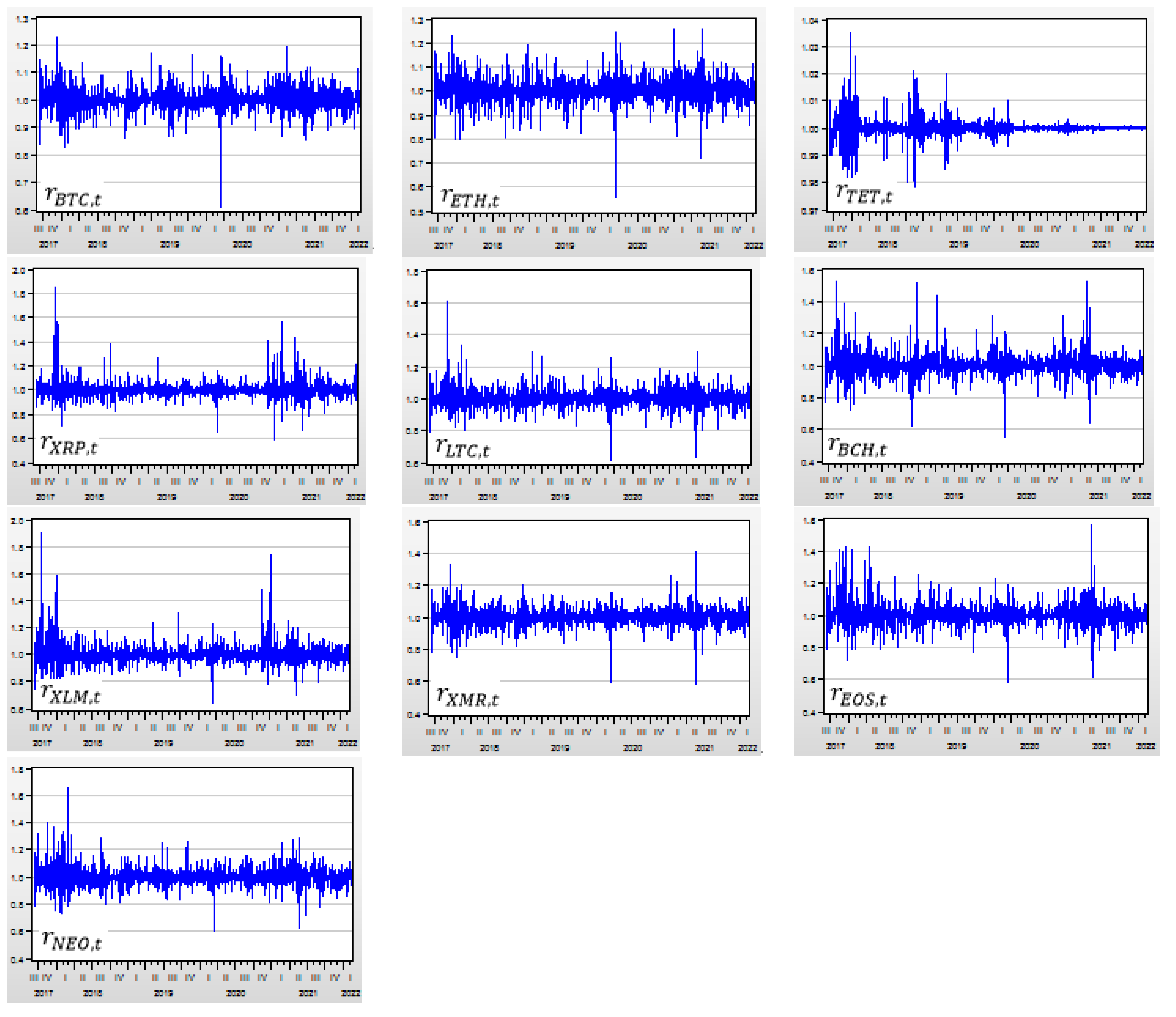
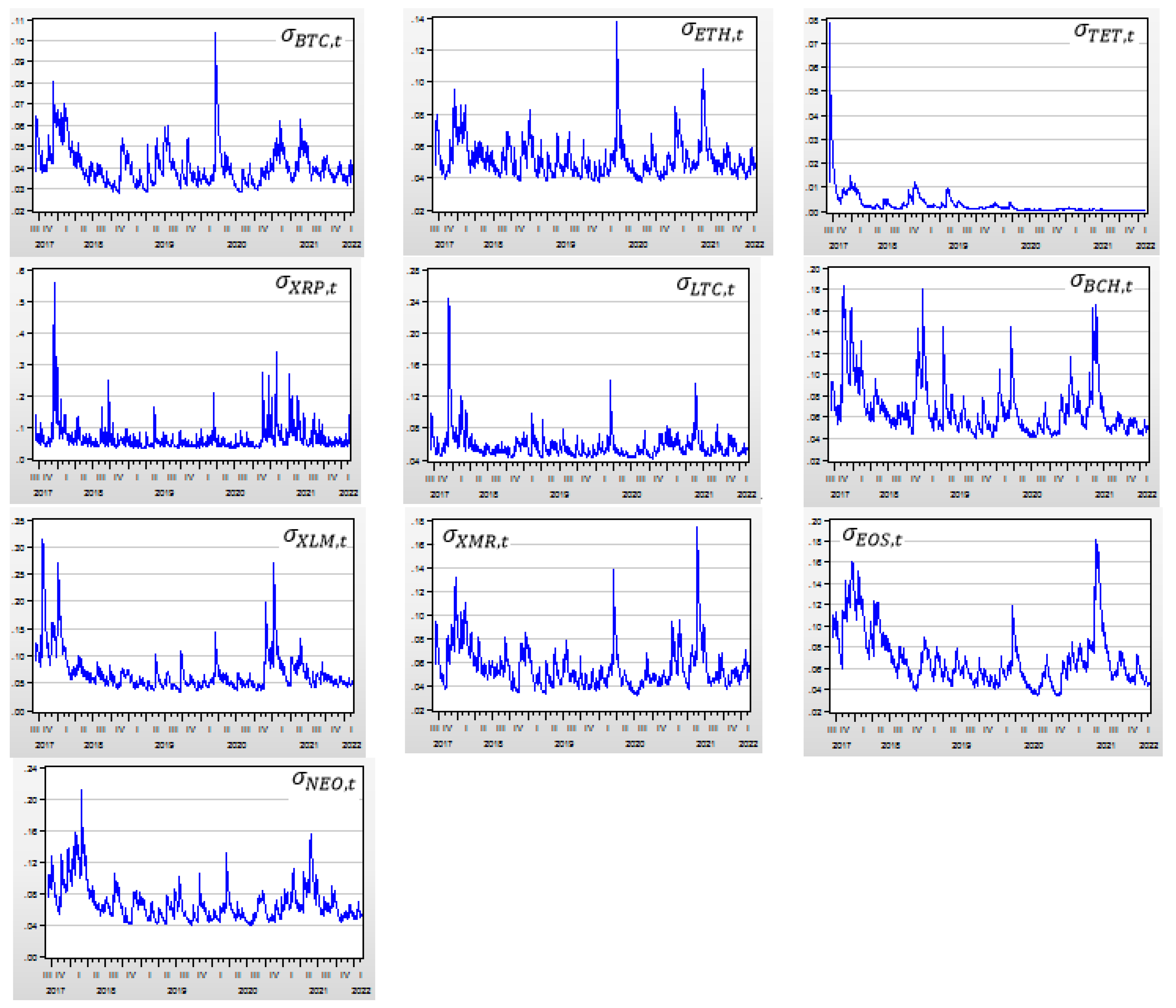
6.1. AR(1) and GARCH(1,1) Models

Table 8 lists the regression models of AR(1) and GARCH(1,1) for the 10 cryptocurrencies’ return indices during the full period.
It was proven that 7 out of 10 A R ( 1 ) models were statistically significant.
For each of the 10 models of A R ( 1 ) , the coefficient φ i , 1 represented the partial autocorrelation coefficient between r i , t and r i , t 1 .
For seven cryptocurrencies’ return indices, including Bitcoin, Ethereum, Tether, Ripple, Monero, EOS, and NEO, it was proven that the t-statistical values of the coefficient φ i , 1 had statistically substantial AR(1) models at the probability level of 1, 5, or 10%. Because the coefficient φ i , 1 of the AR(1) models of these seven cryptocurrencies was statistically substantial, the residuals of these models were directly applied to the GARCH(1,1) models.
For the other three cryptocurrencies’ return indices, including Litecoin, Bitcoin Cash, and Stellar, the t-statistical values of the coefficient φ i , 1 were not statistically substantial at the probability level of 1, 5, or 10%. Although the values of the three coefficients φ i , 1 of the AR(1) models were not statistically substantial, introducing the residual items into the GARCH(1,1) models would not matter if their coefficients were statistically substantial.
It was proven that all 10 GARCH(1,1) models were statistically significant.
It was important to guarantee that all of the GARCH(1,1) models were statistically substantial. For each GARCH ( 1 , 1 ) model of all 10 cryptocurrencies’ return indices, the t-statistic results proved that all three parameters of ω i , α i , and β i were statistically substantial at the probability level of 1%.
Because each AR(1) model had a residual item a i , t , when a i , t = σ i , t ε i , t , our focus aimed at analyzing the characteristics of the GARCH item σ i , t and the standard residual ε i , t .
The parameter β i was the coefficient of GARCH as the lag-1 item of σ i , t 1 . The coefficients of GARCH for Bitcoin, Ethereum, Tether, Ripple, Litecoin, Bitcoin Cash, Stellar, Monero, EOS, and NEO were 0.895008, 0.869725, 0.880962, 0.641374, 0.833616, 0.901260, 0.882065, 0.887105, 0.938592, and 0.899729, respectively. For all 10 GARCH(1,1) models, the values of coefficient β i were greater than 0.641374, which was quite high. This meant that the return indices of these 10 cryptocurrencies had features of volatility clustering or volatility spillover. Because all 10 GARCH(1,1) models were based on level variables, their volatilities had persistence or memory characteristics in the long run.
These results were similar to those of Soylu et al. (2020), Palamalai et al. (2020), Abakah et al. (2020), and Sensoy et al. (2020). Actually, the characteristics of clustering, spillover, and long memory in volatility were the same features. This meant that the fluctuations of the return index exhibited the tendency for larger fluctuations in returns to follow relatively larger fluctuations, while smaller fluctuations in returns will follow relatively smaller fluctuations (Palamalai et al. 2020).
Figure 2 depicts the curves of the GARCH values from the 10 cryptocurrencies’ return indices for the full period (8 September 2017–14 February 2022).
When the full time period was divided into the two periods of pre-COVID-19 and COVID-19, the characteristics of the GARCH values were differentiated.
Table 9 lists the results of the comparison of the average GARCH values of the 10 cryptocurrencies’ return indices for the three periods.
First, during the three time periods, Tether had the lowest GARCH values; inversely, the other nine cryptocurrencies had much higher GARCH values than Tether.
During the full period, the average GARCH value of Tether was 0.002857; however, the average GARCH values of the other nine cryptocurrencies were between 0.040666 and 0.069265.
During the pre-COVID-19 period, the average GARCH value of Tether was 0.004809; however, the average GARCH values of the other nine cryptocurrencies were between 0.041508 and 0.073962.
During the COVID-19 period, the average GARCH value of Tether was 0.000730; however, the average GARCH values of the other nine cryptocurrencies were between 0.039749 and 0.064930.
This meant that the volatility of Tether had less fluctuation than the other nine cryptocurrencies.
Second, when comparing the GARCH values between both periods of pre-COVID-19 and COVID-19, it was proven that the GARCH values of 8 out of 10 cryptocurrencies, including Bitcoin, Tether, Litecoin, Bitcoin Cash, Stellar, Monero, EOS, and NEO, decreased from the pre-COVID-19 period to the COVID-19 period.
From the pre-COVID-19 period to the COVID-19 period, the average GARCH values of Bitcoin, Tether, Litecoin, Bitcoin Cash, Stellar, Monero, EOS, and NEO decreased in differences of −0.001759, −0.004079, −0.001843, −0.009880, −0.008317, −0.002981, −0.010959, and −0.008727, respectively.
The differences in the GARCH values of Ethereum and Ripple between the pre-COVID-19 and COVID-19 periods were positive, but the differences were quite small at 0.000002 and 0.001926.
It was proven that COVID-19 caused the cryptocurrencies’ volatilities in the COVID-19 period to fluctuate less than in the pre-COVID-19 period. Since 2020, the volatilities of most of the cryptocurrencies have decreased. This means that most of the cryptocurrencies fluctuate less than before the beginning of COVID-19.
Third, from the correlations among the varying GARCH time series of the 10 cryptocurrencies, we found that the correlations were quite high. This result was similar to that of Le et al. (2021).
Table 10 lists the results of the correlations among the varying GARCH values of the 10 cryptocurrencies’ return indices for the full period.
For the full period, the average correlations between each of the 10 varying GARCH time series and the other 9 varying GARCH time series were 0.6470024, 0.6425153, 0.3233569, 0.4865397, 0.6103941, 0.6115659, 0.519619, 0.6720849, 0.6497457, and 0.6058991, respectively, for Bitcoin, Ethereum, Tether, Ripple, Litecoin, Bitcoin Cash, Stellar, Monero, EOS, and NEO. These correlations were quite high. These high correlations revealed that the volatilities of all 10 cryptocurrencies fluctuated in a similar fashion.
Fourth, the correlations among the varying GARCH time series of the 10 cryptocurrencies increased from the pre-COVID-19 period to the COVID-19 period.
Table 11 lists the results of the correlations among the varying GARCH values of the 10 cryptocurrencies’ return indices for the pre-COVID-19 period.
Table 12 lists the results of the correlations among the varying GARCH values of the 10 cryptocurrencies’ return indices for the COVID-19 period.
From the pre-COVID-19 period to the COVID-19 period, the average correlations between each of the 10 varying GARCH time series and the other 9 varying GARCH time series increased 0.0070144, 0.0859532, 0.00509, 0.1442054, 0.1644883, 0.0677548, 0.0246983, 0.0081004, and 0.112502, respectively, for Bitcoin, Ethereum, Tether, Litecoin, Bitcoin Cash, Stellar, Monero, EOS, and NEO, except for Ripple. These positive differences proved that from the pre-COVID-19 period to the COVID-19 period, the correlations among the varying GARCH value time series increased.
This meant that COVD-19 increased the correlations among the different cryptocurrencies’ dynamic volatilities. It was proven that the trends of cryptocurrencies’ dynamic volatilities moved in a similar pattern.
Fifth, for the pre-COVID-19 period, the highest GARCH values occurred during 2017–2018. For the COVID-19 period, the highest GARCH values occurred during March 2020. Although the highest GARCH values were not avoidable during the COVID-19 period, the average GARCH values decreased, and the correlations among the varying GARCH time series of the 10 cryptocurrencies increased.

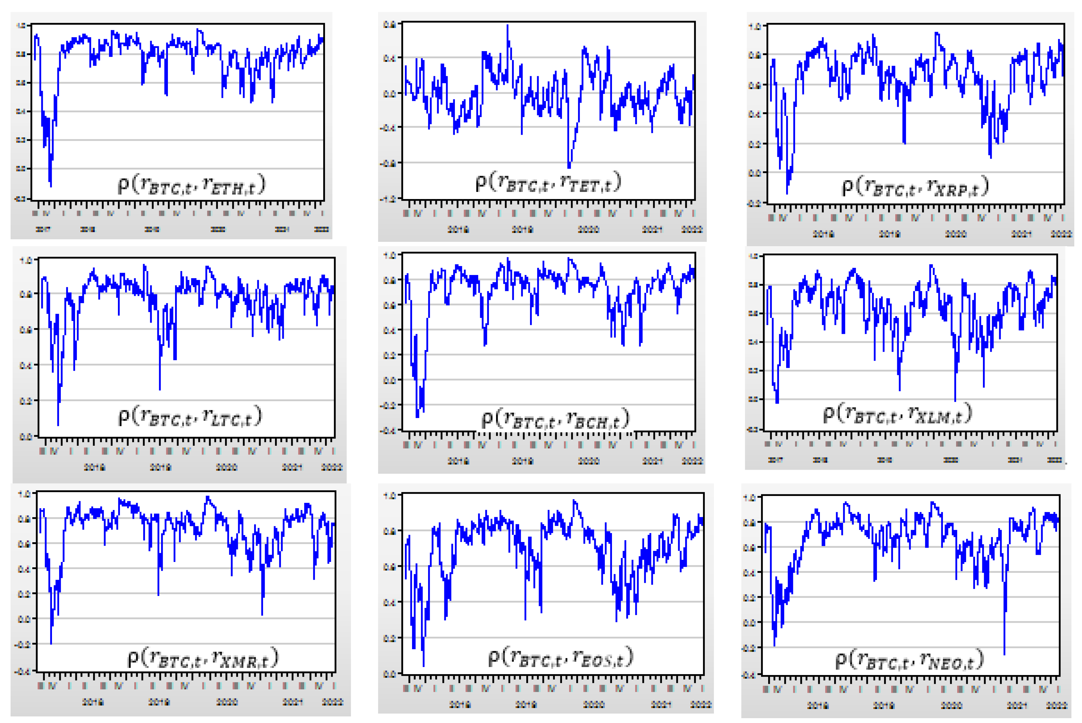
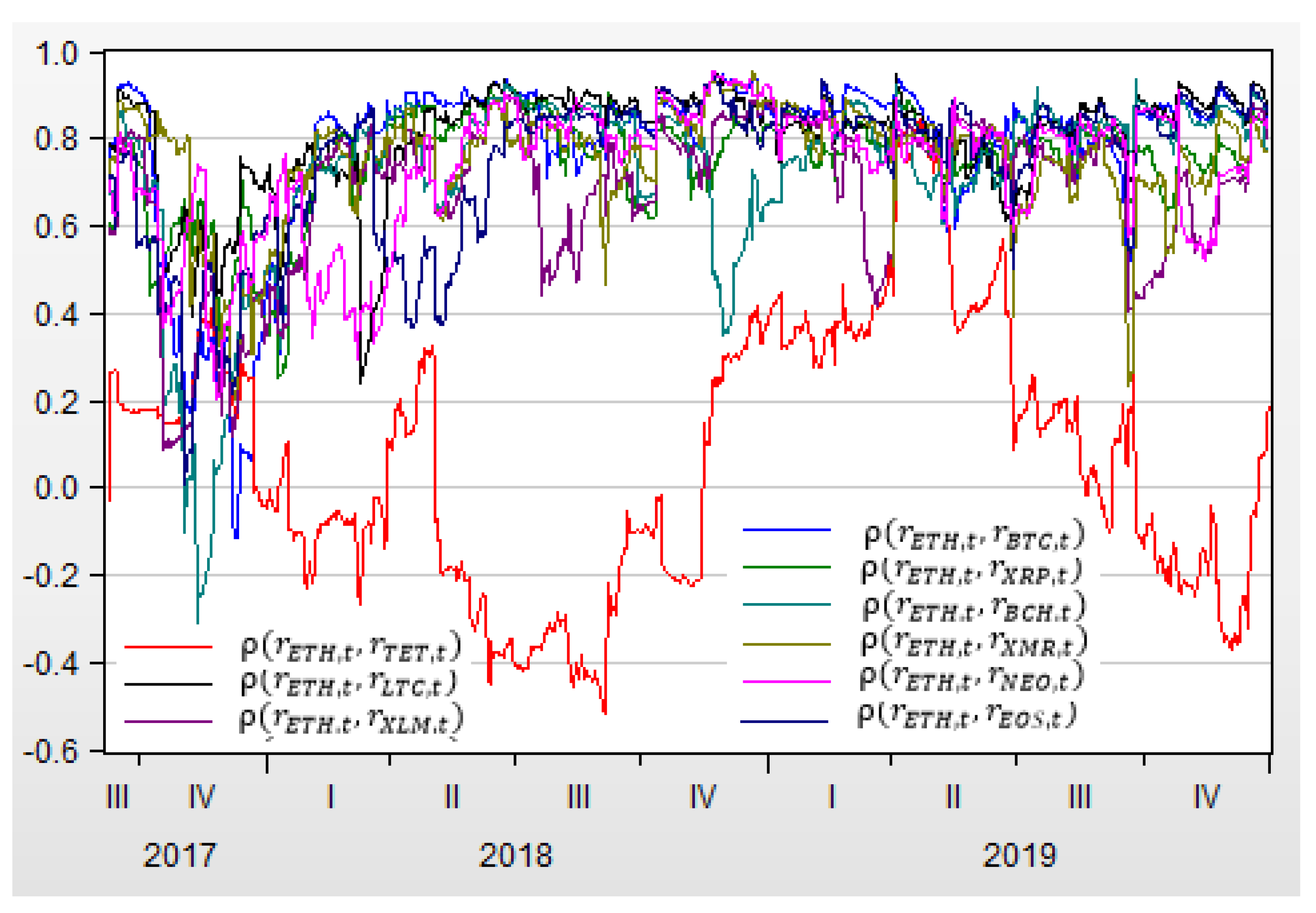
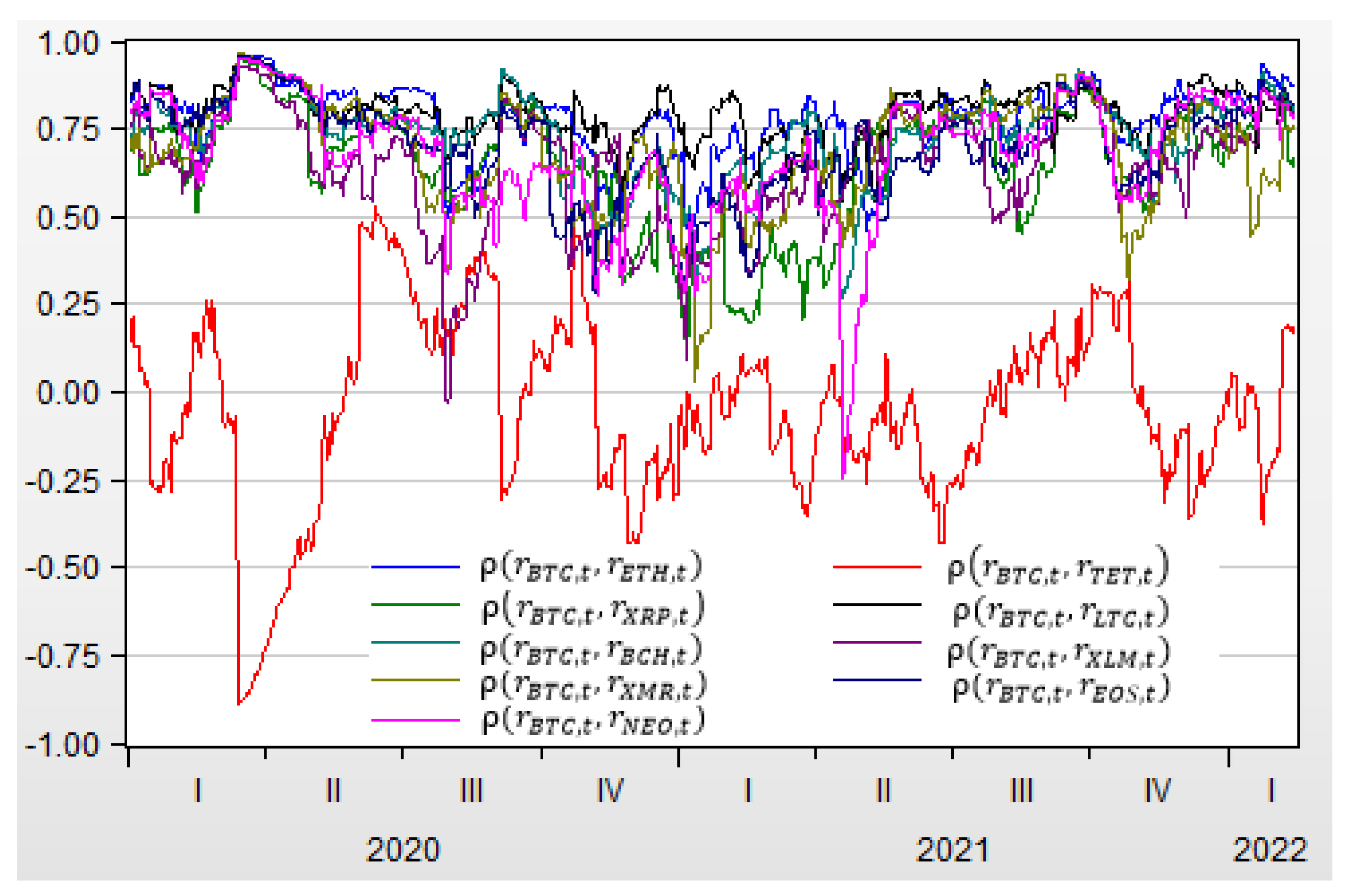
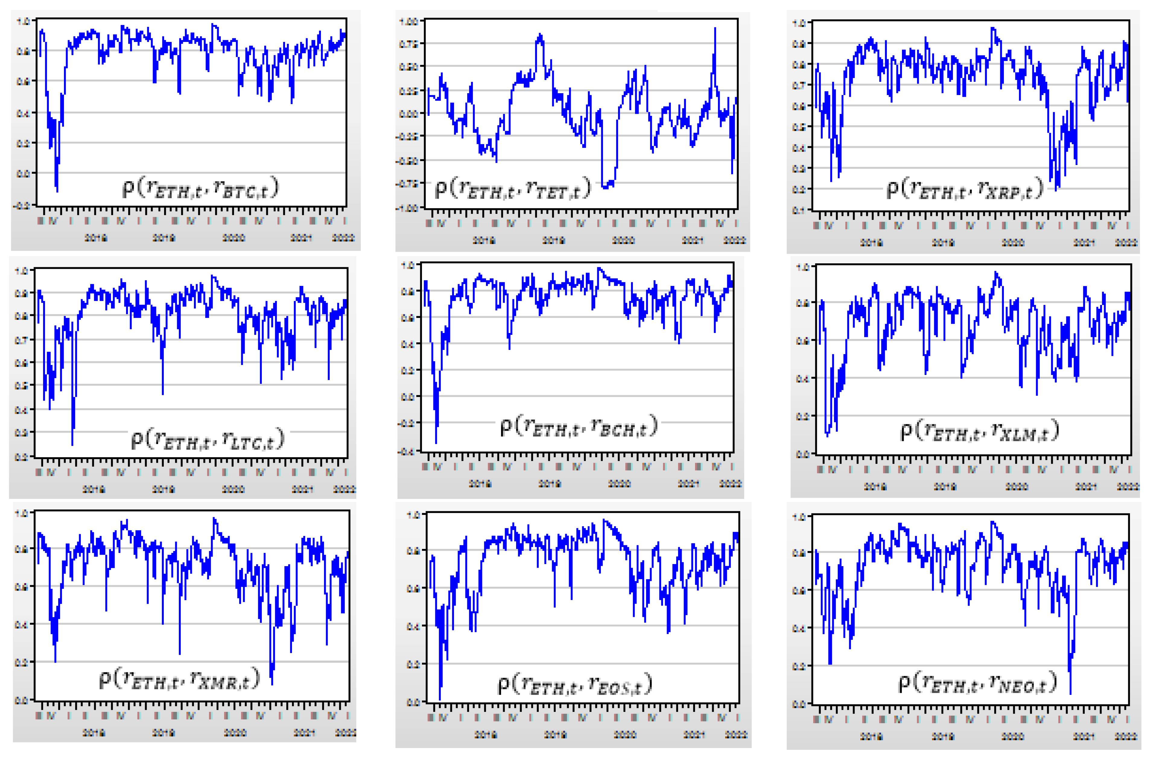
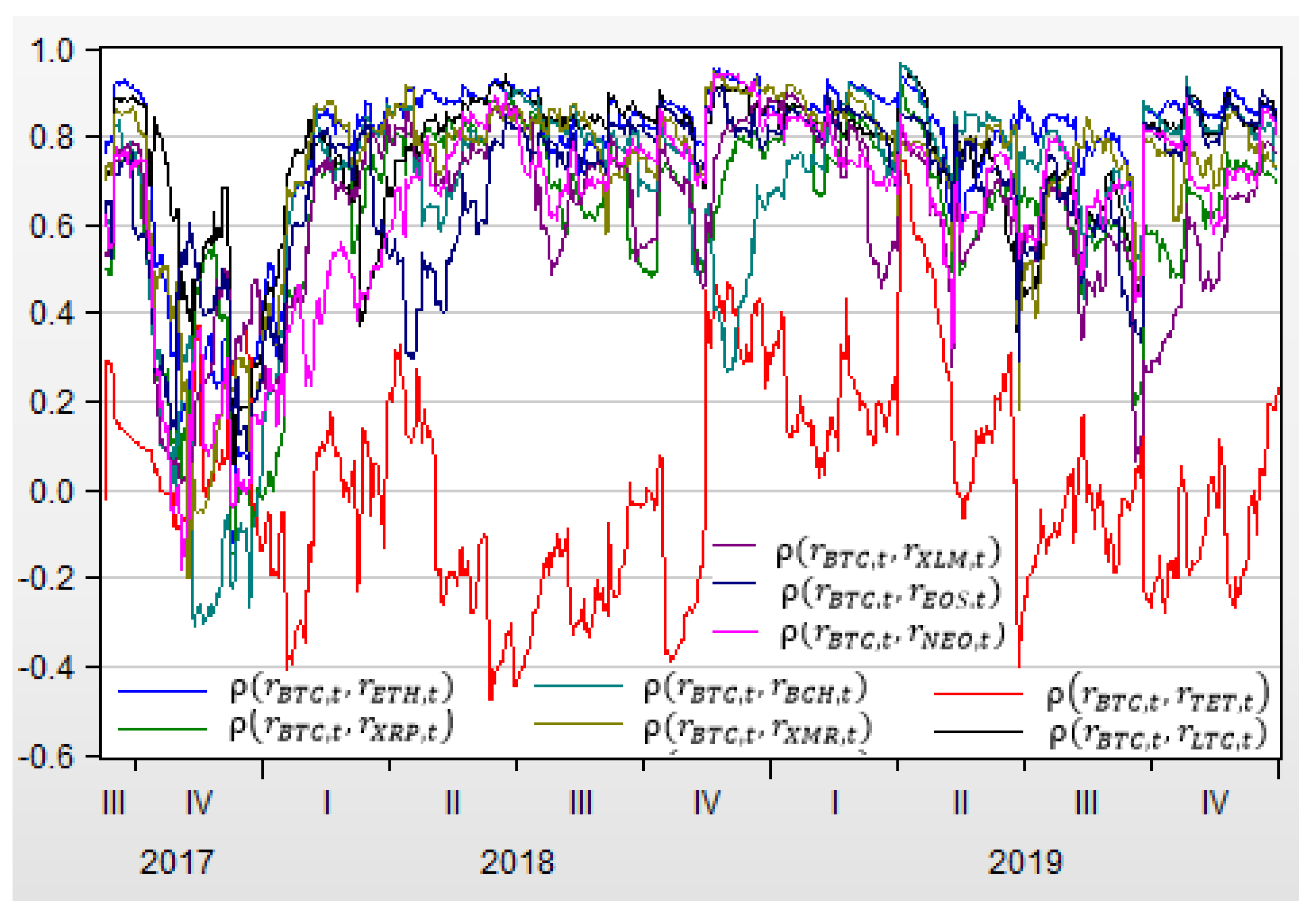
6.2. DCC(1,1) Models

Generally, a dynamic conditional correlation (DCC) was calculated from two varying time series variables. Because Bitcoin and Ethereum were the two most representative cryptocurrencies, we built the empirical models of the DCC(1,1) between the return indices of Bitcoin and Ethereum and the other cryptocurrencies.
Table 13 lists the results of the DCC(1,1) models built between the return indices of Bitcoin and Ethereum and the other cryptocurrencies’ return indices for the full period.
For all of the DCC(1,1) models, the t-statistic values proved that all of their coefficients represented by α and β were statistically substantial at the probability level of 1%. Substantially, these 18 DCC(1,1) models were used to analyze the characteristics of the dynamic varying correlations.
Figure 3 depicts the curves of the DCC between Bitcoin and the other nine cryptocurrencies for the full period.
Figure 4 depicts the curves of the DCC between Ethereum and the other eight cryptocurrencies for the full period.
Table 14 lists the comparison results of the mean values of DCC(1,1) between the return indices of Bitcoin and Ethereum and the other cryptocurrencies for the three periods.
First, except for Tether, during the full time period the varying correlations between the return indices of Bitcoin and Ethereum and the other eight cryptocurrencies from the descriptive statistics were positive and quite high.
For the full period, except for Tether, the mean values of the DCC between Bitcoin and the other eight cryptocurrencies were between 0.6243 and 0.7783; the mean values of the DCC between Ethereum and the other cryptocurrencies were between 0.7393 and 0.8038.
This result was similar to the research of Ciaian et al. (2018) and Lahajnar and Rozanec (2020) and proved that the correlations between Bitcoin and the other cryptocurrencies were strong.
Second, the correlations between Ethereum and the other cryptocurrencies were higher than the correlations between Bitcoin and the other cryptocurrencies.
Figure 4 depicts the curves of the DCC between Ethereum and the other eight cryptocurrencies for the full period.
Figure 3 depicts the curves of the DCC between Bitcoin and the other nine cryptocurrencies for the full period.
During the full period, except for Tether, the average varying correlations between the return indices of Bitcoin and the other cryptocurrencies, including Ripple, Litecoin, Bitcoin Cash, Stellar, Monero, EOS, and NEO, were 0.63941, 0.773738, 0.699301, 0.624351, 0.708394, 0.690766, and 0.658295, respectively; otherwise, the average varying correlations between the return indices of Ethereum and the other cryptocurrencies, including Ripple, Litecoin, Bitcoin Cash, Stellar, Monero, EOS, and NEO, were 0.725803, 0.803866, 0.740293, 0.681546, 0.714453, 0.740066, and 0.730576, respectively; in comparison, the differences between both groups of correlations were 0.086393, 0.030128, 0.040992, 0.057195, 0.006059, 0.049300, and 0.072281. It was clear that the average values of the DCC between Ethereum and the other cryptocurrencies were higher than the average values of the DCC between Bitcoin and the other cryptocurrencies.
This means that Ethereum has become a more important representative cryptocurrency than Bitcoin or that Ethereum has a higher impact on the other cryptocurrencies than Bitcoin.
Third, except for Tether, when comparing the changes in the DCC mean values between the pre-COVID-19 period and the COVID-19 period, since the COVID-19 pandemic began, the average DCC values between Bitcoin and the other cryptocurrencies have increased.
Figure 5 depicts the curves of the DCC between Bitcoin and the other nine cryptocurrencies for the pre-COVID-19 period.
Figure 6 depicts the curves of the DCC between Ethereum and the other eight cryptocurrencies for the pre-COVID-19 period.
Figure 7 depicts the curves of the DCC between Bitcoin and the other nine cryptocurrencies for the COVID-19 period.
Figure 8 depicts the curves of the DCC between Ethereum and the other eight cryptocurrencies for the COVID-19 period.
During the pre-COVID-19 period, except for Tether, the average varying correlations between the return indices of Bitcoin and the other cryptocurrencies, including Ripple, Litecoin, Bitcoin Cash, Stellar, EOS, and NEO, were 0.633941, 0.754496, 0.672014, 0.615718, 0.685013, and 0.642678, respectively.
During the COVID-19 period, except for Tether, the average varying correlations between the return indices of Bitcoin and the other cryptocurrencies, including Ripple, Litecoin, Bitcoin Cash, Stellar, EOS, and NEO, were 0.645365, 0.794691, 0.729014, 0.633752, 0.697030, and 0.675301, respectively.
From the pre-COVID-19 period to the COVID-19 period, except for Tether, the average varying correlations between the return indices of Bitcoin and the other cryptocurrencies, including Ripple, Litecoin, Bitcoin Cash, Stellar, EOS, and NEO, increased by differences of 0.011424, 0.040195, 0.057000, 0.018034, 0.012017, and 0.032623, respectively.
This means that the correlations between Bitcoin and the other cryptocurrencies have enhanced since the beginning of 2020.
However, these correlations were not proven for Ethereum.
Fourth, except for Tether, from the correlations among the varying DCC values between Bitcoin and Ethereum, and between Bitcoin, Ethereum, and the other cryptocurrencies, we determined that the correlations among these cryptocurrencies were similar to those of Bitcoin and Ethereum.
The correlations among the varying DCC value time series between Bitcoin and Ethereum and the varying DCC value time series between Bitcoin and Ripple, Litecoin, Bitcoin Cash, Stellar, Monero, EOS, and NEO were 0.761078, 0.727885, 0.808231, 0.680740, 0.787096, 0.715787, and 0.839999, respectively, which were quite high.
The correlations among the varying DCC value time series between Ethereum and Bitcoin and the varying DCC value time series between Ethereum and Ripple, Litecoin, Bitcoin Cash, Stellar, Monero, EOS, and NEO were 0.587975, 0.620270, 0.739476, 0.732984, 0.627493, 0.666690, and 0.541859, respectively, which were also quite high.
It was clear that the trend changes in the DCC value time series between Bitcoin, Ethereum, and the other cryptocurrencies were similar.
Fifth, we determined the differences of the other cryptocurrencies from Tether, whose characteristics were quite different.
For the full period, the average DCC values between the return indices of Bitcoin and Tether were negative, being −0.01701 for the full period, 0.0131 for the pre-COVID-19 period, and −0.0500 for the COVID-19 period. For the full period, the correlations among the DCC value time series between Bitcoin and Tether and the DCC value time series between Bitcoin and the other cryptocurrencies, including Ethereum, Ripple, Litecoin, Bitcoin Cash, Stellar, Monero, EOS, and NEO, were negative at −0.081714, −0.029559, −0.099312, −0.145631, −0.067753, −0.054917, −0.094690, and −0.069847, respectively.
For the full period, the correlations between the return index of Tether and the other cryptocurrencies, including Bitcoin, Ethereum, Ripple, Bitcoin Cash, Stellar, Monero, and EOS, were negative at −0.021680, −0.026539, −0.032471, −0.034959, −0.034237, −0.022461, and −0.022924.
For the pre-COVID-19 period, the correlations between the return index of Tether and the other cryptocurrencies, including Bitcoin, Ethereum, Ripple, Bitcoin Cash, Stellar, Monero, and EOS, were 0.010457, 0.001710, −0.018437, −0.014268, −0.022881, 0.005238, and −0.003722, respectively. Although the static correlations between the return indices of Tether and the other cryptocurrencies were not always negative, the maximum values of the static correlations were less than 0.010457.
For the COVID-19 period, the correlations between the return index of Tether and the other cryptocurrencies, including Bitcoin, Ethereum, Ripple, Bitcoin Cash, Stellar, Monero, and EOS, were negative at −0.243461, −0.221253, −0.155334, −0.214276, −0.148999, −0.219096, and −0.175636, respectively. This means that the correlations between the return index of Tether and most of the other cryptocurrencies were negative.
From the pre-COVID-19 period to the COVID-19 period, on average, the correlations between Tether and the other cryptocurrencies changed from negative or very small to negative; Tether became a highly hedging cryptocurrency against the other cryptocurrencies.
Because the correlations between the return indices of Tether and the other cryptocurrencies were mostly negative or very low, Tether can be a hedge cryptocurrency against the other cryptocurrencies. This result was totally different from the research of Kyriazis et al. (2019) because they confirmed that no hedging abilities existed among cryptocurrencies. COVID-19 has enhanced the degree of negative correlations, or it has increased the hedging characteristics between Tether and the other cryptocurrencies.

7. Summary and Further Studies

This paper focused on studying the relationship between Bitcoin, Ethereum, and the other eight cryptocurrencies, including Tether, Ripple, Litecoin, Bitcoin Cash, Stellar, Monero, EOS, and NEO. The observation sample data covered the full time period from 8 September 2017 to 14 February 2022, with 1621 observations, and covered the time when the full period was divided into the pre-COVID-19 period from 8 September 2017 to 31 December 2019, with 845 observations, and the COVID-19 period from 1 January 2020 to 14 February 2022, with 776 observations.
After an empirical analysis, we arrived at four main results.
First, the descriptive statistics and tests proved that, from the pre-COVID-19 period to the COVID-19 period, almost all of the 10 cryptocurrencies’ growth rates increased; thus, COVID-19 had a positive effect on the returns of cryptocurrencies.
Second, from the empirical results of the GARCH(1,1) models, we proved that, for all of the 10 GARCH(1,1) models, the values of the coefficient β i were greater than 0.641374, which means that these 10 cryptocurrencies’ return indices had features of volatility clustering or memory persistence in the long run. This result was similar to those of Soylu et al. (2020), Palamalai et al. (2020), Abakah et al. (2020), and Sensoy et al. (2020). Tether had the lowest GARCH values, but the other nine cryptocurrencies had higher GARCH values than Tether; all of the 10 cryptocurrencies’ GARCH values decreased from the pre-COVID-19 period to the COVID-19 period. The correlations among the varying GARCH time series of the 10 cryptocurrencies were quite high and were similar to the findings of Le et al. (2021). The correlations among the varying GARCH time series of the 10 cryptocurrencies increased from the pre-COVID-19 period to the COVID-19 period. The trends of cryptocurrencies’ dynamic volatilities moved in a similar pattern: for the pre-COVID-19 period, the highest GARCH values occurred during 2017–2018; for the COVID-19 period, the highest GARCH values occurred during March 2020.
Third, from the empirical results of the DCC(1,1) models, we proved that, except for Tether, the varying correlations between the return indices of Bitcoin, Ethereum, and the other cryptocurrencies were very strong, similar to the findings of Ciaian et al. (2018) and Lahajnar and Rozanec (2020). They proved that the correlations between Bitcoin and the other cryptocurrencies were strong; the correlations between Ethereum and the others were higher than between Bitcoin and the others. Since the COVID-19 pandemic began, the average values of the DCC between Bitcoin and the other cryptocurrencies, except Tether, have increased; except for Tether, since the COVID-19 pandemic began, the correlations among the 10 cryptocurrencies’ return indices have become higher than before.
Fourth, the characteristics of Tether were quite different from those of the other cryptocurrencies: during the COVID-19 period, the static correlations between the return indices of Tether and the other nine cryptocurrencies were negative; during the pre-COVID-19 period and the full period, the static correlations between the return indices of Tether and the other cryptocurrencies were not always negative but were very low at less than 0.010457. Tether can act as a hedge cryptocurrency for the other cryptocurrencies, and this result differed from the research of Kyriazis et al. (2019) because they found that no hedging abilities existed among cryptocurrencies.

Author Contributions

Conceptualization, K.Y. and H.Y.; methodology, K.Y. and H.Y.; software, K.Y. and H.Y.; validation, K.Y. and H.Y.; formal analysis, K.Y. and H.Y.; investigation, K.Y. and H.Y.; resources, K.Y. and H.Y.; data curation, K.Y. and H.Y.; writing—original draft preparation, K.Y. and H.Y.; writing—review and editing, H.Y. and H.Y.; visualization, K.Y. and H.Y.; supervision, H.Y. and R.G.; project administration, K.Y. All authors have read and agreed to the published version of the manuscript.

Funding

This research received no external funding.

Institutional Review Board Statement

Not applicable.

Informed Consent Statement

Not applicable.

Data Availability Statement

The open data source cn.investing.com (accessed on 17 February 2022) is used as data sources for this paper.

Conflicts of Interest

The authors declare no conflict of interest.

References

  1. Abakah, Emmanuel Joel Aikins, Luis Alberiko Gil-Alana, Godfrey Madigu, and Fatima Romero-Rojo. 2020. Volatility persistence in cryptocurrency markets under structural breaks. International Review of Economics and Finance 69: 680–91. [Google Scholar] [CrossRef]
  2. Ardia, David, Keven Bluteau, and Maxime Rüede. 2019. Regime changes in Bitcoin GARCH volatility dynamics. Finance Research Letters 29: 266–71. [Google Scholar]
  3. Będowska-Sójka, Barbara, Tomasz Hinc, and Agata Kliber. 2019. Causality between Volatility and Liquidity in Cryptocurrency Market. Working Paper. [Google Scholar] [CrossRef]
  4. Box, George E. P., and David A. Pierce. 1970. Distribution of residual correlations in autoregressive-integrated moving average time series models. Journal of the American Statistical Association 65: 1509–26. [Google Scholar] [CrossRef]
  5. Caporale, Guglielmo Maria, and Timur Zekokh. 2019. Modelling volatility of cryptocurrencies using Markov Switching GARCH models. Research in International Business and Finance 48: 143–55. [Google Scholar] [CrossRef]
  6. Ciaian, Pavel, Miroslava Rajcaniova, and Artis Kancs. 2018. Virtual relationships: Short- and long-run evidence from BitCoin and altcoin markets. Journal of International Financial Markets, Institutions & Money 52: 173–95. [Google Scholar]
  7. Corbet, Shaen, Yang Hou, Yang Hu, Charles Larkin, and Larkin Oxley. 2020. Any port in a storm: Cryptocurrency safe-havens during the COVID-19 pandemic. Economics Letters 194: 109377. [Google Scholar] [CrossRef]
  8. Dickey, David A., and Wayne A. Fuller. 1979. Distribution of the estimators for time series with a unit root. Journal of the American Statistical Association 74: 427–31. [Google Scholar]
  9. Dickey, David A., and Wayne A. Fuller. 1981. Likelihood ratio statistics for autoregressive time series with a unit root. Econometrica 49: 1057–72. [Google Scholar] [CrossRef]
  10. Dilek, Teker, Teker Suat, and Ozyesil Mustafa. 2020. Macroeconomic determinants of cryptocurrency volatility: Time series analysis. Journal of Business & Economic Policy 7: 65–77. [Google Scholar] [CrossRef]
  11. Engle, Robert F. 1982. Autoregressive conditional heteroscedasticity with estimates of the variance of United Kingdom inflations. Econometria 50: 987–1007. [Google Scholar] [CrossRef]
  12. Engle, Robert. 2002. Dynamic Conditional Correlation—A Simple Class of Multivariate GARCH models. Journal of Business and Economic Statistics 20: 339–50. [Google Scholar] [CrossRef]
  13. Enoksen, F. A., C. J. Landsnes, K. Lucivjanská, and P. Molnár. 2020. Understanding risk of bubbles in cryptocurrencies. Journal of Economic Behavior and Organization 176: 129–44. [Google Scholar] [CrossRef]
  14. García-Medina, Andrés, and José B. Hernández C. 2020. Network analysis of multivariate transfer entropy of cryptocurrencies in times of turbulence. Entropy 22: 760. [Google Scholar] [CrossRef] [PubMed]
  15. Huynh, Toan Luu Duc, Muhammad Ali Nasir, Xuan Vinh Vo, and Thong Trung Nguyen. 2020. Small things matter most: The spillover effects in the cryptocurrency market and gold as a silver bullet. North American Journal of Economics and Finance 54: 101277. [Google Scholar] [CrossRef]
  16. İçellioğlu, Cansu Şarkaya, and Selma Öner. 2019. An investigation on the volatility of cryptocurrencies by means of heterogeneous panel data Analysis. Procedia Computer Science 158: 913–20. [Google Scholar] [CrossRef]
  17. IFRSIC. 2019. Committee’s Tentative Agenda Decisions on Holdings of Cryptocurrencies. IFRS Interpretations Committee (IC), Update March 2019. Available online: https://www.ifrs.org/news-and-events/updates/IFRSIC-updates/march-2019/#1 (accessed on 9 September 2020).
  18. Investing. 2022. Today’s Cryptocurrency Prices. Available online: https://cn.investing.com/crypto/currencies (accessed on 18 February 2022).
  19. Iqbal, Najaf, Zeeshan Fareed, Guangcai Wan, and Farruskh Shahzad. 2021. Asymmetric nexus between COVID-19 outbreak in the world and cryptocurrency market. International Review of Financial Analysis 73: 101613. [Google Scholar] [CrossRef]
  20. James, Nick, Max Menzies, and Jennifer Chan. 2021. Changes to the extreme and erratic behaviour of cryptocurrencies during COVID-19. Physica A 565: 125581. [Google Scholar] [CrossRef]
  21. Kyriazis, Nikolaos A., Kalliopi Daskalou, Marios Arampatzis, Paraslevi Prassa, and Evangelia Papaioannou. 2019. Estimating the volatility of cryptocurrencies during bearish markets byemploying GARCH models. Heliyon 5: e02239. [Google Scholar] [CrossRef]
  22. Lahajnar, Sebastian, and Alenka Rozanec. 2020. The correlation strength of the most important cryptocurrencies in the bull and bear market. Investment Management and Financial Innovations 17: 67–81. [Google Scholar] [CrossRef]
  23. Le, TN-Lan, Emmanuel Joel Aikins Abakah, and Aviral Kumar Tiwari. 2021. Time and frequency domain connectedness and spill-over among fintech, green bonds and cryptocurrencies in the age of the fourth industrial revolution. Technological Forecasting & Social Change 162: 120382. [Google Scholar]
  24. Ljung, Greta Marianne, and George Edward Pelham Box. 1978. On a measure of lack of fit in time series models. Biometrika 66: 67–72. [Google Scholar] [CrossRef]
  25. Palamalai, Srinivasan, K. Krishna Kumar, and Bipasha Maity. 2020. Testing the random walk hypothesis for leading cryptocurrencies. Borsa Istanbul Review 21: 256–68. [Google Scholar] [CrossRef]
  26. Sensoy, Ahmet, Thiago Christiano Silva, Shaen Corbet, and Benjamin Miranda Tabak. 2020. High-Frequency Return and Volatility Spillovers among Cryptocurrencies. Researchgate, June. Available online: https://www.researchgate.net/publication/341820733 (accessed on 30 November 2020).
  27. Siswantoro, Dpdik, Rangga Handika, and Aria Farah Mita. 2020. The requirements of cryptocurrency for money, an Islamic view. Heliyon 6: e03235. [Google Scholar] [CrossRef] [Green Version]
  28. Soylu, Pinar Kaya, Mustafa Okur, Ozgur Çatıkkaş, and Ayca Altintig. 2020. Long memory in the volatility of selected cryptocurrencies: Bitcoin, Ethereum and Ripple. Journal of Risk and Financial Management 13: 107. [Google Scholar] [CrossRef]
  29. Wooldridge, Jeffrey M. 2000. Introductory Econometrics: A Modern Approach. Chula Vista: South Western College, ISBN 0-538-85013-2. [Google Scholar]
Figure 1. Curves of the return index for each of the 10 cryptocurrencies for the full period (8 September 2017–14 February 2022).
Jrfm 15 00113 g001
Figure 2. Curves of GARCH values from the 10 cryptocurrencies’ return indices for the full period (8 September 2017–14 February 2022).
Jrfm 15 00113 g002
Figure 3. Curves of DCC between Bitcoin and the other nine cryptocurrencies for the full period.
Jrfm 15 00113 g003
Figure 4. Curves of the DCC between Ethereum and the other eight cryptocurrencies for the full period.
Jrfm 15 00113 g004
Figure 5. Curves of the DCC between Bitcoin and the other nine cryptocurrencies for the pre-COVID-19 period.
Jrfm 15 00113 g005
Figure 6. Curves of the DCC between Ethereum and the other eight cryptocurrencies for the pre-COVID-19 period.
Jrfm 15 00113 g006
Figure 7. Curves of the DCC between Bitcoin and the other nine cryptocurrencies for the COVID-19 period.
Jrfm 15 00113 g007
Figure 8. Curves of the DCC between Ethereum and the other eight cryptocurrencies for the COVID-19 period.
Jrfm 15 00113 g008
Table 1. Ranking, price, market cap, and 24 h trading volume of the 10 cryptocurrencies in the global market on 18 February 2022.
RankingCryptocurrencyAbbreviationPrice (USD)Market Capitalization24 h Trading Volume
Market Cap (USD)Ratio (%)24 h Volume (USD)Ratio (%)
1Bitcoin B T C 40782771.32B41.69%17.460000B30.68%
2Ethereum E T H 2899.3347.288B18.77%13.210000B23.21%
3Tether (USDT) T E T 1.00978.73B4.26%2.616600B4.60%
6Ripple X R P 0.7879337.74B2.04%0.139910B0.25%
20Litecoin L T C 1178.15B0.44%0.115070B0.20%
28Bitcoin Cash B C H 313.85.96B0.32%0.077834B0.14%
31Stellar X L M 0.204985.11B0.28%0.034826B0.06%
45Monero X M R 164.382.98B0.16%0.028847B0.05%
48EOS E O S 2.35592.31B0.12%0.051469B0.09%
58NEO N E O 24.591.73B0.09%0.020801B0.04%
Sum of the 10 cryptocurrencies1261.318B68.18%33.755357B59.32%
Total 10,707 cryptocurrencies1850B100.00%56.906B100.00%
Note: B represents USD 1 billion.
Table 2. Descriptive statistics of the 10 cryptocurrencies’ return indices for the full period.
Stats r B T C , t r E T H , t r T E T , t r X R P , t r L T C , t r B C H , t r X L M , t r X M R , t r E O S , t r N E O , t
Mean1.0023 1.0028 1.0000 1.0031 1.0021 1.0020 1.0041 1.0018 1.0031 1.0023
Growth0.2295%0.2813%−0.0006%0.3111%0.2097%0.2007%0.4058%0.1835%0.3116%0.2299%
Median1.0015 1.0015 1.0000 1.0001 0.9995 0.9988 1.0000 1.0026 1.0000 1.0010
Maximum1.2255 1.2596 1.0352 1.8558 1.6106 1.5291 1.8977 1.4080 1.5618 1.6605
Minimum0.6082 0.5545 0.9787 0.5822 0.6146 0.5501 0.6438 0.5854 0.5801 0.5996
Std. Dev.0.0418 0.0527 0.0034 0.0705 0.0601 0.0699 0.0745 0.0558 0.0713 0.0701
Skewness−0.2508 −0.2809 0.7773 2.6610 1.0338 1.1259 2.6139 −0.1714 1.0374 0.8436
Kurtosis10.23 8.77 22.64 28.64 15.55 14.29 27.45 10.46 11.95 11.87
Jarque–Bera3544 2268 26,225 46,333 10,935 8947 42,217 3767 5696 5501
Probability0.0000 0.0000 0.0000 0.0000 0.0000 0.0000 0.0000 0.0000 0.0000 0.0000
Obs1621162116211621162116211621162116211621
Table 3. Descriptive statistics of the 10 cryptocurrencies’ return indices for the pre-COVID-19 period.
Stats r B T C , t r E T H , t r T E T , t r X R P , t r L T C , t r B C H , t r X L M , t r X M R , t r E O S , t r N E O , t
Mean1.0015 1.0003 1.0000 1.0021 1.0012 1.0015 1.0040 1.0005 1.0041 1.0015
Growth0.1523%0.0338%−0.0007%0.2064%0.1154%0.1482%0.3983%0.0465%0.4067%0.1468%
Median1.0007 0.9989 1.0000 0.9987 0.9964 0.9962 0.9972 0.9993 0.9985 0.9974
Maximum1.2255 1.2322 1.0352 1.8558 1.6106 1.5291 1.8977 1.3268 1.4275 1.6605
Minimum0.8295 0.7982 0.9787 0.7019 0.7350 0.6193 0.7226 0.7471 0.7202 0.7347
Std. Dev.0.0430 0.0519 0.0046 0.0704 0.0626 0.0760 0.0805 0.0566 0.0759 0.0762
Skewness0.2694 0.0319 0.5858 3.9068 2.1114 1.3783 2.8195 0.1439 1.3027 1.4692
Kurtosis6.0744 5.5172 12.6270 40.0922 19.2643 12.3852 26.7278 6.1820 9.4422 12.7413
Jarque–Bera343.01 223.23 3311.42 50,590.19 9941.45 3368.73 20,942.07 359.40 1700.21 3645.00
Probability0.0000 0.0000 0.0000 0.0000 0.0000 0.0000 0.0000 0.0000 0.0000 0.0000
Observations845845845845845845845845845845
Table 4. Descriptive statistics of the 10 cryptocurrencies’ return indices for the COVID-19 period.
Stats r B T C , t r E T H , t r T E T , t r X R P , t r L T C , t r B C H , t r X L M , t r X M R , t r E O S , t r N E O , t
Mean1.0031 1.0055 1.0000 1.0043 1.0031 1.0026 1.0041 1.0033 1.0021 1.0032
Growth0.3134%0.5493%−0.0015%0.4251%0.3114%0.2580%0.4130%0.3292%0.2071%0.3179%
Median1.0024 1.0043 1.0000 1.0020 1.0027 1.0021 1.0026 1.0054 1.0012 1.0034
Maximum1.1941 1.2596 1.0102 1.5667 1.2923 1.5283 1.7395 1.4080 1.5618 1.2893
Minimum0.6082 0.5545 0.9933 0.5822 0.6146 0.5501 0.6438 0.5854 0.5801 0.5996
Std. Dev.0.0403 0.0534 0.0009 0.0707 0.0572 0.0627 0.0674 0.0549 0.0660 0.0629
Skewness−0.9294 −0.6023 0.3948 1.3228 −0.5074 0.6062 2.1484 −0.5412 0.5645 −0.3788
Kurtosis16.0985 12.0773 37.5916 16.5720 9.6452 17.1891 26.4363 15.8050 15.9871 8.6374
Jarque–Bera5659.13 2711.08 38,709.61 6182.08 1461.10 6557.19 18,3565339.53 5494.72 1046.1
Probability0.0000 0.0000 0.0000 0.0000 0.0000 0.0000 0.0000 0.0000 0.0000 0.0000
Observations776776776776776776776776776776
Table 5. Comparison of the average growth rates of the 10 cryptocurrencies’ return indices in percentages for the three periods.
Return IndexPre_COVID-19 (1)COVID-19 (2)Full Period (3)(2)–(1)(2)–(3)
r B T C , t 0.1523%0.3134%0.2295%0.1611%0.0839%
r E T H , t 0.0338%0.5493%0.2813%0.5155%0.2680%
r T E T , t −0.0007%−0.0015%−0.0006%−0.0008%−0.0009%
r X R P , t 0.2064%0.4251%0.3111%0.2187%0.1140%
r L T C , t 0.1154%0.3114%0.2097%0.1960%0.1017%
r B C H , t 0.1482%0.2580%0.2007%0.1098%0.0573%
r X L M , t 0.3983%0.4130%0.4058%0.0147%0.0072%
r X M R , t 0.0465%0.3292%0.1835%0.2827%0.1457%
r E O S , t 0.4067%0.2071%0.3116%−0.1996%−0.1045%
r N E O , t 0.1468%0.3179%0.2299%0.1711%0.0880%
Table 6. Ljung–Box autocorrelation test for the 10 cryptocurrencies’ return indices based on the full period.
Stats r B T C , t r E T H , t r X R P , t r T E T , t r L T C , t r B C H , t r E O S , t r X L M , t r X M R , t r N E O , t
Q ( 1 ) 4.7359 **
(p = 0.030)
8.3473 ***
(p = 0.004)
0.0433
(p = 0.835)
63.684 ***
(p = 0.000)
3.7614 **
(p = 0.052)
0.3933
(p = 0.531)
3.9499 **
(p = 0.047)
0.0831
(p = 0.773)
23.998 ***
(p = 0.000)
5.2118 **
(p = 0.022)
Q ( 10 ) 18.859 **
(p = 0.042)
23.930 ***
(p = 0.008)
22.130 **
(p = 0.014)
134.12 ***
(p = 0.000)
11.800
(p = 0.299)
15.459
(p = 0.116)
19.479 **
(p = 0.035)
10.483
(p = 0.399)
35.206 ***
(p = 0.000)
17.362 *
(p = 0.067)
Q ( 20 ) 28.199
(p = 0.105)
32.332 **
(p = 0.040)
49.436 ***
(p = 0.000)
248.79 ***
(p = 0.000)
21.156
(p = 0.378)
22.316
(p = 0.324)
33.926 **
(p = 0.027)
33.627 **
(p = 0.029)
44.897 ***
(p = 0.001)
43.686 ***
(p = 0.002)
Q ( 30 ) 32.880
(p = 0.328)
43.626 **
(p = 0.052)
57.666 ***
(p = 0.002)
329.07 ***
(p = 0.000)
29.663
(p = 0.483)
38.154
(p = 0.146)
41.192 *
(p = 0.084)
48.984 **
(p = 0.016)
55.703 ***
(p = 0.003)
52.581 ***
(p = 0.007)
Note: Q(1), Q(10), Q(20), and Q(30) are Ljung–Box statistics; ***, **, and * represent that the time series is statistically substantial at the probability level of 1, 5, and 10%, respectively, based on Chi-squared distribution; the null hypothesis of the Ljung–Box autocorrelation test is that there is no autocorrelation.
Table 7. t-statistics of the ADF unit root test for the level, 1st, and 2nd difference variables of the 10 cryptocurrencies’ return indices for the full period.
VariablesLevel Variable1st Difference Variable2nd Difference Variable
t-Statistics Model   3 Model   2 Model   1 Model   3 Model   2 Model   1 Model   3 Model   2 Model   1
r B T C , t −36.329 ***
(p = 0.000)
−36.343 ***
(p = 0.000)
−0.1193
(p = 0.6424)
−18.606 ***
(p = 0.000)
−18.615 ***
(p = 0.000)
−18.624 ***
(p = 0.000)
−17.139 ***
(p = 0.000)
−17.146 ***
(p = 0.000)
−17.153 ***
(p = 0.000)
r E T H , t −23.199 ***
(p = 0.000)
−23.197 ***
(p = 0.000)
−0.0611
(p = 0.6622)
−15.692 ***
(p = 0.000)
−15.699 ***
(p = 0.000)
−15.706 ***
(p = 0.000)
−17.146 ***
(p = 0.000)
−17.154 ***
(p = 0.000)
−17.162 ***
(p = 0.000)
r X R P , t −22.005 ***
(p = 0.000)
−22.006 ***
(p = 0.000)
−0.0189
(p = 0.6763)
−15.911 ***
(p = 0.000)
−15.918 ***
(p = 0.000)
−15.925 ***
(p = 0.000)
−16.347 ***
(p = 0.000)
−16.354 ***
(p = 0.000)
−16.361 ***
(p = 0.000)
r T E T , t −12.528 ***
(p = 0.000)
−12.534 ***
(p = 0.000)
−0.0823
(p = 0.7087)
−14.809 ***
(p = 0.000)
−14.815 ***
(p = 0.000)
−14.821 ***
(p = 0.000)
−15.445 ***
(p = 0.000)
−15.452 ***
(p = 0.000)
−15.459 ***
(p = 0.000)
r L T C , t −36.055 ***
(p = 0.000)
−36.070 ***
(p = 0.000)
−0.0532
(p = 0.6996)
−16.328 ***
(p = 0.000)
−16.335 ***
(p = 0.000)
−16.341 ***
(p = 0.000)
−16.740 ***
(p = 0.000)
−16.745 ***
(p = 0.000)
−16.753 ***
(p = 0.000)
r B C H , t −33.465 ***
(p = 0.000)
−33.480 ***
(p = 0.000)
−0.2165
(p = 0.6996)
−18.101 ***
(p = 0.000)
−18.109 ***
(p = 0.000)
−18.118 ***
(p = 0.000)
−17.499 ***
(p = 0.000)
−17.507 ***
(p = 0.000)
−17.515 ***
(p = 0.000)
r E O S , t −22.922 ***
(p = 0.000)
−22.866 ***
(p = 0.000)
−0.0022
(p = 0.6825)
−16.153 ***
(p = 0.000)
−16.159 ***
(p = 0.000)
−16.166 ***
(p = 0.000)
−16.893 ***
(p = 0.000)
−16.901 ***
(p = 0.000)
−16.907 ***
(p = 0.000)
r X L M , t −34.442 ***
(p = 0.000)
−34.391 ***
(p = 0.000)
−0.0319
(p = 0.6720)
−15.726 ***
(p = 0.000)
−15.732 ***
(p = 0.000)
−15.739 ***
(p = 0.000)
−16.948 ***
(p = 0.000)
−16.956 ***
(p = 0.000)
−16.964 ***
(p = 0.000)
r X M R , t −39.382 ***
(p = 0.000)
−39.393 ***
(p = 0.000)
−0.0077
(p = 0.6850)
−17.256 ***
(p = 0.000)
−17.263 ***
(p = 0.000)
−17.270 ***
(p = 0.000)
−17.041 ***
(p = 0.000)
−17.049 ***
(p = 0.000)
−17.056 ***
(p = 0.000)
r N E O , t −36.447 ***
(p = 0.000)
−36.461 ***
(p = 0.000)
−0.0675
(p = 0.6850)
−16.137 ***
(p = 0.000)
−16.145 ***
(p = 0.000)
−16.152 ***
(p = 0.000)
−17.097 ***
(p = 0.000)
−17.102 ***
(p = 0.000)
−17.109 ***
(p = 0.000)
Note: The ADF unit root test is for level variable and 1st and 2nd differences; Schwarz information criterion (SIC) is used as a testing criterion; the null hypothesis is that there is a unit root of H 0 :   θ = φ 1 1 = 0 ; *** indicates that the time series is statistically substantial at the probability each level of 1%.
Table 8. Regression models of AR(1) and GARCH(1,1) for the 10 cryptocurrencies’ return indices during the full period.
AR(1) φ i , 0 φ i , 1 GARCH ω i α i β i LLHAICSICHIC
r B T C , t 1.054122 ***
(p = 0.0000)
−0.051714 ***
(p = 0.0080)
σ B T C , t 2 0.0000775 ***
(p = 0.0000)
0.060582 ***
(p = 0.0000)
0.895008 ***
(p = 0.0000)
2925−3.60−3.58−3.59
r E T H , t 1.075821 ***
(p = 0.0000)
−0.072808 ***
(p = 0.0006)
σ E T H , t 2 0.000160 ***
(p = 0.0000)
0.073061 ***
(p = 0.0000)
0.869725 ***
(p = 0.0000)
2538−3.12−3.10−3.11
r T E T , t 1.224324 ***
(p = 0.0000)
−0.224454 ***
(p = 0.0116)
σ T E T , t 2 6.82E−09 ***
(p = 0.0004)
0.118990 ***
(p = 0.0000)
0.880962 ***
(p = 0.0000)
8066−9.94−9.92−9.94
r X R P , t 1.050704 ***
(p = 0.0000)
−0.051973 **
(p = 0.0454)
σ X R P , t 2 0.000392 ***
(p = 0.0000)
0.337334 ***
(p = 0.0000)
0.641374 ***
(p = 0.0000)
2322−2.85−2.84−2.85
r L T C , t 1.039144 ***
(p = 0.0000)
−0.037239
(p = 0.1543)
σ L T C , t 2 0.000271 ***
(p = 0.0000)
0.089293 ***
(p = 0.0000)
0.833616 ***
(p = 0.0000)
2380−2.93−2.91−2.92
r B C H , t 1.031207 ***
(p = 0.0000)
−0.030796
(p = 0.3473)
σ B C H , t 2 0.000129 ***
(p = 0.0000)
0.077802 ***
(p = 0.0000)
0.901260 ***
(p = 0.0000)
2161−2.66−2.64−2.65
r X L M , t 1.029506 ***
(p = 0.0000)
−0.029788
(p = 0.2788)
σ X L M , t 2 9.69E−05 ***
(p = 0.0000)
0.110921 ***
(p = 0.0000)
0.882065 ***
(p = 0.0000)
2175−2.67−2.66−2.67
r X M R , t 1.113165 ***
(p = 0.0000)
−0.110605 ***
(p = 0.0000)
σ X M R , t 2 9.07E−05 ***
(p = 0.0000)
0.092967 ***
(p = 0.0000)
0.887105 ***
(p = 0.0000)
2498−3.07−3.05−3.07
r E O S , t 1.084713 ***
(p = 0.0000)
−0.083321 ***
(p = 0.0000)
σ E O S , t 2 4.36E−05 ***
(p = 0.0000)
0.056496 ***
(p = 0.0000)
0.938592 ***
(p = 0.0000)
2161−2.66−2.64−2.65
r N E O , t 1.059275 ***
(p = 0.0000)
−0.057302 **
(p = 0.0375)
σ N E O , t 2 0.000113 ***
(p = 0.0000)
0.081906 ***
(p = 0.0000)
0.899729 ***
(p = 0.0000)
2153−2.65−2.63−2.64
Note: The symbols *** and ** indicate that the result is statistically substantial under the probability thresholds of 1% and 5, respectively; values within the parentheses are values of the z-statistic; MLE parameter estimations are based on Gaussian distributions.
Table 9. Comparison of average GARCH values of the 10 cryptocurrencies’ return indices for the three periods.
Return IndexPre_COVID-19 (1)COVID-19 (2)Full Period (3)(2)–(1)(2)–(3)
σ B T C , t 0.041508 0.039749 0.040666 −0.001759 −0.000917
σ E T H , t 0.051479 0.051481 0.051480 0.000002 0.000001
σ T E T , t 0.004809 0.000730 0.002857 −0.004079 −0.002127
σ X R P , t 0.062983 0.064909 0.063905 0.001926 0.001004
σ L T C , t 0.058295 0.056452 0.057413 −0.001843 −0.000961
σ B C H , t 0.072249 0.062369 0.067519 −0.009880 −0.005150
σ X L M , t 0.073247 0.064930 0.069265 −0.008317 −0.004335
σ X M R , t 0.056321 0.053340 0.054894 −0.002981 −0.001554
σ E O S , t 0.073962 0.063003 0.068715 −0.010959 −0.005712
σ N E O , t 0.071897 0.063170 0.067719 −0.008727 −0.004549
Table 10. Correlations among the varying GARCH values of the 10 cryptocurrencies’ return indices for the full period.
Correlation σ B T C , t   σ E T H , t   σ T E T , t σ X R P , t   σ L T C , t   σ B C H , t   σ X L M , t σ X M R , t σ E O S , t   σ N E O , t  
σ B T C , t 1.0000000.7768080.2810690.4248490.6899470.6345870.5233300.7926560.6535420.693236
σ E T H , t 0.7768081.0000000.2154600.5026050.7166350.6592160.4674970.8140210.6568490.616062
σ T E T , t 0.2810690.2154601.0000000.1345210.2089810.2825690.2921320.2600920.2929690.265776
σ X R P , t 0.4248490.5026050.1345211.0000000.6304850.3943660.4900500.4397280.4662090.382584
σ L T C , t 0.6899470.7166350.2089810.6304851.0000000.5787350.4381030.6763260.6156830.549046
σ B C H , t 0.6345870.6592160.2825690.3943660.5787351.0000000.4938030.7390670.7466460.586670
σ X L M , t 0.5233300.4674970.2921320.4900500.4381030.4938031.0000000.4664230.5646580.460194
σ X M R , t 0.7926560.8140210.2600920.4397280.6763260.7390670.4664231.0000000.7640070.768529
σ E O S , t 0.6535420.6568490.2929690.4662090.6156830.7466460.5646580.7640071.0000000.736894
σ N E O , t 0.6932360.6160620.2657760.3825840.5490460.5866700.4601940.7685290.7368941.000000
Minimum0.2810690.2154600.1345210.1345210.2089810.2825690.2921320.2600920.2929690.265776
Maximum0.7926560.8140210.2929690.6304850.7166350.7466460.5646580.8140210.7640070.768529
Average0.64700240.64251530.32335690.48653970.61039410.61156590.5196190.67208490.64974570.6058991
Table 11. Correlations among the varying GARCH values of the 10 cryptocurrencies’ return indices for the pre-COVID-19 period.
Correlation σ B T C , t   σ E T H , t   σ T E T , t   σ X R P , t   σ L T C , t   σ B C H , t   σ X L M , t   σ X M R , t   σ E O S , t   σ N E O , t  
σ B T C , t 1.0000000.7079550.3302400.5093600.6750310.6034960.5331730.8195590.6860390.708381
σ E T H , t 0.7079551.0000000.3187430.6309370.6777300.5914740.4020370.8054350.6515930.565191
σ T E T , t 0.3302400.3187431.0000000.1962350.2283840.2742860.3171410.3394860.3202460.253864
σ X R P , t 0.5093600.6309370.1962351.0000000.7016940.3877910.4379120.5366440.5543190.388788
σ L T C , t 0.6750310.6777300.2283840.7016941.0000000.4549410.3571140.5976250.5618340.455023
σ B C H , t 0.6034960.5914740.2742860.3877910.4549411.0000000.4090460.7114090.6443650.463473
σ X L M , t 0.5331730.4020370.3171410.4379120.3571140.4090461.0000000.4627330.6147990.428417
σ X M R , t 0.8195590.8054350.3394860.5366440.5976250.7114090.4627331.0000000.7502220.739181
σ E O S , t 0.6860390.6515930.3202460.5543190.5618340.6443650.6147990.7502221.0000000.674533
σ N E O , t 0.7083810.5651910.2538640.3887880.4550230.4634730.4284170.7391810.6745331.000000
Minimum0.3302400.3187430.1962350.1962350.2283840.2742860.3171410.3394860.3202460.253864
Maximum0.8195590.8054350.3394860.7016940.7016940.7114090.6147990.8195590.7502220.739181
Average0.65732340.63510950.35786250.5343680.57093760.55402810.49623720.67622940.6457950.5676851
Table 12. Correlations among the varying GARCH values of the 10 cryptocurrencies’ return indices for the COVID-19 period.
Correlation σ B T C , t   σ E T H , t   σ T E T , t   σ X R P , t   σ L T C , t   σ B C H , t   σ X L M , t   σ X M R , t   σ E O S , t   σ N E O , t  
σ B T C , t 1.0000000.8588390.4775860.3297740.7288520.6731570.5085510.7676550.6100860.688878
σ E T H , t 0.8588391.0000000.4491010.3925090.8283150.7853650.5943860.8277120.6995200.774880
σ T E T , t 0.4775860.4491011.0000000.1050730.3410760.4099060.2433160.3077970.1388360.156834
σ X R P , t 0.3297740.3925090.1050731.0000000.5318540.4354790.6019030.3504260.3917360.414526
σ L T C , t 0.7288520.8283150.3410760.5318541.0000000.8128790.6015090.8202400.7243260.762379
σ B C H , t 0.6731570.7853650.4099060.4354790.8128791.0000000.6243120.7901890.8647380.789139
σ X L M , t 0.5085510.5943860.2433160.6019030.6015090.6243121.0000000.4872520.4798660.498825
σ X M R , t 0.7676550.8277120.3077970.3504260.8202400.7901890.4872521.0000000.7857210.872285
σ E O S , t 0.6100860.6995200.1388360.3917360.7243260.8647380.4798660.7857211.0000000.844125
σ N E O , t 0.6888780.7748800.1568340.4145260.7623790.7891390.4988250.8722850.8441251.000000
Minimum0.3297740.3925090.1050730.1050730.3410760.4099060.2433160.3077970.1388360.156834
Maximum0.8588390.8588390.4775860.6019030.8283150.8647380.6243120.8722850.8647380.872285
Average0.66433780.72106270.36295250.4553280.7151430.71851640.5639920.70092770.65389540.6801871
Table 13. DCC(1,1) models between the return indices of Bitcoin and Ethereum and the other cryptocurrencies’ return indices for the full period.
DCC(1,1) α β LLHSICDCC(1,1) α β LLHSIC
ρ ( ε B T C , t , ε E T H , t ) 0.059207 ***
(0.0000)
0.931559 ***
(0.0000)
−2771815 3419 ρ ( ε E T H , t , ε B T C , t ) 0.059192 ***
(0.0000)
0.931558 ***
(0.0000)
−2770250 17
ρ ( ε B T C , t , ε T E T , t ) 0.058019 ***
(0.0000)
0.927671 ***
(0.0000)
−752884 928 ρ ( ε E T H , t , ε T E T , t ) 0.039144 ***
(0.0000)
0.975561 ***
(0.0000)
−5206703 6424
ρ ( ε B T C , t , ε X R P , t ) 0.059859 ***
(0.0000)
0.932308 ***
(0.0000)
−22687280 27991 ρ ( ε E T H , t , ε X R P , t ) 0.059832 ***
(0.0000)
0.932277 ***
(0.0000)
−19675829 24276
ρ ( ε B T C , t , ε L T C , t ) 0.059641 ***
(0.0000)
0.932072 ***
(0.0000)
−8820785 10883 ρ ( ε E T H , t , ε L T C , t ) 0.058988 ***
(0.0000)
0.931386 ***
(0.0000)
−2816160 3474
ρ ( ε B T C , t , ε B C H , t ) 0.059800 ***
(0.0000)
0.932236 ***
(0.0000)
−14754445 18204 ρ ( ε E T H , t , ε B C H , t ) 0.059671 ***
(0.0000)
0.932067 ***
(0.0000)
−8867302 10940
ρ ( ε B T C , t , ε X L M , t ) 0.059763 ***
(0.0000)
0.932193 ***
(0.0000)
−14013995 17290 ρ ( ε E T H , t , ε X L M , t ) 0.059753 ***
(0.0000)
0.932179 ***
(0.0000)
−4032724 17313
ρ ( ε B T C , t , ε X M R , t ) 0.058533 ***
(0.0000)
0.930968 ***
(0.0000)
−1154885 1424 ρ ( ε E T H , t , ε X M R , t ) 0.060000 ***
(0.0000)
0.932472 ***
(0.0000)
−765969 945
ρ ( ε B T C , t , ε E O S , t ) 0.59694 ***
(0.0000)
0.932117 ***
(0.0000)
−10202643 12588 ρ ( ε E T H , t , ε E O S , t ) 0.059535 ***
(0.0000)
0.931893 ***
(0.0000)
−6670654 8230
ρ ( ε B T C , t , ε N E O , t ) 0.059659 ***
(0.0000)
0.932085 ***
(0.0000)
−8168736 10078 ρ ( ε E T H , t , ε N E O , t ) 0.059562 ***
(0.0000)
0.931949 ***
(0.0000)
−6566249 8101
Note: The symbols *** indicates that the result is statistically substantial under the probability thresholds of 1%; The initial values of parameters ρ i , 0 and ρ j , 0 are defined as one; the initial values of parameters ρ i j , 0 and ρ j i , 0 are defined as the static Pearson correlation coefficient between ε i , t and ε j , t ; AIC is Akaike information criterion; LLH is log-likelihood.
Table 14. Mean values of DCC(1,1) between the return indices of Bitcoin and Ethereum and the other cryptocurrencies for the three periods.
DCC(1,1)Full PeriodPre-COVIDCOVIDDCC(1,1)Full PeriodPre-COVIDCOVID
ρ ( r B T C , t , r E T H , t ) 0.778316 0.779480.777049 ρ ( r E T H , t , r B T C , t ) 0.7783070.7794680.777042
ρ ( r B T C , t , r T E T , t ) −0.017080 0.013162−0.050011 ρ ( r E T H , t , r T E T , t ) 0.0055320.072424−0.067308
ρ ( r B T C , t , r X R P , t ) 0.639410 0.6339410.645365 ρ ( r E T H , t , r X R P , t ) 0.7258030.7477170.70194
ρ ( r B T C , t , r L T C , t ) 0.773738 0.7544960.794691 ρ ( r E T H , t , r L T C , t ) 0.8038660.8012980.806663
ρ ( r B T C , t , r B C H , t ) 0.699301 0.6720140.729014 ρ ( r E T H , t , r B C H , t ) 0.7402930.7220640.760142
ρ ( r B T C , t , r X L M , t ) 0.624351 0.6157180.633752 ρ ( r E T H , t , r X L M , t ) 0.6815460.6773990.686063
ρ ( r B T C , t , r X M R , t ) 0.708394 0.7276720.687401 ρ ( r E T H , t , r X M R , t ) 0.7144530.7532330.672226
ρ ( r B T C , t , r E O S , t ) 0.690766 0.6850130.69703 ρ ( r E T H , t , r E O S , t ) 0.7400660.7447080.735012
ρ ( r B T C , t , r N E O , t ) 0.658295 0.6426780.675301 ρ ( r E T H , t , r N E O , t ) 0.7305760.7313750.729706
Publisher’s Note: MDPI stays neutral with regard to jurisdictional claims in published maps and institutional affiliations.

