The Mediating Effects of Implied Volatility and Exchange Rate on the U.S. Tourism-Growth Nexus

Abstract

In this paper, we examine the impact of destination risk and currency valuation on the U.S. tourism-growth nexus using the recently developed nonlinear autoregressive distributed lag cointegration technique. Tourism development is proxied by tourist arrivals, while growth is measured by real GDP. Empirical results show evidence of long-run asymmetric bidirectional causality. Positive shocks in tourism development directly impact growth, while negative shocks in GDP have a negative causal effect on tourism. This latter finding, which supports the growth-led tourism hypothesis, suggests that in the long run, tourism tends to improve following periods of economic weakness, perhaps due to the dollar’s weakness at such times. However, we have evidence only of unidirectional causality running from GDP to tourism in the short run. An important implication of these findings is the need to promote inbound tourism, especially when weakness in the U.S. economy is accompanied by a decline in the value of the dollar.

1. Introduction

The travel and tourism industry is one of the largest economic sectors globally. It employs more individuals than any other economic sector. In many countries, tourism has been touted as making the most significant contribution in generating foreign exchange earnings, boosting local revenue, and creating massive employment, especially at the low to mid-income levels (Pablo-Romero and Molina 2013; Lin et al. 2018; Zurub et al. 2015; Seghir et al. 2015). The literature is replete with studies about the positive impact of tourism, especially in developing nations. Examples include Brida et al. (2015) for Latin American countries, Kibara et al. (2012) for Kenya, and Manzoor et al. (2019) for Pakistan. These studies provide a profound insight into the direct linkages between tourism and economic growth, using as a backdrop the growing trend in global tourism documented by the United Nations World Tourism Organization (UNWTO).

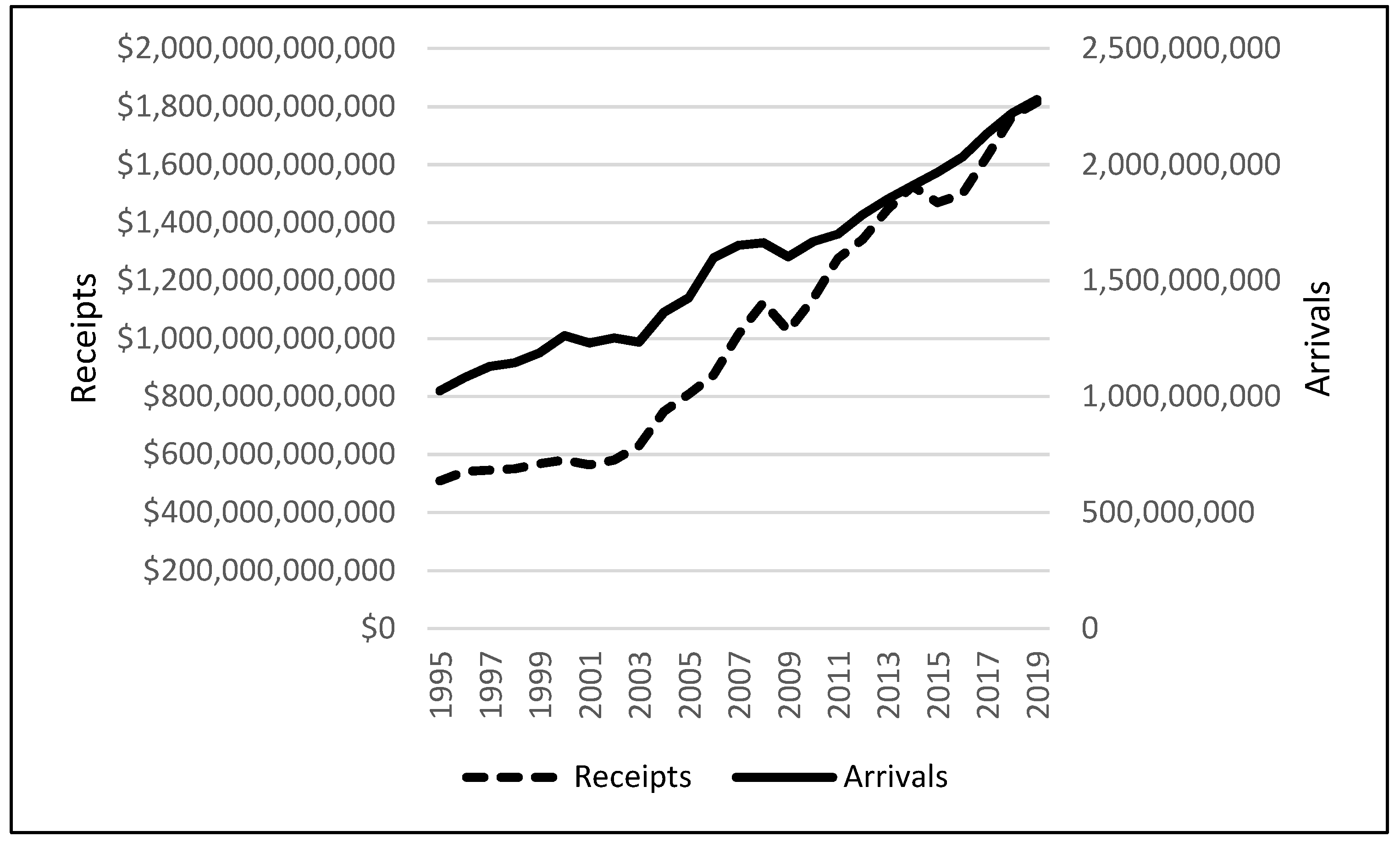
According to the 2020 report of UNWTO, tourism has greatly benefited from the rapid pace of globalization. It represents one of the top five export categories for over 80 percent of countries. Tourism is also the primary source of foreign exchange earnings for up to 40 percent of the world’s economies while supporting one in ten jobs worldwide. Between 2009 and 2019, real growth in international tourism receipts (54%) exceeded growth in global GDP (44%). The report further shows that total tourist arrivals in 2019 reached a new high of almost 2.3 billion, a three percent increase from the year before. At the same time, tourism earnings increased to a record $1.8 trillion, which was also three percent higher than the year before. The 2020 report also shows that leisure travel is preeminent. Its share of worldwide tourism grew from 50 percent in 2000 to 56 percent in 2018.

Figure 1 shows the multiyear growth in global tourist arrivals and tourism receipts. Barring the hiccup that occurred during the 2008 Global Financial Crisis and the devastating impact of the 2020–2021 COVID-19 pandemic, the persistent uptrend in tourism demand, measured by arrivals and receipts, is unmistakable.

In its 2018 visa facilitation report, the UNWTO identified the contributing factors to the surge in international tourism. These include the growing strength of the global economy; a rising middle class, especially in the developing economies; technological advances that facilitate travel arrangements and enhance vacation experience; affordable travel costs; and visa facilitation. The last factor is particularly noteworthy. It reflects a growing trend by many countries to switch from standard tourist visa requirements to the convenience of visa-free entry, eVisa, or visa on arrival. Consequently, the UNWTO 2018 report showed that the share of countries requiring traditional tourist visas declined from 75 percent in 1980 to about 50 percent in 2018.

Recent tourism trends show that Europe and the Middle East enjoy the highest growth in arrivals as well as in tourism earnings (UNWTO 2021). Europe’s year-over-year growth rate in real terms was four percent. It was eight percent for the Middle East. France and Spain compete for the number one position in tourist arrivals. The United States ranked a close third with about 80 million inbound tourists. However, the U.S. ranks a distant first in terms of tourism earnings, which grew to a record $214 billion in 2019, accounting for more than nine percent of total U.S. exports for that year. According to the U.S. Travel Association (Travel Facts and Figures 2020), one-half of all inbound tourists are from Canada and Mexico. The leading inbound tourists from outside North America are from the United Kingdom, Japan, China, and South Korea, in that order.

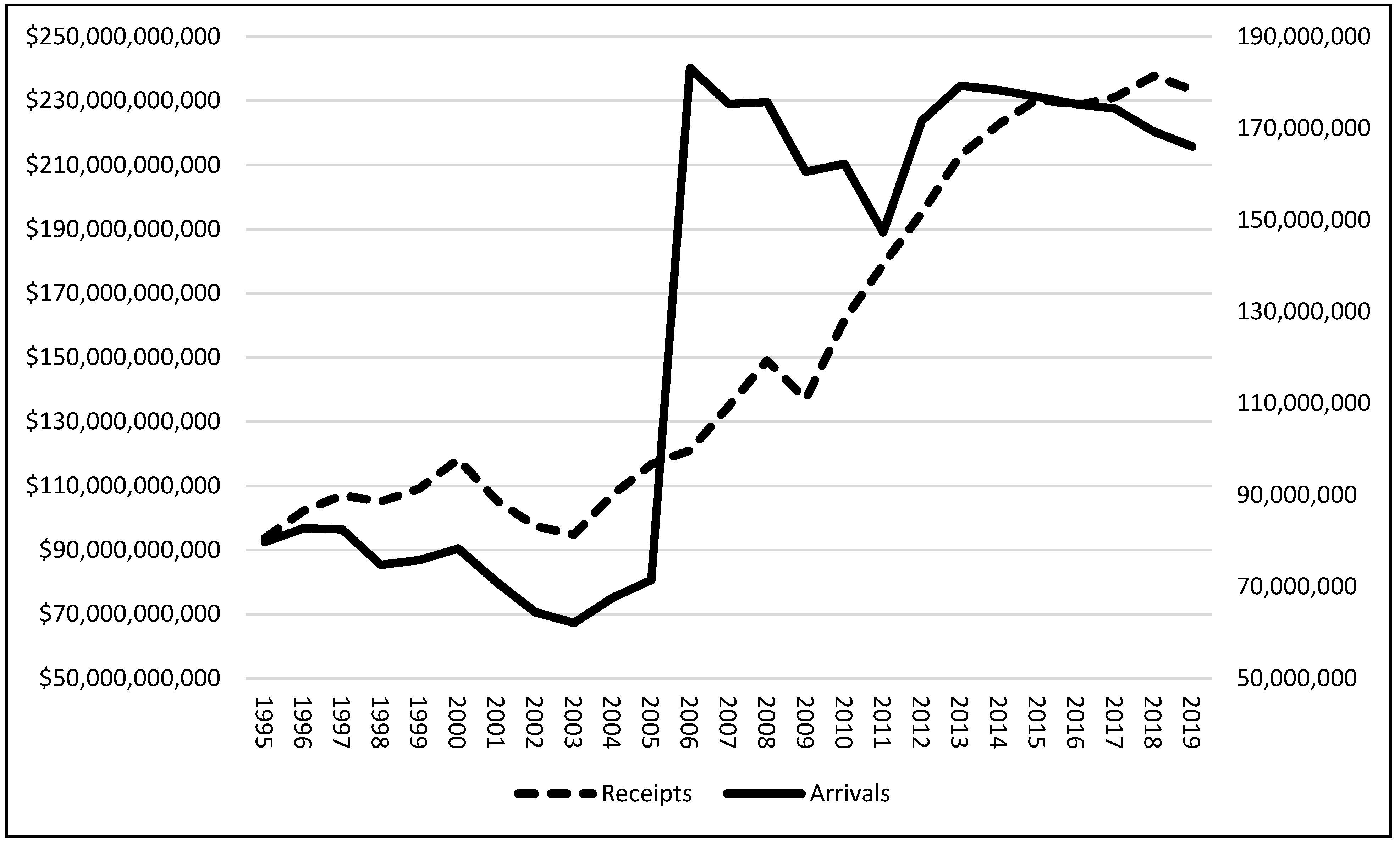
Figure 2 shows the recent trend in U.S. tourism. Similar to the global trend in Figure 1, the U.S. has continued to enjoy steady growth in both arrivals and receipts, especially in periods outside of the economic shocks of the 9/11 attack, the 2008–2009 financial crisis, and the 2020–2021 COVID pandemic. The extent to which such risks impact tourism has been extensively examined in the literature, more recently by Khalid et al. (2019) in a panel dataset of 200 countries.

Currency valuation has been cited as an additional factor influencing a tourist’s choice of destination, especially for leisure purposes (Obi et al. 2016, Yap 2012). To that end, the World Travel and Tourism Council (WTTC) points out that one critical way of capturing the impact of the exchange rate is to measure a destination’s currency against the currency of that destination’s visitor markets. It argues that such a visitor-weighted exchange rate should reveal the direct impact of the exchange rate on tourism trends (World Travel & Tourism Council, 17 August 2016).1 To account for this factor, this study incorporates currency valuation in addition to market risk in developing a tourism-growth model. Tourism development is measured by tourist arrivals, while economic growth is measured by real gross domestic product. The interrelationships between these variables are investigated using the recently developed autoregressive distributed lag (ARDL) cointegration technique developed by Pesaran et al. (2001) and extended by Shin et al. (2014) using an asymmetric framework. The model’s strength lies in its ability to incorporate both stationary and nonstationary regressors in the examination of short-run and long-run dynamics between the variables.

The rest of this study is as follows: Section 2 summarizes recent literature that addresses different tourism-growth hypotheses. Following that is a description of the data and estimation model. Empirical results and conclusions are presented in Section 4 and Section 5, respectively. A discussion of economic and policy implications is provided in the final section.

2. Literature

The literature offers three principal views on the relationship between tourism development and economic growth. The first, referred to as tourism-led growth, argues that tourism development drives economic growth. The second is growth-led tourism, which states that economic growth drives tourism development. The third view is a hybrid and asserts that economic growth and tourism development drive each other. In effect, it argues that a bidirectional causality exists between the two variables. Recent studies that provide a review of the tourism-growth literature include Brida and Pulina (2010), Pablo-Romero and Molina (2013), and Gwenhure and Odhiambo (2016).

Pablo-Romero and Molina (2013) point out that the relationship between tourism and growth depends on various factors, the main one being the country’s degree of specialization in tourism. They also show that empirical results are sensitive to variable specifications and the modeling technique used. Also, Gwenhure and Odhiambo (2016) show that the causal effects between tourism and growth differ from country to country and, similar to Pablo-Romero and Molina’s observations, depend on the methodology used. On balance, both studies find that the weight of empirical evidence leans toward the tourism-led growth hypothesis.

The tourism-led growth view is consistent with the position of both the United Nations World Travel Organization (UNWTO) and the World Travel and Tourism Council (WTTC). Both of these institutions provide data documenting the employment and income benefits of international tourism. Many studies have shown direct evidence linking tourism with growth in the world. Examples include Antonakakis et al. (2015) for Europe, Odhiambo (2011, 2012) for sub-Saharan African economies, Pratt (2015) for the Caribbean and Pacific Island states, Brida et al. (2015) for South American countries, Isik et al. (2018) for China and Turkey, and Stylianou et al. (2019) for a group of other Asian countries.

One of the most comprehensive studies on tourism-led growth is by Tang and Tan (2017). They investigated the validity of this hypothesis for 167 countries. After accounting for differences in the levels of income and governance, they found evidence in support of the hypothesis, observing that the effect of tourism on growth is contingent on the level of income and institutional qualities of the host country. In a similar panel study of European and Asian countries, Stylianou et al. (2019) found evidence of unidirectional causality from tourism to economic growth. Manzoor et al. (2019) investigated the impact of tourism on Pakistan’s economic growth and employment. They found that economic growth and employment respond positively to tourism development in the long run. Pratt (2015) compared tourism’s economic impact for seven small island development states, the so-called SIDS. They found that tourism generates a large amount of economic activity. However, the income that remains in the host countries is often a fraction of the actual money spent by tourists. In addition to the direct economic benefits, Zurub et al. (2015) explained that tourism leads to sustainable economic development in many European Union states, especially the emerging economies of Eastern Europe.

The literature on growth-led tourism shows that tourists are attracted to a destination if the right infrastructure is already in place. Evidence that supports this view includes Ging and Lee (2008) in the case of Singapore, Payne and Mervar (2010) for Croatia, and Katircioglu (2009) for the Mediterranean island nation of Cyprus. More recent studies include Isik et al. (2018) in Spain and Aratuo and Etienne (2018) for a specific U.S. case. The study by Aratuo and Etienne was set against the U.S. lodging and entertainment sectors. They investigated the relationship between economic growth and the following tourism sectors in 1998–2017: accommodation, air transportation, shopping, food and beverage, recreation, and entertainment. They found no evidence of a long-run relationship between any of these tourism sectors and growth. However, in the short run, they found a unidirectional causality from economic growth to tourism demand.

Recent studies showing evidence of bidirectional causality include Seghir et al. (2015), Antonakakis et al. (2015), Lin et al. (2018), Isik et al. (2018), and Stylianou et al. (2019). In a panel cointegration and causality test, Seghir et al. (2015) examined the relationship between tourism spending and economic growth for 49 countries in 1988–2012. Their results show cointegration between the two variables and a two-way causality for the pooled dataset. In a similar study, Lin et al. (2018) found that less-developed economic regions covering larger geographic areas in China are more likely to experience tourism-led growth. However, other regions that are less-developed but smaller are more disposed to the benefits of growth-led tourism. Both Antonakakis et al. (2015) and Stylianou et al. (2019) found evidence of bidirectional causality for European countries. However, as Antonakakis et al. (2015) observed, the relationship appears to be unstable over time regarding both the magnitude and direction of causality. Separately, Isik et al. (2018) found evidence of bidirectional causality in Europe’s largest economy, Germany. However, this is only when renewable energy consumption is included in the framework as a mediating factor.

Other mediating variables featured in recent tourism studies include market risk, the exchange rate, and trade. The issue of terrorism risk was recently considered by Fareed et al. (2018). Using the novel asymmetric cointegration approach developed by Shin et al. (2014), they found that in the case of Thailand, the response of economic growth to tourism development is significantly hindered by the risk of terrorism. Khalid et al. (2019) investigated the mediating effects of other risk factors, including inflation, stock market crash, and financial crisis. Their study, which utilized a panel dataset of 200 countries over 1995–2010, reveals that inflation crises dampen international tourism flows in both the destination and origin countries. They also find that domestic debt crises encourage international tourism arrivals, perhaps because of the host country’s currency devaluation at such times. Similarly, Obi et al. (2016) showed that a weak domestic currency enhances tourism benefits by boosting dollar-denominated tourism earnings.

Kibara et al. (2012) used the ARDL-bounds testing approach to examine the Kenyan tourism sector’s growth impact by incorporating trade as a mediator. They found a unidirectional causality from tourism to economic growth in both the short and long run. They found, moreover, that international tourism Granger-causes trade while trade Granger-causes economic growth. Obi et al. (2015) used implied volatility as a proxy for systematic risk in examining U.S. tourism stocks’ dynamics. They found that volatility has a negative causal effect on tourism stocks in the long run, but not in the short run. Tourism stocks, on the other hand, have only a short-run causal impact on implied volatility. Upon reaching this finding, the authors concluded that the tourism industry, which is often at the frontline of global shocks such as COVID-19 in 2020, is crucial for near-term volatility in the equity market., Khalid et al. (2019) showed that during times of banking crises the North American tourism industry is often more adversely affected than other nonbank related sectors.

A recent tourism study of specific interest is by Isik et al. (2018). They tested the relationship between economic growth on the one hand, and tourism development and renewable energy consumption on the other, using a pooled sample from the following seven countries: China, France, Germany, Italy, Spain, Turkey, and the United States. Their study period was from 1995 to 2012. Similar to this study, tourism development was measured by tourist arrivals. Their empirical results for the entire panel of seven countries showed a one-way causality running from tourist arrivals to economic growth, supporting the tourism-led growth hypothesis. However, when examined in isolation, there was no evidence of a causal relationship between these two variables in the case of the United States. Nevertheless, for the U.S., there is evidence of causality from energy to growth, and separately, from tourism to energy.

This study adds to the existing literature in three important ways. First, unlike studies that examine the individual economic impact of tourism development, energy, risk, and the exchange rate as summarized in this section, this study introduces the last two factors as mediators within a multivariate tourism-growth framework. It allows us to examine the transmission mechanism through which growth and tourism may be related. This approach is guided by findings in studies demonstrating that individually, risk and currency valuation are linked to tourism demand. Second, this study utilizes the recently developed ARDL cointegration approach together with its nonlinear variant, NARDL, to examine short- and long-run relationships among the variables. This enables us to overcome the modeling challenges pointed out by Gwenhure and Odhiambo (2016), Nkoro and Uko (2016), and Pablo-Romero and Molina (2013). Third, it is the first of such studies to ascertain the tourism-growth question solely for the U.S., the largest tourism destination in terms of tourism earnings.

3. Data and Methodology

The prime purpose of this study is to examine whether causal linkages exist between tourism development and economic growth in the United States. The impact of currency valuation and risk in the tourist’s decision to travel to the U.S. is incorporated in the model. Accordingly, the initial research question is: Does the tourism-growth relationship holds for the U.S. as it does for most other economies? Second: Does implied volatility, together with currency valuation, influence the tourism-growth relationship?

Quarterly data for the following variables were used in the empirical analysis: real gross domestic product (GDP), tourist arrivals (TA), implied volatility (IV), and nominal effective exchange rate (FX). The GDP variable measures economic growth, while tourist arrival measures tourism demand. Studies utilizing similar proxies include Isik et al. (2018), Brida et al. (2015), and Tang et al. (2016). Implied volatility (IV), measured by the Chicago Board Options Exchange (CBOE) volatility index called VIX, is a measure of expected market volatility. The nominal effective exchange rate, measured for the U.S. dollar, captures the impact of currency valuation on tourism demand. Including the exchange rate variable in the model is particularly salient to this study. Pursuant to WTTC’s view, one critical way of capturing the direct impact of the exchange rate on tourism is to measure a destination’s currency against the currency of that country’s primary visitor markets. To that end, NEER, a weighted average rate at which the dollar exchanges for a basket of multiple foreign currencies, was utilized in the analysis.

Data for GDP and exchange rate were obtained from the Federal Reserve Bank of St. Louis. Tourism data came from multiple sources, including the United Nations World Tourism Organization (UNWTO) and World Bank Development Indicators (WBDI). Sample data were obtained from Q1-1996 to Q2-2019, which is the most extended period in which complete data were available for all the variables.

The ARDL Cointegration Approach

This study’s initial unrestricted error correction model is the autoregressive distributed lag (ARDL) bounds testing technique. This estimator, which was popularized by Pesaran and Shin (1999) and Pesaran et al. (2001), has become the gateway for determining the existence of a dynamic relationship between stationary and nonstationary time series. It also enables the reparameterization of the variables to the error correction model (ECM). The following ARDL models were used to test the principal variables’ dynamic linkages:

$$\begin{gathered} \Delta \ln (GD{P}_t)={\beta }_0+{\displaystyle \sum }_{i=1}^{p-1}{\lambda }_i\Delta \ln (GD{P}_{t-i})+{\displaystyle \sum }_{i=0}^{q-1}{\delta }_i\Delta \ln (T{A}_{t-i}) \\ +{\phi }_{1}ln(GD{P}_{t-1})+{\phi }_{2}ln(T{A}_{t-1})+{\upsilon }_t \end{gathered}$$

(1)

$$\begin{gathered} \Delta \ln (T{A}_t)={\beta }_0+{\displaystyle \sum }_{i=1}^{p-1}{\lambda }_i\Delta \ln (T{A}_{t-i})+{\displaystyle \sum }_{i=0}^{q-1}{\delta }_i\Delta \ln (GD{P}_{t-i}) \\ +{\phi }_{1}ln(T{A}_{t-1})+{\phi }_{2}ln(GD{P}_{t-1})+{\upsilon }_t \end{gathered}$$

(2)

where GDP is the seasonally adjusted real gross domestic product, TA is the tourism development metric defined as tourist arrivals; and ν_t is the iid innovation term. The short-run coefficients of the model are λ_i and δ_i, while the long-run coefficients are φ₁ and φ₂. Inclusion of the mediating variables extends Equations (1) and (2) to the following functional forms:

$$GDP=f\left(TA, IV, FX\right)$$

$$TA=f\left(GDP, IV, FX\right)$$

where IV and FX are the two mediating regressors. Similar to the error correction model (ECM) of Engle and Granger (1987), ARDL models are symmetric time series models in which both the dependent and independent variables are related not only contemporaneously but across historical (lagged) values. However, unlike the traditional ECM, the ARDL approach can be specified for regressors of I(1) and I(0) but not higher. Therefore, outside of the need to ensure that none of the variables is I(2) or higher, use of the ARDL method does not necessarily require pretests for unit root as with traditional error correction models. Also, the ARDL model is an unrestricted ECM because all the long-run terms are individually specified and not restricted with a single error correction term.

One limitation of the ARDL is that it assumes linearity so that positive and negative shocks to the regressors are assumed to have the same level of effect on the target variable. As a resolution, the symmetric ARDL bounds test described above is supplemented with its asymmetric equivalent, the nonlinear autoregressive distributed lag (NARDL). The NARDL model, which was popularized by Shin et al. (2014), offers a path for decomposing the regressors into positive and negative shocks. This allows one to ascertain if the response variable reacts differently to the explanatory variables’ positive and negative shocks. The bivariate formulation of the NARDL for the primary variables in the model (GDP and TA) is presented in Equations (3) and (4).

$$\begin{gathered} \Delta ln(GD{P}_t)={\beta }_0+{\displaystyle \sum }_{i=1}^{p-1}{\lambda }_i\Delta ln(GD{P}_{t-i})+{\displaystyle \sum }_{i=0}^{q-1}{\delta }_{1i}\Delta \ln \left(T{A}_{t-i}^{+}\right)+{\displaystyle \sum }_{i=0}^{q-1}{\delta }_{2i}\Delta ln\left(T{A}_{t-i}^{-}\right) \\ +\rho ln(GD{P}_{t-1})+{\phi }^{+}ln(T{A}_{t-1}^{+})+{\phi }^{-}ln(T{A}_{t-1}^{-})+{\upsilon }_t \end{gathered}$$

(3)

$$\begin{gathered} \Delta ln(T{A}_t)={\beta }_0+{{\displaystyle \sum }}_{i=1}^{p-1}{\lambda }_i\Delta ln(T{A}_{t-i})+{{\displaystyle \sum }}_{i=0}^{q-1}{\delta }_{1i}\Delta ln\left(GD{P}_{t-i}^{+}\right)+{{\displaystyle \sum }}_{i=0}^{q-1}{\delta }_{2i}\Delta ln\left(GD{P}_{t-i}^{-}\right) \\ +\rho ln(T{A}_{t-1})+{\phi }^{+}ln(GD{P}_{t-1}^{+})+{\phi }^{-}ln(GD{P}_{t-1}^{-})+{\upsilon }_t \end{gathered}$$

(4)

where TA⁺, TA⁻, GDP⁺, and GDP⁻ represent partial cumulative sums of positive and negative changes in the regressors. The asymmetric short-run coefficients are δ₁ and δ₂, while those for long-run asymmetry are φ⁺ and φ⁻. Using the Wald test, a rejection of the null hypothesis of symmetry leads to the conclusion that the magnitude of changes in the target variable when the regressor increases are not the same as when it decreases.

To test the existence of asymmetric long-run cointegration, Shin et al. (2014) proposed the bounds test, a joint test of all the lagged levels of the regressors. Two tests of significance that serve this purpose are the t-statistic of Banerjee et al. (1998) and the F-statistic of Pesaran et al. (2001). The t-statistic tests the null hypothesis φ = 0 against the alternative hypothesis φ < 0. The F-statistic tests the null hypothesis φ = φ⁺ = φ⁻ = 0. If we reject the null hypothesis of no cointegration, we conclude that a long-run relationship exists among the variables. The long-run asymmetric coefficients are estimated as

$$L_{M1+}=\frac{-{\phi }^{+}}{\rho } and L_{M1-}=\frac{-{\phi }^{-}}{\rho }$$

Using the Wald test, the following null hypotheses for long-run and short-run asymmetries are tested:

$$\mathrm{Long}\mathrm{run}{\mathrm{H}}_0:\frac{-{\phi }^{+}}{\rho }=\frac{-{\phi }^{-}}{\rho }$$

$$\mathrm{Short}\mathrm{run}{\mathrm{H}}_0:{{\displaystyle \sum }}_{i=0}^{q-1}{\delta }_i^{+}={{\displaystyle \sum }}_{i=0}^{q-1}{\delta }_i^{-}$$

A rejection of any of these hypotheses leads to the conclusion that the impact of the regressor on the target variable is asymmetric in either the long run or the short run, whichever is the case.

This approach of supplementing a linear ARDL inquiry with NARDL was also employed by Rocher (2017) and Isik et al. (2018). As highlighted by Rocher (2017), an essential benefit of this extension is the ability to test for hidden cointegration and differentiate among linear cointegration, nonlinear cointegration, and lack of cointegration. Hidden cointegration is when no cointegration is detected using symmetric models but is found between positive and negative components of the series (Granger and Yoon 2002).

4. Results

Results of the descriptive statistics of the variables are presented in

Table 1. Descriptive statistics.

	GDP	TA	FX	IV
Mean	15,082	13,540,178	87.16	20.16
Median	15,342	12,308,982	87.22	18.22
Mode	#N/A	#N/A	#N/A	13.29
Standard Deviation	2136	4,317,131	10.75	7.63
Kurtosis	−0.7839	−0.9586	−0.6895	1.6702
Skewness	−0.1410	0.4866	0.2652	1.3052
Minimum	10,818	6,834,658	69.09	9.51
Maximum	19,023	22,562,970	111.38	44.14
Sample size	94	94	94	94

GDP = real GDP in billions of USD (sample period: Q1, 1996–Q2, 2019): TA = international tourist arrivals, measured in thousands; FX = nominal effective exchange rate for US dollar; IV = CBOE volatility index.

. Over the sample period, the highest GDP level was $19 trillion. The lowest was $10.82 trillion. The highest and lowest values for tourist arrivals were 22.56 million and 6.83 million, respectively. The first evidence that none of the series is normally distributed is the lack of uniformity of the three measures of central tendency: mean, median, and mode. Also, all the series except GDP are positively skewed, indicating that the distribution’s mass is concentrated on the left. Thus, one is more likely to find low values more frequently than high values. This negative skew of GDP reflects the phenomenal growth of the US economy during the dot com period and after the 2008 financial crisis.

Except for volatility, all the variables have negative excess kurtosis. This so-called platykurtic behavior means that the frequency distribution has thinner tails and is flatter than the normal distribution. A negative excess kurtosis also implies that the distribution’s outlier character is less extreme than that of a normal distribution. To be sure, these kurtosis values are relative kurtosis and were calculated relative to the absolute kurtosis of the normal distribution, which is 3.

Unit root test results are summarized in

Table 2. Unit root test.

Time Series	Level		1st Difference
	t-Stat	p-Value	t-Stat	p-Value
GDP	−1.8607	0.3494	−4.1969 ***	0.0011
TA	−0.4155	0.9010	−4.3923 ***	0.0006
FX	−1.2930	0.6302	−8.5636 ***	0.0000
IV	−4.3659 ***	0.0006

Null hypothesis: Series has unit root (non-stationary); *** Significant at α = 0.01; GDP = real GDP; TA = tourist arrivals; FX = nominal effective exchange rate (USD); IV = CBOE volatility index. All variables in natural logarithm.

. Ordinarily, stationarity tests are not necessary for ARDL or NARDL modeling except to ensure that none of the variables are I(2) or higher. Both cointegration models permit the inclusion of I(0) and I(1) regressors.

The Augmented Dickey–Fuller (ADF) unit root test was initially performed on each of the series. However, given the low power of the ADF test pointed out by West (1988), stationarity tests were supplemented by Phillips–Perron, Dickey–Fuller GLS, and Ng–Perron. Results of these other stationarity tests were consistent with those of the ADF results, each producing a negative coefficient to ensure the estimation model’s validity. In all cases, except for IV which is stationary at level, all the variables are stationary in their first differences. The finding that some regressors are stationary at level, while others are stationary in their first differences, necessitates using the bounds testing approach.

Table 3. Preliminary ARDL bounds test result.

Dependent	Regressor	F	I(0)	I(1)	ECTt-1	p-Value
GDP	TA	2.61	4.94	5.73	NA	NA
TA	GDP	2.61	4.94	5.73	NA	NA

GDP = real GDP; TA = tourist arrivals. Estimation equations: $\Delta ln(GD{P}_t)={\beta }_0{{\displaystyle \sum }}_{i=1}^{p-1}{\lambda }_i\Delta ln(GD{P}_{t-i})+{{\displaystyle \sum }}_{i=0}^{q-1}{\delta }_i\Delta ln(T{A}_{t-i})+{\phi }_{1}ln(GD{P}_{t-1})+{\phi }_{2}ln(T{A}_{t-1})+{\upsilon }_t;$ $\Delta ln(T{A}_t)={\beta }_0+{{\displaystyle \sum }}_{i=1}^{p-1}{\lambda }_i\Delta ln(T{A}_{t-i})+{{\displaystyle \sum }}_{i=0}^{q-1}{\delta }_i\Delta ln(GD{P}_{t-i})+{\phi }_{1}ln(T{A}_{t-1})+{\phi }_{2}ln(GD{P}_{t-1})+{\upsilon }_t$.

presents the initial results of the ARDL bounds test. According to Pesaran et al. (2001), cointegration exists if the calculated F statistic is greater than the upper bound, I(1). There is no cointegration if F is below the lower bound, I(0). Results that fall between the upper and lower bounds are indeterminate. The results shown here are for the bivariate case defined in Equations (1) and (2) for GDP and TA. As can be seen, in both cases, the F statistic is less than I(0), indicating there is no evidence of cointegration between growth and tourism. Without cointegration, the need to specify the error correction mechanism no longer exists.

The absence of a long-run relationship between tourism and growth for the U.S. is arguably counterintuitive for three critical reasons. The first is that tourism earnings are a significant portion of U.S. export earnings and a third of service exports2. Second, among the top tourism earners, the U.S. consistently ranks on top, boasting the world’s largest international tourism surplus of over $60 billion in 2019 alone (UNWTO 2021). The UNWTO 2020 report also showed that in 2019, the U.S. earned over $214 billion from tourism, which is larger than the total receipts of the next three earners (France, Spain, and Thailand) combined. Further, the U.S. consistently ranks in the top three in terms of tourist arrivals, after France and Spain. Finally, tourism development is widely documented as playing a crucial role in economic growth (Isik et al. 2018; Manzoor et al. 2019; Pablo-Romero and Molina 2013). However, although tourism constitutes a significant portion of the service sector for the U.S., the sheer size and diverse nature of the country’s economy potentially crowd out its significance except when direct factors driving inbound tourism are examined in concert. As outlined by Obi et al. (2015), these factors include currency valuation and risk. These findings motivate the inclusion of implied volatility and the exchange rate as mediating factors within a multivariate error correction framework.

Arguably, a weak domestic currency increases a country’s desirability as a tourism destination, other factors considered. Inbound tourists get more value for their travel budget if their national currencies are strong relative to the U.S. dollar. Obi et al. (2016) successfully demonstrated that one important way to capture the impact of risk on tourism development is to examine the relationship between implied volatility and tourism receipts. The benefit of this approach is that implied volatility, which captures investor fear in the equity market, rises with risk and decreases when risk ebbs. As it turns out, when these two variables are included in the model, a cointegration is readily achieved between growth and tourism. The results are presented in

Table 4. ARDL bounds test of cointegration with mediating variables +.

Dependent	Regressor	F	I(0)	I(1)	ECTt−1	p-Value
GDP	TA	8.15 ***	4.29	5.61	−0.0307	0.0000
TA	GDP	18.11 ***	4.29	5.61	−0.1106	0.0000

+ GDP = real GDP; TA = tourist arrivals; Mediating variables: exchange rate (FX) and implied volatility (IV); *** Significant at α = 0.01; Estimation equations: $\Delta ln(GD{P}_t)={\beta }_0{{\displaystyle \sum }}_{i=1}^{p-1}{\lambda }_i\Delta ln(GD{P}_{t-i})+{{\displaystyle \sum }}_{i=0}^{q-1}{\delta }_{1i}\Delta ln(T{A}_{t-i})+{{\displaystyle \sum }}_{i=0}^{q-1}{\delta }_{2i}\Delta ln(F{X}_{t-i})+{{\displaystyle \sum }}_{i=0}^{q-1}{\delta }_{3i}\Delta ln(I{V}_{t-i})+{\phi }_{1}ln(GD{P}_{t-1})+{\phi }_{2}ln(T{A}_{t-1})+{\phi }_{3}ln(F{X}_{t-1})+{\phi }_{4}ln(I{V}_{t-1})+{\upsilon }_t;$ $\Delta ln(T{A}_t)={\beta }_0{{\displaystyle \sum }}_{i=1}^{p-1}{\lambda }_i\Delta ln(T{A}_{t-i})+{{\displaystyle \sum }}_{i=0}^{q-1}{\delta }_{1i}\Delta ln(GD{P}_{t-i})+{{\displaystyle \sum }}_{i=0}^{q-1}{\delta }_{2i}\Delta ln(F{X}_{t-i})+{{\displaystyle \sum }}_{i=0}^{q-1}{\delta }_{3i}\Delta ln(I{V}_{t-i})+{\phi }_{1}ln(T{A}_{t-1})+{\phi }_{2}ln(GD{P}_{t-1})+{\phi }_{3}ln(F{X}_{t-1})+{\phi }_{4}ln(I{V}_{t-1})+{\upsilon }_t$.

. The bounds test confirms cointegration at any conventional level of significance. In both cases, the F statistic is greater than the upper bound critical value of 5.61.

With cointegration confirmed, the next step is to examine the error correction mechanism. Results of the test of significance for the error-correction term (ECT) are shown in the last two columns of Table 4 for the cointegrated series. In both cases, the speed of adjustment, which is the ECT coefficient, is statistically significant with the correct (negative) sign. When the target variable is GDP, about 0.03 percent of departures from equilibrium are corrected each period. About 0.11 percent of departures from equilibrium are corrected each period when tourism is the target variable. Because of the cointegration in both equations, one can also conclude that a bidirectional Granger causality exists between GDP and tourism development when risk and currency valuation are considered. A causal link between tourism development and economic growth supports the tourism-led growth hypothesis (Lee and Brahmasrene, 2013; Tang et al. 2016; Isik et al. 2018) by suggesting that increases in tourism demand improve the overall economy. It also confirms the existence of growth-led tourism based on bidirectional causality.

Results of the long-run levels equation are summarized in

Table 5. Long-Run Levels Symmetric Test Result.

Target Variable: GDP
Variable	Coefficient	t-Statistic	p-Value
TA	0.2723 ***	4.7720	0.0000
IV	−0.2575 ***	−4.4700	0.0000
FX	0.1583	1.0264	0.3077
Target Variable: TA
Variable	Coefficient	t-Statistic	p-Value
GDP	2.2732 ***	3.5639	0.0006
IV	0.2980	1.2413	0.2183
FX	−4.1942 **	−2.2508	0.0273

*** Significant at α = 0.01; ** Significant at α = 0.05. GDP = real GDP; TA = tourist arrivals; IV = implied volatility; FX = exchange rate. All variables in natural logarithm. Long-run levels equation is the cointegrating equation represented in the error correction model by the error correction term and defined as: $ln\left(GD{P}_t\right)={\beta }_0+{\beta }_{1}ln\left(T{A}_t\right)+{\beta }_{2}ln\left(I{V}_t\right)+{\beta }_{3}ln\left(F{X}_t\right)+{ϵ}_t$; $ln\left(T{A}_t\right)={\beta }_0+{\beta }_{1}ln\left(GD{P}_t\right)+{\beta }_{2}ln\left(I{V}_t\right)+{\beta }_{3}ln\left(F{X}_t\right)+{ϵ}_t$.

. The top part is the case in which GDP is the target variable. As expected, tourism development positively impacts economic growth, while volatility (IV) has a negative impact. These results show that a one percent increase in tourist arrivals increases real GDP by about 0.27 percent in the long run. This causal effect is statistically significant at the 1 percent level.

The second half of Table 5 shows the long-run levels’ results when tourism is the target variable. We find that both real GDP and the exchange rate coefficients are statistically significant. Specifically, a one percent increase in real GDP leads to a 2.27 percent increase in tourist arrivals. Also, a one percent increase in the dollar’s value leads to a 4.19 percent decrease in tourist arrivals. Both outcomes are statistically significant at the 0.05 level.

The finding on currency valuation supports the view that a weak dollar encourages foreign visitors, especially those traveling on a budget. Notwithstanding these results, and as Shin et al. (2014) observed, if asymmetry exists between the variables, these inferences, which are based on the symmetric ARDL model, may be less informing. Therefore, and similar to the approach employed by Rocher (2017) and Isik et al. (2018), we supplement the preceding analysis with the NARDL bounds test as specified in Equation (3). This allows us to determine if GDP and tourism have a nonlinear relationship when volatility and exchange rate are considered. Results of the long-run levels asymmetric bounds test are summarized in

Table 6. Long-run levels asymmetric test result.

Target Variable: GDP
	Coefficient	t-Statistic	p-Value
TA_POS	0.1318 **	2.4043	0.0186
TA_NEG	0.0044	0.0761	0.9395
IV_POS	−0.1432 ***	−3.3933	0.0011
IV_NEG	−0.1549 ***	−2.9747	0.0039
FX_POS	−0.2510	−1.3293	0.1876
FX_NEG	0.3542 *	1.8235	0.0721
F statistic + 6.10 ***
Target Variable: TA
GDP_POS	2.4712	1.0609	0.2926
GDP_NEG	−11.2067 **	−2.1218	0.0376
IV_POS	0.1743	1.1162	0.2684
IV_NEG	0.4624 **	2.0744	0.0419
FX_POS	−0.4710	−0.5125	0.6100
FX_NEG	−1.8704 *	−1.6482	0.0941
F statistic + 14.26 ***

*** Significant at α = 0.01; ** Significant at α = 0.05; * Significant at α = 0.10; + Critical value at 1% for I(1) = 3.99; GDP = real GDP; TA = tourist arrivals; IV = CBOE implied volatility; FX = exchange rate. All variables in natural logarithm. Long-run asymmetric levels equation is the cointegrating equation represented in the error correction model by the error correction term and defined as: $ln\left(GD{P}_t\right)={\beta }_0+{\beta }_1^{+}ln(T{A}_t^{+})+{\beta }_1^{-}ln(T{A}_t^{-})+{\beta }_2^{+}ln(I{V}_t^{+})+{\beta }_2^{-}ln(I{V}_t^{-})+{\beta }_3^{+}ln(F{X}_t^{+})+{\beta }_3^{-}ln(F{X}_t^{-})+{ϵ}_t$; $ln\left(T{A}_t\right)={\beta }_0+{\beta }_1^{+}ln(GD{P}_t^{+})+{\beta }_1^{-}ln(GD{P}_t^{-})+{\beta }_2^{+}ln(I{V}_t^{+})+{\beta }_2^{-}ln(I{V}_t^{-})+{\beta }_3^{+}ln(F{X}_t^{+})+{\beta }_3^{-}ln(F{X}_t^{-})+{ϵ}_t$.

.

The top part of the table is the case in which GDP is the target variable. Interestingly, only positive shocks in tourism development are directly linked to GDP growth; negative shocks have no effect. A one percent increase in tourist arrivals generates a 0.13 percent increase in real GDP in the long run. Thus, while the tourism-led growth hypothesis is still upheld when asymmetry is considered, that only happens when improvements in tourism are in effect. Declines in tourism development have no causal effect, perhaps due to the diversified nature of the economy.

Although weakly significant, negative shocks in the exchange rate, Granger causes economic growth in the long run. A one percent decline in the exchange rate (FX_NEG) leads to 0.35 percent decline in real GDP. This is probably because a weaker dollar encourages increased foreign direct investments, makes American goods more competitive overseas, and in this case, also makes visiting the US more attractive. This last observation is underscored by the negative coefficient of −1.87 for negative shocks to the exchange rate (FX_NEG) in the second part of Table 6.

With tourism as the target variable, we find that only negative shocks to GDP affect tourism; positive shocks have no causal effect. Negative shocks in GDP have an inverse effect on U.S. tourism. In other words, economic downturns increase international tourism in the long run. Specifically, a one percent decline in real GDP causes inbound tourism to rise by 11 percent. This outcome, which differs from the positive impact suggested by the symmetric model, reinforces the distinct benefit of examining asymmetries in error correction models, as Shin et al. (2014) point out.

The inverse relationship between tourism and negative shocks in GDP may initially seem counterintuitive. However, it can be linked to the relationship between tourism and the exchange rate. As can be seen, negative shocks to both GDP and the exchange rate lead to improvements in tourism development. In other words, tourism rises with declines in GDP (negative coefficient of −11.2) and value of the dollar (negative coefficient of −1.8704). Thus, the currency’s value delineates the inverse relationship between rise in tourism and weak economy. A one percent drop in the dollar’s value leads to a 1.87 percent rise in tourism. Correspondingly, a one percent drop in the dollar’s value leads to a 0.35 percent decline in real GDP, which is associated with a rise in inbound tourism. This outcome points to the fact that while growth-led tourism is also supported in the case of the United States, it is only supported when economic declines are accompanied by a weak dollar, both of which make visiting the U.S. a bargain especially for inbound tourists on a budget.

Short Run Causality and Model Diagnostics

Short run causality test results, summarized in

Table 7. Short-run asymmetric causality test results.

Target Variable: TA
Variable	Coefficient	t-Statistic	Prob.
D(GDP_POS)	1.9411	1.0848	0.2820
D(GDP_POS(-1))	2.4884	1.5380	0.1288
D(GDP_POS(-2))	4.3179 ***	2.7063	0.0087
D(GDP_POS(-3))	4.3976 ***	2.7800	0.0071
D(GDP_NEG)	2.1514	0.6538	0.5155
D(GDP_NEG(-1))	13.8278 ***	4.1046	0.0001
D(GDP_NEG(-2))	−0.8973	−0.2637	0.7928
D(GDP_NEG(-3))	9.4231 ***	2.8622	0.0056
Wald test +		4.2979 **	0.0382

*** Significant at α = 0.01; ** Significant at α = 0.05; + Wald test for short-run asymmetry; NARDL short run equation is derived from the error correction model as $\Delta ln(T{A}_t)={\beta }_0+{{\displaystyle \sum }}_{i=1}^{p-1}{\lambda }_i\Delta ln(T{A}_{t-i})+{{\displaystyle \sum }}_{i=0}^{q-1}{\delta }_{1i}\Delta ln\left(GD{P}_{t-i}^{+}\right)+{{\displaystyle \sum }}_{i=0}^{q-1}{\delta }_{2i}\Delta ln\left(GD{P}_{t-i}^{-}\right)$.

, are based on the NARDL specification described in Equation (3). With no evidence of short run causality from tourism to GDP, only results for causality from GDP to tourism are reported. These results show that only lagged positive and negative shocks in GDP have a statistically significant causal effect on tourist arrivals. Regardless of the direction of the change in GDP, the subsequent impact on tourism is direct. This means that improvements in economic activity (positive shock in GDP) cause tourism to improve in subsequent periods. Similarly, economic declines (negative shocks in GDP) cause tourism to decline. With no reverse causality from tourism to GDP, the conclusion is that only a one-way Granger causality exists from GDP to tourism development in the short run.

The short-run causal effect of GDP on tourism is asymmetric. The significant Wald test statistic of 4.3 reported at the bottom of Table 7 indicates that negative shocks to GDP weigh more on tourism than positive shocks. The Wald test of additive short-run symmetry is a test of the short-run coefficients of the positive and negative lags, as demonstrated in Akçay (2019), Bahmani-Oskooee and Harvey (2017), and most importantly, Shin et al. (2014).

Diagnostic tests for this study include serial correlation, heteroscedasticity, normality, and model stability. Results are summarized in

Table 8. Diagnostic Test Results.

Test	F-Statistic	p-Value
Serial correlation	0.5249	0.7177
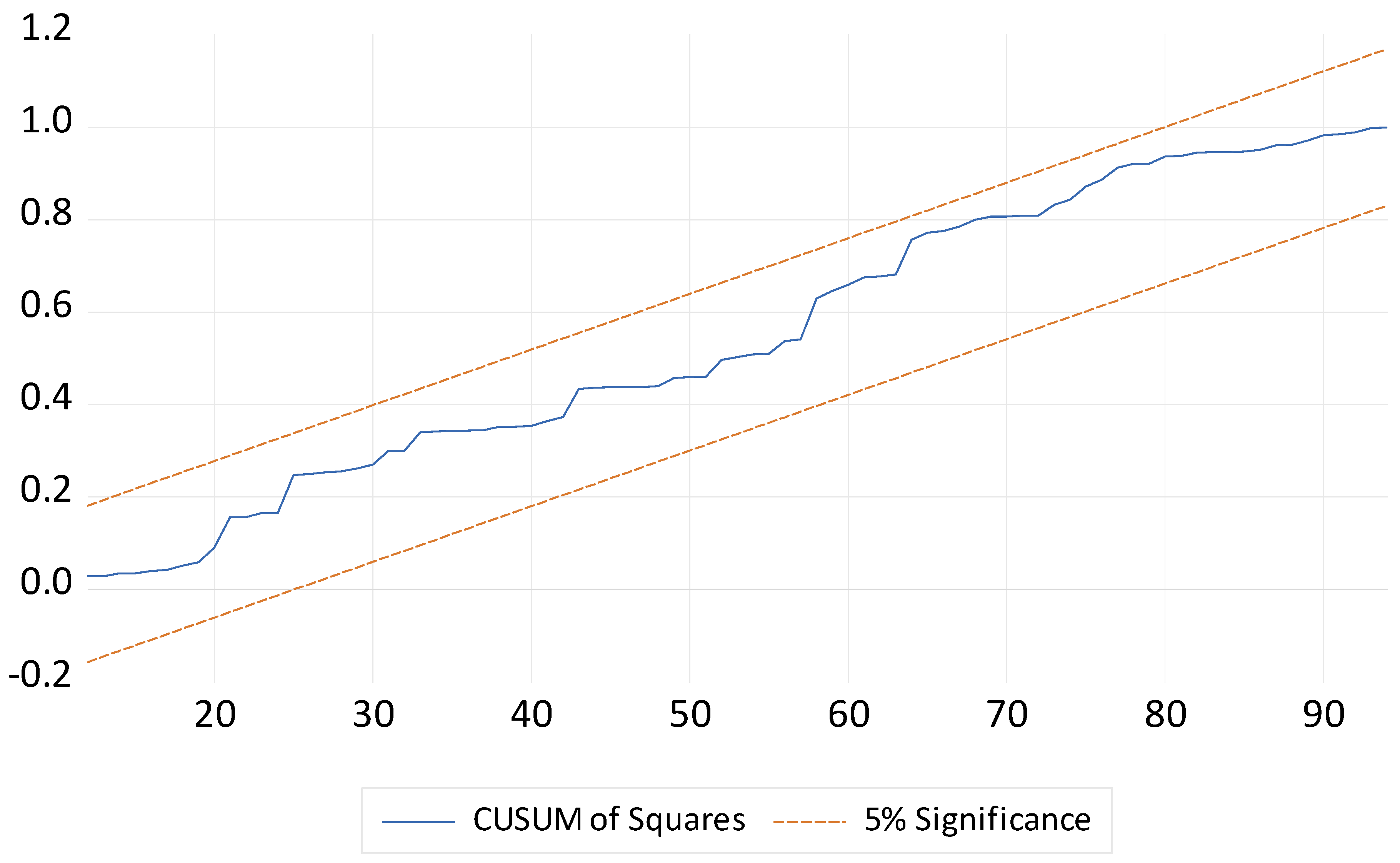
heteroscedasticity	0.6876	0.8184

. The null hypothesis of no serial correlation could not be rejected using the Breusch–Godfrey Serial Correlation LM Test. Also, the null hypothesis of homoscedasticity could not be rejected using the Breusch–Pagan–Godfrey test. Finally, the CUSUM of squares graph shown in Figure 3 confirms the model is dynamically stable.

5. Conclusions

This study offers a methodological improvement in the broader inquiry on the U.S. tourism-growth nexus. It employed the nonlinear autoregressive distributed lag (NARDL) bounds testing approach to confirm cointegration between economic growth and tourism development. Economic growth is measured by real GDP, while tourist arrivals measure tourism development. Two mediating variables, which either stimulate or discourage inbound tourism, were added to the model. These are the exchange rate and implied volatility. While the former is designed to reflect how currency valuation influences the cost-effectiveness of visiting the United States, the latter captures the impact of systematic risk on travel decisions.

As it turns out, the inclusion of the two mediators in the model resulted in cointegration among the variables. More importantly, the findings indicate evidence of long-run bidirectional causality between tourism and growth. Bidirectional causality supports both the growth-led tourism hypothesis and the tourism-led growth hypothesis. The bidirectional effects of growth and tourism are not symmetric, however. Results show that only positive shocks in tourism have a direct causal effect on GDP. On the other hand, only negative shocks in GDP have a causal effect on tourism. Effects of positive shocks to GDP are muted. This study also finds evidence of a one-way short-run causality from GDP to tourism. In the short run, both positive and negative shocks to GDP have a direct although lagged causal effect on tourism. The imputation of causality is in the Granger sense.

The empirical approach in this study differs from existing studies on the tourism-growth nexus in two critical aspects. First, it allows for the inclusion of mediating factors that influence the inbound traveler’s decision. Second, it employs the recently developed asymmetric bounds testing approach to identify and account for important nonlinearities in that relationship. Together, these innovations provide an important path to entangle the asymmetries in the bidirectional relationship between tourism development and economic growth in the case of the U.S.

Unfortunately, data limitation prevents the examination of causal effects that might be attributed to tourism earnings, another important measure of tourism development. The inclusion of this variable in a future study, in addition to market data on tourism stocks, should greatly improve the understanding of the broader economic and financial impact of tourism. Notwithstanding, the findings of this study, similar to those that employ tourist arrivals in their analyses, should offer a substantive insight into the nature and value of inbound tourism in the United States.

6. Economic and Policy Implications

An important implication of this study is the direct impact of the exchange rate on the economic benefit of inbound tourism. Knowing that the decision to visit the U.S. is partly influenced by the purchasing power of the tourist’s home country currency is critical in the marketing of U.S. tourism overseas. There is also the revelation that macroeconomic shocks play a huge part in the travel decision. This sentiment is arguably linked to the country’s preeminence in international geopolitical affairs and perhaps also the high rate of violence in some parts of U.S. Therefore, creating a tourism brand that emphasizes the positives, such as the exchange rate benefits of the U.S. currency and the known vibrancy of many American cities, should prove beneficial.

Importantly, the finding that the exchange rate directly impacts tourism development gives renewed attention to the fourth monetary policy goal of maintaining a stable dollar value. While systematic risks such as international conflicts, economic crises, natural disasters, and pandemics are often unavoidable, there is a need to ensure timely and effective control of their impact. A case can be made about the rather slow response by many countries to the spread of COVID-19 in early 2020. While the severe health risk of this deadly virus was evident by the fall of 2019, many countries, especially those in Europe and North America, were ill-prepared and ill-equipped to deal with the eventual onslaught of this pandemic which came in full force in March 2020. Maintaining adequate preparedness reinforces the need to focus on economic growth and tourism-enabling infrastructure.

Finally, since tourism earnings are a significant portion of U.S. exports, adopting a proactive stance on the tourism sector is critical. This is particularly important because tourism contributes substantially to domestic employment, especially at the low to mid-income levels. Providing timely financial assistance to critical sectors such as hospitality, dining, and entertainment should alleviate the long-term damaging effects of any crisis. There was some demonstration of the U.S. government’s realization of this view when it launched the Paycheck Protection Program (PPP) in spring 2020. This fiscal stimulus was aimed at easing the severe strain of the massive unemployment that came in the wake of COVID lockdowns and quarantines. However, designing such a program in a manner that targets the most vulnerable sectors of the economy should prove even more beneficial. Hospitality, entertainment, and travel-related businesses were the worst affected during the pandemic. Focusing on such businesses recognizes the differential benefit of the travel and tourism industry in providing meaningful jobs to a significant number of service sector employees in the United States.