Article

Old but Resilient Story: Impact of Decentralization on Social Welfare

by
José Luis Alberto Delgado
1,
Dilek Demirbaş
1 and
Ahmet Faruk Aysan
2,*
1
Faculty of Economics, İstanbul University, Beyazıt Kampüs, 34126 Istanbul, Türkiye
2
College of Islamic Studies, Hamad Bin Khalifa University, Doha P.O. Box 34110, Qatar
*
Author to whom correspondence should be addressed.
J. Risk Financial Manag. 2022, 15(12), 584; https://doi.org/10.3390/jrfm15120584
Submission received: 17 October 2022 / Revised: 10 November 2022 / Accepted: 16 November 2022 / Published: 6 December 2022
(This article belongs to the Special Issue Predictive Modeling for Economic and Financial Data)

Abstract

:
This paper analyzes the fiscal performance of Turkey and Argentina during the period 2000–2021, when both countries faced rapid economic growth with the consequent impact on social welfare. This work explored two different systems: Centralization in Turkey and Federalism in Argentina and, in general, studied the decentralization impact of both the systems on social welfare. This study intended to create new social welfare indexes in other regions to analyze the resource allocation in different regions of these countries. As a first step, we built a regional human development index (HDI) for each region. This attempt is considered a new contribution to the literature and intended to fill the gap in this field. Afterward, this index was compared with the fiscal resources allocation (FRA), used as a proxy of fiscal decentralization in an econometric panel data model. By using this method, we concluded that the social welfare indexes have a positive relationship with the fiscal resource allocation in the Federal system, such as in Argentina, but not in the centralized system such as in Turkey during the period analyzed from 2000 to 2020.
JEL Codes:
C43; D6; H3; H11; H21

1. Introduction

The local provision of public goods has led to a series of debates over the last twenty years considered for some the most efficient way to meet public needs in the smaller populations. This debate resulted in the creation of lower levels of government and then the distribution of both, roles and resources to those lower levels of government, which a priori best know the needs of the population. In this way, the responsibility for the provision of public goods lies with sub-central governments and people in these localities have greater power to determine whether governments can better meet their specific needs.
The theory of decentralization is known as Fiscal Federalism, it focuses on the organization of intergovernmental fiscal relations. “Decentralization” generally means the devolution of decision-making powers. A related concept is “decentralization,” in which operations are decentralized, but decision-making powers are not devolved (Martínez-Vázquez 2011; Weingast 1995). It also involves the transfer of responsibility for planning, management, and allocation of resources from the central government and its agencies to field units of government’s agencies, subordinate units, or levels of government (Rondinelli et al. 1986). Oates (1972) developed the theory considering that in the presence of diverse preferences and needs, provision of services from a decentralized government will lead to increased citizen welfare.
In this paper, we compare Turkey and Argentina, two countries, which have both centralized and decentralized features. However, regarding both, the political and fiscal organization and administration, Turkey has a centralized government where the decision-making powers lie at the top level of the government and the public services and goods are provided by all levels. On the other hand, Argentina has a federal organization where the National Constitution assures autonomy to the provinces. Hence both countries provide public services and goods considering the priorities of the local population. In both cases, the funding comes mostly from the central government because this level has the power to collect the most important taxes in the country—income and consumption—so decisions regarding bigger resource allocation such as road projects, for example, are taken at the central level (Tiebout 1956).
We have chosen Turkey and Argentina, because, in addition to the characteristics mentioned above, they experienced sustained economic growth between 2002 and mid-2010s; both countries have similar economic and productive structures. Moreover, both have experimented with the similar political and economic processes and crisis, during this period and in the past (Aysan et al. 2013a, 2016).
The Theory of Fiscal Decentralization studies all levels of government cooperation for efficient resource allocation. The ideal system would be a centralized one with perfect information about the demands of the whole population so it can take the right decision to protect them from the shocks, preserving the power to modify allocations without any kind of bureaucratic process, which is impossible. Given the political process’ natural constraints, we want to measure up to which level the institutions in each country allocate resources according to the evolution of the minimum standard life indexes (Tanzi 2000).
To have a standard comparison, we choose the human development index as a proxy for a group of several basic variables. This index is made by the United Nations (UN) to put in one single number of three key life standard variables: “literacy”, related to education; “life expectancy”, related to health and “income”, related to purchasing power and consumption capacity. Unfortunately, this index is published at a national level, and, as we should consider the locals and regional levels we need to adapt this index to lower population levels.
The most important contribution of this paper is to develop a new Regional Human Development Index (RHDI from now on). Hence we managed to compare it with the fiscal Resources Allocation (FRA) for every region of both countries. In order to build our index, we took the information from several official institutions, such as TürkStat and The Ministry of Finance in Turkey and INDEC, the National Institute of Statistics, and the Ministry of Economics, in Argentina. With this research, as we want to find if given the institutional framework, there is any relation between the allocation and the demand from the population in both countries and if and how the government adopts it dynamically in both countries, we analyzed through a data panel model the impact of our RHDI that we made following the methodology used by the United Nations on fiscal income and spending decentralization for each region between 2002 and 2021. We divide Argentina into 5 regions and Turkey into 16 regions according to the division made by its own National Statistics institutes (Sağbaş et al. 2003; Gonzalez et al. 2014).
By comparing both systems, the key result of this paper is that the Federal systems can understand better the locals’ needs and fix the market failures. By analyzing the case of the Argentinean, the joint work between the central government and local government in the federal system can moderate market failures and reduce inequalities so individuals and firms can participate in the benefits of a competitive economy.
We start our research by reviewing the literature related to welfare economics and fiscal decentralization in Section 2. In Section 3, we explained our methodology to analyze the relationship between resources allocation and Human Development Index and we run our models for each country in Section 3. Finally, Section 4 presents the conclusion, reference, and data annexed.

2. From Welfare Economics to Decentralization Policies

Decentralization as economic research field started in early fifties when Paul Samuelson (1954) showed that in the case of private goods market system can respond accurately to the preferences of each, but on the other hand, the provision of public goods responds to aggregate preferences, no one receives according to their individual preferences, which is a problem of efficiency.
Years later Ostrom et al. (1961), analyzed the case of the provision of public services in a big city. They discovered that it would be more efficient than decentralized users in each district to face the local costs because this way there would be a better match with the preferences of citizens, as long as such provision can be circumscribed territorially and there are no economies of scale to justify a centralized provision.
Indeed, from the analysis of Samuelson, it seems clear to the extent that different levels of subnational communities can autonomously take decisions, they are closer to their respective distinct collective preferences and individual preferences. Studies on measuring welfare related to fiscal decentralization (FD) policies are not new; however, as the developing economies grew at different levels during the last 30 years, the way of theorizing and measuring those impacts had been changing to find the appropriate way to study how the institutional framework and policymakers adapt to new realities (Besley 2002).
In this line, Martínez-Vázquez et al. (2017) studied what they considered unsolved issues in the empirical literature on decentralization: the proper measurement of decentralization itself and its potential endogeneity in econometric estimates. Following this line, Neyaptı (2005), Aslim and Neyaptı (2017) presented a study to analyze the welfare and redistributive effects of FD. They found that as an increase in the tax rate reduces tax effort, fiscal decentralization increases to improve welfare. They showed that extreme levels of FD lower welfare and worsen income distribution. When regional spillovers exist, increasing FD decreases welfare and redistribution (Aysan et al. 2013b).
Badrudin (2013) made a similar empirical study but focused on six cities in Central Java Province, Indonesia. Their results showed that fiscal decentralization has a significant effect on economic growth and social welfare; capital expenditure has no significant effect on economic growth and social welfare, and economic growth has a significant effect on social welfare. On the other hand, and considering the dynamic context, Rodden and Wibbels (2010) studied the cyclicality of budget items among provincial governments in seven federations, showing that own-source taxes are generally highly pro-cyclical, and contrary to common wisdom, revenue sharing and discretionary transfers are either acyclical or procyclical. The resulting procyclicality of provincial fiscal policy is likely to have important implications in a world where demands for countercyclical fiscal policy are increasing but considerable fiscal responsibilities are being devolved to subnational governments.
As we can see in the previous literature, there are studies that show the efficiency in the allocation of resources and its distributive effects of the fiscal decentralization policy, as well as the dynamic adaptation of the budget and the welfare effects; however, we also find that having an adequate measure of the allocation of resources given different measures of well-being are partially adequate since they do not contemplate in most cases the contemporary measures of human development. By not taking into account these international standards, the local needs and the institutional framework are not connected. In this work we are trying to understand if this political intervention leads to a more competitive economy, looking for Pareto efficiency. A competitive market should increase the production possibilities frontier and finally, achieving to human better development.

3. Methodology

The current research aims to study how the degree of decentralization affects the allocation of resources according to the evolution of the welfare of population in regional levels. That is, we suppose the government look at the social and welfare variables evolution and relocate the resources dynamically. To analyze welfare, we use one unique variable that describe general welfare in the most approximate possible way. Hence, we choose the human development index as a proxy of a group of several basic variables. This index is made by the United Nations (UN) to put in one single number three key life standard variables: literacy, related to education; life expectancy, related to health; and income, related to buy power and consumption capacity. To do it so, we adapt UN methodology to lower population levels, and we build our Regional Human Development Index (RHDI), so we can compare with the income allocation for every region of both countries. Finally, we analyze the relationship between fiscal decentralization; this is the amount of funds sent to every region and the HDI in each region using a data panel.
This method provided a power of analysis of the situation government faces and how they decide to use the resources in order to fix market failures.
The data we use in this research are from Türk Istatistik Kurumu (TÜİK), which is the National Statistics Institution in Turkey; The National Fiscal Coordination Office (DNCFP—Dirección Nacional de Coordinación fiscal con las Provincias) and Statistics National Institute (INDEC—Instituto Nacional de Estadísticas y Censos) in Argentina. Both data are in local currency, so we change to U.S. Dollars at the exchange rate of the referred time. As a first step, we separate each country in geographical regions. Table 1 and Table 2 show both the Turkish regions and the Argentinian regions.

3.1. Description and Variables Estimation

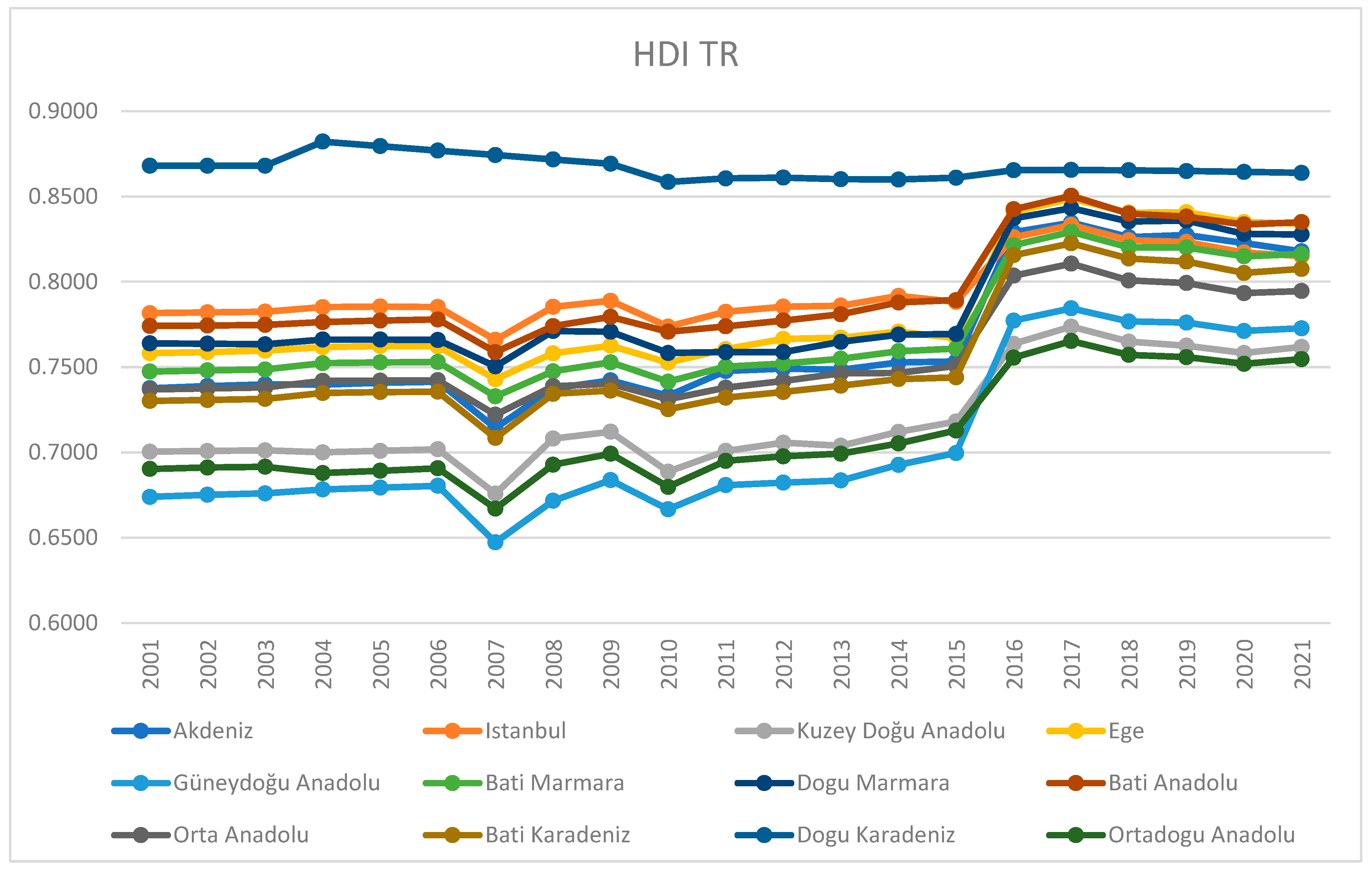
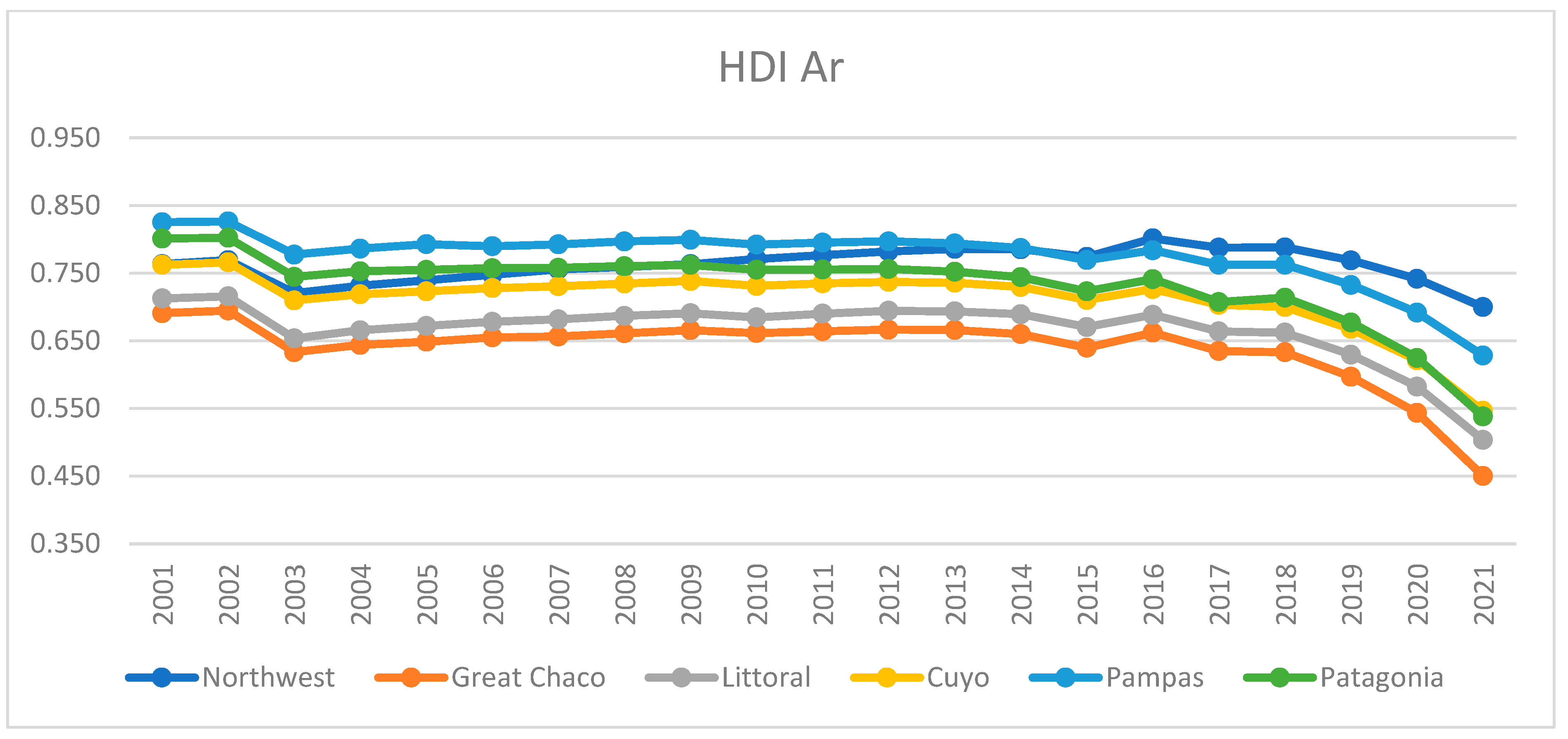
3.1.1. Human Development Index (HDI) Construction

The second part includes the estimation of our HDI for each region, which we obtain as an average of all provinces in each region. Hence, we use the same methodology to construct the index at national level. That is to say, we use the same variables as “years of education”; “life expectancy”; “Income per capita” for every province and every region. Then, to estimate the index we use the following formulas:
  • Life Expectancy Index (LEI):
    L E I = L E 20 85 20
    where LE is the life regional life expectancy
  • Education Index (EI):
    E I = M Y S I + E Y S I 2
    where MYSI is mean years of School Index: MYSI = M Y S 15 ; and EYSI is expected years of schooling index: EYSI =
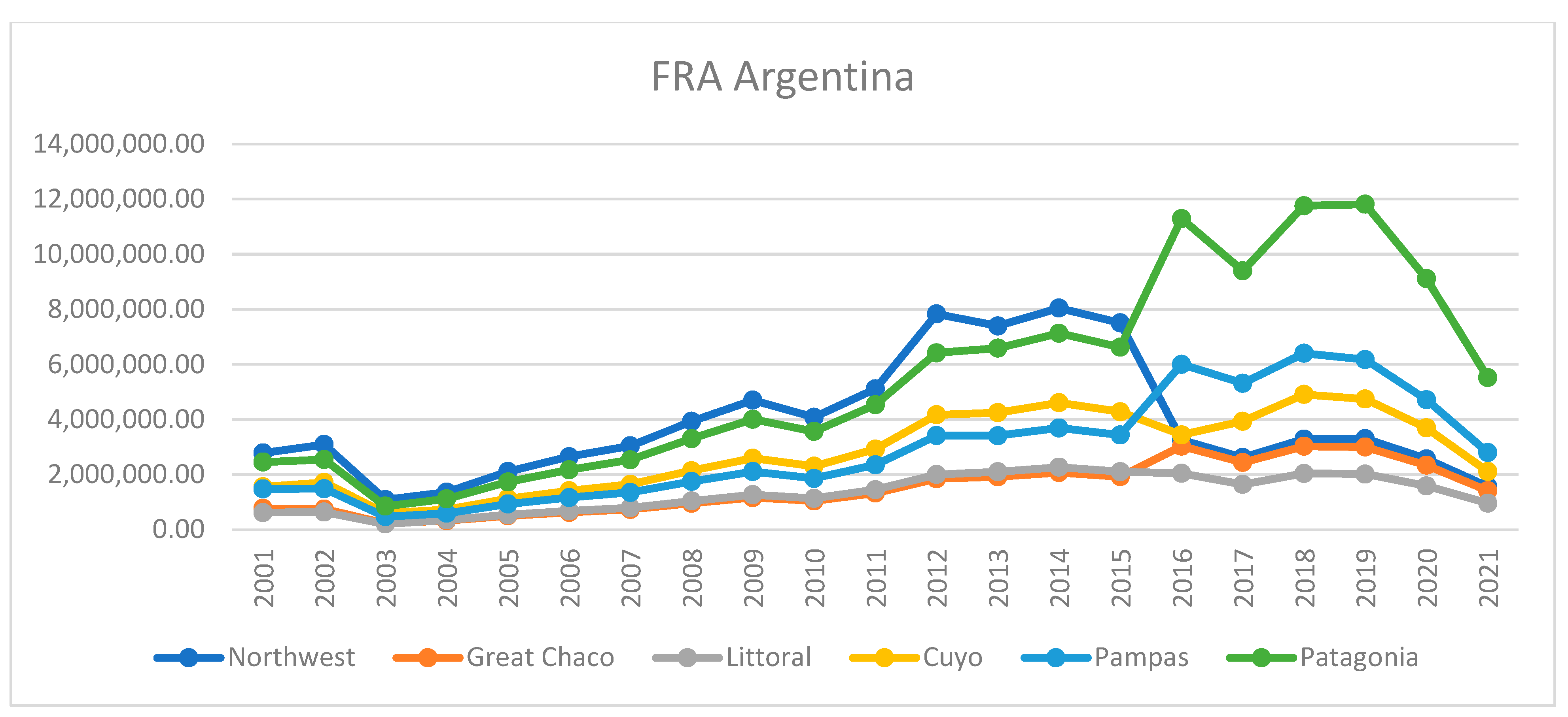
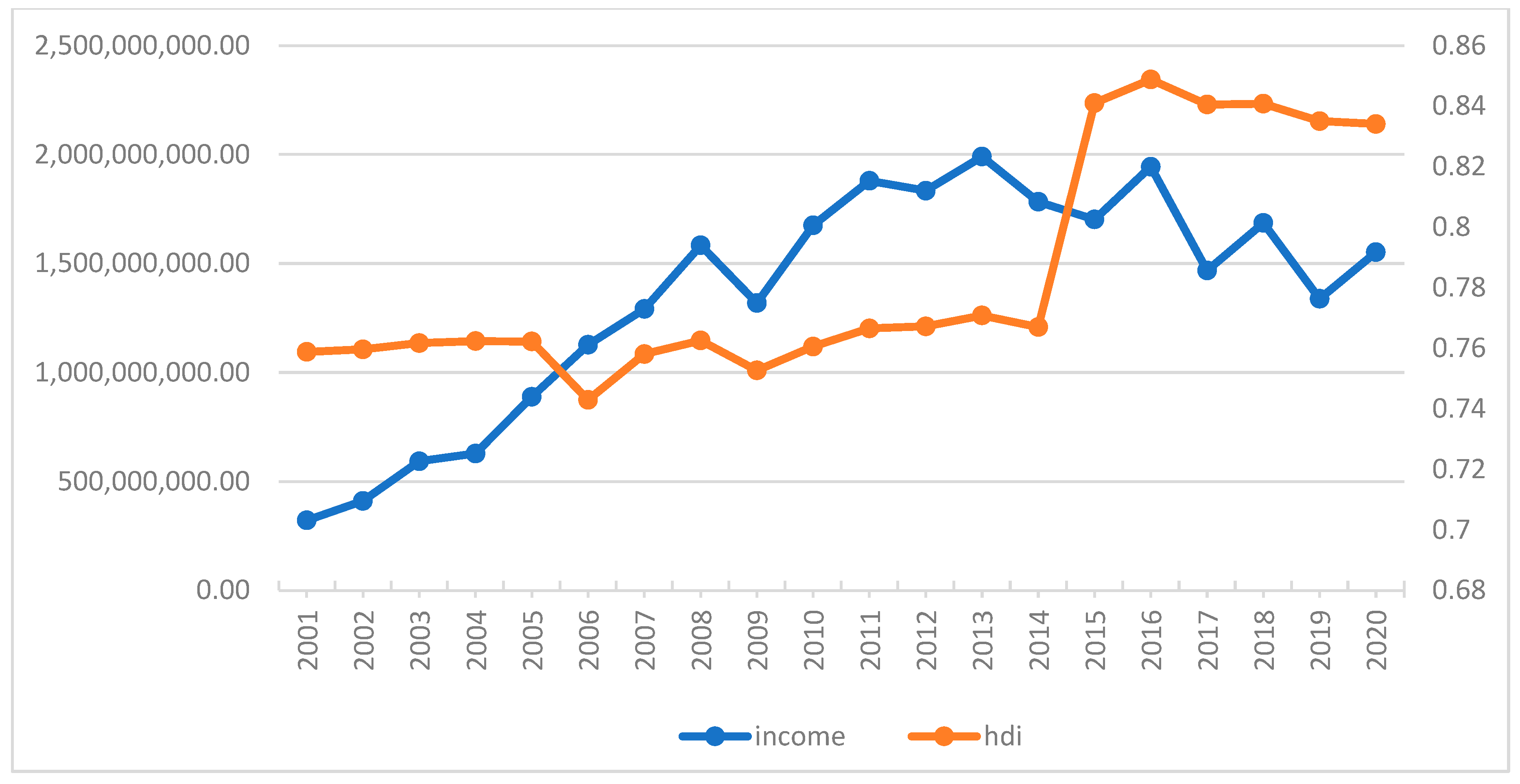
 E Y S 18
  • Income Index (II):
    I I = ln ( G N I p c ) ln ( 100 ) ln ( 75000 ) ln ( 100 )
    where GNIpc is the regional gross domestic Income per capita.
  • Finally, the human development index we obtain as follows:
    H D I i t = L E I i t × E I i t × I I i t 3
    where HDIit is the human development index for the region “i” for the year “t”. In this index the outcome can be a number between 0 and 1, where 0 is worst situation and 1 is the best situation.

3.1.2. Data Description

Once we obtain the HDIs, we compare its possible correlation with fiscal resources allocation (FRA) for each region. For example, in the following charts we can see the evolution of both HDI and FRA for “Istanbul”; “Ege” and “Güneydoğu Anadolu”, in the case of Turkey; and “Pampas”, “Gran Chaco” “Cuyo” in the case of Argentina. In all of them, the slope of the points shows a growth trend. Consequently, over the years, and with the FRA increase we see an increasing regional HDI.
During the period under review (2001–2021) as shown in Figure 1, the HDI estimations for Turkey are around 0.6473 (Güney Doğu Anadolu) in 2006 and 0.8821 (Doğu Karadeniz) in 2003. The highest HDI is in Doğu Karadeniz, Ege and Istanbul, and in some cases is above the national estimation. For example, in 2013, the United Nations Development Program (UNDP) estimated a national HDI of 0.7591, in that year we estimate 0.792 for Istanbul, 0.771 for Ege, and 0.86 for Doğu Karadeniz. As can be seen from Figure 1, whilst the lowest HDI in Turkey is for Güneydoğu Anadolu, the highest HDI is for İstanbul. In annexed, HDI for Turkey on a yearly basis is shown in followed tables.
When we look at Argentina case, whilst the lowest HDI in Argentina generates for Great Chaco, the lowest HDI generates for Pampas till 2016 and then for northwest regions in Argentina as can be seen from Figure 2. In annexed, HDI for Argentina on a yearly basis is also shown in followed tables.
In the Figure 1 and Figure 2, we can see the evolution of the HDI for both series, where we included since 2000 to assess the impact of the 2002 devaluation in the case of Argentina. At the same time, we found a HDI under the national estimation for Kuzey Doğu Anadolu, Güney Doğu Anadolu, Bati Karadeniz where we estimate 0.712, 0.693, and 0.743, respectively.
Meanwhile, in the case of Argentina, our data was estimated from 0.633 for the region of Gran Chaco in 2002. We must consider that during this year Argentina suffered a severe devaluation after they left the currency peg system that abruptly struck the income and purchasing power of the people, especially the country’s poorest regions. Meanwhile, the highest rate is estimated at 0.799 for 2008 in the Pampas region, which is the richest in the country and maintains the highest regional HDI estimated for the entire period.

3.2. Panel Data Analysis

An econometric panel data model includes a sample of agents for a given period. So, the essential feature of panel data is available for both temporal and spatial dimensions. As an example, you can have annual data on income, HDI, income per capita, among others, in 12 regions in Turkey or 6 regions in Argentina for a period of 13 years (2002–2014), which is a base of mixed data time series and cross-section, becoming panel data. In this example, the sample elements are time and the regions.
The main objective of implementing and studying the data panel, is to capture the unobservable heterogeneity, either between agents as well as in time, given that this heterogeneity cannot be detected nor time series studies nor with cross section (Baronio and Vianco 2012).
This technique allows for a more dynamic analysis by incorporating temporal dimension of the data analysis, which enriches the study. While working with this kind of information as part of unobserved heterogeneity, the application of this methodology allows analyzing two aspects of importance:
(i)
The specific, individual effects and;
(ii)
Temporary effects.
The individual effects are those that affect unevenly each study agents contained in the sample which are time—invariant and directly affect the decisions made by these units, such effects are usually identified with issues of entrepreneurship, operational efficiency, experience capitalization, access to technology, etc. On the other hand, the temporary effects are those which apply equally to all individual units of study. Such effects may be associated, for example, to macroeconomic shocks that can affect equally to all companies and units of study.
The first specification refers to the case where there is no heterogeneity observable in the data system panel and therefore the ordinary least squares method with the advantage of winning degrees of freedom is used. However, in cases where the homogeneity hypothesis is rejected in a system panel data, so there is heterogeneity observable either over time between study either units (individuals) or in both directions; there must be sought a specification that capture properly to avoid the problem of bias on estimates of the parameters of the explanatory variables, which would be committed if the specification is used.
There are two additional procedures to estimate the model in a data system panel: one involves the recognition that omitted variables may lead to changes in the intercepts either over time or between cross-sectional units, in this case the fixed effects model attempts to approximate these changes with dummy variables; The other model is the random effects, which tries to capture these differences through the random component of the model.
As already mentioned, the technique of panel data allows us to contemplate the existence of specific to each unit of cross-sectional individual effects, time invariant that affects how each unit cross section makes its decisions. A simple way, and, in fact, the most widely used, considering this heterogeneity is using variable intercept models. Thus, the linear model is the same for all units or individuals under study, other is the also done for robustness and the results are same.
This model assumes that there is a different constant term for every individual and assumes that the individual effects are independent of each other. With this model it is considered that the explanatory variables affect both the cross-sectional units and they differ in characteristics of each, measured by the intercept features. Therefore, the n intercepts are associated with dummy variables with specific coefficients for each unit, which must be estimated. Then, we can write the model as follows:
Y i t = α i t + β 1   X 1 i t + β 2 X 2 i t + + β k X k i t + U i t
  • i = 1, 2, 3, …, n
  • t = 1, 2, 3, …, T
For start our work, we present the data in a table attached to both Argentina and Turkey. In the case of Argentina, we have 132 observations, while for Turkey, 156 cases. There are 20 years covered (observations) for each region in both countries.
We intend to analyze the impact of population welfare, measured by the regional HDI (X) in amount of fiscal resources allocation (Y) that we use as a proxy for fiscal decentralization, but use the HDI of the previous year, so we can see if the authority reacts to a certain level of welfare and take a decision regarding to the allocation in a similar model presented by Martínez and Aldo (2009). Finally, the standard model is presented as follows:
l n F R A i t = β 1 + β 2 L n H D I 1 i t + μ i t
By having a panel where all data are complete for each of the periods, the panel data used in the regressions (6) is hence balanced. Where “LN_FRA” is the logarithm of the fiscal Resources allocation amounts of money in U.S. Dollars from central government to the “i” in the “t” year. On the other side, we have “LnHDI” which is the estimated logarithm of the human development index for the “I” region in the year “t − 1”.
Before running the econometric estimations, we must determine which model we should apply: either random effects or fixed effects model. The fixed effect or LSDV model allows for heterogeneity or individuality among the regions by allowing having its own intercept value. The term fixed effect is due to the fact that although the intercept may differ across regions, but intercept does not vary over time, that is it is time invariant. In the random effect model, we have to find a common mean value for the intercept across the regions. So, to determine the model we run Hausman Test for the following hypothesis;
H0. 
Random effects model is appropriate.
H1. 
Fixed effects model is appropriate.
If we find a statistically significant p-value, we should use fixed effect model, otherwise, the random effect model. So, after running the Hausman Test model for the case of Turkey in Table 3, we found that random effect model is the appropriate one.
We can see that the p-value is bigger than the accepted thresholds in the literature. Hence, we cannot reject the null hypothesis. Then, the best model for estimation is the random effects model.
In the same direction, we test for Argentina and the outcome is as follows in Table 4:
Nevertheless, for the Argentinian case, the p-value is very small, so we reject the null hypothesis, and we conclude that the most appropriated model is the fixed-effects one.
The outcome model for Argentina is in Table 5 and Table 6:
From the first analysis we can see that the constant is negative. This is an intuitive outcome because of the Argentinian Partnership Act that forces the central government to send money to local levels without any kind of reference or parameter. Moreover, there is positive relationship of the coefficient of “ln_hdi_ar” (intuitive and expected result), and with 95% confidence it has individual statistical significance (t = 2.32), which means that the regional standard welfare index has individual effect on the allocation from central government. We can conclude that, instead of our incomplete model because of a low R-square and DW statistic, the regional HDI from one year before is considered when the central government has to allocate resources to lower government levels.
Finally, the outcome model for Argentina is:
L O G   ( F R A ) = 2216623 + 7332137   L O G   ( R H D I ) t 1 1287469 d 1 2088449 d 2 2051708.4 d 3 190414.09 d 4 + 420119.59 d 5 + 2622982 d 6
(di = 1 for observations of region i and di = 0 in a different case).
The regression results for the case of Turkey are given in Table 7 and Table 8:
From the previous estimation for the case in Turkey, we found a negative and non-statistical significance for the variable “LN_HDI_tr” in the fiscal resources allocation from the central government. So, according to our estimation the regional welfare indexes evolution is not considered by the government to change the resources allocation during the analyzed period.
On the other hand, we have the data of tax revenue collected by the provinces and hence for the corresponding regions for the variable FRA for both countries in Figure 3 and Figure 4. After the economic crisis and the devaluation suffered in Argentina, a sharp drop is seen in the income received by the regions.
Finally, the outcome model for Turkey is:
L o g   ( F R A ) = 3350000 2640000   L o g   ( R H D I ) t 1 1200000 d 1 1562000 d 2 8851000 d 3 1325000 d 4 7533000 d 5 1201000 d 6 1269000 d 7 1544000 d 8 + 1269000 d 9 2162000 d 10 7864000 d 11
Figure 3 shows the fiscal resource allocation from central government to regions in Turkey from 2000 to 2021. While İstanbul gets the highest share, Doğu Karadeniz and Ortadoğu Anadolu regions get the lowest share from the central government. Nevertheless, even for İstanbul the share gradually declines after 2016 as a result of high devaluation. In annexed, FRI for Argentina on a yearly basis is also shown in Table 9, Table 10, Table 11 and Table 12; and HDI for Turkey on a yearly basis is also shown in Table 13, Table 14, Table 15 and Table 16.
Similarly Figure 4 shows the fiscal resource allocation share from central government to regions in Argentina from 2000 to 2021. While Patagonia region gets the highest share, Uttoral region gets the lowest share from the central government. However, after 2016, even for Pattogonia the share from central government starts to decline because of devaluation.
When we combine these two variables RHDI and FRA, then we can see the trend of these two variables and work on the data from 2000 to 2021 in Figure 5, Figure 6, Figure 7, Figure 8, Figure 9 and Figure 10.
In addition, the latest data published by UNDP for the whole country, also refers to the year 2013 and estimates an HDI of 0.808. For this year, no region reaches that value; only the northwest region reaches a value of 0.785 and Pampas region worth 0.787. Meanwhile, the “Gran Chaco” again recorded in lower data with just 0.66.

4. Conclusions

We began our research wondering whether the resources allocated to lower levels of government have relationship with basic general needs. If fiscal decentralization is a function of the minimum demands of the population is later summarized in an indicator measuring welfare in our model by the regional human development index (HDI).
Regarding only to fiscal decentralization both in Turkey and in Argentina, we described two different political systems and consequently two different tax and allocation systems. On one side is Turkey with a unitarian system where political and power decisions are taken from the central government level and decentralize only the provision of certain services of provincial or municipal characteristics. We found that in the case of Turkey the central government decides each year, which services the provinces and/or municipalities provide and how much money should be transferred to it. This system could be more dynamic, since the central government can take money from one province and put to another without any legal restriction or any kind of bureaucratic delay, in example, sending bills to National Parliament. However, it can also be quite unpredictable and subject to the political link between the central government and the local one; but these issues go further than the analysis we want to do in this research. On the other hand, Argentina has a federal system of government, annually allocates a portion of its main revenue (taxes on income and consumption) directly to the provinces and complemented by specific transfers. Only the latter portion is dynamic and can be adaptive for current needs, political agreements, and so on. Hence, the Argentinian provinces decide with the money they receive what benefits should pay in each of their respective jurisdictions and have an income profile of long-term more predictable, allowing better planning at the local level. Another feature is that voters can elect people they believe will best meet their needs or, fix the market failures locally.
As mentioned in the introduction of work, we do not seek to analyze which system is better or more effective. But through the comparison of these two countries with similar economic structures, as well as similar processes of crisis in recent years, but different systems of decentralization we can have a first approximation of which one of them has built a system that responds in a better way to the social welfare indexes even if the political system is unitarian or federal. So, to answer these questions we made a regional human development index for every region inside each country from 2001 to 2020 as a proxy of social welfare index and we analyzed if there was any kind of relationship with the resources allocation, that we used as a proxy of fiscal decentralization.
We used a regional HDI because inside this index we can include both economics and welfare variables. Since the methodology for building the index includes “literacy”, “life expectancy”, and “local gross domestic product (GDP)”; this index resumes in only one number between 0 and 1 (0 as worst situation and 1 is the best situation) how good are the standard life and opportunities in one region inside both countries.
In the case of Turkey, we found a positive relationship, as expected, between fiscal decentralization and regional human development index, but no statistical significance. Finally, our model cannot totally explain whether the unitarian system in Turkey allocates or not funds according to welfare indexes during the years we analyzed. In the case of Argentina, the results are also not fully explanatory. At this point we must remark that if the study considers until only 2016, the results suffered several changes. However, after this year, both countries again suffered devaluation processes that affected severely the income and welfare. Finally, the model should use additional variables to reach to appropriate understanding of the fiscal distribution in both countries.
As final comments, we can say that in the Argentinian case, the joint work between the central government and local government in the federal system can moderate market failures and reduce inequalities so individuals and firms can participate in the benefits of competitive economy. On the other hand, in the case of Turkey, during the analyzed period the joint work between the different levels of government cannot assure equal opportunities so the markets failures may exclude agents from the benefits of more competitive economy.

Author Contributions

J.L.A.D.: Conceptualization, methodology, investigation, software, writing—original draft preparation. D.D., A.F.A.: validation, formal analysis, resources, data curation, writing—review and editing, supervision. All authors have read and agreed to the published version of the manuscript.

Funding

This research activity/output was supported under the HBKU CIS’ Research Clusters Grant.

Institutional Review Board Statement

Not applicable.

Informed Consent Statement

Not applicable.

Data Availability Statement

Not applicable.

Conflicts of Interest

The authors declare no conflict of interest.

Note

1
Source: https://www.undp.org/turkiye/ (accessed on 2 September 2022).

References

  1. Aslim, Erkmen Giray, and Bilin Neyaptı. 2017. Optimal fiscal decentralization: Redistribution and welfare implications. Economic Modelling 61: 224–34. [Google Scholar] [CrossRef] [Green Version]
  2. Aysan, Ahmet Faruk, Huseyin Ozturk, Ali Yavuz Polat, and Burak Saltoğlu. 2016. Macroeconomic Drivers of Loan Quality in Turkey. Emerging Markets Finance and Trade 52: 98–109. [Google Scholar] [CrossRef]
  3. Aysan, Ahmet Faruk, Mustafa Disli, and Koen Schoors. 2013a. Bank Competition and Outreach: Evidence from Turkey. Emerging Markets Finance and Trade 49: 7–30. [Google Scholar] [CrossRef] [Green Version]
  4. Aysan, Ahmet Faruk, Mustafa Haluk Güler, and Cüneyt Orman. 2013b. Sustaining Growth in Emerging Markets: The Role of Structural and Monetary Policies. In A New Model for Balanced Growth and Convergence. Cheltenham: Edward Elgar Publishing, pp. 122–44. [Google Scholar]
  5. Badrudin, Rudy. 2013. Effect of Fıscal Decentralızatıon On Capıtal Expendıture, Growth, And Welfare. Economic Journal of Emerging Markets 3: 211–23. [Google Scholar] [CrossRef]
  6. Baronio, Alfredo, and Ana Vianco. 2012. Datos de Panel Guía para el uso de Eviews. Córdoba: Departamento de Matemática y Estadística, Facultad de Ciencias Económicas, Universidad Nacional de Río Cuarto. Available online: http://www.econometricos.com.ar/wp-content/uploads/2012/11/datos-de-panel.pdf (accessed on 1 March 2015).
  7. Besley, Timothy. 2002. Welfare Economics and Public Choice. London School of Economics and Political Science. Available online: http://www.lse.ac.uk/economics/people/facultyPersonalPages/facultyFiles/TimBesley/WelfareEconomicsandPublicChoice.pdf (accessed on 25 January 2016).
  8. González, Lucas, Marcelo Gabriel Nazareno, Sergio Víctor Barone, Sebastián Freille, Santiango Alles, and Julieta Lenarduzzi. 2014. Impacto Regional de los procesos de decentralización fiscal: Desarrollo y equidad en América Latina. Fundación Carolina. Serie Avances de Investigación 68; Madrid: Fundación Carolina. Available online: http://www.fundacioncarolina.es/wp-content/uploads/2014/08/AI68.pdf (accessed on 1 March 2015).
  9. Martínez, André, and Musacchio Aldo. 2009. Dotación de Factores, Federalismo Fiscal y el Costo de Capital de los Estados: Evidencia para Brasil, 1891–1930. Banco de México. Available online: http://www.banxico.org.mx/publicaciones-y-discursos/publicaciones/documentos-de-investigacion/banxico/%7B9F4891DD-E89F-E673-717C-895A5FF83363%7D.pdf (accessed on 10 April 2016).
  10. Martínez-Vázquez, Jorge. 2011. The Impact of Fiscal Decentralization. Issues in Theory and Challenges in Practice. Mandaluyong: Assian Development Bank. Available online: http://www.adb.org/sites/default/files/publication/28927/impact-fiscal-decentralization.pdf (accessed on 1 March 2015).
  11. Martínez-Vázquez, Jorge, Santiago Lago-Peñas, and Agnese Sacchi. 2017. The Impact of Fıscal Decentralızatıon: A Survey. Journal of Economic Surveys 31: 1095–129. [Google Scholar] [CrossRef] [Green Version]
  12. Neyaptı, Bilin. 2005. Equalization via Fiscal Decentralization. Ankara: Turkish Economic Association, Bilkent University. Available online: http://www.tek.org.tr/dosyalar/Bilin-2.pdf (accessed on 10 January 2016).
  13. Oates, Wallace. 1972. Fiscal Federalism. New York: Harcourt Brace Jovanovich. [Google Scholar]
  14. Ostrom, Vincent, Charles M. Tiebout, and Robert Warren. 1961. The Organization of Government in Metropolitan Areas: A Theoretical Inquiry. The American Political Science Review 55: 831–42. [Google Scholar] [CrossRef]
  15. Rodden, Jonathan, and Erik Wibbels. 2010. Fıscal Decentralızatıon and the Busıness Cycle: An Empırıcal Study Of Seven Federatıons. Economics & Politics 22: 37–67. [Google Scholar] [CrossRef]
  16. Rondinelli, Dennis A., James S. McCullough, and Ronald W. Johnson. 1986. Analysing Decentralization Policies in Developing Countries: A Political-Economy Framework. Available online: http://dess.fmp.ueh.edu.ht/pdf/colloque2012_Rondinelli_analyse_decentralisation_economie_politique.pdf (accessed on 2 March 2015).
  17. Sagbas, Isa, Huseyin Sen, and Muhsin Kar. 2003. Fiscal Decentralisation, The size of Public sector and Economic Growth in Turkey. Available online: http://www.diw-berlin.de/documents/dokumentenarchiv/17/41395/Paper-160.pdf (accessed on 2 March 2015).
  18. Samuelson, Paul. 1954. The Pure Theory of Public Expenditure. The Review of Economics and Statistics 36: 387–89. [Google Scholar] [CrossRef]
  19. Tanzi, Vito. 2000. On Fiscal Federalism: Issues to Worry About. Tokyo: IMF. Available online: https://www.imf.org/external/pubs/ft/seminar/2000/fiscal/tanzi.pdf (accessed on 1 March 2014).
  20. Tiebout, Charles M. 1956. A Pure Theory of Local Expenditures. Journal of Political Economy 64: 416–24. Available online: http://www.unc.edu/~fbaum/teaching/PLSC541_Fall08/tiebout_1956.pdf (accessed on 2 March 2015). [CrossRef]
  21. Weingast, Barry. 1995. The Economic Role of Political Institutions: Market-Preserving Federalism and Economic Development. Journal of Law, Economics and Organization, 1–31. Available online: https://web.stanford.edu/group/mcnollgast/cgi-bin/wordpress/ (accessed on 1 March 2015).
Figure 1. HDI Turkey evolution. Source: Turk Statistical Institute.
Jrfm 15 00584 g001
Figure 2. HDI evolution Argentina. Source: United Nations.
Jrfm 15 00584 g002
Figure 3. FRA Turkey (USD). Source: Turk Statistical Institute.
Jrfm 15 00584 g003
Figure 4. FRA Argentina (USD). Source: DNCFP.
Jrfm 15 00584 g004
Figure 5. RHDI and FRA Istanbul 2001–2021. Source: Turk Statistical Institute.
Jrfm 15 00584 g005
Figure 6. RHDI and FRA Ege 2000–2021. Source: Turk Statistical Institute.
Jrfm 15 00584 g006
Figure 7. HDI and FRA Güneydoğu Anadolu 2001–2021. Source: Turk Statistical Institute.
Jrfm 15 00584 g007
Figure 8. HDI and FRA Pampas 2000–2014. Source: DNCFP.
Jrfm 15 00584 g008
Figure 9. HDI and FRA Great Chaco 2001–2021. Source: DNCFP.
Jrfm 15 00584 g009
Figure 10. HDI and FRA Cuyo 2001–2021. Source: DNCFP.
Jrfm 15 00584 g010
Table 1. Regions and Provinces of Turkey.
RegionsProvinces
AkdenizAdana, Antalya, Burdur, Hatay, Isparta, Mersın, Kahramanmaraş, Osmaniye
Istanbulİstanbul
EgeAfyonkarahisar, Aydın, Denizli, İzmir, Kütahya, Manisa, Muğla, Uşak
Güney Doğu AnadoluAdıyaman, Diyarbakır, Gaziantep, Mardin, Siirt, Şanlıurfa, Batman, Şırnak, Kilis
Batı MarmaraBalıkesir, Çanakkale, Edirne, Kırklareli, Tekirdağ
Doğu MarmaraBilecik, Bolu, Bursa, Eskişehir, Kocaeli, Sakarya, Yalova, Düzce
Batı AnadoluAnkara, Konya, Karaman
Orta AnadoluKayseri, Kırşehir, Nevşehir, Niğde, Sivas, Yozgat, Aksaray, Kırıkkale
Batı KaradenizAmasya, Çankırı, Çorum, Kastamonu, Samsun, Sinop, Tokat, Zonguldak, Bartın, Karabük
Doğu KaradenizArtvin, Giresun, Gümüşhane, Ordu, Rize, Trabzon
Orta Doğu AnadoluBingöl, Bitlis, Elazığ, Hakkari, Malatya, Muş, Tunceli, Van
Kuzey Doğu AnadoluAğrı, Erzincan, Erzurum, Kars, Bayburt, Ardahan, Iğdır
Source: Türk Stat.
Table 2. Argentinian Regions.
RegionsProvinces
NoroesteCatamarca, Jujuy, Salta, Tucumán
Gran ChacoChaco, Formosa, Santiago del Estero
LitoralCorrientes, Entre Ríos, Misiones
CuyoLa Rioja, Mendoza, San Juan, San Luis
PampaBuenos Aires, Cordoba, La Pampa, Santa Fé, Ciudad Autónoma de Buenos Aires
PatagoniaChubut, Neuquén, Río Negro, Santa Cruz, Tierra del Fuego
Source: INDEC.
Table 3. Hausman Test Turkey.
VariableFixedRandomStd Dev (Diff)Prob.
Ln_hdi_tr18.59 × 10+108.36 × 10+104.54 × 10+100.6103
Table 4. Hausman Test Argentina.
VariableFixedRandomStd Dev (Diff)Prob.
Ln_hdi_ar1−8,128,830−5,168,6791,031,2260.0041
Table 5. Estimation for Argentina.
VariableCoefficientStd. Errort-StatisticProb.
LN_HDI_AR17,332,1373,155,2042.320.022
C−2,216,6232,264,895−0.980.330
R2 = 0.0417, F-statistic = 5.40.
Table 6. Cross-section effects for Argentinians Regions.
Cross-Section Effects
Northwest−1,287,469.9
Great Chaco−2,088,449
Litoral−2,051,708.4
Cuyo−190,414.09
Pampas420,119.59
Patagonia2,622,982
Table 7. Estimation for Turkey.
VariableCoefficientStd. Errort-StatisticProb.
LN_HDI_TR1−2.64 × 10+105.32 × 10+10−0.500.620
C3.35 × 10+104.08 × 10+100.82 0.413
R2 = 0.010, F-statistic = 0.6199.
Table 8. Cross-section effects in Turkish regions.
Cross-Section Effects
Akdeniz−1.200 × 10+10
İstanbul−1.562 × 10+10
Kuzey Doğu Anadolu−8.851 × 10+09
Ege−1.325 × 10+10
Güneydoğu Anadolu−7.533 × 10+09
Batı Marmara−1.201 × 10+10
Doğu Marmara−1.269 × 10+10
Batı Anadolu−1.544 × 10+10
Batı Karadeniz1.269 × 10+11
Doğu Karadeniz−2.162 × 10+10
Ortadoğu Anadolu−7.864 × 10+09
Table 9. Estimated Reg human development index—Argentina 2000–2021.
Regions20002001200220032004200520062007200820092010
Northwest0.7630.7690.7200.7310.7390.7470.7560.7590.7630.7710.776
Great Chaco0.6910.6950.6330.6440.6490.6550.6560.6610.6660.6610.664
Littoral0.7120.7160.6530.6650.6720.6780.6820.6870.6910.6840.690
Cuyo0.7620.7660.7100.7190.7230.7280.7300.7340.7380.7310.735
Pampas0.8250.8260.7770.7860.7930.7900.7920.7970.7990.7920.795
Patagonia0.8010.8020.7440.7530.7550.7570.7580.7600.7620.7550.755
20112012201320142015201620172018201920202021
Northwest0.7820.7860.7850.7740.8010.7870.7880.7690.7410.7000.687
Great Chaco0.6660.6660.6600.6400.6620.6350.6330.5970.5430.4500.404
Littoral0.6940.6930.6890.6700.6880.6640.6620.6290.5820.5030.469
Cuyo0.7370.7360.7290.7100.7260.7030.7000.6670.6210.5460.513
Pampas0.7970.7940.7870.7690.7840.7620.7620.7320.6920.6280.600
Patagonia0.7560.7520.7440.7230.7410.7070.7140.6770.6250.5380.494
Table 10. Estimated life expectancy index–Argentina 2000–2021.
Regions20002001200220032004200520062007200820092010
Northwest0.8080.8110.8140.8170.8200.8220.8250.8270.8300.8320.834
Great Chaco0.7810.7840.7870.7900.7920.7950.7970.7990.8020.8040.806
Littoral0.8140.8170.8200.8230.8260.8290.8310.8330.8360.8380.841
Cuyo0.8280.8310.8340.8370.8390.8420.8440.8470.8490.8520.854
Pampas0.8420.8450.8490.8510.8540.8570.8590.8620.8640.8670.869
Patagonia0.8280.8310.8340.8370.8390.8420.8450.8470.8490.8520.854
20112012201320142015201620172018201920202021
Northwest0.8370.8400.8420.8420.9230.9320.9340.9370.9390.9410.941
Great Chaco0.8090.8110.8140.8140.9060.9180.9200.9230.9250.9270.927
Littoral0.8430.8460.8480.8480.9190.9280.9300.9330.9350.9370.937
Cuyo0.8570.8590.8620.8620.9280.9360.9380.9410.9430.9450.945
Pampas0.8720.8740.8770.8770.9360.9430.9450.9470.9490.9510.951
Patagonia0.8570.8590.8620.8620.9420.9480.9500.9530.9550.9570.957
Table 11. Estimated literacy index—Argentina 2000–2021.
Regions20002001200220032004200520062007200820092010
Northwest0.6580.6580.6580.6620.6650.6690.6730.6770.6810.6850.689
Great Chaco0.6320.6320.6320.6340.6360.6380.6400.6430.6450.6470.650
Littoral0.6440.6440.6440.6470.6500.6520.6550.6580.6610.6640.667
Cuyo0.6650.6650.6650.6690.6730.6760.6800.6840.6880.6910.695
Pampas0.7010.7010.7010.7040.7060.7080.7100.7120.7150.7170.719
Patagonia0.6780.6780.6780.6810.6850.6880.6920.6960.6990.7030.707
20112012201320142015201620172018201920202021
Northwest0.6930.6970.7010.7050.7090.71360.70880.71240.71610.71970.7232
Great Chaco0.6520.6550.6580.6600.6630.66530.66820.67080.67340.67600.6785
Littoral0.6700.6730.6760.6790.6820.68510.68400.68680.68960.69230.6950
Cuyo0.6990.7030.7070.7100.7140.71780.71760.72120.72470.72820.7316
Pampas0.7220.7240.7260.7280.7310.73270.74430.74740.75040.75340.7563
Patagonia0.7100.7140.7170.7210.7240.72770.76770.77390.78010.78630.7924
Table 12. Estimated income index—Argentina 2000–2021.
Regions20002001200220032004200520062007200820092010
Northwest0.8360.8520.6970.7240.7400.7590.7770.7810.7860.8030.814
Great Chaco0.6680.6760.5100.5330.5410.5540.5540.5620.5700.5550.559
Littoral0.6890.6960.5280.5530.5650.5760.5820.5910.5960.5760.586
Cuyo0.8040.8130.6440.6630.6690.6770.6790.6840.6890.6630.668
Pampas0.9510.9510.7890.8110.8260.8120.8150.8240.8260.8000.803
Patagonia0.9160.9170.7300.7480.7480.7490.7440.7460.7440.7180.714
20112012201320142015201620172018201920202021
Northwest0.8240.8290.8200.7800.7860.7340.7390.6810.6060.5060.477
Great Chaco0.5600.5560.5370.4870.4830.4190.4120.3430.2580.1460.105
Littoral0.5920.5850.5710.5230.5200.4600.4560.3890.3060.1970.159
Cuyo0.6680.6590.6370.5850.5780.5170.5090.4380.3510.2370.195
Pampas0.8040.7900.7650.7120.7040.6400.6300.5550.4640.3460.301
Patagonia0.7100.6930.6660.6080.5960.5130.4980.4210.3270.2070.159
Table 13. Estimated regional human development index—Turkey 2001–2020.
Regions2001200220032004200520062007200820092010
Akdeniz0.7390.7400.7400.7410.7410.7140.7380.7420.7330.748
Istanbul0.7820.7830.7850.7860.7850.7660.7850.7890.7740.782
Kuzey Doğu Anadolu0.7010.7010.7000.7010.7020.6760.7080.7120.6890.701
Ege 0.7590.7600.7620.7620.7620.7430.7580.7630.7530.761
Güneydoğu Anadolu0.6750.6760.6780.6790.6800.6470.6720.6840.6670.681
Bati Marmara0.7480.7490.7520.7530.7530.7330.7480.7530.7410.750
Dogu Marmara0.7640.7630.7660.7660.7660.7500.7710.7710.7580.759
Bati Anadolu0.7740.7750.7760.7770.7780.7590.7740.7790.7710.774
Orta Anadolu0.7370.7380.7420.7420.7420.7220.7390.7400.7310.738
Bati Karadeniz0.7310.7310.7350.7350.7360.7090.7340.7360.7250.732
Dogu Karadeniz0.8680.8680.8820.8800.8770.8740.8720.8690.8590.861
Ortadogu Anadolu0.6910.6920.6880.6890.6910.6670.6930.6990.6800.695
2011201220132014201520162017201820192020
Akdeniz0.7490.7480.7530.7530.8290.8350.8260.8270.8230.818
Istanbul0.7850.7860.7920.7880.8260.8330.8240.8230.8170.815
Kuzey Doğu Anadolu0.7060.7040.7120.7180.7640.7740.7650.7630.7580.762
Ege 0.7670.7670.7710.7670.8410.8490.8410.8410.8350.834
Güneydoğu Anadolu0.6820.6840.6930.7000.7770.7840.7770.7760.7710.773
Bati Marmara0.7520.7550.7590.7610.8210.8290.8200.8200.8150.816
Dogu Marmara0.7590.7650.7690.7690.8370.8430.8350.8360.8280.828
Bati Anadolu0.7770.7810.7880.7890.8420.8500.8400.8380.8340.835
Orta Anadolu0.7420.7460.7470.7510.8040.8110.8010.7990.7930.795
Bati Karadeniz0.7350.7390.7430.7440.8160.8230.8140.8120.8050.808
Dogu Karadeniz0.8610.8600.8600.8610.8650.8660.8650.8650.8640.864
Ortadogu Anadolu0.6980.6990.7050.7130.7560.7650.7570.7560.7520.755
Table 14. Estimated Life Expectancy index—Turkey 2001–2020.
2001200220032004200520062007200820092010
Akdeniz0.8960.8960.8930.8940.8940.8950.8960.8960.8970.897
Istanbul0.9100.9100.9180.9170.9150.9140.9130.9110.9100.908
Kuzey Doğu Anadolu0.8790.8790.8740.8750.8760.8770.8780.8780.8790.880
Ege 0.9010.9010.9060.9050.9040.9030.9020.9010.9000.900
Güneydoğu Anadolu0.8980.8980.9040.9030.9020.9010.9000.8990.8970.896
Bati Marmara0.8940.8940.9050.9030.9010.8990.8970.8950.8930.891
Dogu Marmara0.9010.9010.9100.9080.9060.9050.9030.9010.9000.898
Bati Anadolu0.9090.9090.9120.9120.9110.9100.9100.9090.9080.908
Orta Anadolu0.9010.9010.9120.9100.9080.9060.9040.9020.9000.898
Bati Karadeniz0.9020.9020.9120.9100.9080.9060.9050.9030.9010.899
Dogu Karadeniz0.9420.9420.9650.9610.9560.9520.9480.9440.9390.935
Ortadogu Anadolu0.8760.8760.8610.8630.8660.8690.8720.8740.8770.880
2011201220132014201520162017201820192020
Akdeniz0.8980.8980.8990.9000.8970.8970.8970.8980.8980.898
Istanbul0.9070.9050.9040.9020.9090.9080.9080.9070.9070.907
Kuzey Doğu Anadolu0.8810.8820.8830.8840.8800.8800.8800.8810.8810.881
Ege 0.8990.8980.8970.8960.9000.9000.8990.8990.8990.899
Güneydoğu Anadolu0.8950.8940.8930.8920.8970.8960.8960.8960.8950.895
Bati Marmara0.8890.8880.8860.8840.8920.8910.8910.8900.8900.889
Dogu Marmara0.8960.8950.8930.8920.8990.8980.8970.8970.8960.896
Bati Anadolu0.9070.9060.9060.9050.9080.9080.9070.9070.9070.907
Orta Anadolu0.8960.8940.8920.8900.8990.8980.8970.8970.8960.896
Bati Karadeniz0.8980.8960.8940.8930.9000.9000.8990.8980.8980.897
Dogu Karadeniz0.9310.9270.9230.9190.9370.9360.9340.9330.9310.931
Ortadogu Anadolu0.8830.8860.8890.8920.8790.8800.8810.8820.8830.883
Table 15. Estimated literacy index—Turkey 2001–2020.
2001200220032004200520062007200820092010
Akdeniz0.7520.7520.7520.7520.7520.7520.7520.7520.7310.744
Istanbul0.7870.7870.7870.7870.7870.7870.7870.7870.7640.779
Kuzey Doğu Anadolu0.7020.7020.7020.7020.7020.7020.7020.7020.6750.690
Ege 0.7620.7620.7620.7620.7620.7620.7620.7620.7420.754
Güneydoğu Anadolu0.6740.6740.6740.6740.6740.6740.6740.6740.6430.661
Bati Marmara0.7610.7610.7610.7610.7610.7610.7610.7610.7420.752
Dogu Marmara0.7740.7740.7740.7740.7740.7740.7740.7740.7530.766
Bati Anadolu0.7940.7940.7940.7940.7940.7940.7940.7940.7750.786
Orta Anadolu0.7480.7480.7480.7480.7480.7480.7480.7480.7260.739
Bati Karadeniz0.7310.7310.7310.7310.7310.7310.7310.7310.7120.722
Dogu Karadeniz0.7370.7370.7370.7370.7370.7370.7370.7370.7170.729
Ortadogu Anadolu0.6940.6940.6940.6940.6940.6940.6940.6940.6660.681
2011201220132014201520162017201820192020
Akdeniz0.7520.7550.7600.7700.7520.7550.7570.7580.7590.759
Istanbul0.7870.7900.7960.8030.7870.7900.7920.7930.7940.793
Kuzey Doğu Anadolu0.7030.7060.7120.7260.7020.7070.7090.7100.7110.711
Ege 0.7620.7650.7710.7800.7620.7660.7680.7690.7690.769
Güneydoğu Anadolu0.6740.6790.6850.7030.6740.6790.6830.6840.6850.685
Bati Marmara0.7600.7630.7690.7780.7610.7640.7660.7670.7670.767
Dogu Marmara0.7740.7770.7830.7900.7740.7770.7790.7800.7800.780
Bati Anadolu0.7940.7970.8030.8100.7940.7970.7990.8000.8010.800
Orta Anadolu0.7470.7520.7580.7670.7480.7520.7540.7550.7560.755
Bati Karadeniz0.7290.7340.7400.7500.7310.7340.7360.7380.7380.738
Dogu Karadeniz0.7360.7400.7460.7560.7370.7410.7430.7440.7440.744
Ortadogu Anadolu0.6950.6980.7050.7210.6940.6990.7020.7030.7040.704
Table 16. Estimated income index—Turkey 2000–2020.
Income Index2000200120022003200420052006200720082009
Akdeniz0.5950.5980.6010.6030.6050.6060.5420.5960.6070.601
Istanbul0.6670.6680.6690.6700.6720.6720.6250.6750.6850.666
Kuzey Doğu Anadolu0.5570.5580.5590.5590.5610.5620.5020.5760.5860.550
Ege 0.6350.6360.6380.6400.6420.6430.5960.6330.6450.638
Güneydoğu Anadolu0.5060.5080.5100.5120.5150.5180.4470.5000.5280.514
Bati Marmara0.6140.6150.6170.6190.6210.6230.5750.6120.6270.615
Dogu Marmara0.6400.6390.6390.6390.6400.6410.6040.6560.6570.644
Bati Anadolu0.6430.6430.6440.6460.6480.6510.6040.6420.6560.650
Orta Anadolu0.5940.5950.5970.5990.6000.6020.5560.5960.6010.598
Bati Karadeniz0.5900.5920.5930.5950.5980.6000.5370.5990.6040.595
Dogu Karadeniz0.9420.9420.9420.9650.9610.9560.9520.9480.9440.939
Ortadogu Anadolu0.5410.5430.5440.5450.5460.5480.4920.5500.5630.538
20102011201220132014201520162017201820192020
Akdeniz0.6260.6230.6180.6240.6170.8450.8580.8300.8320.8170.803
Istanbul0.6770.6790.6790.6900.6760.7880.8060.7790.7760.7580.753
Kuzey Doğu Anadolu0.5670.5670.5600.5750.5780.7210.7450.7170.7090.6960.706
Ege 0.6490.6580.6570.6620.6450.8670.8880.8600.8600.8420.840
Güneydoğu Anadolu0.5330.5260.5260.5430.5460.7770.7930.7660.7630.7480.753
Bati Marmara0.6300.6300.6350.6430.6410.8170.8380.8090.8080.7930.797
Dogu Marmara0.6360.6300.6440.6510.6460.8440.8590.8340.8350.8120.811
Bati Anadolu0.6490.6520.6590.6720.6710.8290.8500.8170.8110.7980.802
Orta Anadolu0.6060.6100.6180.6150.6200.7720.7890.7590.7540.7380.742
Bati Karadeniz0.6040.6070.6140.6200.6150.8240.8430.8140.8080.7880.795
Dogu Karadeniz0.9350.9310.9270.9230.9190.9370.9360.9340.9330.9310.931
Ortadogu Anadolu0.5610.5540.5530.5600.5640.7070.7290.7020.6960.6840.691
Publisher’s Note: MDPI stays neutral with regard to jurisdictional claims in published maps and institutional affiliations.

