Explainable AI for Credit Assessment in Banks

Abstract

Banks’ credit scoring models are required by financial authorities to be explainable. This paper proposes an explainable artificial intelligence (XAI) model for predicting credit default on a unique dataset of unsecured consumer loans provided by a Norwegian bank. We combined a LightGBM model with SHAP, which enables the interpretation of explanatory variables affecting the predictions. The LightGBM model clearly outperforms the bank’s actual credit scoring model (Logistic Regression). We found that the most important explanatory variables for predicting default in the LightGBM model are the volatility of utilized credit balance, remaining credit in percentage of total credit and the duration of the customer relationship. Our main contribution is the implementation of XAI methods in banking, exploring how these methods can be applied to improve the interpretability and reliability of state-of-the-art AI models. We also suggest a method for analyzing the potential economic value of an improved credit scoring model.

1. Introduction

The objective of this study is to apply explainable artificial intelligence (XAI) techniques to credit scoring in banking in order to be able to interpret and justify black box-like artificial intelligence (AI) models’ predictions.

Linear and non-linear regression models (logit and probit models) have long been the industry standard for bank credit risk modelling. Over the last few decades, (AI) techniques have advanced default predictions further. However, current AI approaches are often perceived as black boxes, meaning that it is hard to understand the inner workings of the models and their output (Ariza-Garzón et al. 2020; Gramegna and Giudici 2021). With the implementation of the Basel II agreement (Basel Committee on Banking Supervention 2006) and the General Data Protection Regulation (GDPR) (European Union, Parliament and Council 2016), European banks must abide by strict regulations enforcing a certain level of explainability in all decision-making data-based models.

With its latest discussion paper, EBA (2021) uncovered three main challenges related to the complexity of AI models: (i). The challenge of interpreting the results, (ii) the challenge of ensuring that management functions properly understand the models, and (iii) the challenge of justifying the results to supervisors (EBA 2021). European Union, Parliament and Council (2016) and the European Commission (2021a) is also working on AI-specific regulations. As a result, there is a need to utilize XAI models, uncovering how each variable/feature influence the prediction of credit default. One promising framework that might achieve this is the Shapley value (SHAP) framework, which has been applied successfully in other areas, such as disease detection (El-Sappagh et al. 2021; Peng et al. 2021) and surgery technique selection (Yoo et al. 2020).

In this study, we apply the XAI framework to LightGBM, a Gradient Boosting Model (GBM), on a unique dataset generously provided by a Norwegian bank. The dataset used in this paper covers unsecured consumer loans for 13,969 customers over a four-year period, containing more than 13 million data records. This data covers information about the customer (age, sex, geography etc.) as well as daily behavior data (credit card transaction volume, number of transactions, etc.). Default or delinquency is defined as being 90 days overdue with the payment.

We contribute to the literature by implementing an AI-based credit scoring model on a real-life dataset from a bank, benchmarking it to the bank’s current logistic regression (LR) model, explaining and interpreting the results using XAI. In addition, we propose a method for analyzing the potential economic gain from using LightGBM versus LR.

This paper is organized as follows. In Section 2, relevant literature on the subject of XAI for credit scoring models is reviewed. Section 3 briefly outlines the models we employed. Section 4 introduces and explains the data set. Section 5 provides an assessment of the models’ predictions (both logistic regression and GBDT), and analyses of how each variable contributes to the prediction of default This section also includes an analysis of the potential economic value of an improved credit scoring model. Section 6 concludes.

All appendices referred to in this paper are available by clicking the following link: https://www.ntnu.no/documents/1265701259/1281473463/Appendices.A_I.pdf/0dfebb34-067c-bd3a-8f85-5b96a026210c?t=1667216631547 (accessed on 6 November 2022) (Breiman 1998; Connelly 2020; Hess and Hess 2019; Hintze and Nelson 1998; Jolliffe 1986; Lever et al. 2016; Nixon et al. 2019).

2. Literature Review

European legislatures have enforced several regulations regarding the explainability of AI models, and the laws governing AI models in banking are expected to be even stricter going forward. Automated credit scoring processes will be subject to more comprehensive regulations (European Commission 2021b) (as cited in Bibal et al. 2021). As the regulatory monitoring related to explainability tightens, it is essential for financial institutions to evaluate the explainability of their credit models (Yang and Wu 2021). Bastos and Matos (2022) found XAI to be a solution, as it enables banks to abide by the regulatory transparency requirements in the Basel agreements without sacrificing predictive accuracy.

AI models are highly non-linear and there are complex dependencies among the explanatory variables and the dependent variables, as well as among the explanatory variables. The contribution of each variable to the prediction has long been very difficult to estimate, and AI models have been critiqued for being black boxes. XAI techniques can be applied to overcome this (Gramegna and Giudici 2021). The two widely accepted state-of-the-art XAI frameworks are the LIME framework by Ribeiro et al. (2016) and SHAP values by Lundberg and Lee (2017).

The literature focusing on the use of XAI for credit scoring in finance is still limited. Nevertheless, there are some highly relevant previous works. This involves integrating XAI on credit scoring models for P2P lending data sets (Misheva et al. 2021; Bussmann et al. 2020a; Bussmann et al. 2020b; Ariza-Garzón et al. 2020; Moscato et al. 2021), applying XAI to explain home equity credit risk models (Davis et al. 2022), an empirical study comparing XAI with a scorecard model for credit scoring on a publicly available credit bureau data set (Bücker et al. 2021), comparing different XAI models’ effectiveness on separating data from a set of small and medium-sized enterprises data (Gramegna and Giudici 2021) and applying XAI to interpret a model for predicting crashes on S&P500 (Benhamou et al. 2021). We are not aware of XAI having been applied to an actual customer credit card database from a bank.

Misheva et al. (2021) analyzed the effectiveness of LIME and SHAP XAI techniques in the context of credit risk management. Both LIME and SHAP were found to provide “consistent explanations”. However, the SHAP values are highlighted as the most robust and effective in explaining the importance of the model’s different features. Gramegna and Giudici (2021) also found that SHAP outperforms LIME in discriminating observations in their credit scoring model. Davis et al. (2022) applied both SHAP and LIME to analyze the explainability of the output from credit risk models. While the authors found LIME to suffer from potential instability issues, they argue that the computation time of KernelSHAP makes it unscalable for datasets with many features. This paper applies a different method, TreeSHAP, that does not suffer from scalability issues as it is polynomial in runtime. Bussmann et al. (2020a) focused on one specific explainable model for fintech risk management, using XGBoost with SHAP. They found that this model clearly outperforms the LR base model in terms of predictive accuracy while also providing a detailed explanation for each prediction. This is in line with the findings obtained by Bücker et al. (2021), which showed that AI techniques can achieve a level of interpretability comparable to the traditional scorecard method while preserving its computational edge. According to Ariza-Garzón et al. (2020), applying XAI on non-linear models, such as XGBoost, may even improve the explainability compared to statistical approaches, e.g., linear regression. Such advanced models enable an understanding of complex, non-linear aspects of the relationships between variables that classic models are unable to discover. This includes aspects like “curved relationships, structural breaks, heteroscedasticity and outlying behavior” (Ariza-Garzón et al. 2020). Based on the results obtained by Misheva et al. (2021) and Gramegna and Giudici (2021), we found sufficient evidence for utilizing SHAP in this paper.

The discussion above clearly suggests that utilizing AI for enhanced predictive performance, in combination with XAI for sufficient explainability, can improve current credit scoring models. However, a challenge with credit scoring as a classification problem is that only a small minority of customers are usually expected to default, i.e., that the dataset is highly imbalanced. Gradient Boosting Decision Tree (GBDT) is an AI technique that has been frequently used for credit scoring in the literature because it provides good accuracy for such imbalanced classification problems (Brown and Mues 2012; Benhamou et al. 2021). One example is Bussmann et al. (2020a), who showed that the GBDT method XGBoost (Chen and Guestrin 2016) clearly yields better accuracy than the linear regression model for predicting default on a P2P data set. This is in line with the work by Ariza-Garzón et al. (2020) who found that a GBDT model (XGBoost) performs better globally than all the other methods in their study of credit scoring models in P2P lending. The works conducted on P2P lending are closely related to credit scoring in banks, as the classification problem is fundamentally similar. Thus, we found convincing evidence in the literature for applying a GBDT model for credit scoring in this study. As Benhamou et al. (2021) found LightGBM to be the better GBDT model, with three times the speed of XGBoost and similar predictive performance, this study will employ LightGBM.

3. Methodology

3.1. Gradient Boosting Decision Trees

Ensemble methods combine several learners to obtain better predictive performance than a single constituent learning algorithm. The ensemble method used in this study is boosting, where learners are trained on misclassified instances from the previous learners. Thus, several weak learners are combined into one strong learner. With weak learners, we mean models whose performance is slightly better than random chance. The advantages of using weak learners are outlined in Freund and Schapire (1995) and can be summarized as being computationally simple, with the ability to reduce overfitting and bias (Bartlett et al. 1998). Gradient Boosting Decision Trees (GBDT) utilize the boosting technique by sequentially training decision trees based on the residuals from the previous trees. See Zhang et al. (2017) for more details on the GBDT model.

3.2. LightGBM

One of the limitations of traditional GBDT methods, such as AdaBoost (Freund and Schapire 1999) and XGBoost (Chen and Guestrin 2016), is the time-consuming process of iterating through all the data in order to estimate the information gain for all possible splits (Quinto 2020). Light Gradient Boosting Machine (LightGBM) is a variant of GBDT designed to be significantly faster than conventional GBDT techniques without sacrificing accuracy. This is done by implementing Gradient-based One-Side Sampling (GOSS) and Exclusive Feature Bundling (EFB) (Ke et al. 2017). GOSS exploits that the information gain for instances with larger gradients (undertrained instances) is higher. By randomly dropping instances with smaller gradients, and to a larger extent keeping instances with larger gradients, the number of instances used for training can be reduced without sacrificing the accuracy in information gain estimation used for feature splitting in GBDT. EFB exploits sparse data by bundling mutually exclusive features into a single feature. These two improvements significantly improve the computational speed and memory consumption of LightGBM, making it state-of-the-art for many applications (Ke et al. 2017).

3.3. Shapley Values

Shapley values (Shapley 1953) were initially used for calculating a fair payout in a game, i.e., finding payouts to players reflecting their contribution to the total payout. Strumbelj and Kononenko (2013) found that Shapley values can be applied to explain models by viewing features as players and the predictions as payouts. Over the years, several other techniques for explaining AI models have been developed, such as LIME (Ribeiro et al. 2016) and DeepLift (Shrikumar et al. 2019). Common to these techniques, however, is that they do not necessarily meet the properties of local accuracy, missingness, and consistency. To have a unified measure of feature importance, an explanatory model should satisfy the following three requirements. It should match the original model for a single instance (local accuracy), attribute zero importance to missing features in a given coalition (missingness) and increase any attributions for a given feature if the underlying model changes into giving that feature more impact (consistency) (Lundberg and Lee 2017). Young (1985) found that the only values satisfying these three properties are Shapley values. This implies that any explanation technique not based on Shapley values will violate local accuracy or consistency (Molnar 2019).

3.4. SHAP

Calculating Shapley values exactly is challenging and computationally expensive. One solution to this problem is using weighted linear regression (KernelSHAP) (Lundberg and Lee 2017). Another approach, and the one employed in this study, TreeSHAP (Lundberg et al. 2019), is optimized for tree-based artificial intelligence models such as LightGBM. Given an ensemble tree, by pushing all subsets down each tree simultaneously and keeping track of each subset’s overall weights as well as the number of subsets, Shapley values of each tree can be calculated in polynomial time (Molnar 2019). Moreover, because of the additive property of Shapley values (Shapley 1953), the Shapley values of the ensemble tree model equals the weighted average Shapley values of the individual trees.

3.5. Logistic Regression Models

Our models are compared to the classical LR model currently used by the bank. Unfortunately, we are not able to disclose details on this particular LR model as the bank views the model and the particular features used as input data as trade secrets. See our Appendix A for more details on this and the other models described in this chapter.

4. Data

The models outlined in Section 3 were implemented on a proprietary dataset, generously provided by a Norwegian medium-tier bank. The data set contains time series data for 13,969 unique customers and is split into two different files: a mainfile that consists of monthly customer application data and behavioral data with a total of 268,120 records, and a balancefile that contains 13,017,635 records of daily account movements. These data sets are linked through unique customer identification numbers and dates. The data contains only unsecured consumer loans and is captured over approximately four years.

The data is imbalanced as defaulting customers constitute a minority class of 8.8% of the total customers. The target variable indicating default is determined by the customer being in default for at least 90 days within the 12 months following the scoring date. This choice of target is in line with the regulatory definition of default for Norwegian banks and thus the industry standard. The features used in both models are further explained in Appendix B. Summary statistics for the features used in the LightGBM model are found in

Table 1. Feature statistics for the training set consisting of 8381 instances (60% of the data). Note that the data is not normalized.

Feature Name	Mean	Std. Dev	Min	25%	50%	75%	Max
Customer Length in Months	64.4	59.1	0.0	17.0	41.0	108.0	247.0
Number of Mortgages	0.3	0.5	0.0	0.0	0.0	1.0	5.0
Average Salary (L3M)	14,905.9	21,945.6	0.0	0.0	0.0	0.0	505,969.7
Limit Blanco Unsecured (2MA)	42,913.6	30,217.4	0.0	20,000.0	40,000.0	60,000.0	150,000.0
Average Used Credit (L3M)	−0.4	0.4	−1.1	−0.8	−0.4	0.0	0.0
Savings Balance	35,722.6	155,915.8	−1965.0	190.7	4087.1	24,913.7	6,253,344.9
Savings Balance (1MA)	30,458.1	96,637.5	−255.4	161.9	3769.1	23,371.0	3,025,371.2
Number of Logins	68.8	93.1	0.0	14.0	39.0	89.0	1419.0
Number of First Reminders Unsecured	0.3	1.1	0.0	0.0	0.0	0.0	15.0
Balance Consumer Loan	−97,884.9	94,672.0	−500,000.0	−134,114.8	−69,094.0	−27,986.5	−0.4
Balance in Percentage	0.0	0.3	0.0	0.5	0.8	0.9	1.1
Percentage Change in Balance (1MA)	0.0	2.8	−1.0	−0.1	0.0	0.0	211.8
Percentage Change in Balance (3MA)	−0.1	2.6	−1.0	−0.2	−0.1	0.0	201.8
Balance Longest Positive Interval (L3M)	57.3	38.0	0.0	13.0	89.0	89.0	89.0
Balance Standard Deviation (L3M)	15,078.5	34,701.4	0.0	1462.4	7503.6	15,099.0	1,047,771.4
Balance Minimum Level (L3M)	1201.2	63,817.5	−102,880.9	−19,393.5	0.0	1000.5	1,192,793.8
Balance Mean (L3M)	20,442.1	80,739.1	−100,326.1	−4901.6	1291.1	19,573.4	1,277,713.6
Balance Differentiated Max Change (L3M)	26,426.8	103,991.6	0.0	137.7	3099.6	14,141.6	3,364,772.6

below.

In Figure 1 below, we provide the equivalent of a correlation matrix for the LightGBM model and a heat map. The figure shows the linear correlation between all features, including the target variable. The colors shown on the right-hand axis indicate the magnitude of the correlation. From the plot, it is clear that the target variable does not display any significant correlation with the features, and that most of the features are only weakly correlated with themselves. However, a few stronger correlations exist, most notably between two pairs of balance-features, Balance Mean (L3M) with Balance Minimum Level (L3M) and Balance Differentiated Max Change (L3M with Balance Standard Deviation (L3M).

4.1. Data Preparation for LightGBM

Unlike models such as LSTM and ARIMA, LightGBM and Logistic Regression are not designed to handle time-series data directly. Several data processing steps were conducted in order to convert the temporal data into static data that can be utilized by the LightGBM and Logistic Regression models. These steps can be summarized as data filtering, feature extraction, and feature selection. Note that these steps were only applied to the LightGBM model dataset, as the bank has predefined the features used in the Logistic Regression model. This is further discussed in Section 4.2.

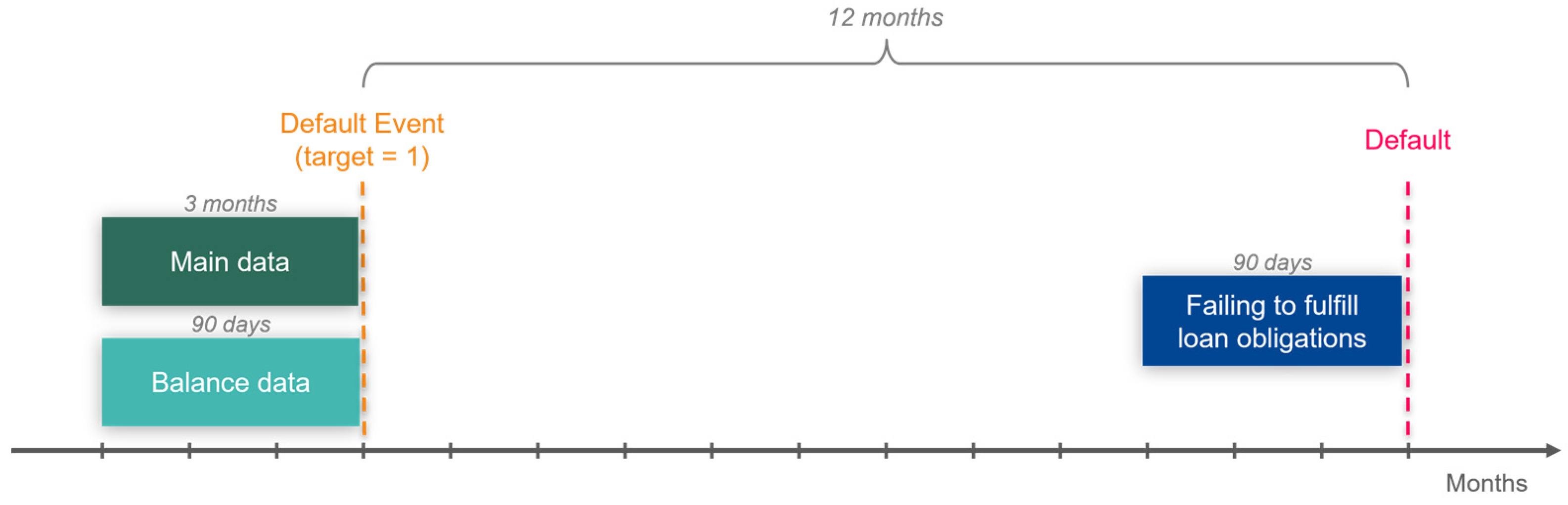
4.1.1. Data Filtering

As the data contains a large number of observations per customer, it is necessary to filter out noise. Figure 2 shows the overall strategy for selecting these observations. The customer is defined to be in legal default after having failed to fulfil its loan obligations for 90 days, shown as the pink line in the figure. The objective is to predict such legal defaults occurring within the next 12 months, as shown with the stapled orange line. For the remainder of the text, we define this as a default, unless otherwise specified. Thus, all observations after a default are irrelevant for predicting legal default, and consequently, removed for all defaulting customers.

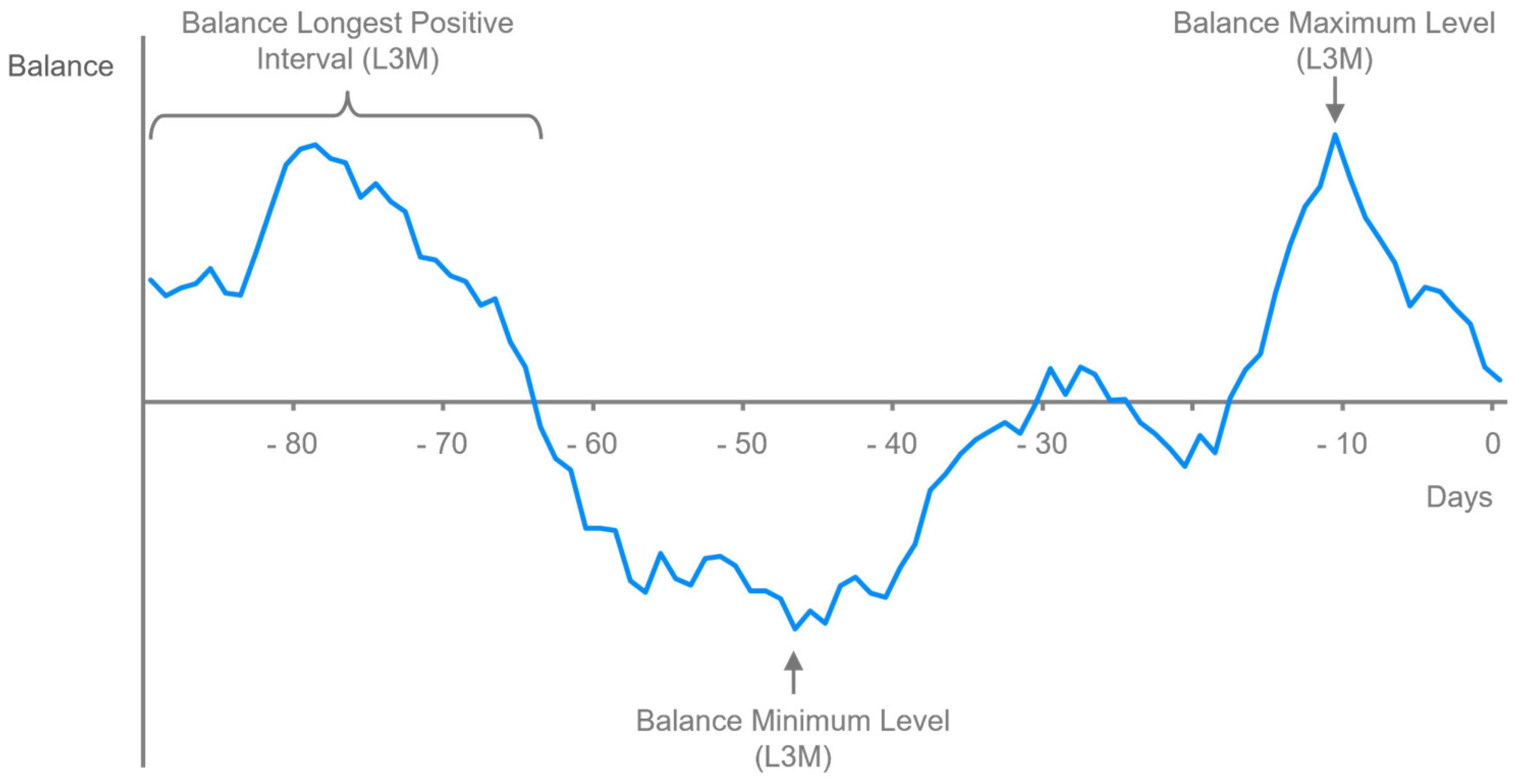
4.1.2. Feature Extraction

Several aggregation measures were implemented on the filtered data to extract signals from the data. These aggregation measures differed between the mainfile and the balancefile.

A pivot transformation was applied to the mainfile. This transformation is illustrated in

Table 2. Illustration of the pivot transformation used on the mainfile dataset. xⁱ_j represents an observation (array of feature values) for customer j at time i, where i = 0 indicates the last observation present in the data. Observe how customer A has four consecutive rows of data, and thus no NaN values after the transformation, whereas customer B misses an observation at time T − 1 and thus has NaN values for the lags of 1.

(A) Before Pivot Transformation
Date	Id		Features
30.9	A		x0A
31.8	A		xA1
31.7	A		xA2
30.6	A		xA3
31.5	B		x0B
31.3	B		xB2
28.2	B		xB3
31.7	C		xC0
(B) After pivot transformation
Date	Id	Current	Lag 1	Lag 2
30.9	A	x0A	xA1	xA3
31.5	B	x0B	NaN	xB3
31.7	C	xC0	NaN	NaN

, where the original data is converted to a format with one row per customer, i.e., a matrix with 13,969 rows. The new table is built around the last observation of each customer, following the description above. In the pivot operation, one- and three-month lags were utilized. There are two reasons why a customer might have its last observation at time $T$; either it enters a default at $T+1$ or there are no subsequent observations for the customer in the data. Either way, the final dataset will include features captured at time $T$ and the lagged features from $T-1$ and $T-3$. Note that, in the pivot transformation, missing observations are preserved to ensure consistency between the observations. Hence, if the mainfile has a customer with only one observation, as is the case for new loan applicants, NaN values are generated for the lagged features.

In order to capture the development leading up to the last observation, several functions were applied to the lagged features, thus further increasing the feature space. In addition to including the still features, shown in Table 2B, both the actual difference in feature values and the percentage changes in the feature values for the lagged features were included in the pivot transformation.

A different set of aggregation measures was applied to the balancefile. Based on each customer’s balance movements over the last 90 days, we generated five new features, and three of them are visualized in Figure 3. The new features represent the standard deviation, maximum value, and minimum value over the entire period. The purpose of adding these features is to obtain deeper insights into the customer’s economic situation and financial stability. In addition to the information provided by these three features, we wanted to derive a measure indicating financial distress. Based on the assumption that distressed customers will struggle to remain balance-positive for long periods, we designed a “distress feature” capturing the longest coherent period with a positive balance. Finally, the fifth and last feature generated based on the balancefile dataset captures irregularly large deposits by measuring the difference between the largest and the second-largest jump in the balance. There are two reasons why this feature is assumed to be relevant. First, abnormally large jumps in the balance may indicate loan disbursements from other banks, meaning that the feature can uncover worrying signs in an otherwise positive balance. Secondly, a measure of the stability of the income might provide additional insights into the customer’s financial situation. The inclusion of the balance features provides a lot of additional information to the credit scoring models. Furthermore, it incorporates time series data in a way the bank has never done before.

4.1.3. Feature Selection

The resulting dataset from the feature extraction procedures contain 13,969 rows, corresponding to one row per customer. Due to the pivot transformations, this dataset entails more than 100 features. The number of features had to be significantly reduced to make the model more explainable and avoid the curse of dimensionality, i.e., separating the data based on too many features. Features were dropped based on a backward feature selection procedure on a random subset of the data used for training. The resulting dataset eventually used for training and evaluating the LightGBM model has 13,969 rows and 18 features. Further feature explanations, statistics, and distributions are provided in Appendix B.

4.2. Data Preparation for Logistic Regression

The bank provided the LR model used in this study, making it an entirely realistic benchmark model. The target variable of the bank’s model is the same as the default variable used in ours, i.e., predicting the probability of a legal default occurring within the next 12 months. The bank’s LR model utilizes six features, where each feature is split into several bins. Consequently, we created an LR-specific dataset based on a recipe from the bank that was one-hot-encoded to match the categories defined by the bins. To ensure that the LR model and the corresponding dataset complied with the assumptions behind Logistic Regression, we used Variance Inflation Factors (VIF) to verify an acceptable level of multicollinearity among the features and the Box-Tidwell test to check for linearity in log-odds. As the bank has deemed its LR model to be a trade secret, we are prevented from disclosing further details of its inner workings or details of the performed binning operations.

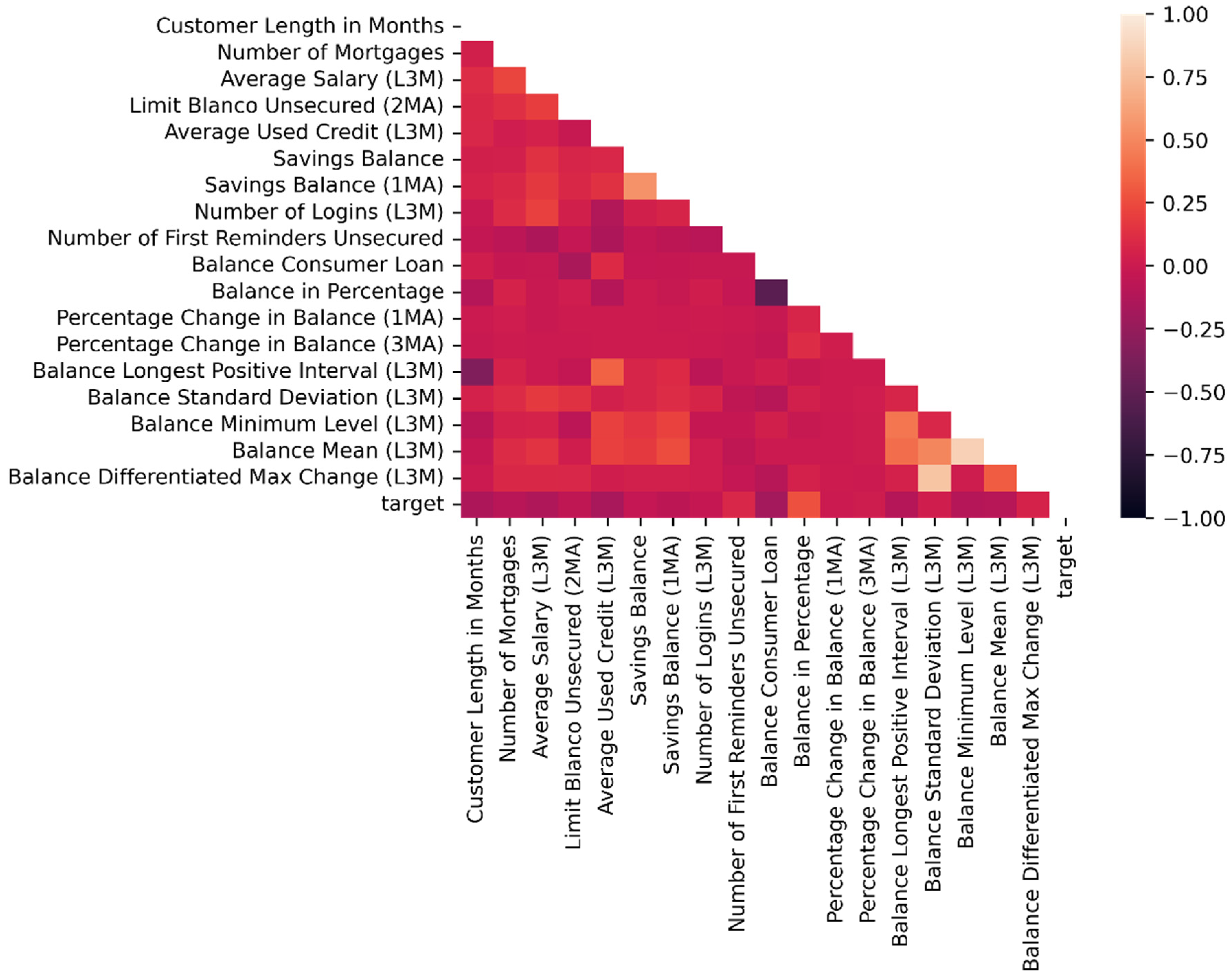
4.3. Data Visualization

Several data visualization techniques were employed to gain additional insight into the nature of the data. These are described in Appendix I.

5. Results

In this section, we present and discuss our findings. We focus on how AI models, such as LightGBM, can advance credit scoring by enabling the models to process more extensive datasets. However, to verify the predictive advantage of LightGBM compared to LR, a second, scaled-down LightGBM model is fitted solely on the features used in the LR model.

Prior to developing the models, the data was split into a training set and a test set using stratified sampling. The test set contained 40% of the original data, corresponding to 5587 customers. The test was completely held out during the development phase as a measure to prevent overfitting and to ensure the validity of the results. Class distributions for the training and test set are found in Appendix B. Stratified k-fold cross-validation was further used to optimize the training on the training set.

Neptune-Optuna client (Niedzwiedz 2022) was used to perform hyperparameter searches for the LightGBM model. The resulting hyperparameters from the best performing trial used in the final model can be found in Appendix D.

The performances of the models were evaluated using ROC and PR curves, with their corresponding area under the curve (AUC) values. One of the advantages of using these evaluation metrics, is that they are not constrained to thresholds for classifying default or non-default. Hence, ROC AUC and PR AUC provide an aggregated performance measure across all possible classification thresholds. The metrics are further explained in Appendix E.

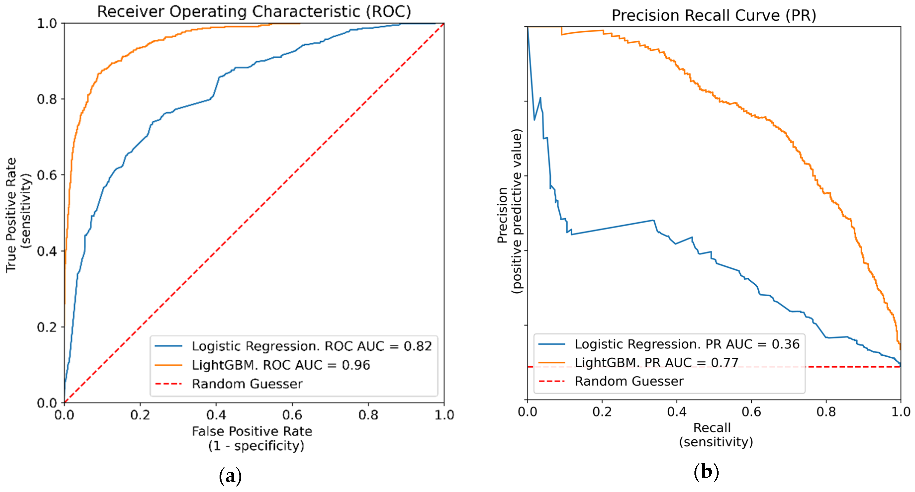
5.1. Model Evaluation

Table 3. Confusion matrix for different thresholds for the LightGBM and Logistic Regression models.

		LightGBM		Logistic Regression
	Actual	Positive	Negative	Positive	Negative
	Predicted
Threshold = 10%	Positive	467	1170	464	3255
	Negative	25	3926	28	1841
Threshold = 15%	Positive	455	927	438	2524
	Negative	37	4169	54	2572

shows confusion matrices comparing the performance of the LightGBM model and the Logistic Regression model. For the LightGBM model with a threshold of 10%, the value of 467 represents the number of true positives, 1170 is the number of false positives, 25 is the false negatives, whereas 3926 represents the true negative values. Note that the table includes the thresholds 10% and 15%. Using a probability of default (PD) threshold of 10% means that any customer with PD higher than 10% is classified as defaulting, and any customer with lower or equal PD is classified as not defaulting. Thus, from a practical perspective, lower thresholds correspond to stricter models as fewer loans are granted. From the table, we can see that at the strictest level (threshold = 10%), the LightGBM model is able to capture more customers subject to default yet still achieves a higher precision (fewer false positives).

Figure 4 provides the ROC and PR curves for both the LR model and the LightGBM model. Both models perform well measured ROC AUC, with scores above 0.8, thus indicating strong predictive capabilities. It is evident from both plots, however, that the LightGBM model outperforms the LR model for all thresholds, with an area under the LightGBM curve (orange) of 0.96 compared to 0.82 for the LR model (blue). The difference constitutes a 17% improvement in ROC AUC for the LightGBM model. The findings in Table 3 and Figure 4 clearly show the advantage of the LightGBM model, as it outperforms the benchmark LR model for all thresholds. Further evaluation metrics, confirming the edge of LightGBM, are summarized in

Table 4. Metrics for the three models that were trained. LightGBM was trained with 18 features, whereas LightGBM (LR) was used for directly comparing Logistic Regression with LightGBM using the same six features.

	Metric	LightGBM	LightGBM (LR)	Logistic Regression
Threshold = 10%	F1-score	43.90%	26.00%	22.00%
	Recall	94.90%	97.00%	94.30%
	Precision	28.50%	15.00%	12.50%
	Accuracy	78.60%	51.40%	41.20%
Threshold = 15%	F1-score	48.60%	29.10%	25.30%
	Recall	92.50%	95.10%	89.00%
	Precision	32.90%	17.20%	14.80%
	Accuracy	82.80%	59.10%	53.90%

. Other authors also find that AI models outperform LR models both in credit default prediction and explicability. Bussmann et al. (2020b), inform that their best XGBoost model attains an AUROC of 0.96, strongly outperforming their LR benchmark model, which attains an AUROC of 0.81. Ariza-Garzón et al. (2020) concludes that credit risk machine learning approaches may outperform statistical approaches, such as logistic regression, in terms of not only classification performance but also explainability. Other authors cited in this study obtain similar results.

LightGBM Model Based on LR Features

A second, scaled-down LightGBM model was created to confirm the predictive advantage of LightGBM compared to LR. This model used the same six features as the LR model to make the comparison as realistic as possible. Note that these features were not binned as in the LR model but used directly. The scaled-down LightGBM version still outperformed the LR model, achieving an ROC AUC of 0.89, corresponding to a 9% increase. Results from this model are shown in Table 4 as LightGBM (LR). Further comparison figures, such as ROC AUC and PR AUC curves, are found in Appendix F.

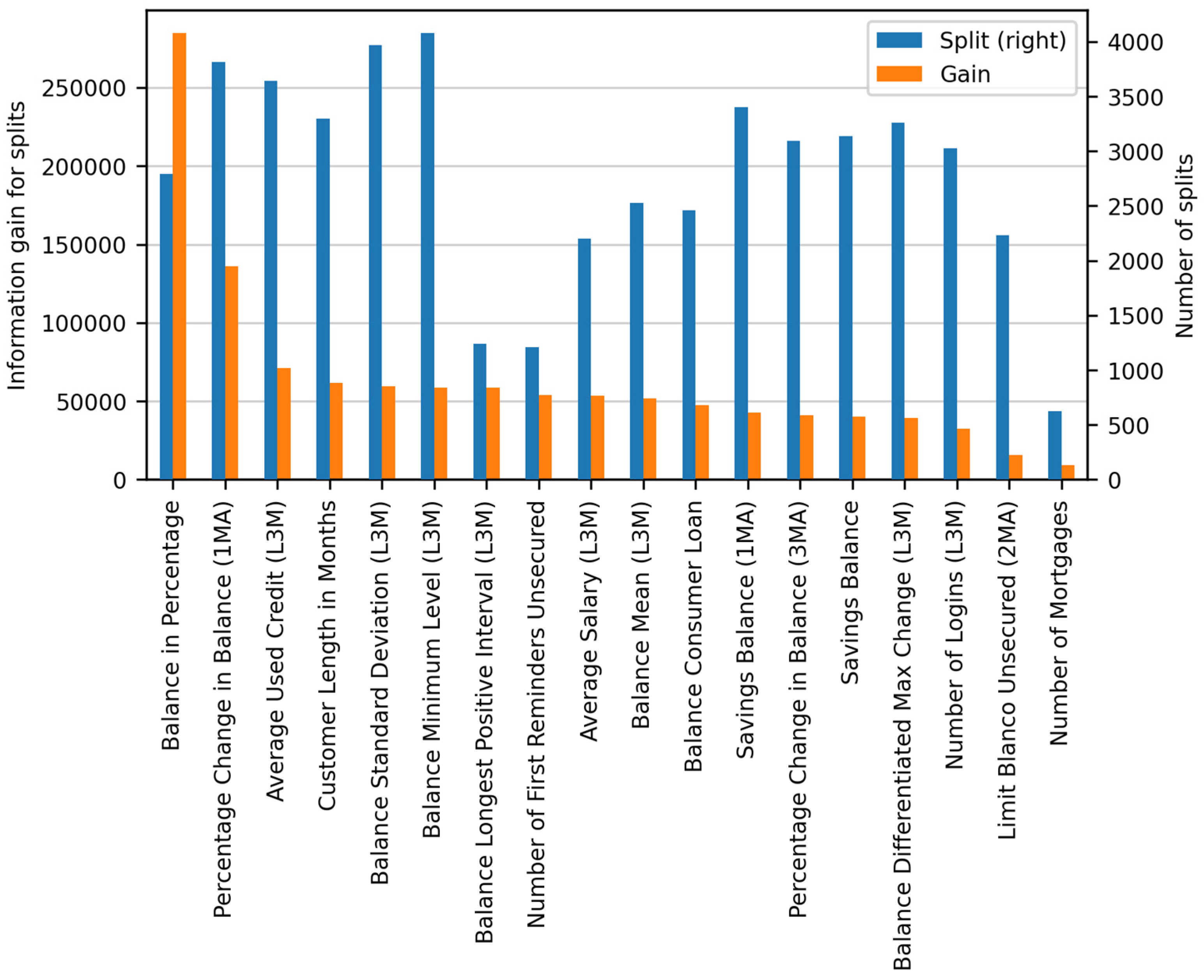
5.2. LightGBM Explainability

Figure 5 shows the feature importance in the LightGBM model. Note that, in order to obtain the splits and gains for the entire LightGBM model, we averaged the feature importance across the ten individual models resulting from cross-validation. In the plot, blue bars indicate the total number of splits on each feature, whereas orange bars indicate the total information gains of splits that use the feature. From the plot, it is clear that Balance in Percentage and Percentage Change in Balance (1MA) are the two features associated with the highest information gain. It can also be observed that Balance Minimum Level (L3M), Balance Standard Deviation (L3M), and Percentage Change in Balance (1MA) are the features with the largest number of splits in each node. Besides being only a proxy for average feature effects on the dependent variable, a clear disadvantage of LightGBM explainability plots is the lack of directional feature effects. The high information gain of Balance in Percentage indicates that it is an important feature for separating the two classes in the dataset. However, it is impossible to interpret to what extent the feature would impact a given prediction. This information is not provided by the number of splits either, as this only measures the number of times each feature is used in the model. There is clearly a need to improve the explainability of LightGBM, and the following section shows how this can be achieved using SHAP.

5.3. SHAP Explanations

SHAP values correspond to feature effects. As outlined in Section 3.5, SHAP values are calculated using a conditional expectation function derived from the LightGBM model. However, the 10-fold cross-validation of the LightGBM model complicates the application of SHAP, as SHAP expects one single model as the input. To overcome this issue, we averaged the SHAP values of the ten individual models, in line with the recommendations of the creator of SHAP (Lundberg 2018).

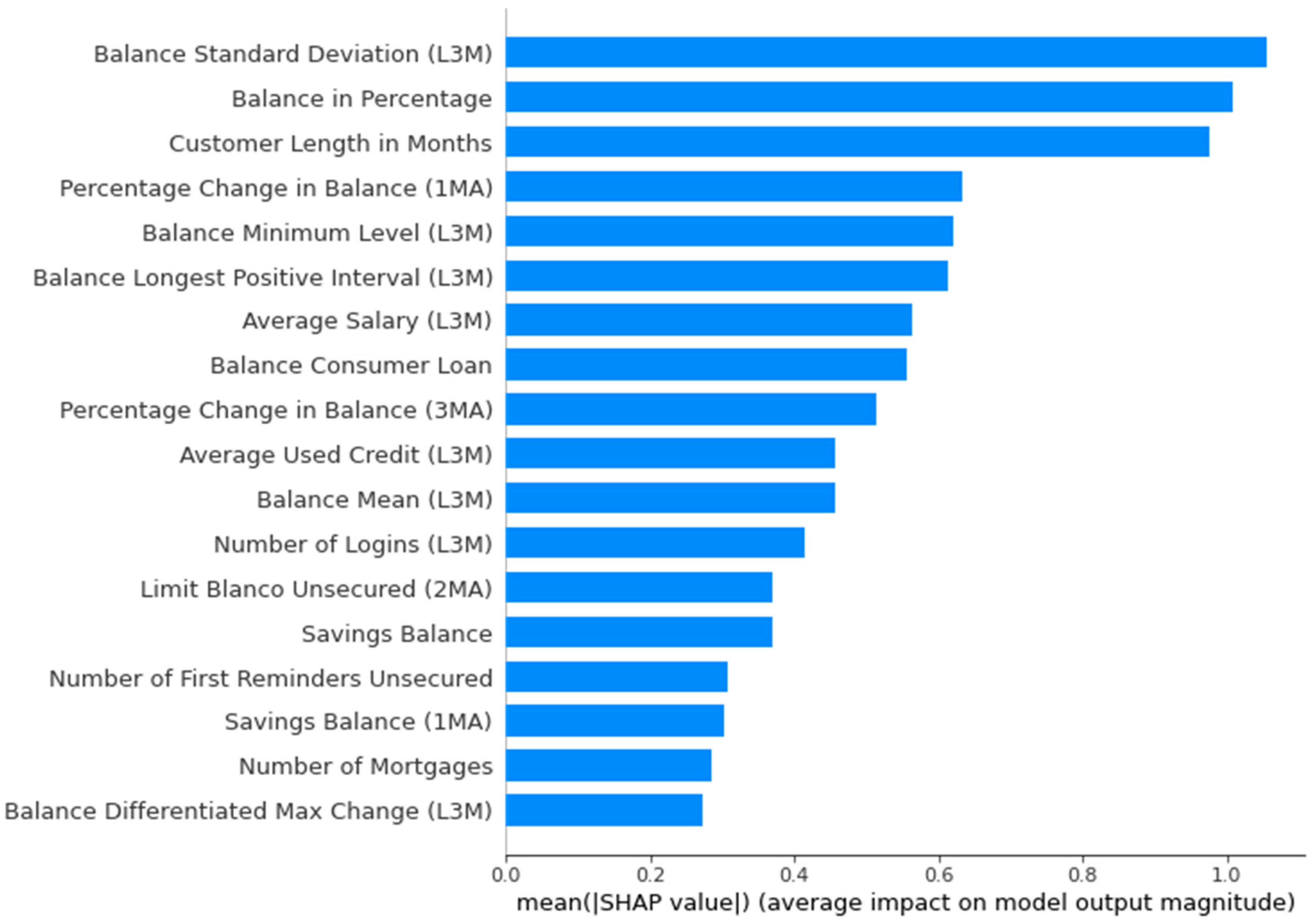
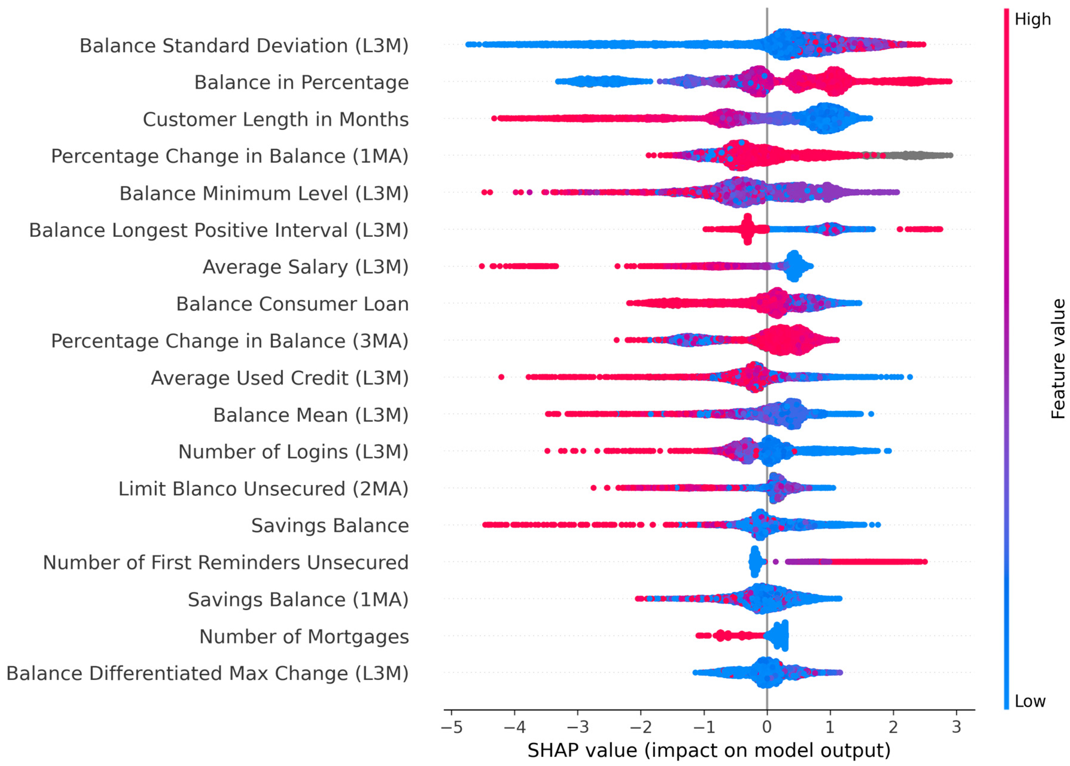
5.3.1. Global Explanations

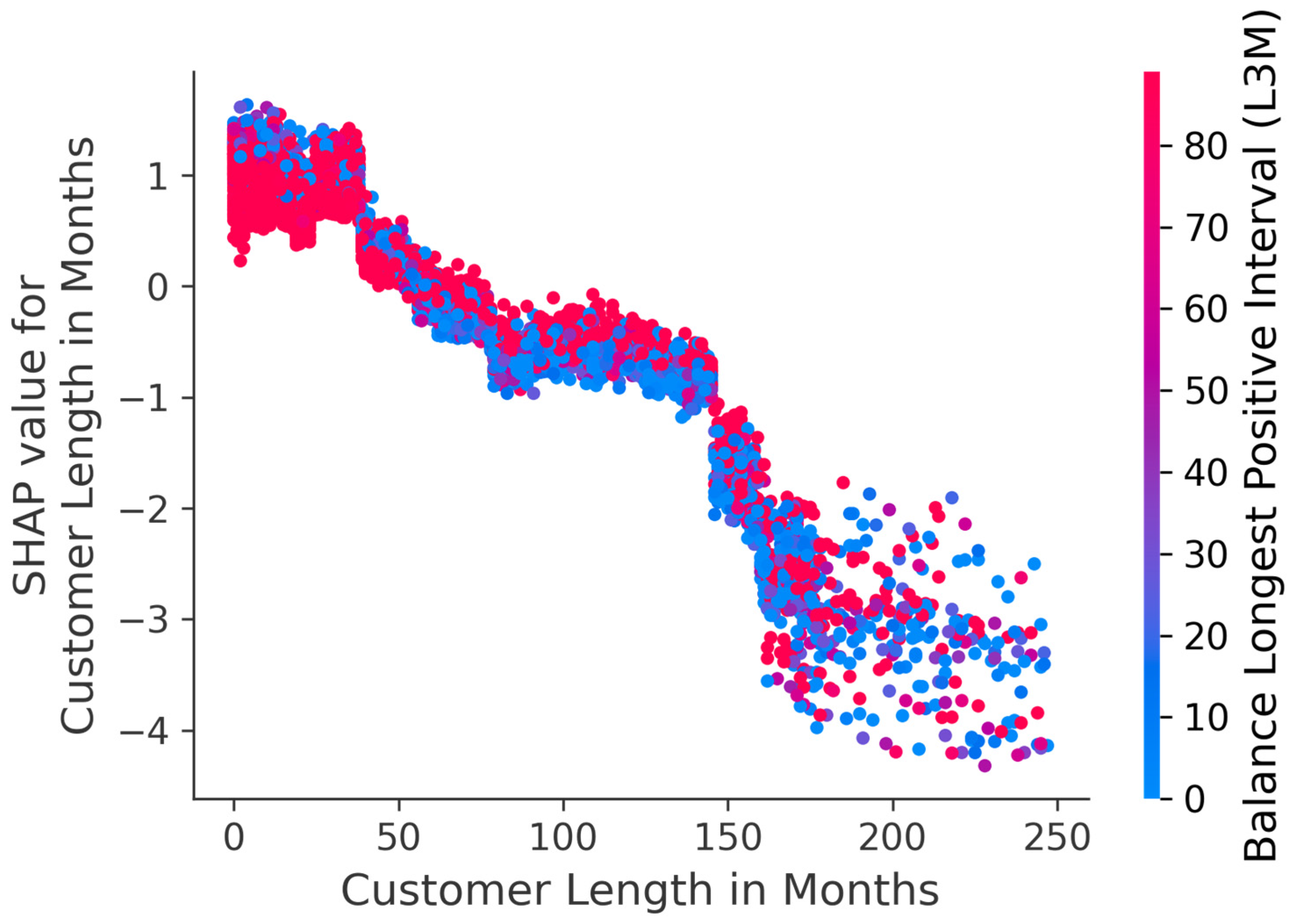
Figure 6 shows the magnitude of the contribution of each feature, measured in absolute log-odds values. We observe that Balance Standard Deviation (L3M), Balance in Percentage and Customer Length in Months have the highest impact on the model. The feature effects found by SHAP correspond reasonably well with the LightGBM importance plot in Figure 5, as many of the same features show significant importance measured in either splits or gain. Furthermore, we can observe that features from the balance dataset are of high importance. This clearly indicates that utilizing daily account movements for credit scoring customers gives the model more signal, thus increasing its predictive performance.

Figure 7 shows a more detailed summary of the workings of the LightGBM model, where directional feature effects on the resulting predictions are visualized. Each dot on the feature row represents a single instance in the dataset, distributed on the x-axis according to the SHAP value for that feature value. The high and low relative feature values are color-coded as red and blue, respectively. Missing values are colored grey. High SHAP values are associated with an increase in the predicted probability of default, whereas low SHAP values correspond to a reduction in the predicted probability of default. The features are ranked by importance, with the most important features for the prediction at the top.

Most of the feature rows in Figure 7 display a distinct trend in how different feature values affect the model. In other words, one can observe a clear distinction between the red and blue dots, as high and low feature values contribute in different directions in terms of default probability.

Dependence Plot

Contrary to LR, LightGBM can utilize complex cross-feature relations in its black box calculation. SHAP can visualize this by plotting all instances in a scatter plot, with the feature value on the x-axis and the importance measured in SHAP values on the y-axis. By color-coding the values of a second feature, the plot can then display dependencies between variables and how they affect the model. The insights from such dependence plots can provide valuable information for banks and regulators about the inner workings of AI models and thus help evaluate whether the model abides by the regulatory requirements described in Section 2.

Figure 8 shows how the SHAP values, and thus the feature effects, for Balance Standard Deviation (L3M) vary for different feature values. Note that the data is not normalized. The upward trend in the plot indicates that higher volatility in a customer’s balance over the last 90 days is associated with an increase in default probability. Standard deviations below approximately 2000 are associated with negative SHAP values, meaning that these feature values contribute to nondefault. In the range between approximately 2000 and approximately 30,000, the SHAP values increase steadily, denoting that the importance of the Balance Standard Deviation (L3M) feature as an indicator of default increases. Above 30,000, the plot is significantly sparser as few customers experience such high levels of volatility in their balance.

The SHAP dependence plot can be further extended by color-coding interaction effects between features. This is displayed in Figure 9, where the SHAP values of Customer Length in Months are displayed and colored based on the feature values of Balance Longest Positive Interval (L3M). A clear trend is visible. Longer customer relationships with the bank are associated with a lower probability of default. Furthermore, a few larger shifts in the effect on the probability of default are visible. For instance, customer relationships shorter than approximately four years (48 months) contribute to default (positive SHAP values), whereas relationships longer than approximately 12 years (144 months) are very positive in terms of creditworthiness (large negative SHAP values). More mature customers are thus less likely to default on their loans.

However, the vertical spread in the plot indicates that other features interact with Customer Length in Months. For customer lengths below 150, the vertical separation of the color-coding suggests that Balance Longest Positive Interval (L3M) is one among these variables. For customers with longer continuous positive balances (red dots), the feature effect of customer length on default is reduced, as the red dots tend to lie closer to a SHAP value of zero. However, for customers with a shorter continuous positive balance (blue dots), the effect of customer length is more important for default prediction, as the absolute SHAP values are larger. This pattern ends for customer lengths above 150, indicating that other features have more significant interaction effects with Customer Length in Months for these instances.

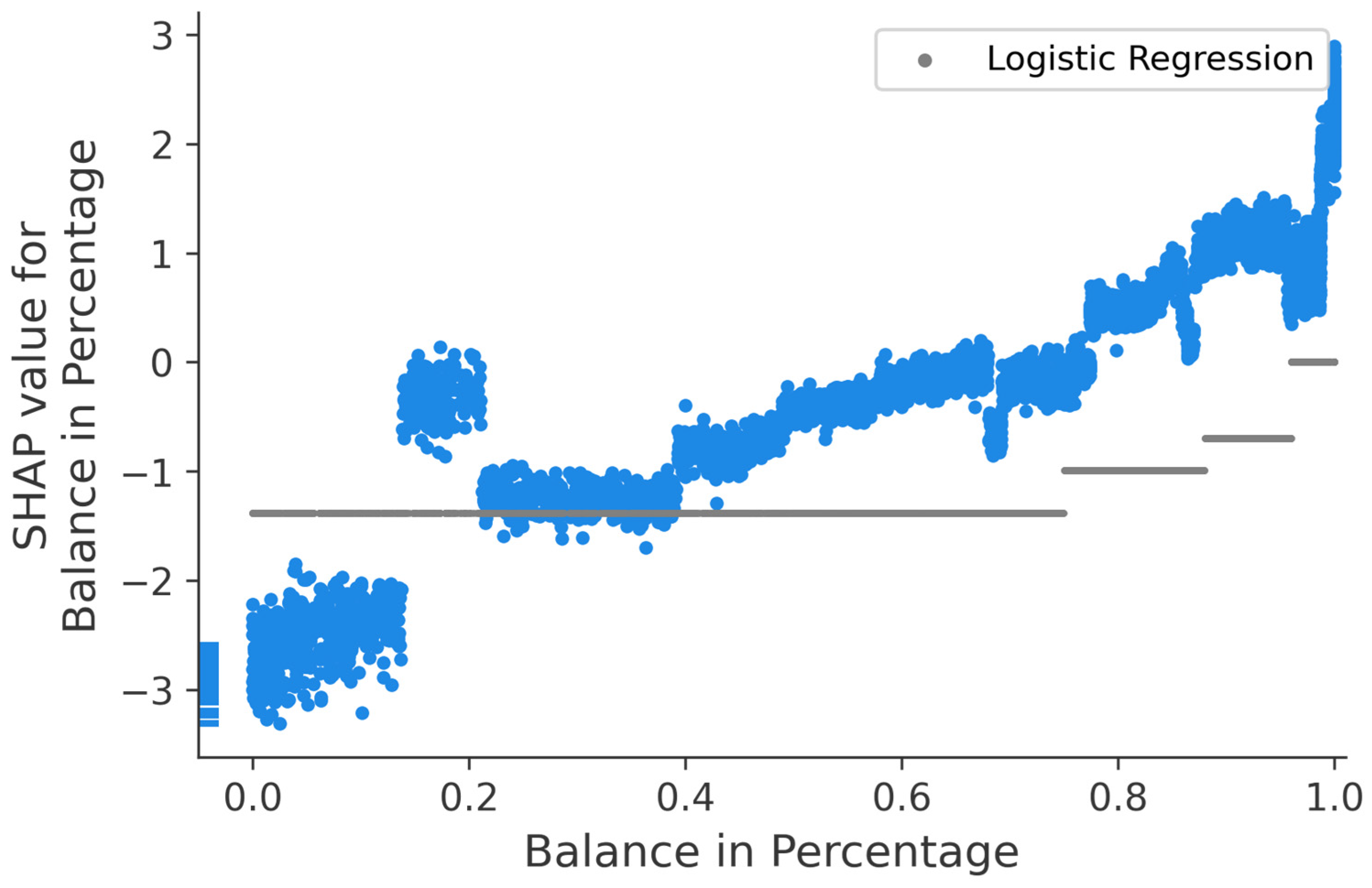
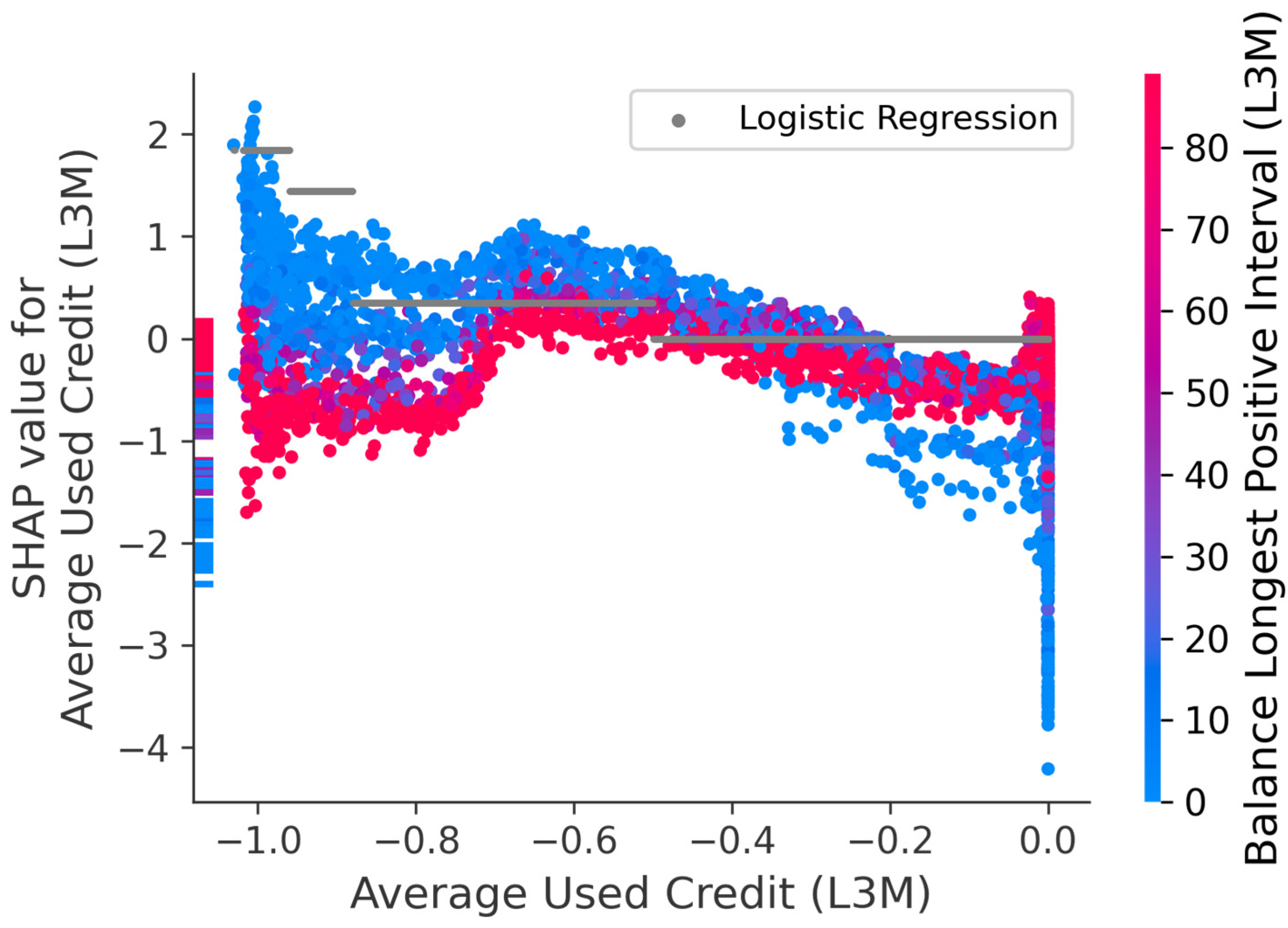
Dependence Plot with Logistic Regression Coefficients

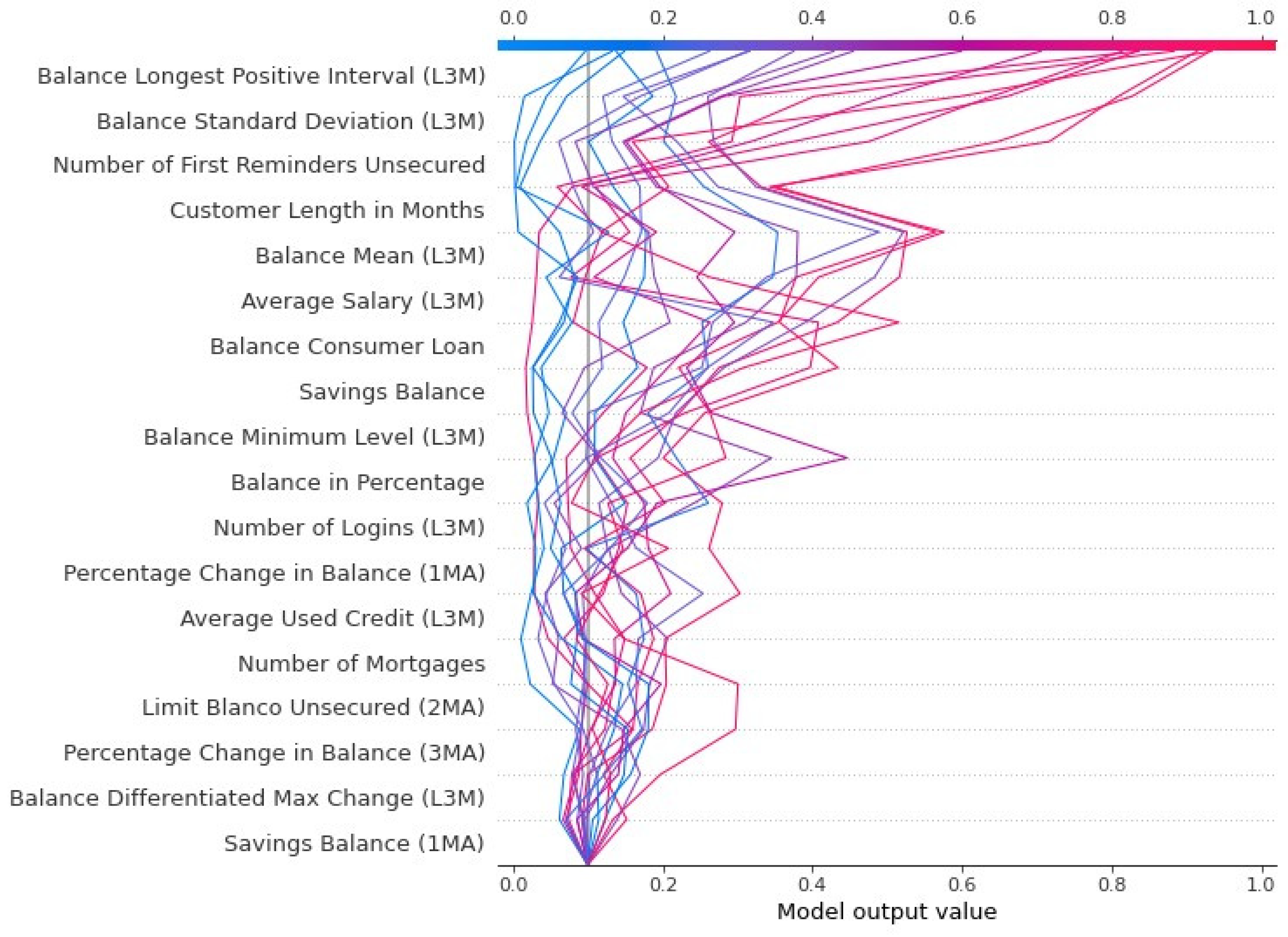
In the following subsection, we offer a novel way of comparing the SHAP feature effects with the feature effects in the LR model. The LR dependencies were derived using the coefficient of the features and mapping the binned values back to the original values to use the same x-axis. The result is visualized with grey dots in the figures. This approach can show where the feature effects differ between the models and provide insights as to why one model outperforms the other.

Figure 10 combines a SHAP dependency plot with an LR dependency plot for the Balance in Percentage feature. This feature measures the percentage share of the issued consumer loan that the customer has outstanding at the time of credit scoring. Specifically, a feature value of 0.0 means that the customer has repaid all its debt, while a value of 1.0 implies that all the debt is still outstanding. The leftmost dots in the plot, next to the y-axis, represent missing feature values in the dataset provided by the bank and correspond to the gray dots in Figure 7.

Both the SHAP and LR graphs display an upward-sloping trend, where higher feature values are associated with a higher probability of default. Comparing the two graphs plotted in Figure 10, one can observe that the magnitude of the SHAP feature effects is greater than the LR model’s feature effects on both ends of the x-axis (further away from y = 0). Thus, the LR model appears to underestimate the effects of the Balance in Percentage feature, though it is able to capture the overall trend of the effects. For instance, the LR model assigns the same negative contribution for all feature values below approximately 0.75. The straight grey LR line shows this. The LightGBM model is able to differentiate this group of customers substantially. LightGBM clearly finds segments where the customers with outstanding consumer loans lower than approximately 17% have notable negative SHAP values, indicating significant creditworthiness. The difference between the models is also visible for the largest feature values. For example, for customers with outstanding consumer loans over 95%, LightGBM and SHAP yield a significantly higher probability of default than the LR model. Overal, the LightGBM model’s advantage in its ability to differentiate customers based on the Balance in Percentage feature can be a part of the explanation of why the model significantly outperforms the LR model.

An example where the feature importance of the LR model coincide better with the SHAP values is shown in Figure 11. The figure contains both SHAP and LR dependence plots for Average Used Credit (L3M). The feature measures the average share of the granted credit limit for unsecured products drawn in the last three months. Drawn credit is defined as a negative number and credit limit as a positive number, meaning that feature values of −1.0 and 0.0 indicate that the credit facilities have been fully drawn and remained untouched, respectively.

Average Used Credit (L3M) feature values below −0.9 contribute substantially to increasing the probability of default in the LR model. The effects are more ambiguous in the LightGBM model, as the vertical distribution of the SHAP values ranges from −1 to +2, indicating that other variables might interact with this feature. From the color coding, it is evident that the interaction effect between Average Used Credit (L3M) and Balance Longest Positive Interval (L3M) can help to explain the spread. Among customers who have drawn most of their credit facilities (feature values below approximately −0.7), those with a shorter period of continuous positive balance (blue) are far more likely to default than those with longer positive stretches (red). For the latter, the default probability is actually reduced, meaning that a combination of a low feature value for Average Used Credit (L3M) and a high Balance Longest Positive Interval (L3M) is an indicator of creditworthiness. The LR model’s inability to detect such multidimensional relationships between features makes it fundamentally inferior to advanced AI models, thus explaining some of the deficit in predictive utility.

Decision Plot

Figure 12 can provide further insights into why LightGBM outperforms the LR model. The plot shows the feature effects of 20 instances that go into default. These instances are wrongly classified as non-default by the LR model, but correctly classified as default by the LightGBM model. The features on the y-axis are ordered by descending importance, whereas the upper x-axis shows the LightGBM predictions on these instances. The colors of the lines indicate the predicted probability of default; red indicates strong confidence in default, whereas blue indicates lower confidence. Moving from the bottom to the top of the plot, one can observe that each feature’s effects on the resulting prediction are added to the intercept. The intercept, represented as the gray vertical line in the plot at 10%, is the chosen cutoff for predicting default versus non-default. The value was selected as 10% as it represents the sum of the true proportion in the test class (8.8%), plus a small risk margin.

As we can see from the upper x-axis in Figure 12, the model displays a wide range of default probabilities among the 20 customers. The predictions vary from 0.9 to 0.1 and are color-coded accordingly. The SHAP feature effects show that most of the differences in PD are caused by the four most important features, as one can observe a large spike in the predicted probabilities of the red lines for the upper four features. For almost all instances, the balance features Balance Longest Positive Interval (L3M), Balance Standard Deviation (L3M) and Balance Mean have an elevating effect on the PD. This effect means that these three variables contribute significantly to the LightGBM model’s correct default predictions. Since the Logistic Regression model is created without the balance features, this might explain why the LightGBM model correctly classified these instances as default, whereas LR did not.

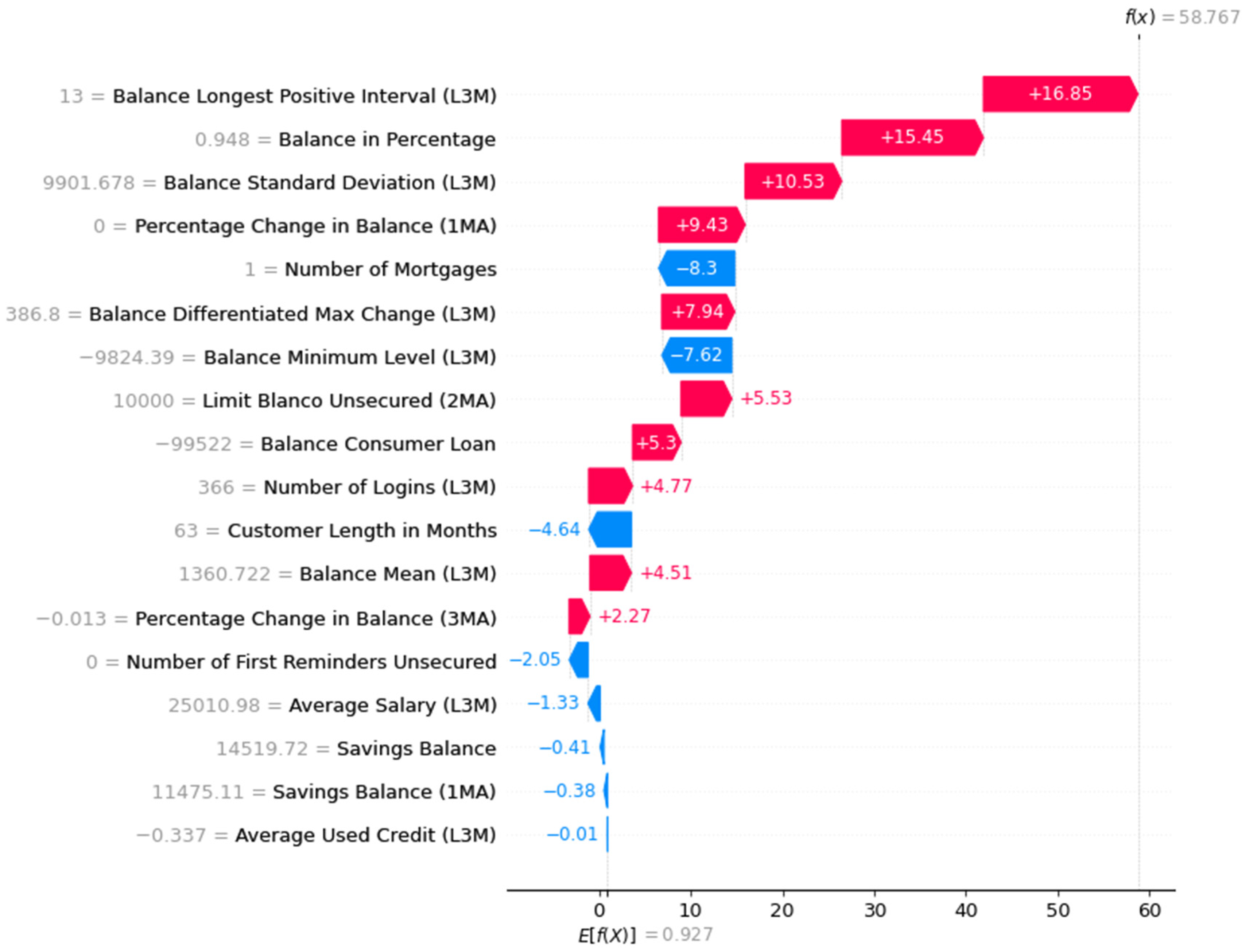
5.3.2. Local Explanations

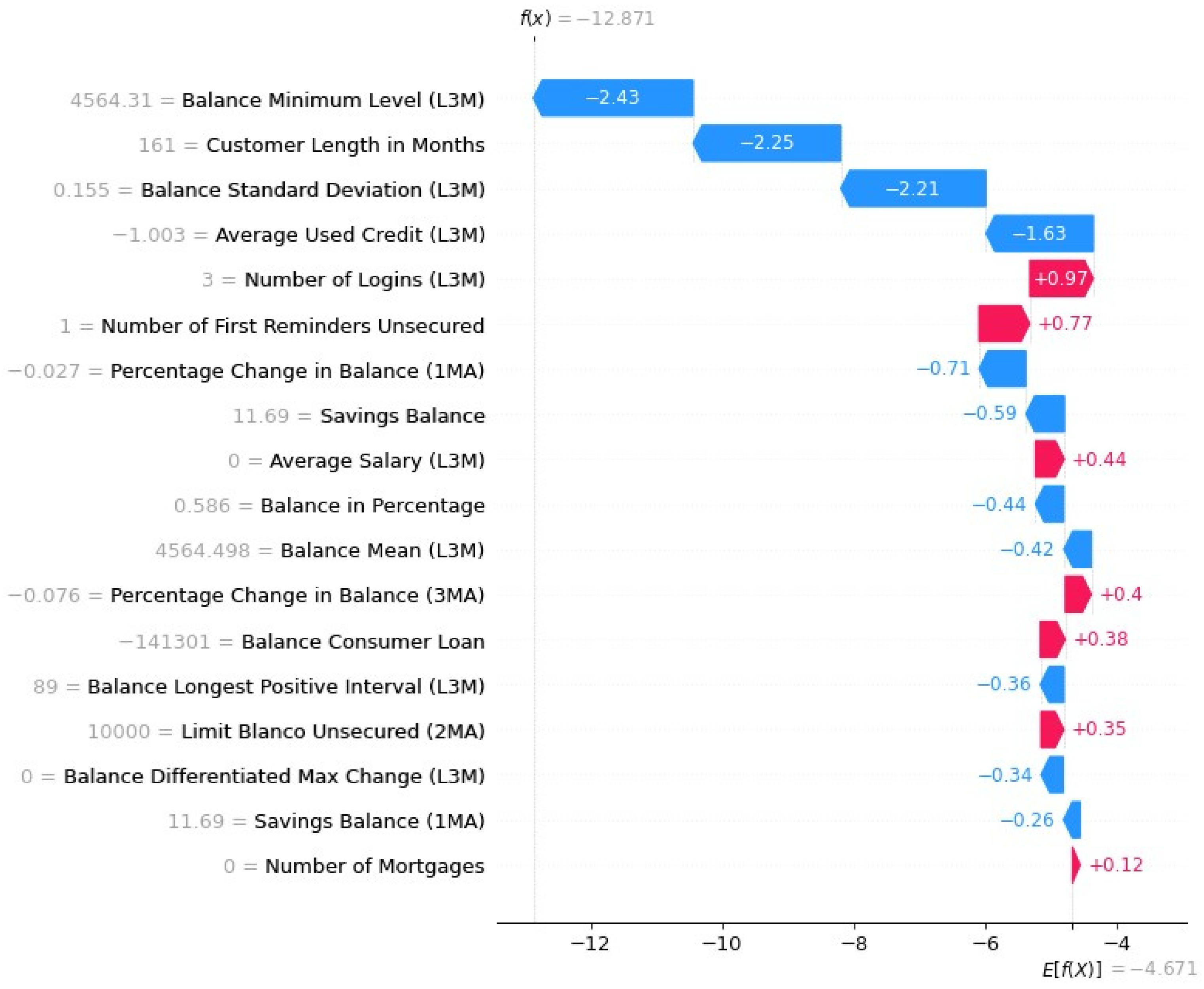
Waterfall Plot

SHAP can further provide descriptive and intuitive explanations for individual predictions through waterfall plots. The SHAP waterfall plots show the contribution of each feature value to the default prediction, with red and blue bars indicating positive and negative contributions, respectively. The features are ranked by importance, and the actual feature values are displayed on the left side. In Figure 13, the prediction by the LightGBM model is displayed as $f\left(x\right)$ and the positive bias or intercept from the LightGBM model is expressed below the plot as $E\left[f\left(x\right)\right]$, both measured in log odds.

The feature value contributing the most to this particular non-default prediction is the Balance Minimum Level (L3M) of 4564, showing that constantly having a positive balance is an important indicator of creditworthiness in the LightGBM model. The second most decisive contribution comes from the Customer Length in Months value of 161. The negative contribution of −2.25 reflects the findings in Figure 9, where customer relationships longer than 144 months display a significant reduction in the probability of default. The depicted customer is further part of the low-risk group with a stable economic situation identified in Figure 8, exhibiting a Balance Standard Deviation (L3M) as low as 0.155. The last major contributor to non-default is the Average Used Credit (L3M) feature value of −1.003. It is interesting that having over-drawn the credit facilities actually contributes towards a nondefault prediction for the customer in the LightGBM model. This differs from the LR model, where Figure 11 shows that such low feature values elevate the PD significantly. However, because the customer has a high Balance Longest Positive Interval (L3M) value, the LightGBM model considers the combination of these features to have a positive impact on the creditworthiness of the customer. The ability to capture such complex feature interactions showcases one of the important strengths of the LighGBM model.

Waterfall Plot with Probabilities

The explainability of the SHAP waterfall plots can be further improved by converting the feature effects from log-odds to probabilities.

An example of SHAP waterfall plots with probabilities is shown in Figure 14, where we see that the predicted probability of default, $f\left(x\right)=58.8\%$, equals the sum of the SHAP values in probabilities, and the expected probability of default from the model, $E\left[f\left(x\right)\right]=0.9\%$.

The instance in Figure 14 represents a customer correctly identified as defaulting by the LightGBM model but predicted not to default by the Logistic Regression model. The plot clearly shows that the features from the balance dataset are important; Balance Longest Positive Interval (L3M), Balance in Percentage and Balance Standard Deviation (L3M) increase the probability of default with approximately 17%, 15%, and 11%, respectively. These features correspond with the most important features found in the decision plot in Figure 12. The feature effects of the SHAP waterfall plots with scaled probabilities are intuitive and easy to understand, making them suitable for explaining model outcomes to non-practitioners.

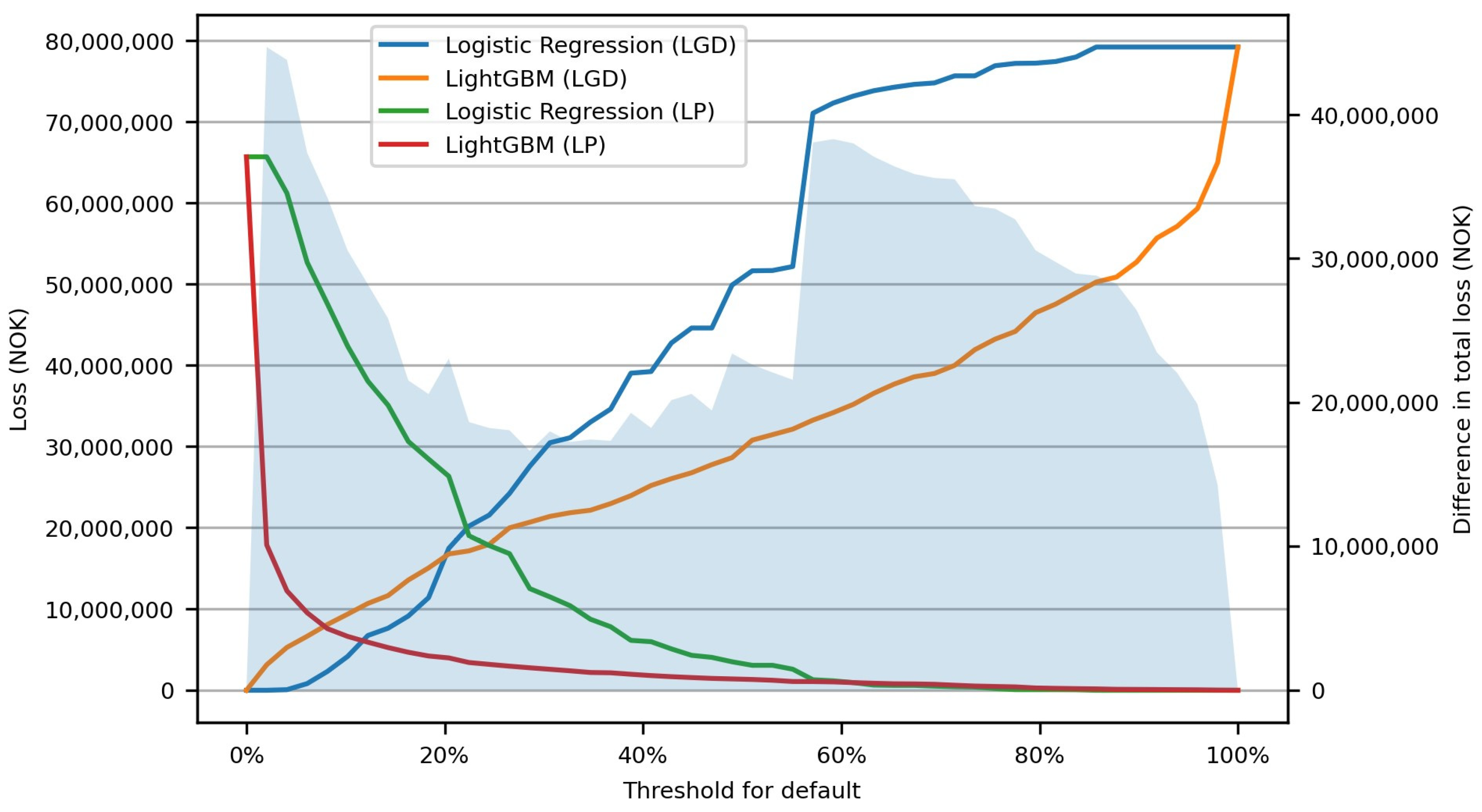
5.4. The Economic Value of a More Accurate Model

This section analyzes the potential economic value of the LightGBM model’s increased predictive performance compared to the bank’s LR model.

For this purpose, we created two evaluation metrics: LGD and LP. LGD represents loss-given-default and is the associated loss from customers who received a loan but defaulted (false negatives). This metric was calculated as a proxy by assuming that all remaining balance is lost on default. LP represents lost profits and is the yearly alternative cost of not granting loans to non-defaulting customers (false positives). LP was calculated by assuming a flat 10% yearly interest rate on all consumer loans. A separate, three-dimensional LP plot, which includes changes in interest rates, is provided in Appendix G.

Figure 15 shows LGD (loss-given-default) and LP (lost-profits) for both models for various probabilities of default thresholds (x-axis). The left y-axis indicates the losses for LP and LGD, whereas the right y-axis indicates the total loss of having an imperfect model. As we can see from the figure, the losses from the LightGBM model are lower than Logistic Regression for both LP and LGD at almost all thresholds higher than 20%. Below 20%, the losses from the LP of Logistic Regression are significantly larger than those from the LP of LightGBM. This plot assumes that the default threshold is equal for both models. Further details are provided in Appendix H.

Despite being an approximated figure, Figure 15 indicates that bank losses can be substantially reduced by enabling AI in credit scoring. As the current effective interest rates on consumer loans in Norway typically range between 10% and 25%1, having an internal threshold of default in the bank somewhere between 10% and 20% seems like a reasonable approximation. At these thresholds, the lost profits of the LightGBM model are significantly lower than for the LR model, with a reduction ranging from about NOK 35,000,000 at 10% to 22,000,000 at 20%. This benefit clearly outweighs the slight inferiority of the LightGBM model’s LGD for the same thresholds. The total reduced losses for using LightGBM instead of LR, on the test set, shown as the shaded area with the y-axis on the right-hand side, are between NOK 30,000,000 and 20,000,000 yearly, depending on the threshold for default.

6. Conclusions

The objective of this study was to apply explainable artificial intelligence (XAI) techniques to credit scoring in banking in order to be able to interpret and justify the models’ predictions. We have shown that LightGBM models outperform LR models for credit scoring in terms of both predictive capability and explainability, and that the economic value of the predictive improvement can be substantial.

The main contributions of this paper are:

• Combining monthly customer application data (income, gender, age, etc.) with daily account data (i.e., transactions data)
• Showing why and how LightGBM outperforms the bank’s current Logistic Regression model, predicting default on unsecured consumer loans
• Exploring how XAI can improve interpretability and reliability of state-of-the-art AI models for credit default prediction
• Proposing a method for measuring the economic value of a more accurate credit default prediction model

We further argue that the combination of SHAP and LightGBM has the potential to answer the three challenges highlighted by EBA, previously discussed in Section 1.

• SHAP can ease the challenge of interpreting results

The local explanations provided by waterfall plots show that SHAP provides an intuitive approach for interpreting results.

• SHAP can facilitate managers’ understanding of the credit models

The dependence plots with LR coefficients provide improved comparisons between different credit scoring models, enabling managers to bolster their understanding of the models.

• SHAP can help to justify a model’s results to supervisory authorities

Comprehensive global explanations visualizing feature importance, feature dependencies, and interactions between features enable a detailed understanding of the different features’ impact on the model output.

In addition, the local explanations provided by SHAP enable justifications for individual predictions, which is a regulatory requirement imposed by GDPR (European Union, Parliament and Council 2016).

In closing we mention some potential future improvements to this study, which might further help enabling XAI for credit scoring. Different tree-based models with XAI should be evaluated on various bank data. A constraint on our study is the propriety nature of our data set and the bank’s logistic regression model. The LR model used for comparing our models should be open-sourced facilitating a more comprehensive comparison with LightGBM. This would require a strategic change at the bank. More research on the calibration of LightGBM models should be conducted. Details on our calibration method, demonstrating the significance of calibration for the LightGBM model’s predictive capability, can be found in Appendix H.2. We believe default predictions could be further improved by developing better calibration methods for the LightGBM model.

References

1. Ariza-Garzón, Miller Janny, Javier Arroyo, Antonio Caparrini, and Maria-Jesus Segovia-Vargas. 2020. Explainability of a Artificial intelligenceGranting Scoring Model in Peer-to-Peer Lending. IEEE Access 8: 64873–90. [Google Scholar] [CrossRef]
2. Bartlett, Peter, Yoav Freund, Wee Sun Lee, and Robert E. Schapire. 1998. Boosting the margin: A new explanation for the effectiveness of voting methods. The Annals of Statistics 26: 1651–86. [Google Scholar] [CrossRef]
3. Basel Committee on Banking Supervention. 2006. International Convergence of Capital Measurement and Capital Standards. Available online: https://www.bis.org/publ/bcbs128.pdf (accessed on 1 November 2022).
4. Bastos, João A., and Sara M. Matos. 2022. Explainable models of credit losses. European Journal of Operational Research 301: 386–94. [Google Scholar] [CrossRef]
5. Benhamou, Eric, Jean-Jacques Ohana, David Saltiel, and Beatrice Guez. 2021. Explainable AI (XAI) Models Applied to Planning in Financial Markets. Available online: https://openreview.net/forum?id=mJrKRgYm2f1 (accessed on 1 November 2022). [CrossRef]
6. Bibal, Adrien, Michael Lognoul, Alexandre De Streel, and Benoît Frénay. 2021. Legal requirements on explainability in machine learning. Artificial Intelligence and Law 29: 149–69. [Google Scholar] [CrossRef]
7. Breiman, Leo. 1998. Arcing classifier (with discussion and a rejoinder by the author). The Annals of Statistics 26: 801–49. [Google Scholar] [CrossRef]
8. Brown, Iain, and Christophe Mues. 2012. An experimental comparison of classification algorithms for imbalanced credit scoring data sets. Expert Systems with Applications 39: 3446–53. [Google Scholar] [CrossRef] [Green Version]
9. Bücker, Michael, Gero Szepannek, Alicja Gosiewska, and Przemyslaw Biecek. 2021. Transparency, auditability, and explainability of artificial intelligencemodels in credit scoring. Journal of the Operational Research Society 73: 70–90. [Google Scholar] [CrossRef]
10. Bussmann, Niklas, Paolo Giudici, Dimitri Marinelli, and Jochen Papenbrock. 2020a. Explainable AI in Fintech Risk Management. Frontiers in Artificial Intelligence 3: 26. [Google Scholar] [CrossRef]
11. Bussmann, Niklas, Paolo Giudici, Dimitri Marinelli, and Jochen Papenbrock. 2020b. Explainable Machine Learning in Credit Risk Management. Computational Economics 57: 203–16. [Google Scholar] [CrossRef]
12. Chen, Tianqi, and Carlos Guestrin. 2016. XGBoost: A Scalable Tree Boosting System. Paper presented at the 22nd ACM SIGKDD International Conference on Knowledge Discovery and Data Mining, San Francisco, CA, USA, August 13–17; New York: ACM, vols. 13–17, pp. 785–94, ISBN 1450342329. [Google Scholar]
13. Connelly, Lynne. 2020. Logistic regression. Medsurg Nursing 29: 353–54. [Google Scholar]
14. Davis, Randall, Andrew W. Lo, Sudhanshu Mishra, Arash Nourian, Manish Singh, Nicholas Wu, and Ruixun Zhang. 2022. Explainable Machine Learning Models of Consumer Credit Risk. Available from the Website of the Global Association of Risk Professionals. Available online: https://www.garp.org/white-paper/explainable-machine-learning-models-of-consumer-credit-risk (accessed on 1 November 2022).
15. El-Sappagh, Shaker, Jose M. Alonso, S. M. Islam, Ahmad M. Sultan, and Kyung Sup Kwak. 2021. A multilayer multimodal detection and prediction model based on explainable artificial intelligence for Alzheimer’s disease. Scientific Reports 11: 1–26. [Google Scholar] [CrossRef]
16. EBA (European Banking Authority). 2021. Discussion Paper on Artificial Intelligencefor IRB Models. English. Available online: https://www.eba.europa.eu/sites/default/documents/files/document_library/Publications/Discussions/2022/Discussion%20on%20machine%20learning%20for%20IRB%20models/1023883/Discussion%20paper%20on%20machine%20learning%20for%20IRB%20models.pdf (accessed on 6 November 2022).
17. European Commission. 2021a. Proposal for a Regulation of the European Parliament and of the Council Laying Down Harmonised Rules on Artificial Intelligence (Artificial Intelligence Act) and Amending Certain Union Legislative Acts. English. Available online: https://eur-lex.europa.eu/resource.htAI?uri=cellar:e0649735-a372-11eb-9585-01aa75ed71a1.0001.02/DOC_1&format=PDF (accessed on 9 May 2022).
18. European Commission. 2021b. White Paper On Artificial Intelligence—A European Approach to Excellence and Trust. English. Available online: https://ec.europa.eu/info/sites/default/files/commission-white-paper-artificialintelligence-feb2020_en.pdf (accessed on 11 May 2022).
19. European Union, Parliament and Council. 2016. Official Journal of the European Union. L 119/41. Brussels: European Union, vol. 59. [Google Scholar]
20. Freund, Yoav, and Robert E. Schapire. 1995. A desicion-theoretic generalization of on-line learning and an application to boosting. In Computational Learning Theory. Berlin/Heidelberg: Springer, pp. 23–37. ISBN 978-3-540-49195-8. [Google Scholar]
21. Freund, Yoav, and Robert E. Schapire. 1999. A Short Introduction to Boosting. Journal of Japanese Society for Artificial Intelligence 14: 771–80. [Google Scholar]
22. Gramegna, Alex, and Paolo Giudici. 2021. SHAP and LIME: An Evaluation of Discriminative Power in Credit Risk. Frontiers in Artificial Intelligence 4: 140. Available online: https://www.frontiersin.org/article/10.3389/frai.2021.752558 (accessed on 6 November 2022). [CrossRef] [PubMed]
23. Hess, Aaron S., and John R. Hess. 2019. Logistic regression. Transfusion 59: 2197–98. [Google Scholar] [CrossRef] [PubMed]
24. Hintze, Jerry L., and Ray D. Nelson. 1998. Violin Plots: A Box Plot-Density Trace Synergism. The American Statistician 52: 181–84. [Google Scholar] [CrossRef]
25. Jolliffe, I. T. 1986. Principal Component Analysis and Factor Analysis. In Principal Component Analysis. New York: Springer, chap. 5. pp. 115–28. ISBN 978-14757-1904-8. [Google Scholar] [CrossRef]
26. Ke, Guolin, Qi Meng, Thomas Finley, Taifeng Wang, Wei Chen, Weidong Ma, Qiwei Ye, and Tie-Yan Liu. 2017. LightGBM: A Highly Efficient Gradient Boosting Decision Tree. In Advances in Neural Information Processing Systems. New York: Curran Associates, Inc., vol. 30. [Google Scholar]
27. Lever, Jake, Martin Krzywinski, and Naomi Altman. 2016. Logistic regression. Nature Methods 13: 541–42. [Google Scholar] [CrossRef]
28. Lundberg, Scott M., Gabriel G. Erion, and Su-In Lee. 2019. Consistent Individualized Feature Attribution for Tree Ensembles. arXiv arXiv:1802.03888. [Google Scholar]
29. Lundberg, Scott, and Su-In Lee. 2017. A unified approach to interpreting model predictions. arXiv arXiv:1705.07874. [Google Scholar]
30. Lundberg, Scott. 2018. How to Get SHAP Values of the Model Averaged by Folds? Available online: https://github.com/slundberg/shap/issues/337#issuecomment-441710372 (accessed on 27 November 2021).
31. Misheva, Branka Hadji, Joerg Osterrieder, Ali Hirsa, Onkar Kulkarni, and Stephen Fung Lin. 2021. Explainable AI in Credit Risk Management. arXiv arXiv:2103.00949. [Google Scholar]
32. Molnar, Christoph. 2019. Interpretable Machine Learning. A Guide for Making Black Box Models Explainable. SHAP (Shapley Additive Explanations): chap. 9.6. Available online: https://christophm.github.io/interpretableAI-book/shap.htAI (accessed on 6 November 2022).
33. Moscato, Vincenzo, Antonio Picariello, and Giancarlo Sperlí. 2021. A benchmark of machine learning approaches for credit score prediction. Expert Systems with Applications 165: 113986. [Google Scholar] [CrossRef]
34. Niedzwiedz, Piotr. 2022. Neptune Optuna Hyperparamet Optimization. Available online: https://docs.neptune.ai/integrations-and-supported-tools/hyperparameteroptimization/optuna (accessed on 6 November 2022).
35. Nixon, Jeremy, Michael W. Dusenberry, Linchuan Zhang, Ghassen Jerfel, and Dustin Tran. 2019. Measuring Calibration in Deep Learning. Available online: https://arxiv.org/abs/1904.01685 (accessed on 6 November 2022). [CrossRef]
36. Peng, Junfeng, Kaiqiang Zou, Mi Zhou, Yi Teng, Xiongyong Zhu, Feifei Zhang, and Jun Xu. 2021. An Explainable Artificial Intelligence Framework for the Deterioration Risk Prediction of Hepatitis Patients. Journal of Medical Systems 45: 61. [Google Scholar] [CrossRef]
37. Quinto, Butch. 2020. Next-Generation Artificial intelligencewith Spark: Covers XGBoost, LightGBM, Spark NLP, Distributed Deep Learning with Keras, and More, 1st ed. New York: Apress. ISBN 9781484256695. [Google Scholar]
38. Ribeiro, Marco Túlio, Sameer Singh, and Carlos Guestrin. 2016. “Why Should I Trust You?”: Explaining the Predictions of Any Classifier. arXiv arXiv:1602.04938. [Google Scholar]
39. Shapley, Lloyd S. 1953. Stochastic Games. Proceedings of the National Academy of Sciences 39: 1095–100. Available online: https://www.pnas.org/content/39/10/1095.full.pdf (accessed on 6 November 2022). [CrossRef]
40. Shrikumar, Avanti, Peyton Greenside, and Anshul Kundaje. 2019. Learning Important Features through Propagating Activation Differences. arXiv arXiv:1704.02685. [Google Scholar]
41. Strumbelj, Erik, and Igor Kononenko. 2013. Explaining prediction models and individual predictions with feature contributions. Knowledge and Information Systems 41: 647–65. [Google Scholar] [CrossRef]
42. Yang, Yimin, and Min Wu. 2021. Explainable Artificial intelligencefor Improving Logistic Regression Models. Paper presented at the 2021 IEEE 19th International Conference on Industrial Informatics (INDIN), Palma, Spain, July 21–23; pp. 1–6. [Google Scholar] [CrossRef]
43. Yoo, Tae Keun, Ik Hee Ryu, Hannuy Choi, Jin Kuk Kim, In Sik Lee, Jung Sub Kim, Geunyoung Lee, and Tyler Hyungtaek Rim. 2020. Explainable Artificial intelligenceApproach as a Tool to Understand Factors Used to Select the Refractive Surgery Technique on the Expert Level. Translational Vision Science Technology 9: 8. [Google Scholar] [CrossRef] [PubMed] [Green Version]
44. Young, H. Peyton. 1985. Monotonic solutions of cooperative games. International Journal of Game Theory 14: 65–72. [Google Scholar] [CrossRef]
45. Zhang, Huan, Si Si, and Cho-Jui Hsieh. 2017. GPU-Acceleration for Large-Scale Tree Boosting. arXiv arXiv:1706.08359. [Google Scholar]
Figure 1. Correlation heatmap of the dataset used by the LightGBM model. The feature combinations are color-coded based on the correlation explained by the color scale to the right. Light colors indicate positive correlations.
Jrfm 15 00556 g001
Figure 2. Timeline illustrating the distinction between default and legal default. Ninety days of balance data and three months of main data are used for predicting the probability of a legal default within the next 12 months. A legal default occurs if a customer fails to fulfil its obligations over a period of 90 days.
Jrfm 15 00556 g002
Figure 3. Illustration of three of the new features generated from the balancefile. The last 90 relevant days of accounting information were used for each customer to create aggregated balance features.
Jrfm 15 00556 g003
Figure 4. Evaluation curves. (a) ROC plot and (b) PR plot comparing the performance of the LightGBM and LR model. It is clear that LightGBM outperforms LR with a 17% and a 114% increase in ROC AUC and PR AUC, respectively.
Jrfm 15 00556 g004
Figure 5. Feature importance according to the LightGBM model. Average values across the 10 models from the stratified cross-validation, ranked by information gain. The number of splits on the right y-axis, and corresponding information gain for splits on the left y-axis.
Jrfm 15 00556 g005
Figure 6. Simplified SHAP variable importance plot for the Light-GBM model, ranked by importance. Note that SHAP values are in absolute log-odds.
Jrfm 15 00556 g006
Figure 7. SHAP variable importance plot for the LightGBM model. Positive SHAP values are associated with an increase in default probability. Feature values are color-coded according to the scale on the right side, e.g., a high level of Customer Length in Months, shown in red, is associated with a decrease in default probability, whereas a low feature level, shown in blue, is associated with an increase in the probability of default. Missing values are colored grey, and all SHAP values are measured in log-odds.
Jrfm 15 00556 g007
Figure 8. SHAP dependence plot showing SHAP values for Balance Standard Deviation (L3M), up to the 95th percentile. Each dot represents one customer and positive SHAP values are associated with an increase in default probability.
Jrfm 15 00556 g008
Figure 9. SHAP dependence plot showing SHAP values for Customer Length in Months, color-coded based on the value of the Balance Longest Positive Interval (L3M) feature. Each dot represents one customer and positive SHAP values are associated with an increase in default probability.
Jrfm 15 00556 g009
Figure 10. SHAP dependence plot showing SHAP values for balance in Percentage. Logistic Regression feature effects for the balance are displayed in grey and scaled to log-odds, corresponding to the SHAP values on the y-axis. All values from the four separate Balance in Percentage bins are mapped back to original values to fit the x-axis.
Jrfm 15 00556 g010
Figure 11. SHAP dependence plot showing SHAP values for Average Used Credit (L3M), color-coded based on the value of the Balance Longest Positive Interval (L3M) feature. Logistic Regression feature effects for average used credit is displayed in grey and scaled to log-odds, corresponding to the SHAP values on the y-axis. All values from the four separate Average Used Credit bins are mapped back to original values to fit the x-axis.
Jrfm 15 00556 g011
Figure 12. Decision plot for 20 defaulting observations correctly classified by the LightGBM model but wrongly classified by the LR model. Each line represents one customer. The plot is read bottom-up, starting with the chosen intercept and adding feature effects until each observation’s final prediction is reached. Features are ordered based on importance, in descending order.
Jrfm 15 00556 g012
Figure 13. SHAP waterfall plot visualizing the predicted feature contributions to a non-defaulting customer. All values are in log odds. The prediction by the model, f ( x ) , corresponds to a probability of 0.0003%. The bias of the LightGBM model is displayed as E [ f ( x ) ] .
Jrfm 15 00556 g013
Figure 14. SHAP waterfall plot with feature effects converted to probabilities. E [ f ( x ) ] is the bias of LightGBM, whereas f ( x ) is the prediction of LightGBM for this instance. All SHAP values are transformed to probabilities. Feature values shown on the left-hand side.
Jrfm 15 00556 g014
Figure 15. Approximated costs for imperfect credit scoring models. The x-axis indicates the threshold for default, whereas the left y-axis indicates potential losses. The shaded area displays the difference in total loss between Logistic Regression and LightGBM and is measured on the right y-axis. Loss given default (LGD) and lost profits (LP) are plotted, for both LightGBM and Logistic Regression.
Jrfm 15 00556 g015