1. Introduction
From a finance theory perspective, bank management involves the management of the main balance sheet risks: interest rate risk, liquidity risk, capital risk, and credit risk. Among these, credit risk has long been identified as the most important risk factor with respect to bank performance (
Boffey and Robson 1995). According to
Barboza et al. (
2016), the Basel I and II accords have further strengthened the importance of managing credit risk for financial institutions.
A bank can assess the credit risk for existing customers, usually using credit scoring models developed based on feature-rich datasets, including demographic data and credit history. These models usually perform well when predicting future defaults and non-defaults, mainly due to access to customer credit history, for example, information on past overdue payments, arrears, and overlays. Explanatory variables created on the basis of such information are crucial for developing well-performing credit scoring models that are able to accurately predict future defaults.
Credit history information is usually unavailable to banks when assessing the credit risk of potential new customers, resulting in credit scoring models that typically perform significantly worse than the models for existing customers. Therefore, lack of credit history information of new customers potentially leads to recruiting more customers who will default on their loans in the future and the rejection of more customers with lower risks of defaulting on their loans in the future. Consequently, the lack of access to the credit history of potential customers could result in lower profitability for the bank.
Despite of an upsurge of empirical articles on credit risk management the last decades, little attention has been paid to utilizing simple but easily accessible transaction data for new potential customers. A potential new data source for the credit history of new customers are the Open Banking APIs that banks are required to establish after the implementation of the European Payment Services Directive, PSD2 (
EUR-Lex 2015). According to PSD2, banks are required to make customer transaction data and balances from the last 90 days available to third parties (including other banks) through their Open Banking APIs if permitted by their customers. It is expected that this will increase competition in the banking market by preparing the ground for FinTechs, and thus incentivizing existing banks to develop better credit scoring models to counter the increased competition.
The motivation for this study is to investigate the value of Open Banking data with regard to developing credit scoring models for new customers and to investigate whether or not Open Banking data can increase the performance of such models. We develop a novel application credit scoring model, combining transaction data available through Open Banking APIs, and conventional credit scoring data, using state-of-the-art deep learning and ensemble machine learning techniques. We evaluate the predictive performance of the proposed approach using area under the receiver operating characteristic curve (AUC) and Brier score calculations.
Our research questions are as follows:
Is credit history information available through Open Banking APIs predictive of consumer defaults, and does deep learning provide an improved outcome over conventional credit scoring models?
Does the combination of Open Banking data and traditional structured credit data sources lead to an improved result when compared to structured data alone?
Our work makes the following contributions to the existing literature on applied credit default prediction:
To the best of our knowledge, we are the first to investigate the predictive value of credit history information available through Open Banking APIs alongside traditional structured data in the context of credit scoring.
Furthermore, we build and evaluate our models on a novel real dataset supplied by a Norwegian bank.
In addition, we illustrate the potential value for banks by comparing the performance of our models with application credit scoring models currently in use by a Norwegian bank.
Our main findings are:
Deep learning models based on Open Banking data are surprisingly predictive of future loan defaults and significantly improve discriminatory power compared to the conventional credit scoring model for new customers based on traditional, handmade features from external data sources, currently in use by a Norwegian bank. This is vital knowledge for banks as it can help reduce defaults and correctly accept more applications among newly recruited customers, thus potentially increasing profitability when recruiting new customers.
There is only a minor lift in discriminatory power by adding conventional, handmade features based on available external data (bureau data, tax statements, etc.). This result indicates that Open Banking data contains more predictive value than external data traditionally used in application credit scoring models for new customers.
The rest of this paper is structured as follows. In
Section 2, we present a brief literature review. In
Section 3, we offer an overview of the data used in this study. In
Section 4, we describe our modeling approach before the performance results are presented in
Section 5. We summarize our findings and potential implications in
Section 6.
2. A Brief Literature Review
The most significant risk that a bank faces is credit risk. Technological progress has made it possible for banks to reduce loan losses by enabling a better understanding of the customers’ risk profiles. The literature typically identifies three main elements of risk in credit risk modeling: Probability of Default (PD), Exposure at Default (EAD), and Loss Given Default (LGD) (
Doumpos et al. 2019). This study focuses on modeling the probability of default, often called credit scoring models.
Both statistical and machine learning techniques are used to develop credit scoring models. Logistic regression is the most widely used technique. It has the advantage of using knowledge of sample estimators’ properties and the tools of confidence intervals and hypothesis testing. These tools allow one to identify and remove seemingly unimportant characteristics and build lean, transparent models (
Thomas et al. 2017).
Usually, credit scoring models are developed on the basis of conventional tabular credit risk data sets (e.g., publicly available datasets such as the German and Australian credit data sets). Some researchers have investigated the impact of alternative data sources for credit scoring. Recent examples are narrative data (
Xia et al. 2020), social media (
Óskarsdóttir et al. 2019), e-mail information (
Djeundje et al. 2021), digital footprint (
Berg et al. 2020;
Roa et al. 2021), and macroeconomic variables (
Xia et al. 2021).
During the past decade, so-called deep learning methods have replaced traditional statistical and machine learning methods as state-of-the-art in various predictive tasks, such as classifying images, video, speech, and audio. Deep learning is a collection of techniques that allow representations to be learned from complex structures, and can be used to provide a prediction based on raw data (
LeCun et al. 2015). In traditional machine learning, when working with unstructured data, the features are made by hand from raw data by experts, whereas, with deep learning, the data can be processed in almost raw form.
Two types of models, in particular, have shown state-of-the-art results: the convolutional neural network (CNN) and the recurrent neural network (RNN). CNN models allow representations to be learned from a fixed-size input. RNNs, on the other hand, are sequence-to-sequence models that do not require a fixed-size input. Both CNN and RNN models have demonstrated improved results over earlier machine learning approaches and enabled novel business applications. In recent years, Transformer models have further improved results, especially in the realms of Natural Language Processing (for example, classification of text).
Despite the increasing interest in deep learning for credit scoring in recent years, few studies have used a true
deep learning approach. This entails that the deep learning algorithms are applied directly on raw, unaggregated credit data, such as customer transactions and textual disclosures from loan applications, replacing handmade feature engineering with algorithmic creation of features using representation learning. Notable examples are
Kvamme et al. (
2018), who successfully applied deep learning algorithms directly on daily balances from current accounts,
Hjelkrem et al. (
2022) and
Ala’raj et al. (
2022), who applied deep learning algorithms on raw financial transaction data, while Stevenson,
Stevenson et al. (
2021) and
Mai et al. (
2019) successfully applied deep learning algorithms on raw text.
Furthermore, we observe that these studies tend to evaluate the predictive power of deep learning models in isolation. Although they sometimes achieve excellent results, they pay little attention to how such models perform in relation to lenders’ existing models and focus little on how such improvements can best be integrated with existing data and models.
To our knowledge, our work is the first to apply a deep learning approach to the problem of predicting defaults for new customers, integrating both transaction data available through Open Banking APIs and conventional structured data. In particular, we contribute to the literature by examining this based on an actual loan dataset and comparing the performance of our deep ensemble model with application credit scoring models currently in use by a Norwegian bank, and thereby illustrating the possible gains for banks from utilizing Open Banking data in their application credit scoring models when recruiting new customers.
3. Data
The proprietary data sets used in this study are generously provided by a medium-tier bank in Norway. The bank does not want to disclose detailed information about its data for competition reasons. We are therefore not permitted to report the number of defaults, default rates, or details about explanatory variables used in their current credit scoring models.
A bank’s access to historical data from Open Banking APIs is limited to the past 90 days before the score date. This access is only granted if the individual customer explicitly approves. Data available through the APIs include balances on the customer’s accounts in other banks, financial transactions from these accounts, and textual descriptions of the transactions.
Since the Open Banking APIs only allow banks to collect transaction data for the last 90 days prior to current loan applications, obtaining sufficient observations to train credit scoring models from the Open Banking APIs will thus be time-consuming and, in practice, only feasible for banks of significant size.
An alternative approach to training credit scoring models on third-party data from Open Banking APIs is using transaction history for existing customers already stored in the banks’ databases. Banks typically store vast amounts of historical customer transactions and information on whether or not these customers defaulted. Although some of these data may differ from those available through Open Banking APIs, there will still be many common features. For example, the accounts’ balances and transaction amounts will be the same in the banks’ transaction history and the Open Banking APIs.
Table 1 presents the number of observations in each data set used in this study. The model development dataset contains both traditional, handmade features used in the bank’s current application credit score models and transaction data from the last 90 days. Furthermore, the data set contains a variable that indicates whether or not the customer defaulted during the next 12 months. The model development dataset containing 8541 observations is divided into training, validation, and test datasets. The training data set is used to estimate model weights, the validation data set is used to choose optimal hyperparameters, and the test dataset is used to measure model performance. The training and validation datasets contain samples from the bank’s retail portfolio from the years 2009–2017, while the test dataset contains samples from 2018–2019 (out-of-sample and out-of-time).
The bank does not want to disclose the default rates in their datasets, but the training, validation, and test samples have broadly similar default rates. The majority class (non-default) was undersampled using random sampling to overcome the problem of large class imbalance when training the machine learning models. Thus, since the default rates in the resulting training, validation, and test datasets are considerably higher than in the bank’s current retail portfolio, we include a large test dataset with a more representative default rate to assess and compare the performance of our deep learning models with the bank’s current application models. The large dataset contains a total of 15,360 observations and includes stratified random samples from the bank’s retail portfolios from the year 2020.
3.1. Traditional Features
The datasets contain 11 hand-made explanatory variables. The bank uses these features when scoring existing and new customers using its current application credit scoring models. The application model for new customers utilizes fewer features due to a lack of data regarding past financial behavior and is solely based on external data sources (bureau data, tax statements, etc.) and information from the loan application. In contrast, the model for existing customers is based on external and internal data sources, resulting in a richer data set for modeling the probability of default.
The bank does not want to disclose further details about the explanatory variables used in their models, as they are considered sensitive competitive parameters. Therefore, the features are classified as demographic, financial behavior, financial status, or loan-specific features.
Table 2 presents the number of handmade features per application model by feature group.
3.2. Open Banking Data
In addition to the handmade features, the bank’s data set contains transactions carried out by customers during the past 90 days (before the score date). This is equivalent to what is available through the Open Banking APIs, with respect to data type (transactions) and data history (past 90 days before score date). In our experiments, we focus on transactions amounts, since they are identical to what is available through the Open Banking APIs. Other available information, such as textual descriptions of customer transactions, are not investigated in this study, mainly because they may differ from the textual descriptions available through the Open Banking APIs.
The transaction amounts are organized so that they can be used as raw input data for our deep learning models. This involves organizing them in a three-dimensional array with the following dimensions:
- -
Account number (anonymized);
- -
Transaction day (1–90);
- -
Transaction number (pr day) (1–30).
Transaction amounts are organized according to the number of days since the transaction was executed and the number of transactions conducted that day. This organizes the data in a structure that makes it possible for our deep learning models to evaluate transaction amounts intraday and across days, per account, and across accounts (spatial information).
4. Methods and Models
We seek to assess the predictive power of transactions available through Open Banking APIs and compare it with the predictive power of conventional application credit scoring models currently in use at the bank. In addition, we seek to assess the impact of including transactions in an application credit scoring model for new customers using an ensemble machine learning technique.
4.1. The Banks Application Credit Score Models Currently in Use
The bank’s current application models for the retail market are developed using logistic regression based on handmade features engineered by experts. Logistic regression is an example of a generalized linear model whose primary use is to estimate the probability that a dichotomous response occurs conditioned on a set of explanatory variables.
The bank has developed models for both new and existing customers. The model for existing customers is developed based on both internal and external data sources, while the model for new customers is solely based on external data sources. Both models are developed on a sample of approximately 300,000 observations from the years 2009–2017. The default rate in the development sample is close to the actual default rate in the bank’s current retail portfolio. These models are used as baseline models against which to compare the performance of the deep learning models.
4.2. Deep Learning Models
Deep learning is a class of machine learning algorithms that uses multiple layers to progressively extract higher-level features from raw input (
Deng and Yu 2014). Deep learning models have produced results comparable to, and in some cases surpassing, human expert performance (
LeCun et al. 2015). The adjective “deep” in deep learning refers to the use of multiple layers in the network.
We employ two deep learning models: A deep learning model that uses only transaction data as input and an ensemble model that uses both transaction data and handmade features as input. The former model is a CNN, while the latter is an ensemble model where XGBoost is used as a classifier based on both conventional, handmade features and output from the aforementioned CNN model.
4.2.1. A Deep Learning Model Using Open Banking Data
We apply a CNN to our 3D-arrays containing raw transaction data. The main benefit of CNN is to automate the feature engineering process from raw transaction data. The learned features may be viewed as a higher-level abstract representation of the raw transaction data. This is obtained by combining differentiable transformations, where each such transformation is referred to as a layer. The structure of such layers is called the network architecture. The highest-level abstract representation of the raw transaction data produced by the feature engineering routine represents explanatory variables. The following presents the architecture of our CNN, its different components and layers, and how the optimal values of weights are found.
Convolutional Layer
A convolutional layer consists of multiple filters that are applied to the input data. A filter is simply a weight vector that needs to be optimized based on the training data. The filter is applied by taking the sum of the element-wise product of the filter weights and the input data, resulting in a measure of the correlation between the filter and the relevant part of the data. This is called a convolved feature. After applying the filters to the input data, the resulting convolved features are passed through a nonlinear differentiable activation function, such as the rectified linear unit (ReLU) function described later in this section.
Max-Pooling Layer
It is common to periodically insert a pooling layer in-between successive convolutional layers in CNN architecture. Its function is to progressively reduce the spatial size of the representation, thereby reducing the number of parameters and computations in the network, thus also controlling overfitting. The pooling layer operates independently on every depth slice of the input and resizes it spatially, using the maximum (max) operation. The pooling layers do not have learnable weights.
Fully Connected Layer
In a fully connected layer, each activation node is connected to all the outputs of the previous layer through learnable weights.
Dropout Layer
Dropout is a regularization technique that sets the activation nodes to zero with a given probability during training. This prevents the network from co-adapting too much to the training data.
Output Layer
The final layer has one output. The logistic function (sigmoid activation) is applied to the output of the last hidden layer to ensure that the predictions are in the interval [0,1]:
where
Z refers to the output from the previous hidden layer. The final layer is equivalent to a logistic regression, and
Z is equivalent to the score function used in logistic regression.
Activation Functions
After each hidden layer, an activation function is applied to ensure that the stack of layers result in a nonlinear function of the inputs. Different functions are historically used for this purpose (e.g., the tanh and the sigmoid function), but in recent years, the rectified linear unit (ReLU) function, ReLU(Z) = max(0,Z), is often preferred because the gradient is easily computed and helps to overcome the vanishing gradient problem.
Loss Function
When fitting a neural network to a data set, it is necessary to define a loss function. For binary classification, it is common to use the binary cross entropy loss:
where
denotes the true class label (default = 1 and non-default = 0), and
denotes the model prediction for borrower
i. A neural network tries to minimize the loss function by learning and updating the connection weights using backpropagation (
Rumelhart et al. 1986).
The CNN model used in this paper was developed by
Hjelkrem et al. (
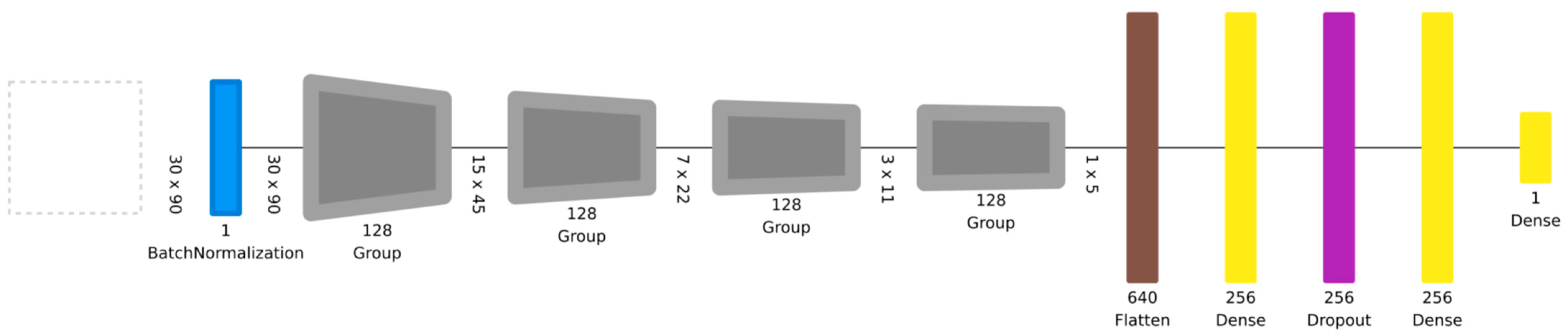
2022) on a data set containing approximately 150,000 observations. The network architecture is presented in
Figure 1. The model has four consecutive blocks (Group), each consisting of two convolutional layers (128 filters, size 3 × 3) with ReLU activations followed by a max-pooling layer (size 2). These blocks are followed by two fully connected (dense) layers (size = 256) and, finally, an output sigmoid classification layer (size = 1). The model architecture and hyperparameters (types of layers, number of layers, etc.) were decided on the basis of model performance on the validation data. See
Hjelkrem et al. (
2022) for further details on model architecture, hyperparameters, and model training.
4.2.2. A Wide and Deep Ensemble Model Using Open Banking Data and Handmade Features
Ensemble methods combine several learners to obtain better predictive performance than a single constituent learning algorithm. The ensemble method used in this paper is the XGBoost (eXtreme Gradient Boosting) boosting algorithm (
Chen and Guestrin 2016). The XGBoost algorithm has achieved excellent results in applied machine learning on structured tabular data. Gradient boosting is an ensemble technique in which new models are added to correct the errors made by existing models. The models are added sequentially until no further improvements can be made. This method is called gradient boosting because it uses a gradient descent algorithm to minimize the loss when adding new models. XGBoost is widely regarded as state-of-the-art among traditional machine learning methods in the realms of credit scoring, and we therefore do not consider other traditional machine learning or statistical methods in our experiments.
Figure 2 illustrates the Wide and Deep ensemble model. It uses the output from the first dense layer (256 deep learning features) of the already trained CNN model as explanatory variables for an XGBoost classifier. The output from the deep learning model can be viewed as automatically extracted features where the convolutional layers extract optimal representations from the raw data. In addition, the XGBoost algorithm are fed conventional, handmade features. Only hand-crafted features from external data sources are included, since internal data will not be available when scoring new customers.
The XGBoost classifier is trained on our training dataset with 6836 observations, and the hyperparameters are tuned using the validation dataset (864 obs.). The optimal hyperparameters are found using a Bayesian optimization framework called HyperOpt-Sklearn (
Bergstra et al. 2013;
Komer et al. 2014), and the optimal values for each parameter are presented in
Table 3.
4.3. Model Performance Evaluation
Model performance is evaluated by applying two commonly used metrics in credit risk modeling: Area Under the receiver operating characteristic Curve (AUC) and the Brier Score.
4.3.1. AUC
The receiver operating characteristic curve (ROC) is a two-dimensional graphical illustration of the trade-off between the true positive rate (sensitivity) and the false positive rate (1-specificity). The ROC curve illustrates the behavior of a classifier without having to take into account the class distribution or misclassification cost. The area under the receiver operating characteristic curve (AUC) is computed to compare the ROC curves of different classifiers. The AUC statistic is similar to the Gini coefficient, which is equal to 2 × AUC-1.
The AUC metric measures the discriminatory power of a classification model across a range of cut-off points (
Baesens et al. 2003). The AUC is particularly useful in practical terms, as banks may choose different cutoff points to manage risk tolerance. Furthermore, the AUC metric is not sensitive to class imbalance, as is commonly found in credit scoring.
4.3.2. Brier Score
The Brier score (
Brier 1950) measures how well calibrated the output predictions are. This metric is equivalent to the mean squared error but for a binary prediction task. A predicted output closer to the true label (Default/Non-default) produces a smaller error. Although a model should produce well-calibrated scores, in practice, it is not a requirement for a good classifier, as the probability cutoff point can be adjusted accordingly. Thus, we consider the Brier score a secondary metric to the AUC when evaluating model performance.
5. Experiments and Results
We examine the performance of our deep learning models on both a small and a large test dataset. In addition, we compare the performance of the deep learning models with the bank’s current application score models on the large test dataset. The main results of our experiments are summarized in
Table 4 and
Table 5 and
Figure 3.
Table 4 displays the performance results on the small test data set for our two deep learning models. Our deep learning model developed solely on Open Banking data (CNN) achieves an AUC of 0.835 on the small test set, while the wide and deep ensemble model (XGBoost) achieves an AUC of 0.899. The AUC performance gap can be attributed to the fact that the ensemble model has been developed on a richer dataset, i.e., both handmade features from external data (bureau data, tax statements, etc.) and Open Banking data (transactions).
In addition to the AUC, we also review how well calibrated the model predictions are using the Brier score metric. We find that the deep learning model (CNN) is poorly calibrated for the small test sample (Brier score = 0.139), while the wide and deep ensemble model (XGBoost) is better calibrated (Brier score = 0.052).
Since the small test dataset only contains 841 observations, we obtained a larger, more representative test sample as the basis for a review of the performance of the deep learning models as such and as a basis for comparison with the regression-based application models currently in use by the bank.
Table 5 presents the performance results on the large test dataset for our deep learning models and the bank’s current application models, while
Figure 3 illustrates the ROC curves underlying the AUC scores. We find that our two deep learning models perform better on the large dataset than on the small dataset. This is probably due to the difference in default rates in the two datasets. In addition, we find that the difference in performance between the two deep learning models is smaller for the large test data set than for the small data set. This indicates that the external data (bureau data, tax statements, etc.) contribute less to model performance on the larger, more representative dataset.
The deep learning model based solely on transaction data (CNN) achieves a surprisingly good AUC (0.91), outperforming the bank’s current application model for new customers (0.791). This indicates that the bank transactions from the last three months before the score date available through open APIs are considerably more predictive than the external data sources (bureau data, tax statements, etc.).
The wide and deep ensemble model employing Open Banking data (transactions) and handmade features (external data), is even better than the deep learning model, producing an AUC of 0.928.
As expected, the application model for existing customers outperforms our deep learning models as the model for existing customers is developed based on a richer information source (e.g., behavioral data from the last 1–2 years). Nevertheless, the performance gap between the application model for existing customers and the wide- and deep-ensemble model (XGBoost) is considerably smaller than the gap between the bank’s current application models for existing and new customers. This indicates that deep learning models applied to behavioral information in transactions from the last three months available through Open Banking APIs are capable of producing satisfactory default predictions for new customers. The discriminatory power is almost as good as that of the bank’s application model for existing customers. This is a very encouraging result, since the poor performance of existing credit default models with respect to assessing new customers, is a key problem in commercial banking. This important result bodes well for future practical applications of deep learning models in the banking industry.
Figure 4 illustrates the correlation between the predictions from the deep learning model based solely on Open Banking data (Prediction CNN) and the explanatory variables used by the bank’s current application model for existing customers using a correlation heatmap. Predictions from the Open Banking based model are mostly correlated to the banks explanatory variables containing information about the customers past financial behavior (Past financial behavior v1–v3). This is an unsurprising result since the bank’s explanatory variables for past financial behavior are also ultimately based on, among other things, aggregated, raw transaction data but typically include a broader observation window (up to 1–2 years).
In addition to the AUC, we also review how well-calibrated the model predictions are using the Brier score metric. We find that the deep learning model (CNN) is poorly calibrated for the small test sample (Brier score = 0.1264), while the wide and deep ensemble model (XGBoost) is better calibrated than the CNN model (Brier score = 0.0093). The bank’s application models currently in use for both existing and new customers are even better calibrated than the ensemble model (Brier score = 0.0032 and 0.0033, respectively).
6. Discussion and Conclusions
We find that the deep learning model for new customers based solely on Open Banking data (CNN) is surprisingly predictive of future loan defaults. It provides a significant improvement in discriminatory power compared to the conventional logistic regression credit scoring model for new customers based on traditional, handmade features from external data sources. This is probably mainly due to the fact that Open Banking data contains recent financial behavioral data (from the last 90 days), while traditional, handmade features from external data sources are based on older data (typically 1–2 years old). In addition, deep learning methods are able to automatically extract features from the Open Banking data that are superior to handmade features created by experts and can, to a higher degree, handle highly correlated features.
Furthermore, we find that the wide and deep ensemble model (XGBoost) based on both Open Banking data and traditional, handmade features from external data sources provides a minor lift in discriminatory power compared to the deep learning model based solely on Open Banking data (CNN). This result indicates that Open Banking data contains more predictive power than external data traditionally used in application credit scoring models for new customers (credit bureau data, tax statements, etc.). We find that the wide and deep ensemble model (XGBoost) has higher accuracy than the deep learning model based solely on Open Banking data (CNN). This is most likely due to the fact that the deep learning model (CNN) is trained on a dataset with less representative (higher) default rates than the wide and deep ensemble model (XGBoost). However, in practice, poor accuracy can be overcome by adjusting the cut-off score. Finally, we find that the conventional credit scoring model for existing customers is the best-performing credit scoring model. This is not surprising since this model is developed based on a dataset containing financial behavior data from the last 1–2 years. In contrast, Open Banking APIs only provide access to financial behavior data from the last 90 days.
Our results also suggest that data available through the Open Banking APIs is highly useful for banks assessing the creditworthiness of potential new customers. In combination with deep learning and ensemble methods, such data may have the potential to substantially increase the performance of banks’ application credit scoring models and thus increase the profitability of banks when recruiting new customers.
Furthermore, our results indicate that banks have an advantage over Fintechs and other financial intermediates without access to historical data on customers’ transactions and balances in developing the best application credit scoring models for new customers. In addition, our results suggest that using Open Banking data in application credit scoring models might reduce the need for traditional, external data sources (bureau data, tax statements, etc.) when developing models and scoring potential customers.
Finally, we believe that including Open Banking data in application score models will lay the foundation for streamlining the application process, which in turn will be able to free up resources in banks and improve the customer experience when potential customers apply for loans.
Limitations and Further Research
This study is based solely on data from a Norwegian bank’s current customers. The results in this study are therefore not necessarily fully transferable to the assessment of actual applications from new customers, and future research should focus on developing credit scoring models on data from actual application cases where Open Banking data are obtained as a part of the application assessment process.
Furthermore, research on prediction explainability for deep learning models is necessary since current regulations demand that banks can explain rejections of applications from customers. In addition, this analysis could be expanded by including textual descriptions and categories of the transactions to examine whether this would further increase the models’ performance.


