Article

An Empirical Study of Volatility in Cryptocurrency Market

Department of Finance, Jaipuria Institute of Management, Lucknow 226010, India
*
Author to whom correspondence should be addressed.
J. Risk Financial Manag. 2022, 15(11), 513; https://doi.org/10.3390/jrfm15110513
Submission received: 4 October 2022 / Revised: 31 October 2022 / Accepted: 2 November 2022 / Published: 4 November 2022

Abstract

:
Cryptocurrencies have gained a lot of attraction across the globe. Most observers of the cryptocurrency market will agree that crypto volatility is in a different league altogether. There has been a growing need to understand the nature of volatility in cryptocurrency. This paper analyzes the performance of four mostly traded, different cryptocurrencies in terms of their risk and return. The relationship between the return and returns volatility among different currencies has been examined considering the daily closing prices from 1 January 2017 to 30 June 2022, using the family of the GARCH model. The study has explored the spillover and asymmetric effect of volatility by using the DCC GARCH model and EGARCH model, respectively. The causal behavior among different cryptocurrencies has also been examined using Granger causality. There has been a strong spillover effect among different cryptocurrencies, Bitcoin and Ether, which are the top two cryptocurrencies with the highest market capitalization which have exhibited an asymmetric impact in their volatility as compared to the other two currencies, which are Litecoin and XRP.

1. Introduction

In recent times, cryptocurrencies are gaining a lot of popularity as they create more opportunities for worldwide business and they mitigate risk. This attraction has been accentuated by its decentralized nature. There were more than 18,000 currencies across the globe by March 2022, even though many of them are thinly traded. The total market cap of all cryptocurrencies which are trading is touching more than USD 1.5 trillion, as of June 2022 (https://coinmarketcap.com/coins/, accessed on 10 July 2022). An exponential growth has been witnessed over the last few years. It is in this context which it is important to analyze the behavior of the crypto market and its ecosystem in. Out of many, the four most traded cryptocurrencies are Bitcoin, Ether, Litecoin, and Ripple (XRP). Bitcoin, the oldest among all the cryptocurrencies, is a decentralized digital currency without any central bank as a controller. It is increasingly becoming accepted by merchants and retailers for making payments. Miners in the Bitcoin network make money by validating blocks (Schilling and Uhlig 2019). The Ethereum platform is the second largest blockchain platform; this provides an opportunity to deploy immutable applications on it. The platform gains attraction as this technology can facilitate online payments, loan distribution, and commodity training, thus increasing the demand for Ether (ETH), the cryptocurrency used to transact on the Ethereum platform. Ether is used to pay for transaction fees and computational services. The process of mining helps Ether come into existence by the validation of transactions on the Ethereum platform. Ether has a good demand and is used as a launch platform for all kinds of decentralized applications, ranging from DeFi (decentralized finance) to games and even to NFTs. Litecoin is a cryptocurrency designed for peer-to-peer transactions and has a better transaction speed than bitcoin. The primary objective of Litcoin was to mirror the performance of Bitcoin by scaling up the volume, which will allow for transactions of small payments. Even though, to a certain extent, the goal has been achieved, there are still new blockchain innovations that are coming into the crypto market. XRP, the token created by the US Company Ripple, is also an altcoin like Litecoin and is a coin that banks use to transfer value over borders quickly and easily. The Ripple System has lower processing times and lower transaction charges.
In financial markets, volatility refers to a deviation in the price of an asset. Healthy volatility creates opportunities for profit. Crypto or digital currencies seem to be the future of money. Crypto is a high-risk and high-return investment asset class. The estimation of the volatility of return enables us to assess the possibility of specific outcomes. There have been several studies to investigate the nature of volatility in assets. With the rise in the popularity of cryptocurrency, there has been an emphasis on analyzing the volatility of cryptocurrencies and comparing it with other financial assets. Ciaian et al. (2016) observed that receiving a return in Bitcoin is not influenced by macro financial factors. Corbet et al. (2018) identified that cryptocurrencies can be used for hedging and they do provide diversification benefits to investors. Shahzad et al. (2019) identified Bitcoin, along with gold and the commodity index, as assets which can act as a weak hedge in some cases. Some of the key issues to analyze are the interrelationship among different cryptocurrencies and also the asymmetric volatility phenomenon in the crypto market.
There are various methods to assess volatility wherein time-varying volatility models hold an importance in the literature (Rastogi 2014). The characteristics in volatility play an important role in the development of various models. The GARCH group of models has been reliably displayed to yield the most dependable outcomes, and hence, the GARCH framework has turned into the standard technique for demonstrating the unpredictability in financial time series data (Brooks et al. 2002). In financial data, we observe asymmetric behavior in the volatility, also referred to as the leverage effect. For instance, in the equity market, the conditional volatility in equity markets is more affected by the presence of negative news than positive news. Horpestad et al. (2019) have explored the asymmetric behavior of nineteen global indices across the globe. It will be interesting to investigate whether similar behavior is depicted by cryptocurrencies also. Chu et al. (2017) have examined the volatility of seven different cryptocurrencies by different GARCH models and concluded EGARCH to be a suitable fit for explaining the asymmetric nature of volatility. It is generally believed in theories of finance that the return generated by any assets can be explained by the risk associated with it and therefore Engle et al. (1987) first proposed a model called the GARCH in mean (GARCH-M) model where a heteroscedasticity term is added to the conditional mean function. While analyzing multiple time series, it becomes imperative to identify the impact of one time series over another. It is in this context that Multivariate GARCH models often help in estimating the time-varying correlations among different series. The multivariate model called the dynamic conditional correlation (DCC) model developed by Engle (2001) performs well and provides sensible and accurate results. It also helps in understanding the volatility spillover of one currency over other.
There have been two schools of thought in understanding the interrelationship and volatility spillover among cryptocurrencies. First, it has been observed that the crypto market has depicted the characteristics of an efficient market in which Stavroyiannis (2018), Baur and Dimpfl (2018) have identified the leverage effect in Bitcoin. Dutta and Bouri (2022) identified that there exists a significant presence of time varying jumps in Bitcoin. The other school of thought states that crypto markets are inefficient. Fry and Cheah (2016) have examined the bubbles created in the crypto market and considered the market to include speculative components and to be highly volatile.
By identifying the interrelationships among different cryptocurrencies and measuring their volatility of returns, the market participants such as miners and investors will be able to make an informed decision. There has been a significant growth in the cryptocurrency market but there is not enough empirical evidence to suggest any diversification and hedging properties among the different cryptocurrencies. Bouri et al. (2021) observed in cryptocurrencies a return connectedness increases with both kind of shocks, implying an increase in the volatility during extreme events.
Based on these contexts, the present study contributes to examining the behavior of four major cryptocurrencies. The study examines the causality relationship among cryptocurrencies and also the nature of volatility in different cryptocurrencies and its spillover effect over each other. The impact of asymmetric information on the different cryptocurrencies is also examined.
The rest of the paper is organized as follows. Section 2 discusses the source of data and its transformation for the study. It presents the descriptive statistics, the correlation, and a graphical presentation for exploring the performance. In Section 3, we have discussed the analysis of the data by using the Granger causality test to check the causality between the different coins over each other. The univariate GARCH, EGARCH, GARCH-M, and multivariate DCC GARCH models have been applied to understand the volatility behavior of the four mostly traded cryptocurrencies. In Section 4, the discussion and conclusion have been made for policy implications.

2. Data

Descriptive Statistics

In the study, we have examined four cryptocurrencies Bitcoin, Ether, Litecoin, and XRP. Even though there are more than eighteen thousand cryptocurrencies in the market, most of them are very thinly traded and are very nascent in the market. These four currencies have the highest market capitalization (Table 1) as of 30 June 2022 and they have been in the market for more than five years. The data in the study were taken from 1 January 2017 to 30 June 2022 and consists of the daily closing price of the currencies in USD, taken from the website of CoinMarketCap (https://coinmarketcap.com/coins/, accessed on 10 July 2022). The daily log returns are calculated by using the formula below:
R i t = ln ( P i t P i , t 1 )
  • Rit = Daily log return of cryptocurrency at day t;
  • Pit = Closing price of crypto at day t;
  • Pi,t−1 = Closing price of crypto at day t − 1.
In Table 2, the descriptive statistics of daily closing returns of all the cryptocurrencies in the study are reported. As observed in Table 2, Ether had the highest daily average return (0.32%), however, Bitcoin had the highest median daily return (0.23%). It has also been observed that there was a negative skewness in Bitcoin and Ether, which have the highest market capitalization, whereas XRP and Litecoin showed a positive skewness. Even the kurtosis of all the currencies is on the higher side, forming a leptokurtic distribution, which indicates that the log returns of all the currencies in the study are more centered around the mean compared to the normal distribution. The J-B Statistics (Jerque-Bera) and corresponding p-values confirm that the return data of these cryptocurrencies are not normal at a 1% significance level. The clustering nature of the returns is also observed in Figure 1.
There is also the presence of a high positive correlation in Table 3 among all the cryptocurrencies, however, the correlation is high between Ether and Bitcoin (0.712) compared to the other pairs, indicating that the two currencies have the highest market capitalization and that they have a strong relationship.
The holding period performance of these currencies has been explored in Table 4. The rolling returns for one year, three years, and five years are seen to investigate the returns generated for investing in the long term. Even though there has been a phenomenal return generated over five years by all currencies, it is accompanied by a very high volatility.

3. Data Analysis

The pre-requisite for the application of GARCH modeling is to check for the stationarity of data and for the presence of heteroscedasticity for the residuals. The presence of heteroscedasticity explains the need for the GARCH framework for modeling the conditional volatility.

3.1. Unit Root Test

It is necessary to have stationary data or else it will yield spurious regression results. If the series is non-stationary, then its distribution will change in every period and hence it will be difficult to establish a relationship or do any forecasting. If the series is stationary, it implies that in the time series the data structure is stable, which implies a constant mean, variance, and covariance over time.
To check for the unit root problem, the augmented Dickey–Fuller (ADF) test was applied (Dickey and Fuller 1981) in which the null hypothesis of the test is that the data are not stationary.
y t = 0 + θ y t 1 + i = 1 n y t + e t ,
In the above, ‘ y t ’ indicates the data in time t, ‘n’ is the optimum number of lags, αo is the constant, and ‘e’ is an error term.
In the data set, it has been observed (Table 5) that all the cryptocurrency returns are exhibiting stationarity.

3.2. ARCH Effect Test

The presence of heteroscedasticity for residuals is tested by applying the ARCH-LM test (autoregressive conditional heteroscedasticity–Lagrange multiplier test) (Ljung and Box 1978)
u t 2 = γ 0 + γ 1 u t 1 2 + γ 2 u t 2 2 + + γ p u t p 2 + v t ,
u represents the square residual of the Mean regression model and p indicates the lag length in the residual regression model.
The null hypothesis of the ARCH–LM test is that the coefficients of the squared residuals in Equation (3) are insignificant which means γ 0 = γ 1 = γ 2 = γ p = 0 , thus there is no heteroscedasticity in the time series data or there is no ARCH effect present in data.
As observed in Table 6, the ARCH effect is prevalent in returns of the cryptocurrency and thus it is imperative to apply the GARCH model to identify the impact of the conditional volatility.

3.3. Granger Causality

The Granger causality test has been applied to explore any relationship in the returns among the different cryptocurrencies. We have used the following equation to test for the Granger causality relationship:
y t = a 0 + a 1 y t 1 + a 2 y t 2 + a p y t p + b 1 x t 1 + b 2 x t 2 + b p x t p + t
x t = c 0 + c 1 x t 1 + c 2 x t 2 + c p x t p + d 1 y t 1 + d 2 y t 2 + d p y t p + t
The null hypothesis in Equation (4) in series X does not Granger cause Y, implying that all the coefficients of x are zero. If any coefficient of X is significantly different from zero, it will be concluded that series X is influencing the returns of series Y. Similarly in Equation (5), the null hypothesis is Series Y does not Granger cause X, which will be true if all the coefficients of y are zero.
As observed in Table 7, there exists an unidirectional causality between Bitcoin and Ether where Ether is influencing the return in Bitcoin. A similar univariate relationship has been observed between XRP and bitcoin, and also between XRP and Ether.
Estimating mean equation: we have adopted the ARIMA (1,1) model (autoregressive moving average model) as the best fit model to identify the impact of the past return and residual in the return of cryptocurrencies.
Conditional Mean Equation:
y t = c + b 1 y t 1 + b 2 e t 1 + e t ,
y t is the conditional mean, c is the intercept, b 1 is the coefficient of AR (1), b 2 is the coefficient of MA (1), and e t indicates the error at time t.
As seen in Table 8, we observe that Bitcoin, Ether, and Litecoin are getting influenced by the past returns and also the residuals.

3.4. GARCH Model

The volatility in the time series data is captured by the Generalized ARCH (GARCH) model (Bollerslev 1986) which is an extension of the ARCH model. These models capture the effect of the news on the volatility of data and also the persistency of the volatility in the data. The GARCH (1,1) model incorporating the effect of the news and volatility of the last day can be expressed as follows (Brooks and Rew 2002):
Conditional variance equation (GARCH (1,1)
h t 2 = ω + α 1 ε t 1 2 + β 1 h t 1 2
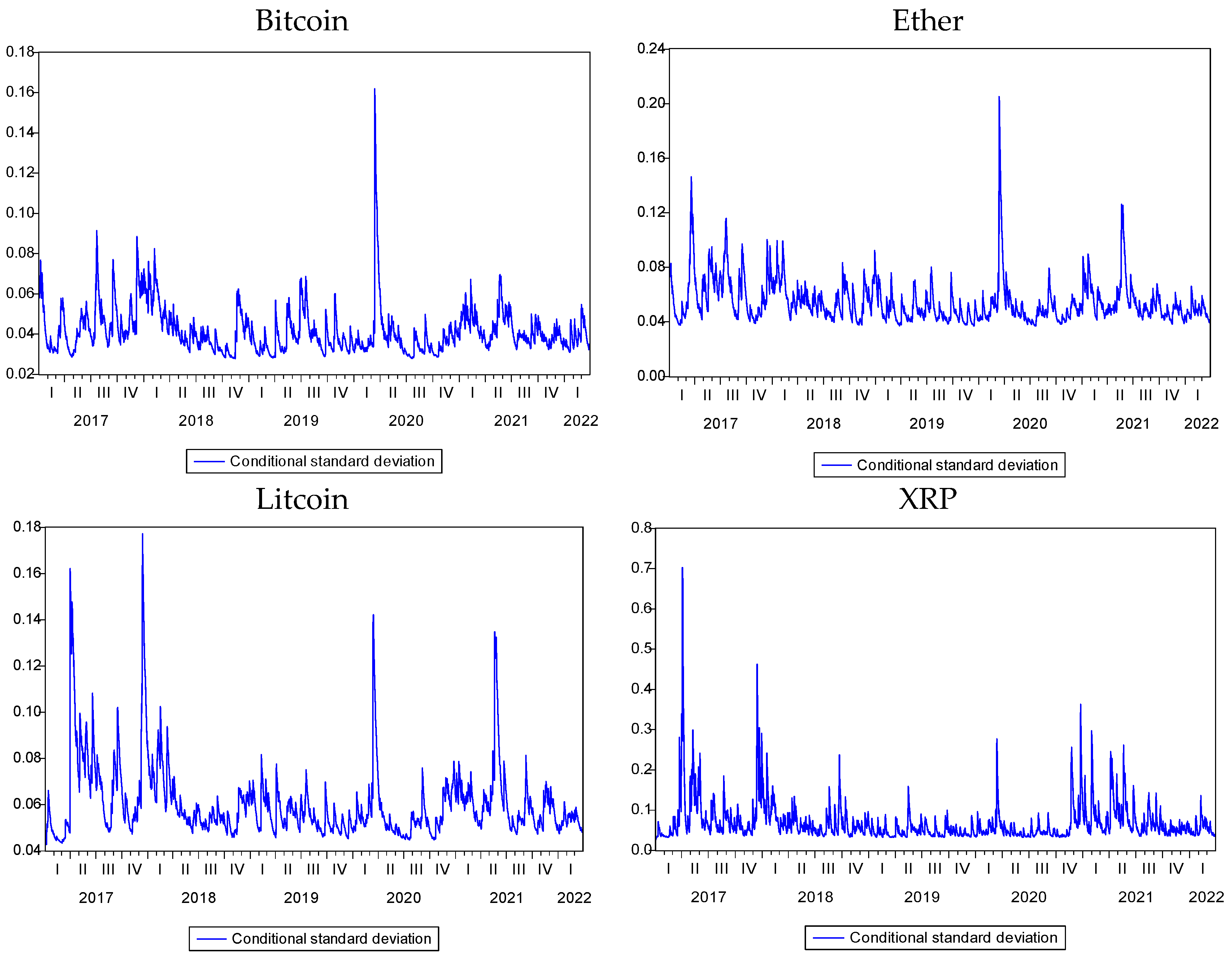
In the above Equation (7), α1 and β1 are coefficients of the ARCH and GARCH terms, respectively, where ‘ α 1 ’ represents the ARCH effect which estimates the response to any shock or news in the crypto currency market. ‘ β 1 ’ represents the GARCH effect which identifies the persistency of the volatility. A high ARCH coefficient ( α 1 ) indicates a greater sensitivity of volatility to the news coming and a high GARCH ( β 1 ) value depicts the presence of a high persistency of volatility and the volatility taking more time to die out (Chaudhary et al. 2020; Rastogi 2014). The GARCH model will be stable only if the sum of α 1 and β 1 will be less than one or else the data will reflect an explosive nature. As seen in Table 9, there is a strong presence of the ARCH and GARCH effects across all the cryptos and there is a strong persistency factor across all the cryptos. A high volatility across all currencies can be observed from the GARCH graphs (Figure 2).

3.5. EGARCH Model

The asymmetric behavior of the volatility in cryptocurrencies is investigated by using the E-GARCH (exponential GARCH) model by Nelson (1991). The E-GARCH model captures the impact of low and high volatility regimes in cryptocurrencies. The model is widely used to capture the leverage effect of shocks on different financial markets. Baur (2012), Christie (1982), Gupta et al. (2022), and Campbell and Hentschel (1992) have observed that negative news brings more volatility as compared to positive news. This behavior in financial markets is primarily because of the leverage effect of firms on volatility.
ln ( h t ) = α 0 + α 1 u t 1 h t 1 + λ u t 1 h t 1 + β ln ( h t 1 )
The log of variance of the cryptocurrency return data ( h t ) makes the leverage effect exponential rather than quadratic. This modification ensures that the estimates are non-negative. In Equation (8), α 1 indicates the coefficient of the ARCH effect, which models the impact of past news and also incorporates the size effect of the news, and λ represents the coefficient identifying the presence of the asymmetric effect, also referred to as the sign effect of the news. If λ < 0, it implies that bad news (negative shocks) in the cryptocurrency markets generates a larger volatility than any good news (positive shocks) and β represents the coefficient of the GARCH term, which shows the persistency of the volatility.
As seen in Table 10, there is a significant effect of asymmetry across Bitcoin, Ether, and Litecoin. As with the presence of negative news, the volatility tends to increase in Bitcoin and Ether, whereas in Litecoin and XRP, it tends to fall.

3.6. GARCH in Mean (GARCH-M) Model

Investors who are averse to risk seek a premium before choosing an asset for their investment. The return derived from any asset has to be a function of the risk associated with it, as postulated in the capital asset pricing model (Sharpe 1963). The same conditional mean function is modified by incorporating the conditional variance as an explanatory variable.
In the GARCH-M, model the conditional mean is explained by its conditional variance, allowing the conditional mean to depend on its conditional variance.
y t = δ h t 1 + c + α y t 1 + β e t 1
In Equation (9) above, yt which is the return of the cryptocurrency, is taken as a function of its past volatility ( h t 1 ) and if the coefficient of h t 1 denoted as δ is significant and also positive, then it can be concluded that the increase in the risk is compensated by high returns and δ can be attributed to the risk premium.
We can infer that the mean return of the cryptocurrencies increases because of the higher presence of volatility if parameter δ in Equation (9) is positive and significant However, if δ is insignificant, it can be concluded that the return of the cryptocurrencies is not influenced by the past volatility.
As observed in Table 11, the relationship between the volatility and the return does not exist in all cryptos.

3.7. DCC(1,1) Model

We have adopted the GARCH model with the dynamic conditional correlation (DCC), formulated by Engle (2001). The model adopts correlation impact along with the GARCH model. It models the dynamic process of the volatile conditions and their dependencies. These models not only model the variance and covariance, but they also predict the flexibility of variance (Yan et al. 2022). The current values in the DCC GARCH model are related to their past values and square residuals.
Assuming two-time series data sets, ri,t and rj,t, and then deploying the AR(1) models, there are two residual time variables, ai,t and aj,t. For these two variables, Ht represents the dynamic conditional covariance matrix of two-time series ri,t and rj,t.
Rt:
represents the dynamic conditional correlation (DCC) matrix.
Dt:
represents the diagonal matrix from the covariance matrix Ht.
Dt−1:
the inverse of the Dt Matrix.
Then, the relationship between the matrices of Ht, Rt, Dt, and Dt−1 is:
Ht = DtRtDt
Rt = Dt−1HtDt−1
After adopting two GARCH (1,1) models, we obtained two normalized residual variables εi,t and εj,t; the following relationship is obtained by defining the following variables
Qt 
indicates Covariance Matrix
Gt 
indicates the diagonal matrix of the covariance matrix Qt,
Qt−1 
indicates the inverse matrix of the matrix Qt.
Ct 
indicates Correlation Matrix
The relationships between the matrices of Qt, Ct, Gt, and Dt−1 are:
Qt = GtCtGt
Ct = Gt−1 QtGt−1
For a two-order matrix, Rt, Ht, and Qt, assume:
R t = ρ i , t ρ i j , t ρ j i , ρ j , t , H t = [ σ i , t σ i j , t σ j i , t σ j , t ] Q t = [ q i , t q i j , t q j i , t q j , t ]
σij,t = σi,tρij,tσj,t,  σji,t = σi,tρji,tσj,t
Using the relationships of ai,t = σi,tεi,t and aj,t = σj,tεj,t from AR(1) and GARCH(1,1) (Engle 1982, 2001).
The dynamic conditional correlations between the two series can be defined as:
ρ i j , t = q i j , t q i , t q j , t , ρ j i , t = q j i , t q j , t q i , t   where ρ i j , t = ρ j i , t
Because the time variable t is considered, the correlation variables ρij,t and ρji,t are the varying correlation.
The dynamic correlation process is driven by two parameters (α) and (β). Both the estimators which are obtained from the DCC GARCH model are dynamic and vary with time. The α coefficient in the DCC model measures the short-run volatility impact in cryptocurrencies, which indicates the persistency of the standardized residuals from the previous period.
The β coefficient in the DCC model measures the lingering effect of the shock impact on the conditional correlations. The sum of these two parameters is less than one, which indicates that the conditional correlation in the models is not constant over time and the model is stable.
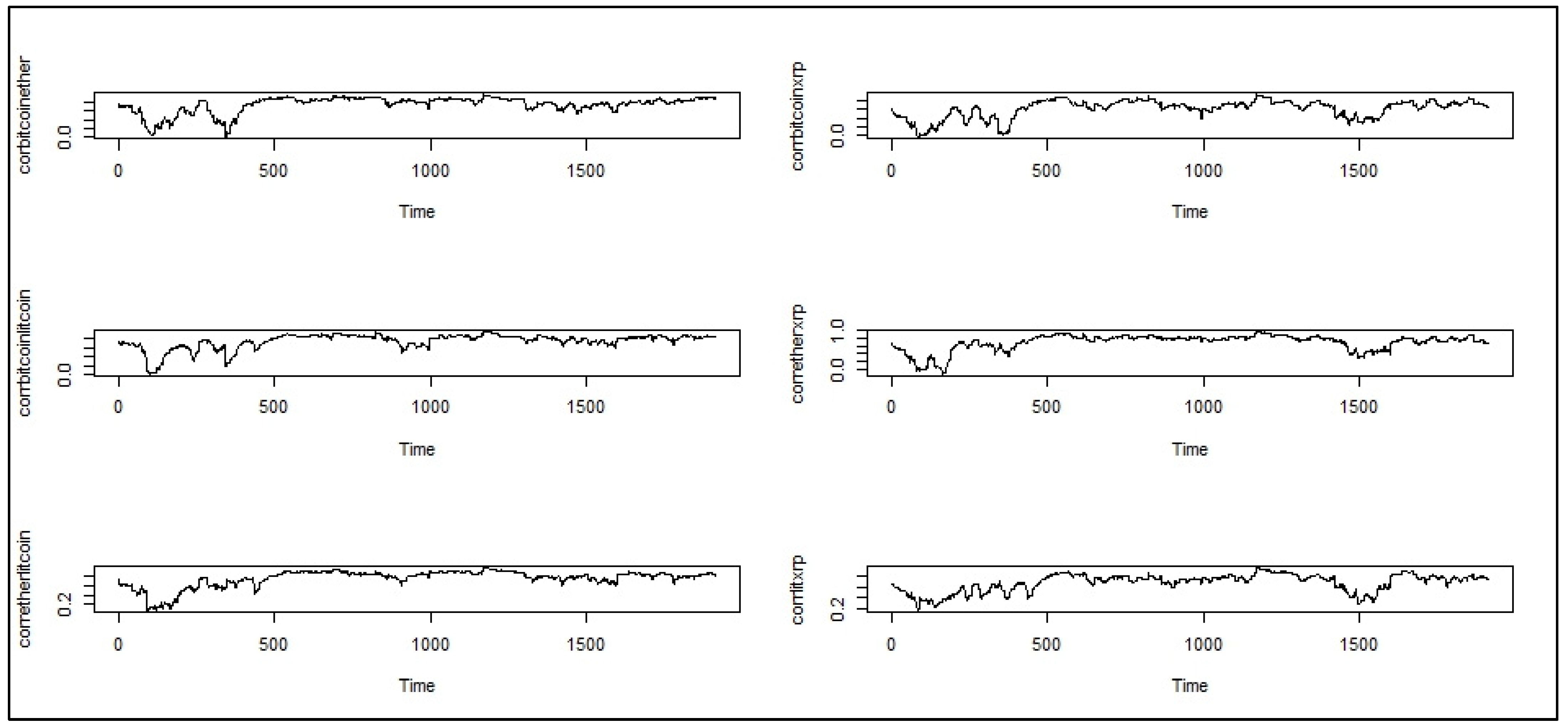
Similar results can also be observed from the DCC graphs (Figure 3) over the period as a similar trend in the correlations is observed across all the cryptocurrencies. By analyzing the mean of the dynamic correlation over the period (Table 12), a strong correlation among all the currencies was observed even though, relatively XRP, showed a low correlation with other currencies.
As seen in Table 13, it is observed that there exists a spillover effect for both the short-term and long-term across all the currencies and also across all the pairs of currencies. This indicates the strong interrelationship in the volatility among the different currencies. The β coefficient of all the pairs in the DCC model is more than 0.9, which indicates the presence of a very strong lingering effect of the shock impact on the conditional correlations across all the pairs of currencies. There was also the existence of persistency of volatility over some time. Abakah et al. 2020 also observed similar results and also concluded that this persistent behavior is reduced if the structural breaks are incorporated.

4. Discussion and Conclusions

The main feature of any cryptocurrencies which are based on the blockchain concept is their decentralized character and how they are free from any control and intervention. These characteristics make it a preferred medium of exchange, and also an investment. The opportunity given in cryptocurrency trading is something new and is challenging to match in the customary field.
This study focuses on identifying the nature of the volatility and interdependence of the different cryptocurrencies. It has been observed that there is a presence of a high volatility among the returns of these cryptocurrencies, and hence these are very risky assets for investments. We do not observe a very strong bivariate causal relationship among the currencies and only a univariate relationship of Ether and XRP influencing the Bitcoin returns and XRP influencing the Ether returns were observed. Even though in the last few years these currencies have given excellent returns (Table 4), there has been a very high volatility. It has also been observed that Bitcoin and Ether, having the highest market capitalization, exhibit a different behavior compared to the other currencies, which are Litecoin and XRP. This is in contrast to the finding by Qiang Ji et al. (2019) which revealed that the return and volatility is not related to market capitalization as, from the observations of GARCH(1,1) models, the beta coefficient in the model was higher, that is, more than 0.6 for all the currencies, implying the presence of high volatility clustering and a memory persistence in the long run. Similar results were also observed by Kaya Soylu et al. (2020), Abakah et al. (2020), and Sensoy et al. (2021). Bitcoin and Ether both have exhibited an asymmetric impact in their volatility and with the presence of negative news, this volatility tends to increase. This behavior is similar to the behavior shown by stock markets where the volatility tends to increase with negative news (Gupta et al. 2022). However, in the other two currencies, Litcoin and XRP, the presence of negative news tends to reduce the volatility. This characteristic displayed by Litcoin and XRP resonates with the investment in gold (Baur 2012), and thus these two currencies can act as better hedgers compared to Bitcoin and Ether. Shahzad et al. (2020) in his study also found that gold is a better asset for hedging than Bitcoin. This phenomenon can be attributed to the fact that the market cap of Bitcoin and Ether is on the higher side; where the demand for Bitcoin and Ether is high, which can be attributed to their usage, Bitcoin has been finding an acceptability, such as in El Salvador, because it has become the first country in the world to accept Bitcoin as a legal tender. The demand for Ether is growing because of the high demand for decentralized open-source applications in the Ethereum platform. An upgrade of Ethereum’s algorithm that will transition it from proof of work to proof of stake is also a sign of Ether performing well. A similar attraction has not been seen in XRP and Litecoin. Litecoin, which was created as a parallel to Bitcoin to reduce the processing time, has failed to get the desired volume. XRP being used preferably by banking and financial services companies for faster payments seems to have the lesser attraction from individuals. The findings reflect that market capitalization is influencing the asymmetric nature of the volatility of cryptocurrencies. Similar findings were also observed by Phillip et al. (2018), that cryptos of a relatively lower volume are more vulnerable to price speculation. It is seen that the volatility behavior of Bitcoin and Ether, which have a high market capitalization, tends to depict behavior closer to the stock markets. We could not find any relationship in the volatility explaining the return of these currencies, as seen by the GARCH-M model. This is in contrast to the theoretical premise that with an increased volatility, we can expect higher returns. There does exist a strong spillover effect across all the currencies and they also exhibited a strong dynamic correlation over some time. The findings are similar to Yan et al. (2022), Ciaian et al. (2018), and Lahajnar and Rozanec (2020). The volatility impact is persisting for the long term, as observed in Table 13, where we have seen that the beta (β) coefficient in the DCC model is significantly higher than the alpha (α) coefficients. This also indicates the persistence of the conditional correlation process across all the pairs of currencies.
The findings of the study will enable fund managers and investors to take more informed decisions while evaluating their investment decisions in cryptocurrencies. This will also help them in understanding the usage of cryptocurrency as a hedging alternative in designing an investment portfolio as the study has revealed that the risk–return relationship applicable in other investment options is not depicted in any of these currencies. We also observed a strong spillover effect of the volatility across the different cryptocurrencies. This spillover effect and different behavior of cryptos towards the asymmetric volatility can assist crypto traders in creating hedging strategies for managing risk. The study was conducted on four prominent cryptos, out of more than eighteen thousand cryptos which are prevailing, and thus it will be interesting to explore in future studies the nature of the risk and return behavior of other cryptos and their future and acceptability across the globe.

Author Contributions

Conceptualization, H.G. and R.C.; methodology, H.G. and R.C.; software, HG.; validation, H.G. and R.C.; formal analy-sis, H.G. and R.C.; investigation, H.G. and R.C.; resources, H.G. and R.C.; data curation, H.G.; writing—original draft preparation, H.G.; writing—review and editing, H.G. and R.C.; visualization, H.G. and R.C.; supervision, H.G. and R.C.; project administration, H.G and R.C. All authors have read and agreed to the published version of the manuscript.

Funding

This research received no external funding.

Data Availability Statement

Not applicable.

Conflicts of Interest

The authors declare no conflict of interest.

References

  1. Abakah, Emmanuel Joel Aikins, Luis Alberiko Gil-Alana, Godfrey Madigu, and Fatima Romero-Rojo. 2020. Volatility persistence in cryptocurrency markets under structural breaks. International Review of Economics & Finance 69: 680–91. [Google Scholar]
  2. Baur, Dirk G. 2012. Asymmetric volatility in the gold market. The Journal of Alternative Investments 14: 26–38. [Google Scholar] [CrossRef]
  3. Baur, Dirk G., and Thomas Dimpfl. 2018. Asymmetric volatility in cryptocurrencies. Economics Letters 173: 148–51. [Google Scholar] [CrossRef]
  4. Bollerslev, Tim. 1986. Generalized autoregressive conditional heteroskedasticity. Journal of Econometrics 31: 307–27. [Google Scholar] [CrossRef] [Green Version]
  5. Bouri, Elie, Tareq Saeed, Xuan Vinh Vo, and David Roubaud. 2021. Quantile connectedness in the cryptocurrency market. Journal of International Financial Markets, Institutions and Money 71: 101302. [Google Scholar] [CrossRef]
  6. Brooks, Chris, and Alistair G. Rew. 2002. Testing for a unit root in a process exhibiting a structural break in the presence of GARCH errors. Computational Economics 20: 157–76. [Google Scholar] [CrossRef]
  7. Brooks, Chris, Olan T. Henry, and Gita Persand Persand. 2002. The effect of asymmetries on optimal hedge ratios. The Journal of Business 75: 333–52. [Google Scholar] [CrossRef] [Green Version]
  8. Campbell, John Y., and Ludger Hentschel. 1992. No news is good news: An asymmetric model of changing volatility in stock returns. Journal of Financial Economics 31: 281–318. [Google Scholar] [CrossRef] [Green Version]
  9. Chaudhary, Rashmi, Priti Bakhshi, and Hemendra Gupta. 2020. Volatility in international stock markets: An empirical study during COVID-19. Journal of Risk and Financial Management 13: 208. [Google Scholar] [CrossRef]
  10. Christie, Andrew A. 1982. The stochastic behavior of common stock variances: Value, leverage and interest rate effects. Journal of Financial Economics 10: 407–32. [Google Scholar] [CrossRef]
  11. Chu, Jeffrey, Stephen Chan, Saralees Nadarajah, and Joerg Osterrieder. 2017. GARCH modelling of cryptocurrencies. Journal of Risk and Financial Management 10: 17. [Google Scholar] [CrossRef]
  12. Ciaian, Pavel, Miroslava Rajcaniova, and d’Artis Kancs. 2016. The economics of BitCoin price formation. Applied Economics 48: 1799–815. [Google Scholar] [CrossRef] [Green Version]
  13. Ciaian, Pavel, Miroslava Rajcaniova, and Artis Kancs. 2018. Virtual relationships: Short- and long-run evidence from BitCoin and altcoin markets. Journal of International Financial Markets, Institutions & Money 52: 173–95. [Google Scholar]
  14. Corbet, Shaen, Andrew Meegan, Charles Larkin, Brian Lucey, and Larisa Yarovaya. 2018. Exploring the dynamic relationships between cryptocurrencies and other financial assets. Economics Letters 165: 28–34. [Google Scholar] [CrossRef] [Green Version]
  15. Dickey, David A., and Wayne A. Fuller. 1981. Likelihood ratio statistics for autoregressive time series with a unit root. Econometrica: Journal of the Econometric Society 49: 1057–72. [Google Scholar] [CrossRef]
  16. Dutta, Anupam, and Elie Bouri. 2022. Outliers and Time-Varying Jumps in the Cryptocurrency Markets. Journal of Risk and Financial Management 15: 128. [Google Scholar] [CrossRef]
  17. Engle, Robert F. 1982. Autoregressive conditional heteroscedasticity with estimates of the variance of United Kingdom inflation. Econometrica: Journal of the Econometric Society 50: 987–1007. [Google Scholar] [CrossRef]
  18. Engle, Robert. 2001. GARCH 101: The use of ARCH/GARCH models in applied econometrics. Journal of Economic Perspectives 15: 157–68. [Google Scholar] [CrossRef] [Green Version]
  19. Engle, Robert F., David M. Lilien, and Russell P. Robins. 1987. Estimating time varying risk premia in the term structure: The ARCH-M model. Econometrica: Journal of the Econometric Society 55: 391–407. [Google Scholar] [CrossRef]
  20. Fry, John, and Eng-Tuck Cheah. 2016. Negative bubbles and shocks in cryptocurrency markets. International Review of Financial Analysis 47: 343–52. [Google Scholar] [CrossRef] [Green Version]
  21. Gupta, Hemendra, Rashmi Chaudhary, Kajal Srivastava, and Suneel Gupta. 2022. Volatility modelling of asset classes: An empirical study during different phases of COVID-19. Academy of Accounting and Financial Studies Journal 26: 1–19. [Google Scholar]
  22. Horpestad, Jone B., Štefan Lyócsa, Peter Molnár, and Torbjørn B. Olsen. 2019. Asymmetric volatility in equity markets around the world. The North American Journal of Economics and Finance 48: 540–54. [Google Scholar] [CrossRef]
  23. Ji, Qiang, Elie Bouri, Chi Keung Marco Lau, and David Roubaud. 2019. Dynamic connectedness and integration in cryptocurrency markets. International Review of Financial Analysis 63: 257–72. [Google Scholar] [CrossRef]
  24. Kaya Soylu, Pınar, Mustafa Okur, Özgür Çatıkkaş, and Z. Ayca Altintig. 2020. Long memory in the volatility of selected cryptocurrencies: Bitcoin, Ethereum and Ripple. Journal of Risk and Financial Management 13: 107. [Google Scholar] [CrossRef]
  25. Lahajnar, Sebastian, and Alenka Rozanec. 2020. The correlation strength of the most important cryptocurrencies in the bull and bear market. Investment Management and Financial Innovations 17: 67–81. [Google Scholar] [CrossRef]
  26. Ljung, G.M., and G. E. Box. 1978. On a measure of lack of fit in time series models. Biometrika 65: 297–303. [Google Scholar] [CrossRef]
  27. Nelson, Daniel B. 1991. Conditional heteroskedasticity in asset returns: A new approach. Econometrica: Journal of the Econometric Society 59: 347–70. [Google Scholar] [CrossRef]
  28. Phillip, Andrew, Jennifer S. K. Chan, and Shelton Peiris Peiris. 2018. A new look at cryptocurrencies. Economics Letters 163: 6–9. [Google Scholar] [CrossRef]
  29. Rastogi, Shailesh. 2014. The financial crisis of 2008 and stock market volatility–analysis and impact on emerging economies pre and post crisis. Afro-Asian Journal of Finance and Accounting 4: 443–59. [Google Scholar] [CrossRef]
  30. Schilling, Linda, and Harald Uhlig. 2019. Some simple bitcoin economics. Journal of Monetary Economics 106: 16–26. [Google Scholar] [CrossRef]
  31. Sensoy, Ahmet, Thiago Christiano Silva, Shaen Corbet, and Benjamin Miranda Tabak. 2021. High-frequency return and volatility spillovers among cryptocurrencies. Applied Economics 53: 4310–28. [Google Scholar] [CrossRef]
  32. Shahzad, Syed Jawad Hussain, Elie Bouri, David Roubaud, Ladislav Kristoufek, and Brian Lucey. 2019. Is Bitcoin a better safe-haven investment than gold and commodities? International Review of Financial Analysis 63: 322–30. [Google Scholar] [CrossRef]
  33. Shahzad, Syed Jawad Hussain, Elie Bouri, David Roubaud, and Ladislav Kristoufek. 2020. Safe haven, hedge and diversification for G7 stock markets: Gold versus bitcoin. Economic Modelling 87: 212–24. [Google Scholar] [CrossRef]
  34. Sharpe, William F. 1963. A simplified model for portfolio analysis. Management Science 9: 277–93. [Google Scholar] [CrossRef] [Green Version]
  35. Stavroyiannis, Stavros. 2018. A note on the Nelson-Cao inequality constraints in the GJR-GARCH model: Is there a leverage effect? International Journal of Economics and Business Research 16: 442–52. [Google Scholar] [CrossRef] [Green Version]
  36. Yan, Kejia, Huqin Yan, and Rakesh Gupta. 2022. Are GARCH and DCC values of 10 cryptocurrencies affected by COVID-19? Journal of Risk and Financial Management 15: 113. [Google Scholar] [CrossRef]
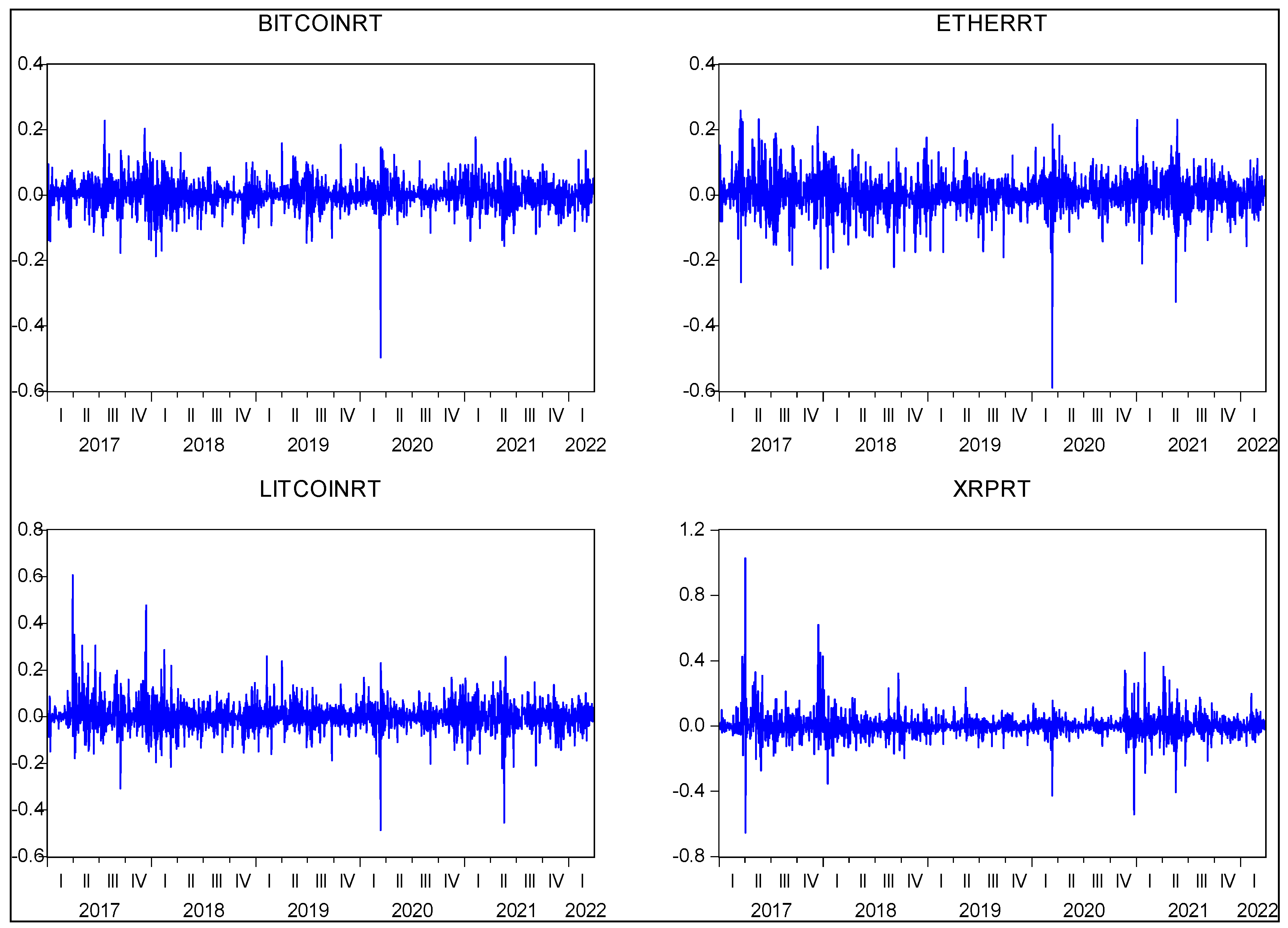
Figure 1. Daily Returns of Cryptocurrencies.
Jrfm 15 00513 g001
Figure 2. GARCH Values of Cryptocurrencies.
Jrfm 15 00513 g002
Figure 3. Dynamic Conditional Correlation.
Jrfm 15 00513 g003
Table 1. Market capitalization as on 30 June 2022.
CurrencyMarket Cap
BitcoinUSD 377.53B
EtherUSD 129.53B
LitecoinUSD 3.79B
XRPUSD 16.02B
Table 2. Descriptive Statistics of Cryptocurrencies.
BITCOINRTETHERRTLITECOINRTXRPRT
Mean0.20%0.32%0.18%0.26%
Median0.23%0.22%−0.03%0.00%
Minimum−0.4973−0.5896−0.4868−0.653
Maximum0.22760.25860.6071.028
Std.Dev.4%6%6%8%
Skewness−0.8444−0.60560.66001.8551
Kurtosis15.082711.987715.554332.6549
Observations1913191319131913
Jarque-Bera11,864.26555.7212,701.771,193.7
Probability0000
Table 3. Correlation Matrix of Cryptocurrencies Return.
BITCOINRTETHERRTLITECOINRTXRPRT
BITCOINRT1.0000
ETHERRT0.72101.0000
LITECOINRT0.68250.69311.0000
XRPRT0.46760.50830.52351.0000
Table 4. Holding Period Performance.
One-Year Return
BITCOINETHERLITECOINXRP
Mean175%595%1092%334%
Med61%65%24%22%
Max1832%14,171%44,380%6921%
Min−83%−92%−87%−93%
SD277%1733%4630%1075%
Three-Year Return
Mean78%86%36%31%
Med79%66%20%18%
Max149%267%280%178%
Min−0.12%−15.52%−56.74%−40.37%
SD34%74%67%45%
Five-Year Return
Mean94%133%96%63%
Med102%132%99%73%
Max121%239%171%108%
Min49%23%1%−1%
SD22%63%66%37%
Table 5. Unit root test.
BITCOINRTETHERRTLITECOINRTXRPRT
T Stat−47.051−46.831−46.98−30.04
Prob.0.00010.00010.00010.0001
Table 6. ARCH Effect.
BITCOINRTETHERRTLITECOINRTXRPRT
F-Stats9.797825.183636.7409133.5966
Prob.0.000.000.000.00
Table 7. Granger Causality among Cryptocurrencies.
Null Hypothesis:
Jrfm 15 00513 i001 Indicates Does Not Granger Cause
F-StatisticProb.Type of Causality
ETHERRT Jrfm 15 00513 i001 BITCOINRT8.53850.0002 *Unidirectional
BITCOINRT Jrfm 15 00513 i001 ETHERRT0.06230.9396No causality
LITECOINRT Jrfm 15 00513 i001 BITCOINRT1.06970.3433No causality
BITCOINRT Jrfm 15 00513 i001 LITECOINRT2.21980.1089No causality
XRPRT Jrfm 15 00513 i001 BITCOINRT4.66750.0095 *Unidirectional
BITCOINRT Jrfm 15 00513 i001 XRPRT0.65060.5218No causality
LITECOINRT Jrfm 15 00513 i001 ETHERRT0.23740.7887No causality
ETHERRT Jrfm 15 00513 i001 LITECOINRT0.93670.3921No causality
XRPRT Jrfm 15 00513 i001 ETHERRT2.94380.0429 **Unidirectional
ETHERRT Jrfm 15 00513 i001 XRPRT0.38210.6825No causality
XRPRT Jrfm 15 00513 i001 LITECOINRT0.58180.559No causality
LITECOINRT Jrfm 15 00513 i001 XRPRT1.15750.3145No causality
* Significance at 1% level; ** Significance at 5% level.
Table 8. ARIMA (1,1) Model.
BITCOIN RTETHER RTLITECOIN RTXRP RT
Coeff.Prob.Coeff.Prob.Coeff.Prob.Coeff.Prob.
c0.00150.10760.00240.04780.00120.36210.00200.2155
AR(1)−0.75080.0000−0.80530.0000−0.77990.0000−0.42350.1371
MA(1)0.71310.00000.76370.00000.74190.00000.36340.2148
Table 9. GARCH Model.
BITCOINRTETHERRTLITECOINRTXRPRT
Coeff.Prob.Coeff.Prob.Coeff.Prob.Coeff.Prob.
C0.00010.00100.00030.00100.00020.00100.00040.0010
ARCH ( α 1 )0.10080.00100.09270.00100.06730.00100.39230.0010
GARCH ( β 1 )0.83760.00100.79610.00100.87370.00100.63040.0010
Table 10. EGARCH Model.
BITCOINRTETHERRTLITECOINRTXRPRT
Coeff.Prob.Coeff.Prob.Coeff.Prob.Coeff.Prob.
α 0 −0.62230.001−0.53340.001−0.4380.001−0.76950.001
α 1 0.17010.0010.20750.0010.15570.0010.43780.001
λ−0.06490.001−0.02260.00310.02740.0010.06970.001
β0.92140.0010.93430.0010.94110.0010.91590.001
Table 11. GARCH-M Model.
BITCOINRTETHERRTLITECOINRTXRPRT
Coeff.Prob.Coeff.Prob.Coeff.Prob.Coeff.Prob.
Δ0.04130.73600.11860.31430.13630.33600.01820.7593
C0.00010.00100.00020.00100.00020.00100.00030.0010
A0.10090.00100.11280.00100.06780.00100.36260.0010
Β0.83730.00100.82230.00100.87250.00100.65380.0010
Table 12. Mean of DCC of Cryptocurrencies Return.
BITCOINRTETHERRTLITECOINRTXRPRT
BITCOINRT1.0000
ETHERRT0.72101.0000
LITECOINRT0.73790.74561.0000
XRPRT0.61430.68690.68181.0000
Table 13. DCC (1,1) Model.
Estimatet-ValuePr(>|t|)
All Currenciesα0.0337.8150.000
β0.963186.1980.000
Bitcoin–Etherα0.0582.3300.020
β0.93427.6970.000
Bitcoin–XRPα0.0373.3370.001
β0.95666.7370.000
Bitcoin–Litcoinα0.0483.6150.000
β0.94862.4680.000
Ether–Litcoinα0.0385.1630.000
β0.962128.7840.000
Ether–XRPα0.0342.8820.004
β0.96264.7870.000
Litcoin–XRPα0.0343.4210.001
β0.96586.3640.000
Publisher’s Note: MDPI stays neutral with regard to jurisdictional claims in published maps and institutional affiliations.