1. Introduction
Since the COVID-19 pandemic hit the world economy, many studies have revealed that energy-consumption patterns in various countries have been disrupted by the countermeasures, such as the lockdown, designed to prevent the spread of the coronavirus (
Bahmanyar et al. 2020;
Aruga et al. 2020;
D’Alessandro et al. 2021;
Rouleau and Gosselin 2021). In many countries that implemented lockdown measures, it is suggested that although domestic electricity demand increased when people spent more time in their homes, the overall electricity consumption decreased as business and physical activities shrank severely; the reduction in commercial and industrial demand was greater than the increase in the domestic demand (
Bahmanyar et al. 2020).
Studies examining the impact of the COVID-19 confinement measures implemented by governments on human mobility indicate that these measures significantly contributed to reducing human mobility (
Hadjidemetriou et al. 2020;
Santamaria et al. 2020). This reduction in human mobility related to COVID-19 is known to have decreased air pollution and levels of CO
2 emissions (
Orak and Ozdemir 2021;
Sifakis et al. 2021;
Aruga et al. 2021;
Archer et al. 2020) but few studies have investigated the context of how these changes in human mobility influenced energy demand. There are studies investigating the effects of COVID-19 on energy consumption (
Wang and Zhang 2021;
Carvalho et al. 2021;
Aruga et al. 2020), but these did not examine how changes in human mobility are related to energy consumption.
Aruga (
2021) examined the effect of the COVID-19 restrictions on fuel markets, such as gasoline and diesel, from the perspective of human mobility, but this study did not test the impact of these restrictions on electricity consumption. Furthermore, the study only tested the effects of the human-mobility index related to the transport sector, such as the changes in the numbers of visitors to transit stations and workplaces.
To fill this research gap, this paper aims to identify the difference in the effects of the types of human-mobility changes on electricity demand when the stay-at-home measures were implemented during the COVID-19 pandemic. To this end, this study investigates how the six human-mobility categories provided in the Google mobility data (
Google Inc. 2022) influenced the daily electricity demand during the pandemic. The six categories consist of percentage changes in the number of visits to retail and recreational sites, groceries and pharmacies, parks, transit stations, and workplaces, and the hours spent in residential areas compared to a baseline period (3rd January–6th February 2020) before the COVID-19 outbreak.
Up until the outbreak of COVID-19, no reliable data existed that captured changes in human mobility related to confinement measures to control human mobility. Thus, the mobility data during the COVID-19 pandemic offer a major opportunity to understand how restrictions on human mobility influence energy consumption. Since most countries still depend largely on fossil-fuel energy, improving energy efficiency by using less energy is an effective way to reduce greenhouse-gas emissions. Hence, this study provides important information to support the design of policies to enhance energy efficiency by controlling human mobility. The study also offers valuable information for policymakers seeking to reduce energy consumption by controlling human mobility by verifying the types of activities related to human mobility that increase energy consumption.
In the
Section 2, details of the data used in the study are explained. In the
Section 3, the empirical methods of the study are described. The
Section 4 discusses the results of the analyses conducted in the study, and the conclusion is drawn in the
Section 5.
2. Data
This study focuses on the case of Tokyo, Japan. Tokyo has the world’s busiest train station, Shinjuku (
Chowdhury and McFarlane 2022), ranked third in the world after London and New York in the Global Power City Index (GPCI) in 2021 (
Institute for Urban Strategies 2021), and is one of the cities with the greatest level of human mobility in the world. Thus, it is suitable for examining how the changes in human mobility related to the confinement measures during the COVID-19 pandemic affected energy consumption.
During 2020–2021, a state of emergency (SOE) was declared four times in Tokyo by the Tokyo Metropolitan Government. The length of each SOE period in Tokyo is presented in
Table 1. To avoid small sample sizes and, since the effect of the SOE measures, often lasted longer than the actual SOE period, the study included data for four weeks before and after the days when the SOE started and ended. When the third SOE ended, it continued through a measure called the ‘manen-boshi’ until 11 July 2021 (almost three weeks after the third SOE ended), a quasi-SOE measure that was not as severe as the SOE but did involve some restrictions during business hours for restaurants. It is probable that these quasi-SOE measures also influenced human mobility.
The confinement measures designed to cope with the spread of the coronavirus conducted under the SOE in Tokyo were similar to those in other countries. They included prohibiting large public events, limiting the business hours of shops, and requesting companies to enforce working from home; however, Tokyo was never subject to harsh lockdown regulations with severe penalties. The SOE measure was implemented when the number of daily COVID-19 cases increased.
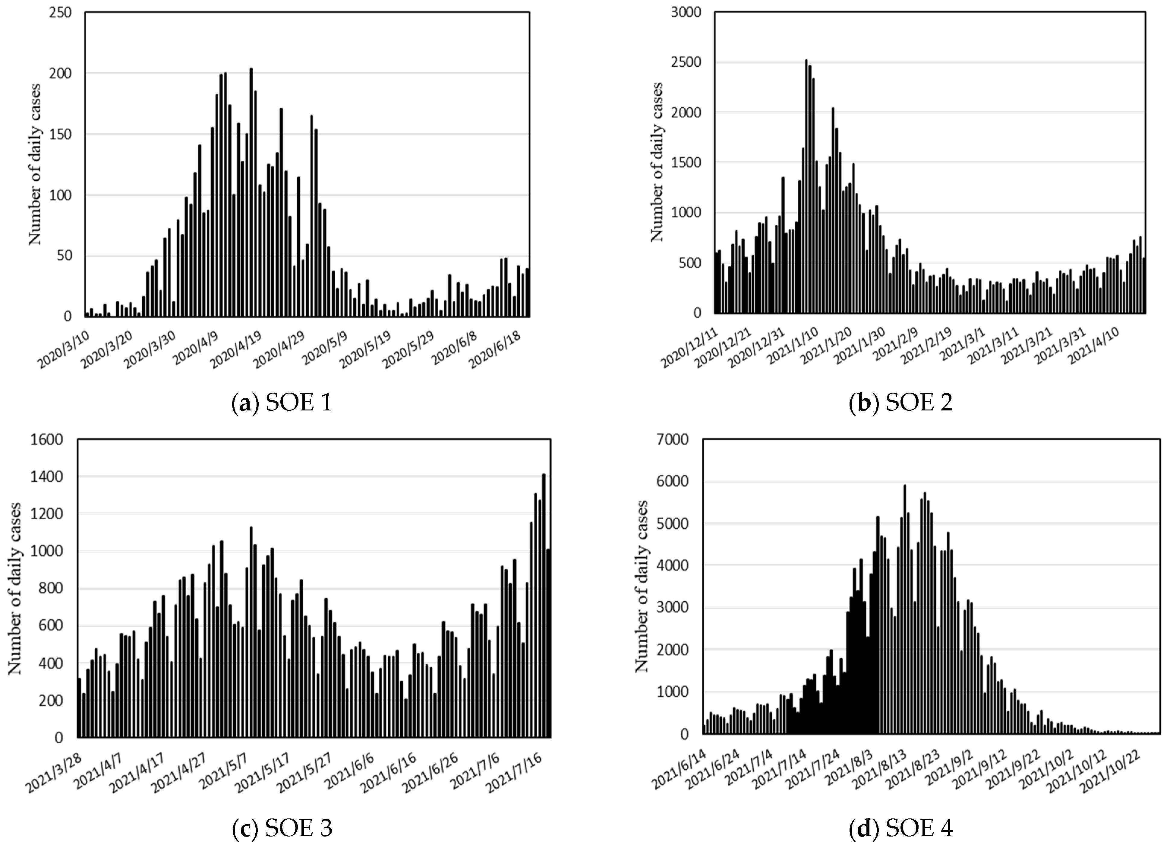
Figure 1 illustrates the changes in the number of daily COVID-19 cases during the four SOE periods. It is discernible from the figure that the number of COVID-19 cases declined for some time after the implementation of the SOE measures.
To capture the changes in human mobility during the SOE periods, six mobility indices were obtained from the Google mobility data (
Google Inc. 2022).
Table 2 describes the details of these mobility indices.
For the electricity-demand data, the average total daily electricity demand for the users of the Tokyo Electric Power Company (TEPCO) was used. The data were obtained from the homepage of
TEPCO (
2022). These demand data contained the total electricity demand covered by TEPCO, including both domestic and industrial energy demand. Since the original data were provided in hours, the hourly data were converted into total daily demand by summing the demand over 24 hours. The unit of the original electricity demand was provided in 10 megawatts (MW) and, for analysis purposes, the data were converted into gigawatts (GW).
Table 3 shows the summary statistics of the data used in the study. It is apparent from the table that the decline in human mobility was most evident in the first SOE period. The retail, transit, and work mobility indices had the lowest negative numbers, and the residential index had the highest percentage change, indicating that the effect of the SOE measure on reducing human mobility was most evident in the first SOE period.
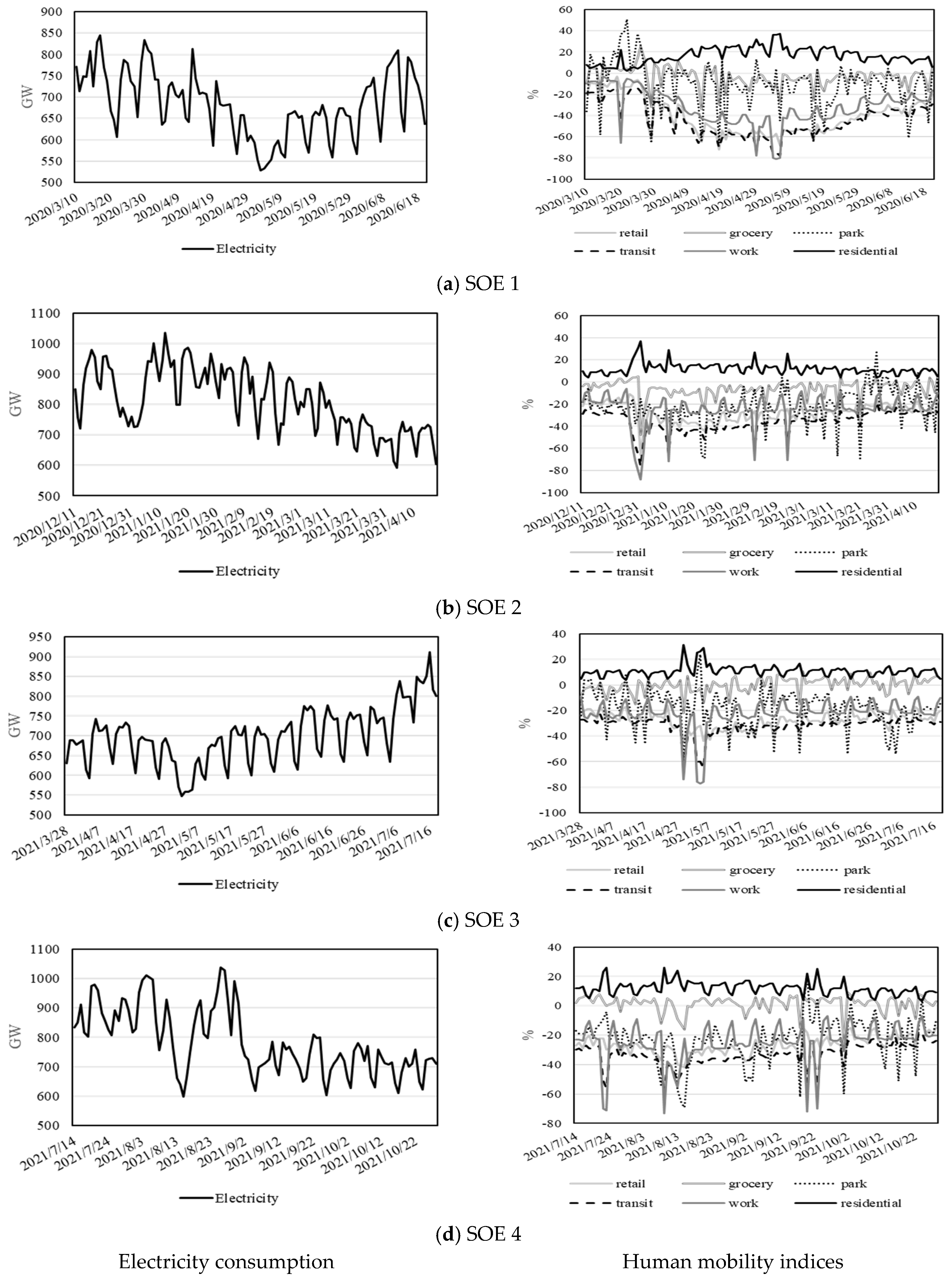
The difference in the data among different SOE periods is also presented in the plots of the electricity demand and human-mobility indices (
Figure 2). Here, it can be seen that the decline in the human-mobility indices was most apparent in the first SOE period. Furthermore, it is also discernible from the figure that in addition to the third SOE period, there were declining trends for electricity demand, which might have been related to the decrease in human mobility.
3. Methods
The study applied the following model for identifying the effects of changes in human mobility on electricity demand. The model is based on the model developed for analyzing the effects on CO
2 emissions (
Aruga et al. 2021):
where
electricity is the total daily electricity demand from the customers of TEPCO,
HM is one of the six human mobility indices,
before and
after are dummy variables containing days that are before and after the actual SOE periods, and
COVID is the daily cases of COVID-19 patients detected in Tokyo. The
before and
after dummies were included to consider the effects of days that were not within the actual SOE periods.
is the intercept,
through
are the coefficients of the independent variables, and
is the error term.
Since the sample size was relatively small in this study due to its focus on the state-of-emergency period, we used the autoregressive distributed lag (ARDL) model for the estimation. ARDL method is known for its strength in analyzing time-series data even when the sample size is small, and can prevent omission of variables and auto-correlation issues (
Pesaran et al. 2001). To capture the short- and long-term effects of the changes in human mobility on electricity demand, this study applied the following unrestricted-error-correction model:
where
p is the lag order for electricity demand and
q is that for the human-mobility indices. This equation was applied to the time-series data obtained for each four SOE periods (see
Table 1). The lag orders for the ARDL model are determined by the Akaike Information Criterion (AIC). Under the ARDL model, the bound test for cointegration was performed to determine the existence of a long-term relationship between the electricity demand and human-mobility indices.
The ARDL model requires the test variables to be integrated in order of zero or one (I(0) or I(1)). To confirm this before the ARDL model estimation, the study performed the Augmented Dickey–Fuller (ADF), Zivot–Andrews (ZA), and Kwiatkowski–Phillips–Schmidt–Shin (KPSS) stationarity tests. The ADF and KPSS tests were executed with both intercept and trend and the ZA test was conducted with a trend break.
To determine whether to apply the Newey–West heteroskedasticity and autocorrelation consistent (HAC) estimator (
Newey and West 1987), the study tested the existence of serial correlation and heteroskedasticity in the econometric models. For this purpose, the Breusch–Pagan–Godfrey (BPG) and Breusch–Godfrey (BG) tests were conducted. These tests were conducted using the model presented in Equation (2).
Table 4 summarizes these results for all SOE periods for each model. The results indicate that some models contained heteroskedasticity and autocorrelation; hence, to minimize these effects on the estimation, the study applied the HAC estimator. The stability of the ARDL model was also examined using the cumulative sum (CUSUM) and cumulative sum square (CUSUM square) tests. These test results suggested that most of our test models were within the 5% significance thresholds.
4. Results
To check whether the test variables were I(0) or I(1), the unit-root tests were conducted on all the variables for each SOE period. As shown in
Table 5, all the test variables were either I(0) or I(1), suggesting that the variables were suitable for applying the ARDL model.
To determine whether a long-term relationship was sustained between the electricity demand and six human-mobility indices during the four SEO periods, the ARDL bound test for cointegration was conducted.
Table 6 illustrates the results of this test. It is observable from the table that for all the models, the electricity demand and human-mobility indices had a cointegration relationship in all the SOE periods, suggesting the existence of a long-term relationship between these variables.
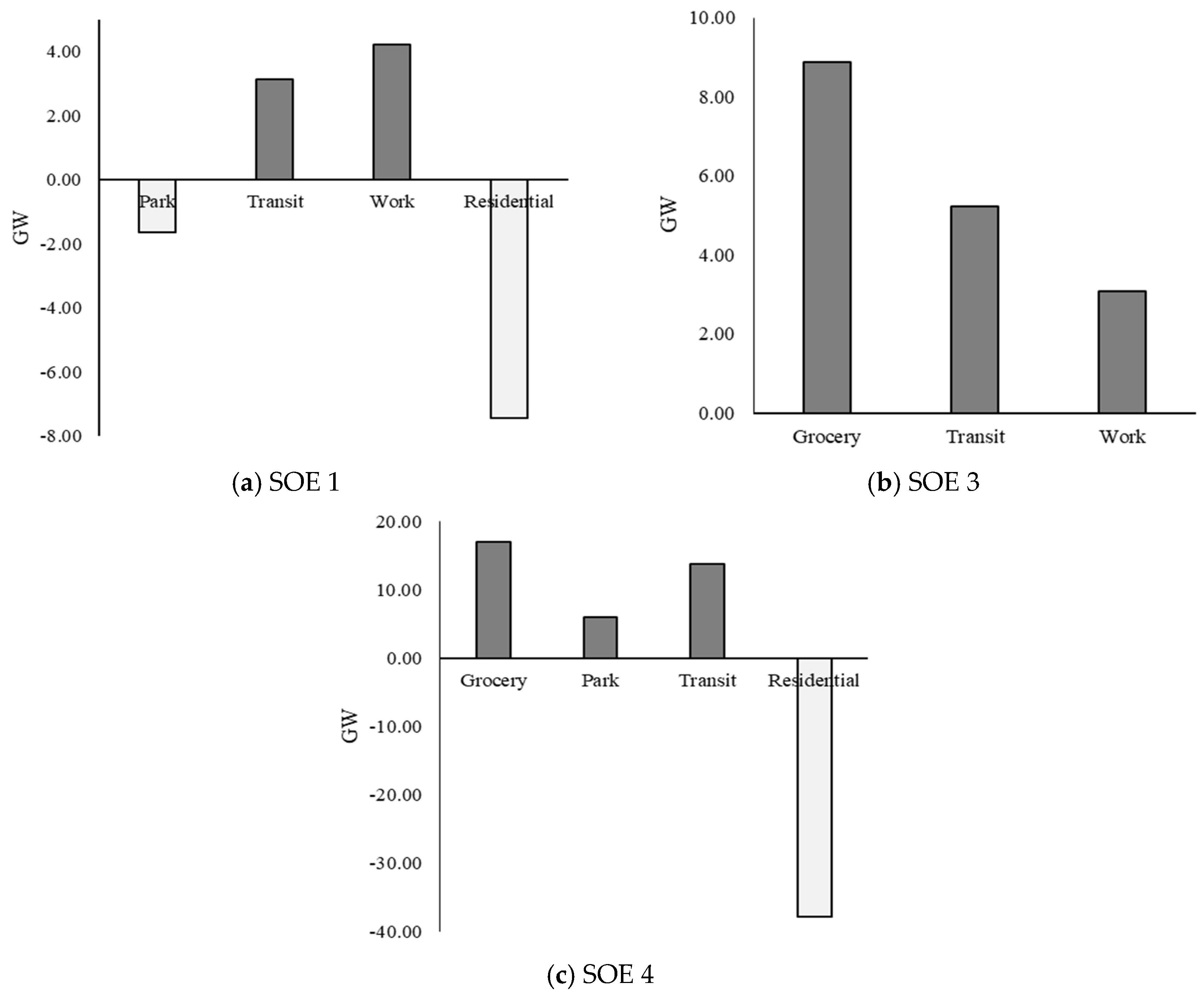
Table 7 shows the results of the ARDL long-term coefficient estimations. The table depicts whether the cointegration relationships were related to the effects of the six human-mobility indices. The results of the table imply that during the first SOE period, a percentage increase in the visits to park locations reduced the electricity demand by 1.64 GW, while an increase in the visits to transit stations and workplaces increased the electricity demand by 3.15 GW and 4.22 GW, respectively. It is also evident that a percentage increase in the hours spent in residential areas led to a 7.45-gigawatt decrease in electricity demand.
During the second SOE period, none of the human-mobility indices influenced the electricity demand, based on the 5% significance level. For the third SOE period, the human-mobility indices that became statistically significant all had a positive impact on the electricity demand. An increase in visits to groceries and pharmacies, transit stations, and workplaces all contributed to an increase in electricity demand. Finally, during the fourth SOE period, while groceries, parks, and transit stations had a positive impact on electricity demand, the hours spent at home had a negative impact on the demand. Intriguingly, while the park index had a negative impact during the first SOE, it became positive during the fourth SOE. This might have been related to the weakening of the effect of the SOE measure in the fourth SOE period. As shown in
Table 3, the average residential index was lower, and the retail, grocery, transit, and work indices were higher in the fourth SOE compared to the first SOE, indicating that the effect of the SOE on reducing human mobility was weaker in the fourth SOE period.
Figure 3 summarizes the long-term impact of the human-mobility indices on the electricity demand, whose coefficients were statistically significant at the 5% level, as shown in
Table 7. It is clear from the figure that changes in the hours spent in residential areas largely had an adverse effect on the electricity demand, while visits to transit stations had a positive impact on electricity demand in all three SOE periods. It is also evident from the results of the third and fourth SOE periods that the visits to grocery and pharmacy stores had the largest impact on boosting electricity demand among the six mobility indices.
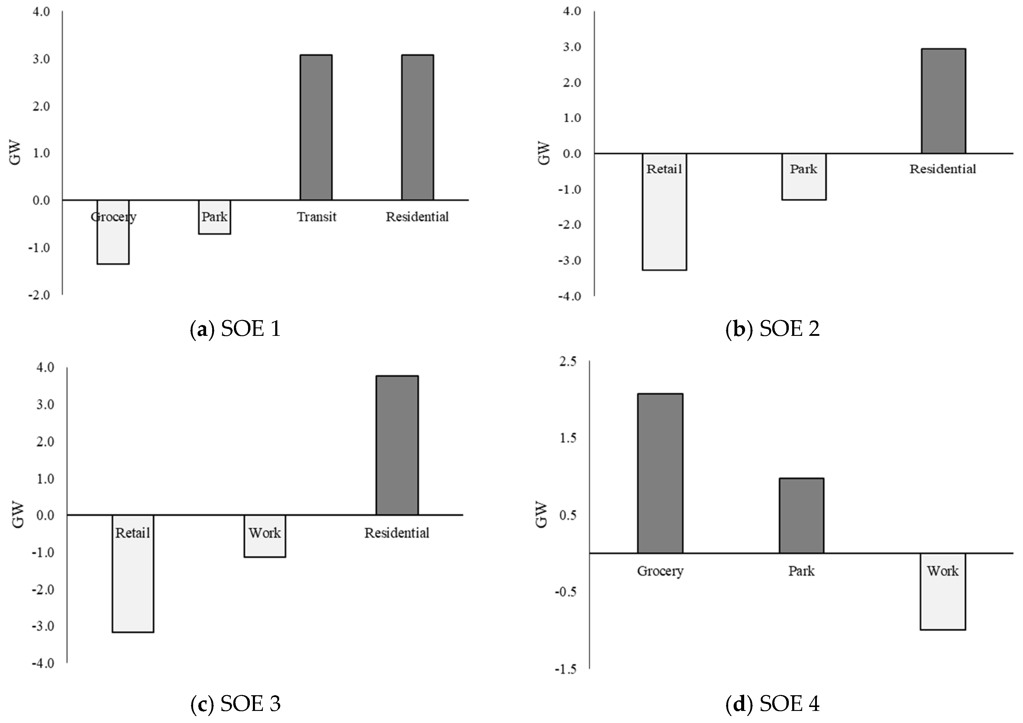
Finally,
Table 8 and
Figure 4 depict the results of the ARDL short-term coefficient estimations.
Figure 4 only presents the results when the coefficients for the human-mobility indices were statistically significant at the 5% level based on the results of
Table 8. The short-term coefficients denote the effect of the daily change in the human-mobility indices on the daily change in electricity demand. It is observable from the table and figure that the impact of the grocery and park indices on electricity demand had opposite signs between the first and fourth SOEs. Daily changes in visits to grocery and park areas had a negative impact on electricity demand in the first SOE period, but this effect became positive in the fourth SOE. As explained in the long-term results, the reason for this difference is likely to have been the weakening in the effect of the SOE on the reduction in human mobility in the fourth SOE.
It is also noticeable from the ARDL short-term coefficient estimations that daily changes in the residential index had a positive influence on the electricity demand. This result is consistent with the findings of
Bahmanyar et al. (
2020), according to which an increase in the number of hours spent at home contributes to an increase in the domestic energy demand. However, we should be aware that the long-term impact of the increase in the number of hours spent at home had an adverse impact on the electricity demand. This negative long-term impact is likely to have been related to a decrease in the energy demand in other areas than the residential district, such as office buildings, restaurants, and recreational locations, outweighing the increase in domestic demand as the length of time spent at home extended.
5. Conclusions
To identify how the changes in human mobility during the COVID-19 pandemic affected energy consumption, this study investigated the relationship between the changes in the number of people’s visits to various locations and electricity demand based on the case of Tokyo, Japan.
The study revealed that while an increase in the number of visits to groceries, pharmacies, and transit stations led to an increase in electricity demand, a rise in the hours people spent at home had a negative impact on electricity demand in the long run. Meanwhile, daily changes in the number of hours spent at home had a positive impact on daily changes in electricity demand, suggesting that there are times when domestic electricity demand contributed to increasing demand in the short run.
The study also demonstrated the differences in the effects of mobility changes on electricity demand among different SOE periods. While visits to park locations had a negative impact on electricity demand in both the long and short term during the first SOE period, they had a positive impact in the fourth SOE period. This result is likely to be related to the weakening in the effect of the SOE, since human mobility was higher, on average, in the fourth SOE period compared to the first SOE. This implies that when confinement measures become ineffective, electricity demand tends to increase along with human mobility.
Although further studies are required to identify the factors that lead to reductions in the electricity demand when hours spent at home increases during a SOE period, this study indicates that confining people to their homes for a certain period can contribute to reducing electricity demand. Thus, policies designed to shift people towards working from their homes when commuting to work is unnecessary might be an effective means through which to decrease energy consumption, and potentially, to help reduce greenhouse-gas emissions. Maintaining the energy balance between energy supply and demand is particularly important during crises and states of emergency, and this study provides useful information through which to understand how governmental regulation limiting human mobility can influence electricity demand. As the energy transition unfolds across the world, ensuring the optimization of integrated energy systems has never been more important; thus, the current study suggests that controlling human mobility could be one of the options through which policymakers could intervene in the energy-demand sector.


