Abstract
Cross-sectional data show Global North countries export higher quality products at a point in time. Product-level panel data can address if countries improve their export quality over time. The literature has addressed this practically relevant panel question only in small samples over the short term. We addressed it for a large sample, over the long run, focusing on the hitherto overlooked endogeneity between export quality and factor accumulation and the role of export composition. We utilized a two-tiered panel: the panel of countries and the panel of products each country trades. We found some evidence that middle-income countries often upgrade export quality within the same product, but that high- and low-income countries do this less often. Our results appear to support product cycle theory: some countries climb the value ladder, others are competed off from the ladder’s top, and new countries enter markets. Technology appears to be a potential basis for consolidating trade competitiveness over time, as skill accumulation becomes more widespread across countries and loses significance as an explanatory variable. Our results provide some explanation of why Global North countries might resist sharing technology. This research is timely with deadlocked multilateral trade negotiations and looming trade wars. It attempts to contribute to an evidence-based guide to trade policy.
Keywords:
export quality; factor accumulation; trade competition; economic development; technology competition JEL Classification:
F10; F14
1. Introduction
We intuitively expect the process of development to be reflected in the increasing sophistication of exports. Extant literature (e.g., Balassa 1979; Romalis 2004; Hallak 2006; Chor 2010; Hallak 2010; Costinot et al. 2011) has mostly utilized cross-sectional data to investigate this, thus shedding light only on what happens at a point in time. The only exception is a very brief panel section in Schott (2004). Also, studies of a single or a handful of countries over shorter periods exist in the literature (Schott 2002; Romalis 2004; Fabrizio et al. 2007; Verhoogen 2008; Khandelwal 2010).
Typically, we expect the increase in per capita income or rising capital and skill abundance, viz. the development process, to be reflected in the increasing sophistication of exports. This process may be driven by different factors depending on the level of an economy’s development. Rising income levels may create a demand for more sophisticated products, encouraging their production and sale domestically and abroad (Linder 1961). In addition, product cycle theory (Vernon 1966; Flam and Helpman 1987; Grossman and Helpman 1989; Grossman and Helpman 1991a) suggests that the process of increasing sophistication can arise from the transfer of technology into Global South countries. Transfer of technology leads to increasing competition among countries and further innovation. This implies rising sophistication of exports for all countries, no matter what their stage of development. Understanding the process could contribute to our understanding of how international competition among countries evolves at different stages of development.
In this paper, we add to the literature by asking a timely question of practical relevance. Specifically, with the availability of detailed product-level data (e.g., Feenstra et al. 2005), we can ask whether countries would improve their export quality over time as they develop and accumulate capital/skills/technology. Its timeliness arises from the current deadlock in negotiations of multilateral trade liberalization and the prospect of protracted trade wars (Regan and Barrett 2019; Baldwin 2016). The answers we seek will clarify how countries compete with each other over time as they develop. Greater clarity on this front will contribute to an evidence-based guide to trade policy, which is sorely needed in the current distrust of the multilateral system.
To study the long-term relationship between export quality and factor accumulation, we undertook a two-tiered analysis using a panel of countries first and then delved into the products that each country exports. We allowed the relationship to change with countries’ income and export composition because existing empirical results indicate that trade competitiveness depends on their position in the product value ladder and their income (Schott 2002; Khandelwal 2010). Moreover, the composition of exports changes countries’ trade competition strategies (Fabrizio et al. 2007). Trade competition strategy impacts the quality of exports that a country chooses to produce. Finally, we addressed the hitherto overlooked endogeneity between export quality and factor accumulation and proposed appropriate instruments.
Our findings indicated some interesting patterns. For example, middle-income countries most often upgrade export quality within the same product. In contrast, high-income countries do this less frequently, and low-income countries are the least likely to upgrade within the same product. Therefore, our results present evidence for product cycle theory. Middle-income production climbs up the product value ladder. High-income leaves as imitators compete them off the top of the value ladder, and low-income are new entrants into product markets.
Among our findings from the panel of countries is that factor accumulation’s role appears to change over time both in terms of significance and direction of influence. We find some evidence of the growing importance of technology as a means of successful participation in global markets, particularly in the manufacturing sector. We see that low-income countries often absorb technology from Global North countries (e.g., Barro and Lee 2001). Global North countries view this as a threat to their competitiveness (Alper et al. 2019; Jin and Takenaka 2019), leading to acrimonious trade relations: stalemates in multilateral negotiations (Payosova et al. 2018) and even trade wars. Our research provides an analysis of underlying trends that might provide a basis for understanding practical issues in international trade today. Our findings attempt to offer a nuanced guide to competitiveness considerations based on a country’s factor accumulation level. Thus we attempt to provide an alternative to trade policy based on politics (Mason 2019) by informing trade policy with economic fundamentals-based research.
2. Literature Review
Previous work has investigated the association of export quality and economic development at a point in time in a cross-sectional sample of countries (e.g., Schott 2004; Romalis 2004; Aiginger 1998) or they have pooled data across countries to find the average association of unit values of exports and measures of development over time (e.g., Schott 2004). The contribution of this paper is to investigate this question at the level of each country over time. Our approach thus allows us to make distinctions among countries based on their level of development.
Balassa (1979) estimated that the relative export performance of countries within individual product categories was significantly determined by the countries’ physical and human capital endowments. He contends that if these results are used to predict the future export structure given projected future values of countries’ physical and human capital, then as physical and human capital grow, Global South countries’ exports could supplant the exports of countries that graduated to a higher level. Relative export performance in Balassa (1979) is based on a measure of market share in a product as a ratio of average market share in other products involving the total exports of a country in each four-digit SIC category of manufactured products (resulting in 184 product categories) in the year 1972.
Romalis (2004) found similar results using 1998 data on U.S. imports categorized into four-digit SIC product categories. Specifically, he found that the market share of the rich trade partners of the U.S. rises within each product category with increasing factor intensity of capital and skilled labor.
The two above studies thus provide indirect evidence of a potentially changing pattern of cross-country participation in trade as countries grow and graduate to higher skill and capital endowments. There is some evidence of this in studies such as Khandelwal (2010), which found that the U.S. can continue to compete in products with low-wage countries where there is a scope for upgrading into more sophisticated versions, i.e., products with longer quality ladders. In products with shorter ladders, the U.S. industry is hurt by import penetration. Schott (2002) found more direct evidence of the process of countries graduating to higher levels of quality within a product using U.S. export and import data at the product level. He found that, during the 1990s, U.S. exports declined in product categories with the rise of competition from low-wage countries. He also found that U.S. intra-product trade with low-wage countries typically involves the U.S. selling a significantly higher unit value of the same product than it buys from low-wage countries. Schott (2002) contends that taken together, this provides evidence of a product cycle theory process where Global North countries invent and Global South countries copy (real world examples are in Radjou et al. 2012). This forces Global North countries to either innovate further through vertical differentiation in the same product or exit the market. Firm-level data confirm this sort of adjustment in U.S. manufacturing from 1977 to 1997 (Bernard et al. 2006).
Schott (2004) contends that countries predominantly specialize within products (defined as H.S. 10-digit classification) with a positive relationship between the product’s unit value and relative factor endowments of the exporting country. Taking this train of reasoning forward, in Balassa’s (1979) fashion, this would imply that over time as countries graduate to higher levels of skill and capital endowment, we could expect to see corresponding graduation to higher unit value levels.
This paper investigates the relationship between the unit value of exports of countries and their changing skill and capital endowments over time. It would be interesting to see if the type of vertical differentiation that the U.S. is found to practice in the face of low-wage foreign competition (e.g., Bernard et al. 2006; Khandelwal 2010; Schott 2002) is also practiced by countries in the process of their development. Vertical differentiation could be the result of competition from still lower-wage producers, as implied by, e.g., Bernard et al. (2006), Khandelwal (2010), and Schott (2002), and the natural evolution of production processes shaped by changing endowments, as implied by, e.g., Romalis (2004) and Balassa (1979).
The predictions of the Heckscher–Ohlin model indicate that the product using the abundant factor in a given country will be exported. As countries develop, human and physical capital increases (Barro 1991; Mukerji and Struthers 2021), implying that the relatively abundant factors will produce more technologically sophisticated output. With this change, we expect countries that develop to capture a greater share of the world markets in products that reflect their changing factor abundance at home (Romalis 2004).
Romalis (2004) deals with the quasi-Heckscher–Ohlin effect: countries will capture a larger share of production and trade in products that use their abundant factor more intensively. The quasi-Heckscher–Ohlin effect thus relates to our aim of testing whether changing factor abundance over time leads to changes in trade composition. This paper looks for evidence to corroborate this shift of factor abundance to a change in export unit values within products.
With changing factor abundance, we may expect many related changes. For instance, countries could climb up the value ladder in products they already export, thus utilizing their growing endowments of skill and capital. Alternatively, countries could migrate to the production of new products that are more skill- and capital-intense in production (e.g., Romalis 2004; Balassa 1979). Thus, while there are many issues involved in changing factor abundance and its impact on trade, this paper focuses only on whether changing factor abundance is associated with changes in unit values exported within product categories.
In addition to the above evidence, empirical analyses of changing technology sophistication of exports based on Global South country case studies have corroborated the link between economic development and growing export sophistication. For example, Verhoogen (2008) found that exporting firms in Mexico pay their workers higher wages, and takes that as indirect proof that exporters are upgrading the quality of their output. Fabrizio et al. (2007) studied eight central and east European countries (CEE-8) between 1994 to 2004, as they transitioned from centrally planned economies through privatization and restructuring. They found that exports increased in products where these countries increased quality of output. They also found that the composition of the export basket changed in favor of more technology-intensive products. For seven countries that rapidly grew from 1960 to 1998, Romalis (2004) calculated a shifting pattern of market share, with these countries’ market shares exhibiting the positive correlation with capital and skill intensity after they had grown and graduated to the club of the “North” countries.
We found that less than a third of countries made the transition up the unit value ladder in their exports during the sample period (1972–2001), while the proportion is somewhat larger in the later years of the sample. The lowest proportion of products exported by low-income countries made this transition compared to those in the high- or middle-income categories.
For low-income countries, the increasing sophistication of exports might show up in the export of new goods instead of a rising price of existing imports. This paper focuses on within-product changes of real unit value experienced by a given country. While the increase in the real unit value of a product exported by a country could signify an increase in its export sophistication, it need not be the only avenue through which improved production capability manifests itself. The export of entirely new products is, in fact, another common manifestation of rising sophistication. New products trade is called the extensive margin of trade and is consistent with product cycle theory. For instance, low-income countries might start exporting new goods based on technology transfer from abroad. Mukerji (2013) found evidence of the greater importance of the extensive margin in trade growth among low-income countries related to technology transfer. In addition, competition, resulting innovation, and technology-driven cost saving might all drive down the price of existing exports (Helpman and Krugman 1985). Lower export prices would result in observed negative relationships over time.
One potential implication of the literature outlined above is that countries’ exports will change with growing capital/skill/technology abundance, i.e., the factor accumulation that accompanies economic development. Our paper aims to provide a direct test of this implication in a large sample of countries between 1972–2001.
We have chosen our period of analysis to capture the steepest acceleration in world trade as a percentage of world GDP since the Second World War (Fouquin and Hugot 2016). A mix of repeated rounds of multilateral trade liberalization through the General Agreement on Tarriffs and Trade (GATT) and the expansion of participation by countries at all levels of income led to the acceleration gathering steam in this period. Therefore, the sample starts in the early 1970s. The end time of 2001 is specifically chosen to restrict the sample to the period before China entered the WTO. We hope by doing so to capture the trade competition, especially among Global South countries, before this significant change. This paper aims to capture the impact of changing fundamentals of a country, represented by factor accumulation, on its trade. However, China’s entry had a considerable impact on trade in Global South countries which was not directly related to the fundamentals of these economies. For example, Brambilla et al. (2010) illustrate China’s outsize impact in competition faced by Global South countries.
3. Trends in Product-Level Export Unit Values
To estimate the relationship between exporting countries’ quality of exports and their factor accumulation over time, we used the unit values of product exports from the rest of the world to the U.S. to measure product quality; and capital per worker, education, and technology to measure factor accumulation. Table 1 details the definitions and sources of the data.

Table 1.
Data definitions and sources.
Using exports to the U.S. has the advantage of being available in product-level detail for a long time and spanning a vast majority of countries globally, thus allowing the study of export unit values at a practically helpful level of disaggregation. Moreover, since the U.S. accounts for a substantial share of world commerce, we can be confident in capturing a reasonable representation of each country’s exports. Trade with the U.S. is assumed to be fairly representative of trade for a given country because the U.S. figures among the top ten trading partners for close to 80% of all countries listed in the WITS trade database of the World Bank. Appendix C presents top ten trade partners of all countries in the World Bank database in along with an analysis of the role of the U.S. It is therefore not surprising that there are several prominent precedents in the literature of using trade with the U.S. as representative of a country’s overall trade, due to its high quality and detailed nature. See, for example, Schott (2004).
Table 2 presents the average percentage of products that have increased in real unit value (unit value deflated by the consumer price index) over the sample period. We categorized our findings based on income levels. For example, during 1972–1988, 29% of products that a high-income country exported in 1972 exhibited rising real unit values. As discussed in the introduction to this paper, changes in factor accumulation might improve the output quality and move production towards more capital/skill/technology-intensive products. Thus, Table 2 captures improvements in the quality of both existing and new exports.
Table 2.
Change in real unit values by country categories.
Table 3 presents the trends in real unit values by SITC classification. During 1972–1988, among manufacturing products (SITC 5 through 8), which most closely reflect exporter capital, skill, and technology abundance (Schott 2004), the trend of rising real unit values is present, on average, among 25% of products. It is 31% among the rest of the products. During 1989–2001, they rise in 32% and 26% of the cases, respectively. Given differences across SITC products, we realize that the composition of exports will play a role in the relationship between factor accumulation and export quality as measured by its unit value. We incorporate this finding in our analysis in the next section by controlling for differences in export composition.
Table 3.
Change in real unit values by SITC categories.
Both Table 2 and Table 3 illustrate that unit values are not increasing for all products as one might expect. The extant literature provides some basis for why this might be the case: price competition might be eroding the gains from quality improvement in the unit value of exports. For example, in calculating pure price indices that abstract from the changing quality over time, Hallak and Schott (2011) found that a flat unit value might hide a rising quality and falling prices, e.g., in the case of south-east Asian economies in the early 2000s.
This raises the broader question of the difficulty of capturing changes in export quality over time when economic forces manifest themselves in changes in competition, cost of production, inflation, exchange rate fluctuations, etc. This paper attempts to control for these economic forces through our data and estimation strategies. For example, we use appropriate controls in the regressions, we deflate export prices, we conduct robustness checks that account for changing composition of trade, and changing values of the home currency. All this ensures that our results are reasonably robust to these factors.
4. Empirical Analysis
In this Section 4.1 presents the data, the variables used in the regression, and the estimation strategy. Section 4.2 and Section 4.3 lay out the formal regression equations that were estimated.
4.1. Estimation
The data-set we used was a panel of countries over the time period 1972 to 2001. In turn, each country’s data contained a panel of products exported to the U.S. We utilized the two-tiered structure of our panel data by analyzing the panel of countries and a separate analysis for each country with the panel of products it exports. The regression equations used in these two analyses are presented in Section 4.2 and Section 4.3 below, specifically in Equations (4) and (5), respectively. In both analyses, we used a first differenced instrumental variables regression to study the relationship between factor accumulation and export quality.
We used the real unit value of exports as a measure of export quality and included interactions between product-SITC and year dummy variables to control market-specific trends. Hummels and Klenow (2005) contend that export unit value differences predominantly embody quality differences. Indeed, using unit values to measure export quality has considerable precedence (e.g., Aiginger 1998; Hallak 2006; Schott 2004). However, Hallak and Schott (2011) have pointed out potential problems with this approach due to differences in production cost and possible currency valuation problems. We address these issues with an additional estimation using the exporting country’s domestic currency as units instead of the U.S. dollar. The unit values are deflated by the exporter country’s wholesale price index1 in this case.
The explanatory variables are exporter characteristics that capture factor accumulation: real capital per worker, education level of labor (to measure skill), and real per capita gross domestic product (to measure technology). We included interaction terms between factor accumulation and composition of exports to allow factor accumulation’s relation to export quality to change based on the composition of exports. For example, Schott (2002, 2004) and Khandelwal (2010) show countries compete in export markets by upgrading export quality. Fabrizio et al. (2007) investigated changing export composition among eight central and eastern European countries in the decade leading up to their entry into the E.U. in 2004.
A discussion of causality is relevant for our regressions because extant literature (e.g., Verhoogen 2008; Baldwin and Gu 2003) provides a theoretical and empirical basis for the potential of upgrades in export quality (which is our dependent variable) leading to future spillovers to the rest of the economy. Therefore, factor accumulation, which is our independent variable, may be correlated with past export quality. For example, other sectors learn from exporters, leading to technology upgrades to the rest of the economy in the future. Here, we have a potential for reverse causality from our dependent variable to future values of our independent variables. At the same time, the current factor accumulation determines the current period’s export quality. Our data could thus be reasonably assumed to be sequentially exogenous (Wooldridge 2010). It is useful to illustrate our assumption of sequential exogeneity in a simple panel data setting, where are the independent variables, is the dependent variable, is the error term, and is the unobserved panel effect (in our case, the country effect and product effect for the panel of countries and the product effect for the panel of products):
where and
When (2) holds, we say, are sequentially exogenous conditional on the unobserved effect . Given the model in (1), we write assumption (2) as:
From (3) we see that sequential exogeneity implies that after we control for and , no past values of affect the expected value of . This assumption allows for the practical possibility that future values of (factor accumulation variables) are correlated with the current (export quality) due to spillover from upgrades from the export sector to the rest of the economy. Sequential exogeneity leads to inconsistent estimation of (1), thus we used differencing combined with an instrumental variable approach for consistent estimation (Wooldridge 2010). Equation (2) implies that lagged values of the independent variables are valid instruments for contemporaneous independent variables. We used two lags of independent variables as instruments.
4.2. Data
Export data are taken from the Bureau of Census of the U.S. and are compiled by Feenstra et al. (1997) and updated in Feenstra et al. (2005). The data cover the period 1972–2001. In 1972–1988, U.S. imports are measured according to the Tariff Schedule of the United States Annotated (TSUSA) classification. Between 1989 and 2001, imports are measured by the Harmonized System of Commodity Classification (HTS 10-digit product data). Thus our analysis is separate for the two subsample periods: 1972–1988 and 1989–2001.
The data provide the quantity (for example, meters of cloth, tons of steel, or the number of shirts) and the dollar value of the United States trade with partner countries for each of the thousands of TSUSA and HTS classified products. Using the quantity and value associated with a product’s trade, we calculated each product’s unit value and used it to measure quality.
We used three measures for a country’s factor accumulation (similar to extant literature, e.g., Balassa 1979; Romalis 2004; Schott 2004). Capital abundance was measured by real capital per worker taken from the Penn World Tables (Mark 5.6), compiled by Summers (1995). Skill was measured as the population share attaining secondary or higher education, and the level of technology was measured using real per capita gross domestic product. Both the skill and technology measures were from the World Development Indicators of the World Bank. Table 1 details the definitions and sources of the data.
4.3. Panel of Countries: Empirical Analysis and Data
We estimated the relationship between factor accumulation and export quality using the panel of countries. One of the benefits of this estimation is that we can control for unobserved factors that vary over time across product markets, for example, trends in consumption that might make the demand for a product change. The sample comprised a maximum of 122 and 152 trading partners of the U.S., respectively, during 1972–1988 and 1989–2001. The data were annual, and we estimated separately for the two time periods since the product classifications are TSUSA in 1972–1988 and H.S. 10 in 1989–2001. The countries included in the regression depended upon data availability of factor accumulations, and we list them in Appendix A.
We estimated the following first differenced regression, using pooled two-stage least squares and two lags of factor accumulation as instruments. The estimated equation is:
where is the first difference, is the natural log following the literature (e.g., Balassa 1979; Schott 2004; the coefficients thus are interpreted as elasticities), is the real unit value of export of product m, for country c, in year t, stands for the particular measure of country c’s factor accumulation in period t for which we use the following, one at a time to avoid multicollinearity issues: real capital per worker, education level of labor (to measure skill), and real per capita gross domestic product (to measure technology), Low inc stands for low income, and is the corresponding error term. is interacted with dummies for low- and high-income countries (Low inc and High inc, respectively) and predominant exporters of manufacturing, services, or fuel (Manf. exp, Serv exp and Fuel exp, respectively). These interactions formally test the hypothesis we presented in Section 4.1, namely, that the impact of changing factor accumulation might be differentiated by export composition. In estimating Equation (4), we included time and product category (SITC) dummies. Finally, to control for unobserved factors that vary over time across product markets, we included interactions of time and product-SITC dummies. is sequentially exogenous, leading to inconsistent estimates, so we use and as instruments to ensure consistency.
The panel estimation yields two vectors of coefficients—one each for 1972–1988 and 1989–2001, respectively. We discuss the results in Section 5. Standard errors are adjusted for serial correlations and heteroscedasticity. Following each panel estimation, the test of overidentifying restrictions was used to test the validity of our assumption of sequential exogeneity. Sequential exogeneity is supported, as we fail to reject the null that the errors are uncorrelated with our instruments.
Measurement error problems might arise in the form of errors in measuring the unit values of U.S. imports (dependent variable) and errors in measurement of country characteristics (independent variables). We considered measurement error in the dependent variable first. Since U.S. authorities collect data on U.S. imports, we can reasonably assume that our dependent variable’s measurement error is independent of the country that exports the product to the U.S. Therefore, the estimation is consistent even if such measurement error was present. Measurement error in the independent variables implies that country characteristics are measured with an error. It is likely that country characteristics were measured with greater accuracy in richer, more developed countries. Thus the measurement error is correlated with the true independent variables; the more advanced the country, the lower the measurement error, and uncorrelated with the observed independent variable. Accordingly, the classical-errors-in-variables model does not apply to our estimation, and therefore our estimation will produce consistent results (Wooldridge 2010).
4.4. Panel of Products: Empirical Analysis and Data
The sample comprised 122 and 152 exporting countries in 1972–1988 and 1989–2001, respectively. The estimation was then undertaken for each country separately, utilizing the panel of products over time that each country exports to the U.S.
The estimated equation for each country c is:
where stands for taking the first difference, is the natural log, is the real unit value of export of product m, for country c, in year t, stands for measures of country c’s factor accumulation in period t for which we use: real capital per worker, education level of labor (to measure skill), and real per capita gross domestic product (to measure technology), and is the corresponding error term. In estimating Equation (5), we included product category (SITC) dummies. Additionally, to control for unobserved factors that vary over time across product markets, we included interactions of time and product-SITC dummies. Similar to our previous estimation strategy, the regression in (5) was estimated for a given country’s panel of products by pooled two-stage least squares using two lags of the independent variables as instruments. Specifically, is sequentially exogenous, leading to inconsistent estimates, so we use and as instruments to ensure consistency. This estimation yielded 122 and 152 coefficients for 1972–1988 and 1989–2001, respectively. Standard errors were adjusted for serial correlation and heteroskedasticity.
We presented our data and estimation strategy in this section. We will interpret our results in the next section.
5. Results
5.1. Panel of Countries
The results of estimating the regression in Equation (4) are in Table 4, Table 5, Table 6, Table 7 and Table 8. Table 4, Table 5 and Table 6 present the results for 1972–1988, and Table 7 and Table 8 present the results for 1989–2001. Table 4 presents the results of 1972–1988 of the panel of countries when skill and its interaction with country income and export composition are the independent variables. Rising skill level is associated negatively with real export unit value growth; the elasticity is −0.51. Thus a two standard deviations increase in skill level is associated with a 32% decrease in unit values. This is fairly significant from a practical standpoint. However, there are two exceptions—low-income countries with an elasticity of 0.23, and service exporting countries with elasticity 0.58—where improvement in skill has a positive impact. Simply being a high-income country positively impacts, while at the average level of skill accumulation, being a service exporter has a negative effect, albeit these are not economically significant at elasticities of 0.02 and −0.01, respectively.
Table 4.
Panel regression of countries, estimating Equation (4). Dependent variable: first difference of log real unit value of exports. Measure of factor accumulation: skill (log population share attaining secondary or higher education). Years: 1972–1988.
Table 5.
Panel regression of countries, estimating Equation (4). Dependent variable: first difference of log real unit value of exports. Measure of factor accumulation: capital (log capital per worker). Years: 1972–1988.
Table 6.
Panel regression of countries, estimating Equation (4). Dependent variable: first difference of log real unit value of exports. Measure of factor accumulation: technology (log per capita gross domestic product (PCGDP)). Years: 1972–1988.
Table 7.
Panel regression of countries, estimating Equation (4). Dependent variable: first difference of log real unit value of exports. Measure of factor accumulation: skill (log population share attaining secondary or higher education). Years: 1989–2001.
Table 8.
Panel regression of countries, estimating Equation (4). Dependent variable: first difference of log real unit value of exports. Measure of factor accumulation: technology (log per capita gross domestic product (PCGDP)). Years: 1989–2001.
Table 5 presents the results of 1972–1988 of the panel of countries when the independent variable is capital and its interaction with income and export composition. Overall capital growth was positively correlated with growth in real export unit values with an elasticity of 0.42, which translates to an approximately 50% rise in unit values with a two standard deviation change in capital stock per worker from its mean. However, rising capital was associated negatively with real unit value growth for low-income countries with an elasticity of −0.11. At the average capital accumulation, being a low- or high-income country adds positively to the growth of unit values. Here, too, the elasticities were too small in magnitude to be of practical significance at 0.01 and 0.03, respectively.
Table 6 presents the results of 1972–1988 when the independent variable is technology, and its interaction with income level and export composition. Technology improvement was positively correlated with real unit value with an elasticity of 0.9, which implies a rise in unit values of 120% with a two standard deviation change in technological improvement from its mean. Interestingly, this relationship was even stronger in high-income countries where the elasticity was 1.6, while it is smaller in magnitude in low-income countries where the elasticity was 0.07. In contrast, service exporter countries saw a negative correlation with technological improvement where the elasticity was −0.32. Being a low-income country or a service exporter adds positively to the growth of unit values. However, the elasticity was not economically significant at only 0.01 for both.
Table 7 and Table 8 present the results for 1989–2001. Table 7 shows results of 1989–2001 when the independent variable is skill, and its interaction with income and export composition of countries. None of the variables had any significant impact here. Table 8 presents the results of 1989–2001 when the independent variables are technology, and its interactions with countries’ income and export composition. Technology seemed to have a negative relation with the growth of unit value as the elasticity was −0.25, which represents a fall in unit value of 37% for a change in technology of two standard deviations from its mean. For manufacturing exporters, improving technology was associated with a smaller negative impact with an elasticity of −0.14. The impact for fuel exporters was the largest in magnitude and positive with an elasticity of 0.29. Being a high- or low-income country has a slight negative impact on real unit value growth.
In summary, in the sample period 1972–1988: skill growth decelerated growth of real export unit values. Low income and service exporters were exceptions here, as skill growth led to accelerated growth of unit values in such countries. Capital growth accelerated growth of real export unit values except in low-income countries where it was associated with deceleration. Technology growth accelerated the growth of real export unit values, most especially in high-income countries. There was much less acceleration in low-income countries, while there was a deceleration in service exporters.
In summary, in the sample period 1989–2001: technology growth was associated negatively with unit value deceleration, although much less so in manufacturing exporters, and accelerated it in fuel exporters. Skill no longer had any significant impact.
Over time it appears that skill accumulation has receded in importance as a significant differentiator. While in the earlier time period, at least low income countries saw gains in unit value from skill improvement. This is no longer significant in the latter time period. One reason could be the spread of education across all countries. For example, Global South countries in general and particularly countries in Sub-Saharan Africa and the Middle East/North Africa have shown robust progress in education skills in the latter time period (Barro and Lee 2001). Higher education levels the playing field and reduces the differences based on skill although it can have profound effects on competition based on technology (Grossman and Helpman 1991b), which we discuss next.
We saw that technological improvement was associated with growing real export unit values in the earlier period while this trend was reversed in the later period. Our results also indicate that manufacturing exporters’ real unit values decelerated much less. It appears that being a manufacturing exporter leads to benefits from technological advancement. One explanation could be that manufacturing has shifted from the high income countries, and middle- and low-income countries are benefitting from the transfer of technology in manufacturing. This supplanting of lower income countries in areas of higher income production was predicted by Balassa (1979). It is also supported by the findings of Khandelwal (2010) that higher income countries are competed off the value ladders in products where these ladders might be short. Finally, it is in line with evidence of innovations being copied across borders in Schott (2002). Certainly the skill gains from education could have helped in this technology transfer, as highlighted in Barro and Lee (2001).
Thus, our findings provide potential support for the product cycle theory where lower income countries catch up with higher income countries through technology transfer. This catch-up can be alarming as it cascades into large leap-frogging by lower income countries. Interestingly, much of the discord in international relations comes from Global North countries resisting sharing their technology. Our results provide some clues to the underlying mechanism for this emerging discord.
5.2. Panel of Products
The results of estimating Equation (5) are in Table 9, Table 10, Table 11 and Table 12. Each table’s cell gives the proportion of countries with a significant regression coefficient on the factor accumulation variable. For example, in the first cell, six out of 23—approximately 25%—of high-income countries, in 1989–2001, have a significant positive coefficient on skill-accumulation. In this case, our measure of export quality is the dollar unit value deflated by the United States consumer price index in Table 9. The rest of the table covers the entire range of income levels, factor accumulation measures, time periods.
Table 9.
Results summary *—panel regression of products, estimating Equation (5) with an unrestricted sample of products.3
Table 10.
Results summary—panel regression of products, estimating Equation (5) with an unrestricted sample of products.
Table 11.
Results summary—panel regression of products, estimating Equation (5) with sample restricted to products that were traded in the first year of the sample.
Table 12.
Results summary—panel regression of products, estimating Equation (5) with products restricted to those that belong to SITC 5–8 only.
Table 10 presents the regression results when the home currencies value exports. Table 11 and Table 12 present two robustness checks of the estimation of Equation (5). Table 11 estimates Equation (5) while restricting the products for each year to only those exported by the country in the first year of the sample. We aimed to abstract from the changing composition of trade due to entry into new markets or the invention of new products, and focused exclusively on the evolution of export quality within each existing product market. Table 12 contains the results of estimating Equation (5) while we restrict the exported product sample to SITC categories 5–8 only. These products are manufacturing exports, and hence they are most likely to be influenced by capital, skill, and technology accumulation of the exporter country (Schott 2004).
That unit values did not necessarily rise with improving factor abundance might be explained by innovation, falling prices, and technology-driven cost saving. We would see less positive relationships as unit values would not necessarily keep pace with factor accumulation. Hallak and Schott (2011) found that a flat or declining unit value might hide rising quality and falling prices, thus appearing to show that price competition might be eroding the gains from quality improvement in the unit value of exports. Therefore, we focused on the positive coefficients as a more precise measure of quality improvements over time.
We used graphs 1 through 5 to bring out the variations in results based on the different income levels. The statistical significance4 of the difference is below each chart. Figure 1 and Figure 2 show the percentage of countries with a positive significant coefficient on skill accumulation. Similarly, Figure 3 and Figure 4 plot the share of countries with a positive significant coefficient on technology accumulation. Figure 5 presents the capital accumulation results. The results are grouped based on the sample of products: all, manufacturing only, or those exported in the first year.
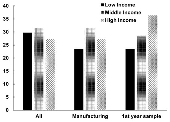
Figure 1.
Panel regression of products, estimating Equation (5). Percentage of countries with positive significant coefficient on skill-level: 1972–1988. The difference between income levels’ results, are statistically significant in all three categories of All, Manufacturing, and 1st year sample.
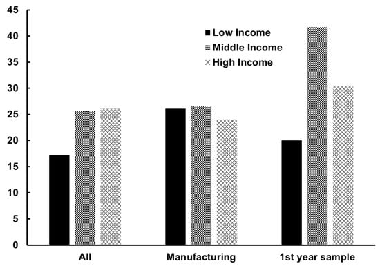
Figure 2.
Panel regression of products, estimating Equation (5). Percentage of countries with positive significant coefficient on skill-level: 1989–2001. The differences between middle- and high-income countries in the All and Manufacturing categories are not statistically significant. All other differences are statistically significant in all categories.
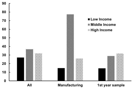
Figure 3.
Panel regression of products, estimating Equation (5). Percentage of countries with positive significant coefficient on technology: 1972–1988. The differences between income levels’ results are statistically significant in all three categories of All, Manufacturing, and 1st year sample.
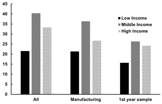
Figure 4.
Panel regression of products, estimating Equation (5). Percentage of countries with positive significant coefficient on technology: 1989–2001. The difference between income levels’ results are statistically significant in all three categories of All, Manufacturing, and 1st year sample.
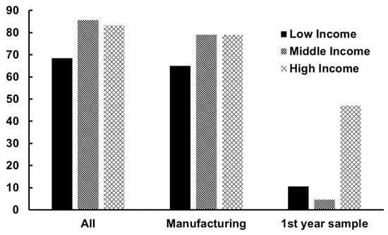
Figure 5.
Panel regression of products, estimating Equation (5). Percentage of countries with positive significant coefficients on capital: 1972–88. The differences between middle- and high-income countries in the All and Manufacturing categories, which are not statistically significant. All other differences are statistically significant in all categories.
Comparing Figure 1 and Figure 2 we see that the proportion of countries with positive significant coefficients has fallen over time and, in most cases, statistically significantly for skill accumulation. Interestingly, the one exception is middle income countries where the proportion has risen significantly when we consider products continuously exported throughout the entire sample period. The average magnitude of the positive significant coefficient (for detailed regression results, see Appendix B) has fallen to less than half in the 1989–2001 time period. The coefficient was 2.5 in 1989–2001 compared to 6 in 1972–1988. Since both skill levels and export unit values are log changes, the coefficient is an elasticity. So a 1% change in skill level will lead to a 6% increase in real unit value of exports in the earlier period and 2.5% in the latter period.
By contrast, in Figure 3 and Figure 4 we see that the proportion of countries with a positive coefficient for technology has remained steady, and the average significant positive coefficient—around 3.5 in both time periods—is also steady. There is a notable exception to this steadiness across time periods, and that is in the case of manufacturing products. Within manufacturing there is a significant and large shift where low-income countries rise and middle-income countries fall in the proportion of positive coefficients.
Figure 5 shows the proportion of countries with positive significant coefficients on capital accumulation. The proportions are the highest here compared to all graphs presented so far. Additionally, we find that the average magnitude of the positive significant coefficients on capital accumulation is the largest at 7. It is important to note that low-income countries have the lowest proportion of positive coefficients and there is no statistically significant difference among high- and middle-income countries in the proportion of positive coefficients. However, when products are limited to only those exported in the first year capital accumulation accelerates the growth of export quality (unit values) in the largest proportion of countries with high income. Among low- and middle-income countries, the proportion is statistically significantly smaller. There appears to be a core group of products which were exported throughout the sample period, where a large proportion of high-income countries have continued to enjoy rising unit values related to capital accumulation. On the other hand, middle- and low-income countries do not exhibit this feature. This finding is an interesting clue indicating that the nature of variety of goods exported by high-income versus other countries at the start of the sample period might be giving high-income countries a certain first mover advantage. It also provides an interesting question for future research that uses firm level data to disentangle the export baskets in these countries in the manner of Bernard et al. (2006).
Among other general patterns evident from the graphs is that middle-income countries have the highest proportion of positive coefficients. The graphs show where the differences among countries are statistically significant.
Product cycle theory offers some explanation for why middle-income countries might be expected to lead in the proportion of positive coefficients. On average, middle-income countries are in the middle of the unit value spectrum (Schott 2004) and have room to climb up the value ladder in their export products. Therefore, skill accumulation might manifest itself most clearly in increasing unit values of already exported products among middle-income countries. High-income countries are at the top of many of these ladders. When faced with competition, they might choose to abandon some of them (Schott 2002) and invest instead in developing new goods based on innovative technology. Low-income countries might also start exporting new products (new to them) in the natural process of growth, development, and technology diffusion from abroad (Grossman and Helpman 1991a and 1991b). Mukerji (2013) demonstrated the relatively more substantial growth of exports along the extensive margin in Global South countries than Global North countries. Therefore, for low- and high-income countries, increasing skill abundance might also manifest itself through the beginning of new product exports, rather than only climbing up the value ladder in existing exports.
6. Conclusions
6.1. Discussion
Among the results with respect to skill accumulation, both the results in country panel and product panel by individual countries seem to indicate diminishing importance as a source of trade competitiveness in the form of being able to command higher unit values in exports. In the earlier sample period, low-income countries were reaping the benefit of higher skills-related growth in unit values; however, over time, even this was eroded away. One potential explanation we have offered is that growing education levels in Global South countries in the latter time period have led to a more level playing field among countries in this regard and removed the edge in trade competitiveness that can be gained from skill improvement. We have also related worldwide skill accumulation to growing capacity for technology absorption by lower income countries, potentially shifting the focus of trade competition to the frontier of technology.
In the country panel regressions results (Section 5.1), capital accumulation has been associated with positive unit value of export growth, except in the case of low income countries. This country panel result is supported by the product panel results (Section 5.2) as the proportion of countries with positive coefficients with respect to capital accumulation is the lowest among low-income countries. The final piece of evidence that helps to tie these results together is that among products exported throughout the time sample by countries, high-income countries have the highest proportion of positive coefficients and other countries have remarkably low proportions. One explanation could be differences in the variety of goods that high-income countries sold at the start of the sample period compared to other countries. Firm level analysis could delve into this rich source of variation among countries in future studies.
Both country and product panels (in Section 5.1 and Section 5.2, respectively) indicate an overall positive impact of technology on unit values. However, there is a change in the latter time period in both types of analysis, which seems to indicate a notable aspect of the relationship of manufacturing to capital accumulation. In the country regression results, when the association with capital accumulation becomes negative, manufacturing is less negative than the general trend. In the product regressions, manufacturing sees the biggest shift between the two periods as low-income countries gain and middle-income countries lose in the proportion of positive coefficients. As mentioned in Section 5.1, the outcome of these shifts in manufacturing could be the potential reason behind the discord in multilateral international trade.
Our findings thus provide a potentially interesting explanation of the latest round of disputes centered around Global North countries’ reluctance to share technology. Examples are the disputes between China and the U.S. (Alper et al. 2019) and between Japan and South Korea (Jin and Takenaka 2019).
6.2. Overall Conclusions
This paper adds to the literature by utilizing product-level trade data to estimate the relation between export quality and factor accumulation. It accounts for the hitherto neglected endogeneity between these two variables. Adding to the extant literature dominated by cross-sectional studies, we ask whether factor accumulation is accompanied by improving export quality over time. The aim was to understand how countries at various stages of development compete in international markets over the long term. We found that, unlike cross-sectional studies, a positive association between export quality and factor accumulation is not a consistent pattern in panel data. The findings can be partly explained with the aid of the product cycle theory and price and technology-based competition. Moreover, the accelerated growth in high-level education across the world might play a role.
Our estimation based on considering the panel of products exported by each country separately indicates a steady and important role of technology in determining unit value of exports, and therefore trade competitiveness. Our estimation based on the panel of countries where all their exports are pooled together gives a more nuanced picture of how technology has benefited certain types of producers in trade more than others.
This paper attempts to contribute towards a more nuanced guide for policymakers by relating trade competitiveness to export characteristics. Understanding factor accumulation’s impact on a country’s trade and its competitors’ trade clarifies what a country can expect in international markets—thus providing a guide for trade policy based on economic fundamentals and not just political considerations.
Funding
This research was funded by the Research Matters Grant, Connecticut College.
Institutional Review Board Statement
Not applicable.
Informed Consent Statement
Not applicable.
Data Availability Statement
This data is publicly available. All data sources and links to the data are provided in Table 1.
Conflicts of Interest
The author declares no conflict of interest.
Appendix A
Table A1.
Countries included in regression presented in Table 4.
Table A1.
Countries included in regression presented in Table 4.
| Algeria |
| Argentina |
| Australia |
| Austria |
| Belize |
| Belgium |
| Benin |
| Bangladesh |
| Brazil |
| Burkina Faso |
| Burundi |
| Cameroon |
| Canada |
| Chile |
| China |
| Colombia |
| Congo |
| Costa Rica |
| Central African Republic |
| Denmark |
| Dominican Republic |
| Ecuador |
| Egypt |
| Fiji |
| Finland |
| France |
| Gabon |
| Gambia |
| Ghana |
| Greece |
| Guatemala |
| Guyana |
| Haiti |
| Honduras |
| Hong Kong |
| Hungary |
| Iceland |
| India |
| Indonesia |
| Iran |
| Ireland |
| Israel |
| Italy |
| Cote d’Ivoire |
| Jamaica |
| Japan |
| Jordan |
| Kenya |
| South Korea |
| Kuwait |
| Malawi |
| Malaysia |
| Mali |
| Malta |
| Mauritania |
| Mexico |
| Morocco |
| Mauritius |
| Nepal |
| Netherlands |
| Papua New Guinea |
| New Zealand |
| Nicaragua |
| Niger |
| Nigeria |
| Norway |
| Oman |
| Pakistan |
| Panama |
| Paraguay |
| Peru |
| Philippines |
| Portugal |
| Romania |
| Rwanda |
| El Salvador |
| Saudi Arabia |
| Senegal |
| Sierra Leone |
| Singapore |
| Spain |
| Sri Lanka |
| Sudan |
| Suriname |
| Sweden |
| Switzerland |
| Syria |
| South Africa |
| Thailand |
| Togo |
| Trinidad and Tobago |
| Tunisia |
| Turkey |
| United Kingdom |
| Uruguay |
| Venezuela |
| Democratic Republic of the Congo |
| Zambia |
| Zimbabwe |
Table A2.
Countries included in the regressions presented in Table 5.
Table A2.
Countries included in the regressions presented in Table 5.
| Argentina |
| Australia |
| Austria |
| Belgium |
| Bolivia |
| Canada |
| Chile |
| Colombia |
| Denmark |
| Dominican Republic |
| Ecuador |
| Finland |
| France |
| Germany |
| Greece |
| Guatemala |
| Honduras |
| Hong Kong |
| Iceland |
| India |
| Iran |
| Ireland |
| Israel |
| Italy |
| Cote d’Ivoire |
| Jamaica |
| Japan |
| Kenya |
| South Korea |
| Madagascar |
| Malawi |
| Mexico |
| Morocco |
| Mauritius |
| Nepal |
| Netherlands |
| New Zealand |
| Nigeria |
| Norway |
| Panama |
| Paraguay |
| Peru |
| Philippines |
| Portugal |
| Sierra Leone |
| Spain |
| Sri Lanka |
| Sweden |
| Switzerland |
| Syria |
| Thailand |
| Turkey |
| United Kingdom |
| Venezuela |
| Zambia |
| Zimbabwe |
Table A3.
Countries included in the regressions presented in Table 6.
Table A3.
Countries included in the regressions presented in Table 6.
| Albania |
| Algeria |
| Angola |
| United Arab Emirates |
| Argentina |
| Australia |
| Austria |
| Bahamas |
| Bahrain |
| Belize |
| Belgium |
| Benin |
| Bangladesh |
| Bolivia |
| Brazil |
| Bulgaria |
| Burkina Faso |
| Burundi |
| Cameroon |
| Canada |
| Chad |
| Chile |
| China |
| Colombia |
| Congo |
| Costa Rica |
| Cyprus |
| Central African Republic |
| Denmark |
| Dominican Republic |
| Ecuador |
| Egypt |
| Ethiopia |
| Fiji |
| Finland |
| France |
| Gabon |
| Gambia |
| Germany |
| Ghana |
| Greece |
| Guatemala |
| Guinea |
| Guyana |
| Guinea-Bissau |
| Haiti |
| Honduras |
| Hong Kong |
| Hungary |
| Iceland |
| India |
| Indonesia |
| Iran |
| Ireland |
| Israel |
| Italy |
| Cote d’Ivoire |
| Jamaica |
| Japan |
| Jordan |
| Kenya |
| Kiribati |
| South Korea |
| Kuwait |
| Laos |
| Liberia |
| Libya |
| Macau |
| Madagascar |
| Malawi |
| Malaysia |
| Mali |
| Malta |
| Mauritania |
| Mexico |
| Mongolia |
| Morocco |
| Mozambique |
| Mauritius |
| Nepal |
| Netherlands |
| New Caledonia |
| Papua New Guinea |
| New Zealand |
| Nicaragua |
| Niger |
| Nigeria |
| Norway |
| Oman |
| Pakistan |
| Panama |
| Paraguay |
| Peru |
| Philippines |
| Portugal |
| Romania |
| Rwanda |
| El Salvador |
| Samoa |
| Saudi Arabia |
| Senegal |
| Seychelles |
| Sierra Leone |
| Singapore |
| Spain |
| Sri Lanka |
| Saint Kitts and Nevis |
| Sudan |
| Suriname |
| Sweden |
| Switzerland |
| Syria |
| South Africa |
| Thailand |
| Togo |
| Trinidad and Tobago |
| Tunisia |
| Turkey |
| Uganda |
| United Kingdom |
| Uruguay |
| Venezuela |
| Democratic Republic of the Congo |
| Zambia |
| Zimbabwe |
Table A4.
Countries included in the regressions presented in Table 7.
Table A4.
Countries included in the regressions presented in Table 7.
| Algeria |
| Australia |
| Austria |
| Belize |
| Belgium |
| Benin |
| Brazil |
| Burkina Faso |
| Burundi |
| Cameroon |
| Canada |
| Chad |
| Chile |
| China |
| Colombia |
| Congo |
| Costa Rica |
| Central African Republic |
| Denmark |
| Dominican Republic |
| Ecuador |
| Egypt |
| Fiji |
| Finland |
| France |
| Gabon |
| Gambia |
| Georgia |
| Germany |
| Ghana |
| Greece |
| Guatemala |
| Guyana |
| Honduras |
| Hong Kong |
| Hungary |
| Iceland |
| India |
| Indonesia |
| Iran |
| Ireland |
| Israel |
| Italy |
| Cote d’Ivoire |
| Jamaica |
| Japan |
| Jordan |
| Kenya |
| South Korea |
| Kuwait |
| Latvia |
| Madagascar |
| Malawi |
| Malaysia |
| Mali |
| Malta |
| Mauritania |
| Mexico |
| Morocco |
| Mauritius |
| Nepal |
| Netherlands |
| Papua New Guinea |
| New Zealand |
| Nicaragua |
| Niger |
| Nigeria |
| Norway |
| Oman |
| Pakistan |
| Panama |
| Paraguay |
| Peru |
| Philippines |
| Portugal |
| Romania |
| El Salvador |
| Saudi Arabia |
| Senegal |
| Singapore |
| Spain |
| Sri Lanka |
| Sudan |
| Suriname |
| Sweden |
| Switzerland |
| Syria |
| South Africa |
| Thailand |
| Togo |
| Trinidad and Tobago |
| Tunisia |
| Turkey |
| United Kingdom |
| Uruguay |
| Venezuela |
| Democratic Republic of the Congo |
| Zambia |
Table A5.
Countries included in the regressions presented in Table 8.
Table A5.
Countries included in the regressions presented in Table 8.
| Albania |
| Algeria |
| Angola |
| United Arab Emirates |
| Argentina |
| Armenia |
| Australia |
| Austria |
| Azerbaijan |
| Bahamas |
| Bahrain |
| Belarus |
| Belize |
| Belgium |
| Benin |
| Bangladesh |
| Bolivia |
| Bosnia and Herzegovina |
| Brazil |
| Bulgaria |
| Burkina Faso |
| Burundi |
| Cambodia |
| Cameroon |
| Canada |
| Chad |
| Chile |
| China |
| Colombia |
| Congo |
| Costa Rica |
| Croatia |
| Cyprus |
| Czech Republic |
| Central African Republic |
| Denmark |
| Djibouti |
| Dominican Republic |
| Ecuador |
| Egypt |
| Equatorial Guinea |
| Estonia |
| Ethiopia |
| Fiji |
| Finland |
| France |
| Gabon |
| Gambia |
| Georgia |
| Germany |
| Ghana |
| Greece |
| Guatemala |
| Guinea |
| Guyana |
| Guinea-Bissau |
| Haiti |
| Honduras |
| Hong Kong |
| Hungary |
| Iceland |
| India |
| Indonesia |
| Iran |
| Ireland |
| Israel |
| Italy |
| Cote d’Ivoire |
| Jamaica |
| Japan |
| Jordan |
| Kazakhstan |
| Kenya |
| Kiribati |
| South Korea |
| Kuwait |
| Kyrgyz Republic |
| Laos |
| Latvia |
| Lebanon |
| Liberia |
| Lithuania |
| Macau |
| Macedonia |
| Madagascar |
| Malawi |
| Malaysia |
| Mali |
| Malta |
| Mauritania |
| Mexico |
| Moldova |
| Mongolia |
| Morocco |
| Mozambique |
| Mauritius |
| Nepal |
| Netherlands |
| New Caledonia |
| Papua New Guinea |
| New Zealand |
| Nicaragua |
| Niger |
| Nigeria |
| Norway |
| Oman |
| Pakistan |
| Panama |
| Paraguay |
| Peru |
| Philippines |
| Poland |
| Portugal |
| Romania |
| Russia |
| Rwanda |
| El Salvador |
| Samoa |
| Saudi Arabia |
| Senegal |
| Seychelles |
| Sierra Leone |
| Singapore |
| Slovak Republic |
| Slovenia |
| Spain |
| Sri Lanka |
| Saint Kitts and Nevis |
| Sudan |
| Suriname |
| Sweden |
| Switzerland |
| Syria |
| South Africa |
| Tajikistan |
| Tanzania |
| Thailand |
| Togo |
| Trinidad and Tobago |
| Tunisia |
| Turkey |
| Turkmenistan |
| Uganda |
| United Kingdom |
| Ukraine |
| Uruguay |
| Uzbekistan |
| Venezuela |
| Vietnam |
| Yemen |
| Yugoslavia |
| Democratic Republic of the Congo |
| Zambia |
| Zimbabwe |
Appendix B
Regressions include product dummies and interaction of year and product-SITC dummies.
Regression run:
| Measures Technology Years: 1989–2001 | ||
|---|---|---|
| Low-Income Countries | ||
| Estimate | t-Stat. | |
| TAJIKISTAN | 3.137 | 1.654 * |
| UGANDA | 7.993 | 2.248 ** |
| KYRGYZSTAN | −6.279 | −4.754 |
| IVORY COAST | 3.005 | 3.221 *** |
| GEORGIA | 1.010 | 0.560 |
| EQUATORIAL GUINEA | 0.545 | 0.752 |
| AZERBAIJAN | −0.439 | −0.541 |
| TOGO | −1.690 | −1.780 |
| BANGLADESH | −0.206 | −0.220 |
| INDIA | −0.921 | −3.220 |
| CHAD | 1.184 | 0.198 |
| SENEGAL | −4.440 | −2.465 |
| ARMENIA | 10.651 | 7.301 *** |
| BURUNDI | 0.511 | 0.114 |
| CAMEROON | 0.961 | 0.966 |
| KIRIBATI | −1.546 | −0.912 |
| NEPAL | −2.289 | −3.132 |
| MALI | −6.349 | −2.743 |
| SRI LANKA | −0.856 | −1.171 |
| PAKISTAN | −1.032 | −2.605 |
| UKRAINE | −0.069 | −0.242 |
| SUDAN | −1.141 | −0.769 |
| RWANDA | −0.557 | −0.995 |
| NICARAGUA | −3.566 | −4.395 |
| BENIN | 36.668 | 1.853 * |
| GUYANA | 2.828 | 5.278 *** |
| GHANA | −16.716 | −4.094 |
| TURKMENISTAN | −3.634 | −4.408 |
| TANZANIA | −4.703 | −1.614 |
| INDONESIA | 0.407 | 4.946 *** |
| MAURITIAN | −3.654 | −0.350 |
| YEMEN | −1.023 | −0.341 |
| PHILIPPINES | 0.446 | 1.710 * |
| MOLDOVA | −1.711 | −3.705 |
| MALAWI | 1.850 | 2.730 *** |
| KENYA | −4.017 | −2.818 |
| ZAIRE | 0.722 | 0.575 |
| LIBERIA | −0.654 | −2.102 |
| HONDURA | −1.154 | −3.227 |
| LAOS | −31.988 | −6.637 |
| GUINEA | −0.067 | −0.014 |
| CENTRAL AFRICA | 0.582 | 0.110 |
| ZIMBABWE | −1.276 | −3.516 |
| ALBANIA | −2.819 | −5.175 |
| UZBEKISTAN | −26.741 | −8.080 |
| NIGER | 9.397 | 2.494 *** |
| BOLIVIA | −1.033 | −0.811 |
| CHINA | 0.616 | 4.678 *** |
| SIERRA LEONE | 2.265 | 2.855 *** |
| GUINEA BISSAU | −2.078 | −1.262 |
| MOZAMBIQUE | −2.163 | −0.921 |
| ETHIOPIA | −2.280 | −4.120 |
| CAMBODIA | 1.144 | 1.523 |
| NIGERIA | 3.264 | 2.362 *** |
| BURKINA | −5.359 | −1.542 |
| NEW GUINEA | 2.853 | 2.300 *** |
| MONGOLA | −4.917 | −7.411 |
| SYRIA | −0.363 | −0.620 |
| HAITI | −0.096 | −0.422 |
| ZAMBIA | −1.077 | −0.447 |
| BOSNIA AND HERZEGOVINA | 1.047 | 3.081 *** |
| GAMBIA | −8.251 | −1.947 |
| VIETNAM | 4.081 | 3.953 *** |
| ANGOLA | 6.830 | 5.417 *** |
| MADAGASCAR | −11.858 | −7.857 |
| Middle-Income Countries | ||
| BRAZIL | 0.323 | 1.463 |
| GABON | −9.438 | −6.384 |
| COSTA RICA | −1.763 | −5.445 |
| PANAMA | 1.745 | 2.819 *** |
| VENEZUELA | 0.614 | 2.547 *** |
| POLAND | −3.548 | −10.718 |
| URUGUAY | −0.151 | −0.361 |
| ECUADOR | 1.386 | 4.768 *** |
| PARAGUAY | −3.921 | −2.411 *** |
| CZECHOSLOVAKIA | −0.185 | −0.625 |
| SOUTH AFRICA | 5.386 | 9.218 *** |
| ARGENTINA | 0.585 | 3.053 *** |
| LITHUANIA | 1.398 | 3.709 *** |
| MOROCCO | −0.610 | −2.911 *** |
| GUATEMALA | −0.113 | −0.115 |
| FIJI | 2.160 | 3.416 *** |
| DOMINICAN REPUBLIC | −2.225 | −9.399 *** |
| BELIZE | −3.114 | −6.589 *** |
| SEYCHELLE | −10.074 | −1.507 |
| SLOVAKIA | 5.252 | 3.839 *** |
| PORTUGAL | −0.322 | −0.913 |
| TURKEY | 0.576 | 4.324 *** |
| CHILE | 2.696 | 9.243 *** |
| LEBANON | −1.660 | −8.249 *** |
| TUNISIA | −2.783 | −2.951 *** |
| BULGARIA | −1.025 | −3.455 *** |
| MALAYSIA | 0.476 | 3.438 *** |
| MAURITIUS | 7.729 | 3.191 *** |
| IRAN | −7.755 | −1.318 |
| CONGO | −1.185 | −0.753 |
| LATVIA | 0.588 | 0.417 |
| MACEDONIA | 2.067 | 3.927 *** |
| CROATIA | −2.418 | −8.964 *** |
| MEXICO | −0.028 | −0.270 |
| GREECE | −0.531 | −0.955 |
| TRINIDAD | −1.899 | −2.995 *** |
| SAINT KITTS AND NEVIS | 2.790 | 3.228 *** |
| HUNGARY | −4.466 | −17.811 *** |
| RUSSIA | −0.297 | −1.599 |
| KAZAKHSTAN | −0.681 | −1.507 |
| SOUTH KOREA | 1.014 | 11.500 *** |
| SLOVENIA | −6.060 | −2.707 *** |
| BELARUS | −0.653 | −1.979 *** |
| ALGERIA | −6.463 | −2.331 *** |
| EGYPT | −4.104 | −4.458 *** |
| JORDAN | 2.059 | 3.356 *** |
| THAILAND | 1.112 | 13.954 *** |
| PERU | 1.244 | 6.336 *** |
| MALTA | 2.911 | 0.780 |
| ROMANIA | −0.494 | −2.304 *** |
| COLOMBIA | 1.455 | 5.813 *** |
| SALVADOR | 4.512 | 10.113 *** |
| JAMAICA | 1.477 | 2.193 ** |
| SURINAME | 6.884 | 4.226 *** |
| ESTONIA | −0.339 | −0.387 |
| SAMOA | −3.933 | −1.996 ** |
| OMAN | 2.223 | 4.727 *** |
| High-Income Countries | ||
| SPAIN | 0.366 | 0.879 |
| MACAU | 2.683 | 15.907 *** |
| ARAB EMPIRE | −1.109 | −3.323 *** |
| ISRAEL | 1.501 | 2.917 *** |
| GERMANY | 1.810 | 7.841 *** |
| ICELAND | −7.411 | −10.729 *** |
| KUWAIT | 6.246 | 4.571 *** |
| BELGIUM-LUXEMBOURG | −0.618 | −1.286 |
| AUSTRIA | 0.198 | 0.342 |
| SINGAPORE | −0.219 | −0.894 |
| ITALY | 2.622 | 7.668 *** |
| NEW ZEALAND | −4.143 | −8.708 *** |
| SAUDI ARABIA | 4.067 | 4.402 *** |
| NETHERLANDS | −4.055 | −6.667 *** |
| CYPRUS | −1.369 | −1.733 * |
| JAPAN | 1.301 | 6.291 *** |
| IRELAND | −0.838 | −2.209 ** |
| HONGKONG | −0.107 | −0.826 |
| UNITED KINGDOM | −1.283 | −4.850 *** |
| DENMARK | −0.334 | −0.530 |
| AUSTRALIA | 0.468 | 4.929 *** |
| NORWAY | 1.533 | 1.645 * |
| SWITZERLAND | −1.372 | −3.805 *** |
| BAHAMAS | −10.749 | −7.526 *** |
| NEW CATALONIA | −5.074 | −2.215 ** |
| CANADA | −1.724 | −13.499 *** |
| BAHRAIN | 2.203 | 3.620 *** |
| FRANCE | 0.902 | 2.800 *** |
| FINLAND | −0.658 | −2.202 ** |
| SWEDEN | −1.875 | −6.017 *** |
* significant at 10%; ** significant at 5%; *** significant at 1%.
| Measures Technology Years: 1972–1988 | ||
|---|---|---|
| Low-Income Countries | ||
| Estimate | t-Stat. | |
| Togo | −0.117 | −0.019 |
| Bangladesh | −3.400 | −2.650 *** |
| Nepal | −1.009 | −1.198 |
| Zambia | −16.619 | −3.549 *** |
| Congo, Dem. Rep. | −2.595 | −1.169 |
| Mozambique | 3.656 | 1.640 |
| Kiribati | −4.474 | −4.093 *** |
| Gambia, The | 6.193 | 1.370 |
| Pakistan | −5.762 | −10.129 *** |
| China | −1.720 | −9.088 *** |
| Morocco | −0.811 | −1.841 * |
| Sri Lanka | 0.084 | 0.226 |
| Central African Republic | 1.045 | 0.117 |
| Cote d’Ivoire | −0.574 | −0.490 |
| Rwanda | 4.417 | 0.519 |
| Mali | 0.617 | 0.404 |
| Sudan | 2.800 | 0.704 |
| Senegal | −1.073 | −0.355 |
| Malawi | −5.105 | −0.766 |
| Egypt, Arab Rep. | −2.920 | −3.812 *** |
| Papua New Guinea | −0.473 | −0.055 |
| Benin | 4.855 | 0.713 |
| Guinea-Bissau | 11.400 | 1.526 |
| Uganda | −6.952 | −0.625 |
| Sierra Leone | 18.089 | 4.329 *** |
| Kenya | −1.677 | −0.926 |
| Guyana | 0.732 | 0.710 |
| Liberia | 4.168 | 0.810 |
| Haiti | 1.677 | 5.362 *** |
| Ethiopia | −1.677 | −1.209 |
| Nicaragua | 1.630 | 3.995 *** |
| Honduras | 3.714 | 4.379 *** |
| Thailand | −0.826 | −2.472 *** |
| Indonesia | −0.039 | −0.070 |
| India | −0.776 | −4.345 *** |
| Congo, Rep. | −3.428 | −1.974 ** |
| Niger | 8.745 | 5.232 *** |
| Zimbabwe | 7.038 | 3.792 *** |
| Mauritania | 8.428 | 1.295 |
| Madagascar | −0.212 | −0.073 |
| Syrian Arab Republic | 1.248 | 1.525 |
| Nigeria | −2.851 | −2.392 *** |
| Cameroon | −2.216 | −1.556 |
| Burkina Faso | 3.242 | 1.415 |
| Philippines | −0.552 | −3.613 *** |
| Bolivia | 2.680 | 2.887 *** |
| Ghana | −4.258 | −3.621 *** |
| Middle-Income Countries | ||
| Mexico | 2.970 | 19.865 *** |
| Brazil | 1.617 | 10.246 *** |
| Malta | 1.448 | 1.275 |
| Malaysia | 2.020 | 6.155 *** |
| Samoa | 0.047 | 0.010 |
| Peru | 0.769 | 4.132 *** |
| Panama | 0.301 | 0.910 |
| Belize | 5.146 | 4.834 *** |
| Venezuela, RB | 3.804 | 6.073 *** |
| Turkey | −2.903 | −6.094 *** |
| Guatemala | −1.067 | −2.034 ** |
| Portugal | −1.408 | −6.285 *** |
| Trinidad and Tobago | −1.084 | −1.045 |
| Greece | −1.903 | −5.286 *** |
| Costa Rica | −0.638 | −1.939 * |
| Dominican Republic | 0.530 | 1.469 |
| Uruguay | −2.441 | −6.626 *** |
| Suriname | −1.126 | −0.571 |
| Paraguay | −5.956 | −5.957 *** |
| Italy | 1.364 | 6.331 *** |
| Chile | −1.927 | −5.288 *** |
| Oman | −5.677 | −2.577 *** |
| Seychelles | −10.661 | −2.791 *** |
| Bulgaria | 8.717 | 4.520 *** |
| Ecuador | −1.300 | −2.413 *** |
| Colombia | 0.819 | 1.316 |
| Cyprus | 1.924 | 1.934 *** |
| Iran, Islamic Rep. | 0.289 | 0.469 |
| Gabon | −1.336 | −0.606 |
| Korea, Rep. | −1.873 | −11.940 *** |
| El Salvador | −0.316 | −0.866 |
| Jordan | −2.751 | −1.022 |
| Algeria | −13.159 | −1.843 ** |
| Spain | −0.611 | −1.955 ** |
| Fiji | −0.425 | −0.406 |
| Tunisia | −7.002 | −5.201 *** |
| Hungary | −0.920 | −1.332 |
| St. Kitts and Nevis | −0.974 | −1.145 |
| Romania | −3.123 | −5.877 *** |
| South Africa | 1.529 | 3.075 *** |
| Libya | 4.066 | 0.682 |
| Argentina | 1.125 | 4.795 *** |
| Jamaica | −2.253 | −4.558 *** |
| Mauritius | 15.443 | 9.374 *** |
| High-Income Countries | ||
| Netherlands | 2.711 | 6.145 *** |
| Sweden | −0.441 | −0.881 |
| Israel | −0.744 | −1.538 |
| Bahamas, The | −0.230 | −0.412 |
| Finland | −4.717 | −7.088 |
| France | 0.967 | 2.662 *** |
| Kuwait | −1.415 | −1.375 |
| Germany | 1.803 | 7.817 *** |
| Japan | −0.368 | −2.265 ** |
| Hong Kong, China | −2.343 | −22.567 *** |
| Saudi Arabia | 1.640 | 1.565 |
| Bahrain | −7.038 | −4.690 *** |
| Austria | 2.810 | 5.923 *** |
| United Arab Emirates | −2.022 | −2.610 *** |
| New Zealand | −4.124 | −5.506 *** |
| Singapore | −0.734 | −2.510 *** |
| Belgium | 2.096 | 6.003 *** |
| Iceland | 0.150 | 0.155 |
| Switzerland | −2.139 | −8.795 *** |
| Denmark | −2.325 | −5.757 *** |
| Ireland | 1.972 | 3.971 *** |
| Macao, China | −0.680 | −2.402 *** |
| New Caledonia | −1.332 | −0.991 |
| Australia | −3.980 | −7.042 *** |
| Canada | 0.314 | 1.581 |
| United Kingdom | −2.804 | −15.034 *** |
| Norway | 2.447 | 4.040 *** |
* significant at 10%; ** significant at 5%; *** significant at 1%.
| Measures Skill Years: 1989–2001 | ||
|---|---|---|
| Low-Income Countries | ||
| Estimate | t-Stat. | |
| FIJI | 2.560 | 1.723 * |
| KUWAIT | −0.409 | −2.361 *** |
| INDIA | −0.584 | −2.198 ** |
| SYRIA | −7.679 | −2.250 ** |
| CHAD | 2.152 | 0.297 |
| NIGER | −14.726 | −3.327 *** |
| SRI LANKA | −3.187 | −3.779 *** |
| MALI | 6.471 | 2.802 *** |
| NEW GUINEA | 6.661 | 3.069 *** |
| MADAGASCAR | 1.412 | 0.928 |
| KENYA | −0.201 | −0.461 |
| BENIN | −25.948 | −4.040 *** |
| GUYANA | −4.814 | −4.401 *** |
| PHILIPPINES | −1.369 | −2.302 *** |
| NEPAL | 0.427 | 0.662 |
| CHINA | 0.229 | 1.307 |
| MALAWI | 2.154 | 2.469 *** |
| HONDURA | −14.604 | −2.364 *** |
| TOGO | −4.458 | −1.950 * |
| CAMEROON | −9.174 | −7.596 *** |
| NICARAGUA | 1.818 | 3.655 *** |
| SENEGAL | −0.080 | −0.037 |
| ZAMBIA | −60.834 | −2.868 *** |
| INDONESIA | 0.865 | 4.948 *** |
| ZIMBABWE | −0.416 | −0.706 |
| NIGERIA | 2.672 | 1.735 *** |
| GAMBIA | 2.105 | 1.564 |
| BURUNDI | −14.180 | −4.579 *** |
| IVORY COAST | 0.422 | 0.267 |
| Middle-Income Countries | ||
| ROMANIA | −4.096 | −8.219 *** |
| TURKEY | −1.588 | −2.970 *** |
| BELIZE | −1.000 | −1.548 |
| PANAMA | −11.199 | −6.423 *** |
| CHILE | 0.368 | 1.261 |
| SURINAM | −4.395 | −4.120 *** |
| THAILAND | 1.146 | 7.241 *** |
| SOUTH AFRICA | 11.569 | 6.419 *** |
| IRAN | 11.814 | 0.913 |
| VENEZUELA | 1.275 | 4.128 *** |
| OMAN | 3.379 | 12.864 *** |
| EGYPT | 1.111 | 1.805 * |
| TUNISIA | −3.133 | −4.723 *** |
| ECUADOR | 1.646 | 7.344 *** |
| CONGO | 0.967 | 0.202 |
| HUNGARY | −1.427 | −3.532 *** |
| DOMINICAN REPUBLIC | −0.574 | −1.231 |
| MOROCCO | 2.636 | 3.374 *** |
| PORTUGAL | 1.121 | 7.033 *** |
| COLOMBIA | 0.750 | 3.384 *** |
| URUGUAY | −1.860 | −2.492 *** |
| GUATEMALA | 0.376 | 0.926 |
| PERU | 0.532 | 1.108 |
| LATVIA | 7.895 | 0.555 |
| GABON | 1.997 | 0.701 |
| MEXICO | −2.488 | −10.965 *** |
| SOUTH KOREA | 0.257 | 1.030 |
| ALGERIA | −20.017 | −3.252 *** |
| MALAYSIA | −1.636 | −5.721 *** |
| PARAGUAY | −2.606 | −2.940 *** |
| JAMAICA | 2.742 | 1.061 |
| BRAZIL | −0.459 | −1.453 |
| JORDAN | 2.556 | 1.368 |
| GREECE | 2.993 | 3.888 *** |
| MAURITIAN | −0.922 | −0.635 |
| MALTA | 4.069 | 2.390 *** |
| SALVADOR | −0.502 | −2.552 *** |
| COSTA RICA | −0.161 | −0.248 |
| TRINIDAD | −0.445 | −0.233 |
| High-Income Countries | ||
| JAPAN | 0.608 | 2.360 *** |
| NORWAY | −0.609 | −2.190 ** |
| AUSTRIA | 2.498 | 2.435 *** |
| SWEDEN | 0.006 | 0.059 |
| ICELAND | −8.240 | −6.706 *** |
| HONGKONG | 0.172 | 0.949 |
| AUSTRALIA | 0.129 | 1.939 * |
| IRELAND | 1.067 | 2.104 ** |
| ITALY | −3.152 | −9.361 *** |
| BELGIUM-LUXEMBOURG | 0.062 | 0.815 |
| GERMANY | 0.586 | 2.446 *** |
| SAUDI ARABIA | −9.472 | −4.218 |
| SPAIN | −0.361 | −0.987 |
| SINGAPORE | 1.501 | 3.801 *** |
| FRANCE | −0.805 | −4.122 *** |
| FINLAND | −2.229 | −3.417 *** |
| SWITZERLAND | 1.366 | 1.416 |
| DENMARK | −3.474 | −3.128 *** |
| CANADA | 3.869 | 6.555 *** |
| NETHERLANDS | −0.123 | −0.796 |
| UNITED KINGDOM | 0.076 | 1.890 *** |
| NEW ZEALAND | −0.936 | −2.071 ** |
| ISRAEL | 0.660 | 1.046 |
* significant at 10%; ** significant at 5%; *** significant at 1%.
| Measures Skill Years: 1972–1988 | ||
|---|---|---|
| Low-Income Countries | ||
| Estimate | t-Stat. | |
| BARBADOS | −5.158 | −2.732 *** |
| THAILAND | 6.209 | 12.316 *** |
| PHILIPPINES | −1.468 | −5.922 *** |
| IVORY COAST | −4.696 | −2.681 *** |
| MALI | 0.192 | 0.097 |
| GHANA | 1.479 | 0.430 |
| ZAMBIA | −7.719 | −1.368 |
| SUDAN | −27.575 | −3.809 *** |
| EGYPT | 14.924 | 10.351 *** |
| BURKINA | −2.204 | −3.160 *** |
| KENYA | 4.153 | 4.389 *** |
| SENEGAL | −2.725 | −0.660 |
| CENTRAL AFRICA | −9.965 | −2.963 *** |
| GUYANA | −3.302 | −3.297 *** |
| NIGER | −8.979 | −2.486 *** |
| NEW GUINEA | −13.545 | −1.156 |
| NIGERIA | 1.165 | 2.170 ** |
| NEPAL | −2.759 | −3.989 *** |
| SRI_LKA | −1.085 | −1.703 * |
| MAURITIUS | −1.774 | −0.097 |
| BANGLADESH | −0.806 | −3.033 *** |
| HAITI | −0.307 | −2.170 ** |
| HONDURA | 5.325 | 7.542 *** |
| SYRIA | −3.621 | −0.818 |
| INDIA | 0.730 | 1.585 |
| TOGO | −10.685 | −3.091 *** |
| CAMEROON | 8.878 | 3.348 *** |
| INDONESIA | −0.651 | −2.115 ** |
| ZAIRE | 1.056 | 0.726 |
| MALAWI | 2.215 | 0.537 |
| MOROCCO | 0.133 | 0.168 |
| SIERRA LEONE | 8.621 | 2.886 *** |
| ZIMBABWE | 1.830 | 4.071 *** |
| CHINA | −1.441 | −20.933 *** |
| Middle-Income Countries | ||
| TURKEY | 0.115 | 0.086 |
| ARGENTINA | −2.033 | −4.920 *** |
| MAURITIAN | 7.030 | 6.779 *** |
| VENEZUELA | 1.340 | 9.814 *** |
| SPAIN | 0.193 | 0.611 |
| JORDAN | 2.775 | 0.458 |
| OMAN | 4.805 | 0.686 |
| JAMAICA | −1.958 | −2.675 *** |
| MEXICO | −0.285 | −0.950 |
| PARAGUAY | 18.900 | 10.715 *** |
| BRAZIL | 0.420 | 1.623 |
| GUATEMALA | −6.798 | −8.810 *** |
| SOUTH KOREA | 1.217 | 4.632 *** |
| URUGUAY | −6.334 | −4.813 *** |
| IRAN | 5.172 | 2.584 *** |
| PANAMA | −12.963 | −5.108 *** |
| COLOMBIA | 0.126 | 0.714 |
| FIJI | −3.160 | −0.912 |
| TRINIDAD | 12.753 | 4.437 *** |
| GABON | 2.759 | 0.560 |
| PORTUGAL | 0.205 | 1.754 * |
| ROMANIA | 1.343 | 4.891 *** |
| SURINAM | −1.160 | −0.499 |
| BELIZE | −8.140 | −3.610 *** |
| SALVADOR | 3.121 | 6.969 *** |
| HUNGARY | −0.673 | −0.925 |
| ALGERIA | −7.270 | −1.357 |
| MALTA | 5.311 | 2.436 *** |
| MALAYSIA | −3.372 | −6.982 *** |
| PERU | −1.955 | −1.578 |
| GREECE | 1.594 | 2.159 ** |
| NICARAGUA | −3.205 | −1.457 |
| CHILE | −3.450 | −4.963 *** |
| CONGO | 6.733 | 2.119 ** |
| COSTA RICA | −5.927 | −8.132 *** |
| DOMINICAN REPUBLIC | 0.896 | 4.832 *** |
| TUNISIA | −7.520 | −5.496 *** |
| ECUADOR | 1.134 | 1.599 |
| High-Income Countries | ||
| SAUDI ARABIA | 2.131 | 0.952 |
| DENMARK | −5.904 | −4.700 *** |
| ITALY | −5.249 | −10.844 *** |
| NETHERLANDS | 0.375 | 2.159 ** |
| UNITED KINGDOM | 6.147 | 7.352 *** |
| SWEDEN | 0.593 | 1.363 |
| ISRAEL | −3.353 | −4.298 *** |
| ICELAND | 2.836 | 0.912 |
| HONGKONG | −18.827 | −21.670 *** |
| NORWAY | 0.955 | 0.682 |
| AUSTRIA | −0.064 | −0.476 |
| KUWAIT | −2.701 | −0.332 |
| BELGIUM−LUXEMBOURG | 1.290 | 2.439 *** |
| FINLAND | −4.118 | −3.744 *** |
| IRELAND | 20.754 | 10.133 *** |
| AUSTRAL | −0.187 | −0.780 |
| NEW ZEALAND | 2.743 | 1.830 * |
| FRANCE | 7.980 | 5.113 *** |
| SINGAPORE | −0.873 | −3.717 *** |
| CANADA | −4.252 | −14.135 *** |
| JAPAN | −0.432 | −0.986 |
| SWITZERLAND | 9.509 | 4.546 *** |
* significant at 10%; ** significant at 5%; *** significant at 1%.
| Measures Capital Years: 1972–1988 | ||
|---|---|---|
| Low-Income Countries | ||
| Estimate | t-Stat. | |
| Name | Yhat_Estimate | Yhat_Tstat |
| POLAND | 1.700 | 0.817 |
| YUGOSLAVIA | 8.723 | 12.401 *** |
| IRAN | 4.732 | 5.710 *** |
| TAIWAN | 3.931 | 19.311 *** |
| SYRIA | −6.035 | −3.295 *** |
| KENYA | 5.905 | 4.222 *** |
| PHILIPPINES | 3.558 | 10.298 *** |
| HONDURA | 3.675 | 6.812 *** |
| NEPAL | 0.463 | 0.192 |
| INDIA | 14.008 | 14.399 *** |
| IVORY COAST | 3.564 | 2.944 *** |
| SRI LANKA | −0.646 | −0.429 |
| BOLIVIA | 2.689 | 3.628 *** |
| MALAWI | −5.803 | −0.886 |
| SIERRA LEONE | −3.428 | −0.354 |
| NIGERIA | 5.517 | 4.487 *** |
| THAILAND | 3.413 | 6.999 *** |
| ZIMBABWE | 9.990 | 4.000 *** |
| MOROCCO | 1.543 | 3.042 *** |
| ZAMBIA | 5.651 | 0.944 |
| Middle-Income Countries | ||
| PARAGUAY | −0.497 | −0.651 |
| MAURITIUS | 3.935 | 7.871 *** |
| CHILE | −1.206 | −2.247 ** |
| GUATEMALA | 3.557 | 7.174 *** |
| PORTUGAL | 3.645 | 10.267 *** |
| ITALY | 11.851 | 31.457 *** |
| SPAIN | 3.546 | 10.095 *** |
| PANAMA | 2.893 | 2.310 *** |
| GREECE | 11.556 | 17.877 *** |
| SOUTH KOREA | 4.781 | 19.208 *** |
| TURKEY | 1.893 | 2.433 *** |
| COLOMBIA | 14.066 | 14.470 *** |
| PERU | 0.310 | 0.628 |
| VENEZUELA | 4.560 | 4.840 *** |
| ECUADOR | 0.846 | 0.965 |
| JAMAICA | 5.064 | 6.171 *** |
| ARGENTINA | 4.451 | 6.965 *** |
| MEXICO | 0.615 | 2.853 *** |
| DOMINICAN REPUBLIC | 7.110 | 15.766 *** |
| High-Income Countries | ||
| BELGIUM−LUXEMBOURG | 13.003 | 25.055 *** |
| GERMANY | 17.464 | 42.090 *** |
| SWEDEN | 2.694 | 6.127 *** |
| NORWAY | 1.395 | 1.432 |
| JAPAN | 7.794 | 36.236 *** |
| SWITZERLAND | 6.746 | 13.022 *** |
| UNITED KINGDOM | 8.121 | 19.872 *** |
| NETHERLANDS | 12.087 | 20.589 *** |
| DENMARK | 4.745 | 6.707 *** |
| HONGKONG | 1.010 | 7.751 *** |
| NEW ZEALAND | 0.095 | 0.066 |
| ISRAEL | 4.844 | 8.242 *** |
| FRANCE | 11.056 | 33.117 *** |
| CANADA | −11.501 | −25.380 *** |
| ICELAND | −1.827 | −0.925 |
| FINLAND | 17.792 | 15.444 *** |
| AUSTRIA | 13.280 | 21.715 *** |
| AUSTRALIA | 21.066 | 7.541 *** |
| IRELAND | 10.529 | 16.306 *** |
* significant at 10%; ** significant at 5%; *** significant at 1%.
Appendix C
The source of the information presented here is the WITS trade database of the World Bank. https://wits.worldbank.org/countrystats.aspx (accessed on 5 August 2021).
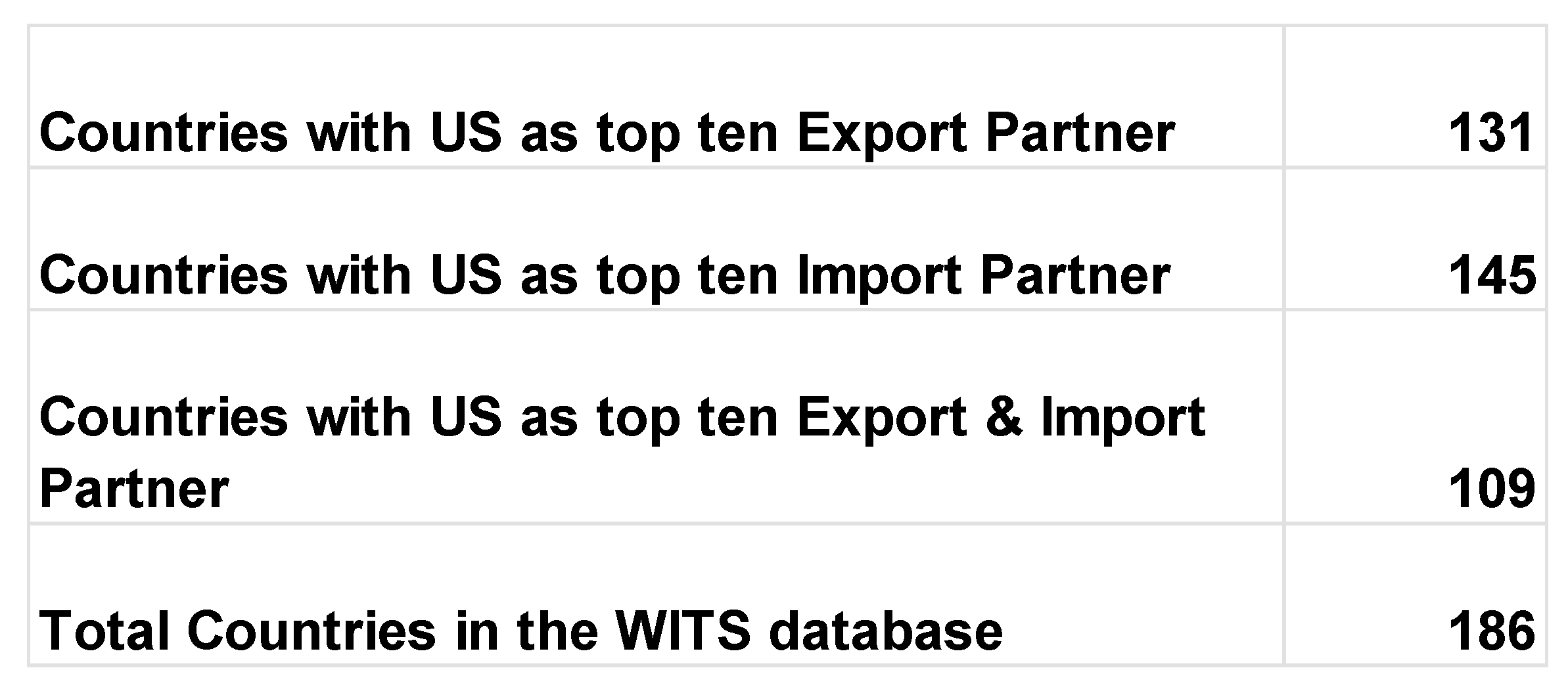
Below is the list of top ten countries that are export partners of each country in the World bank WITS trade database in 2020:
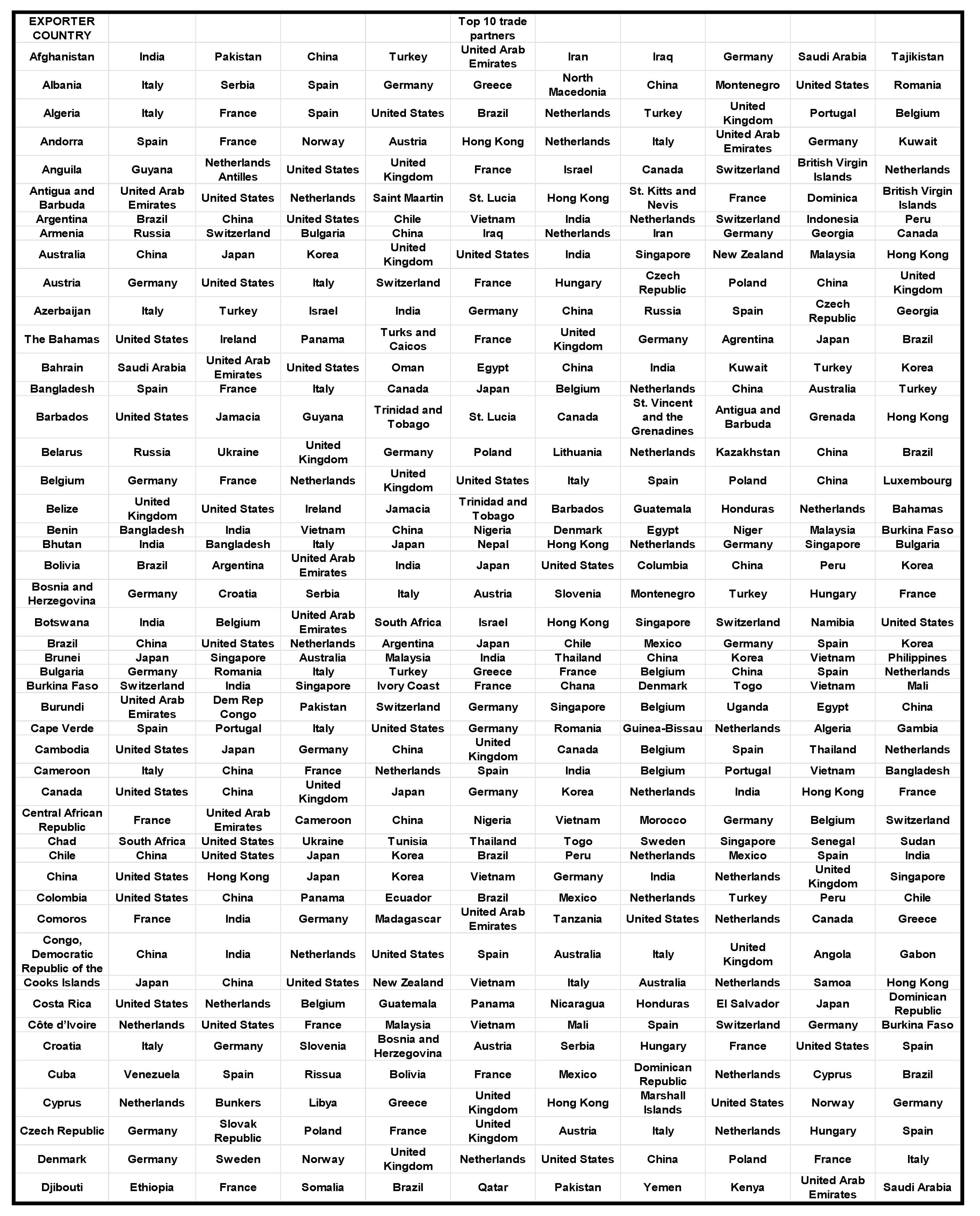
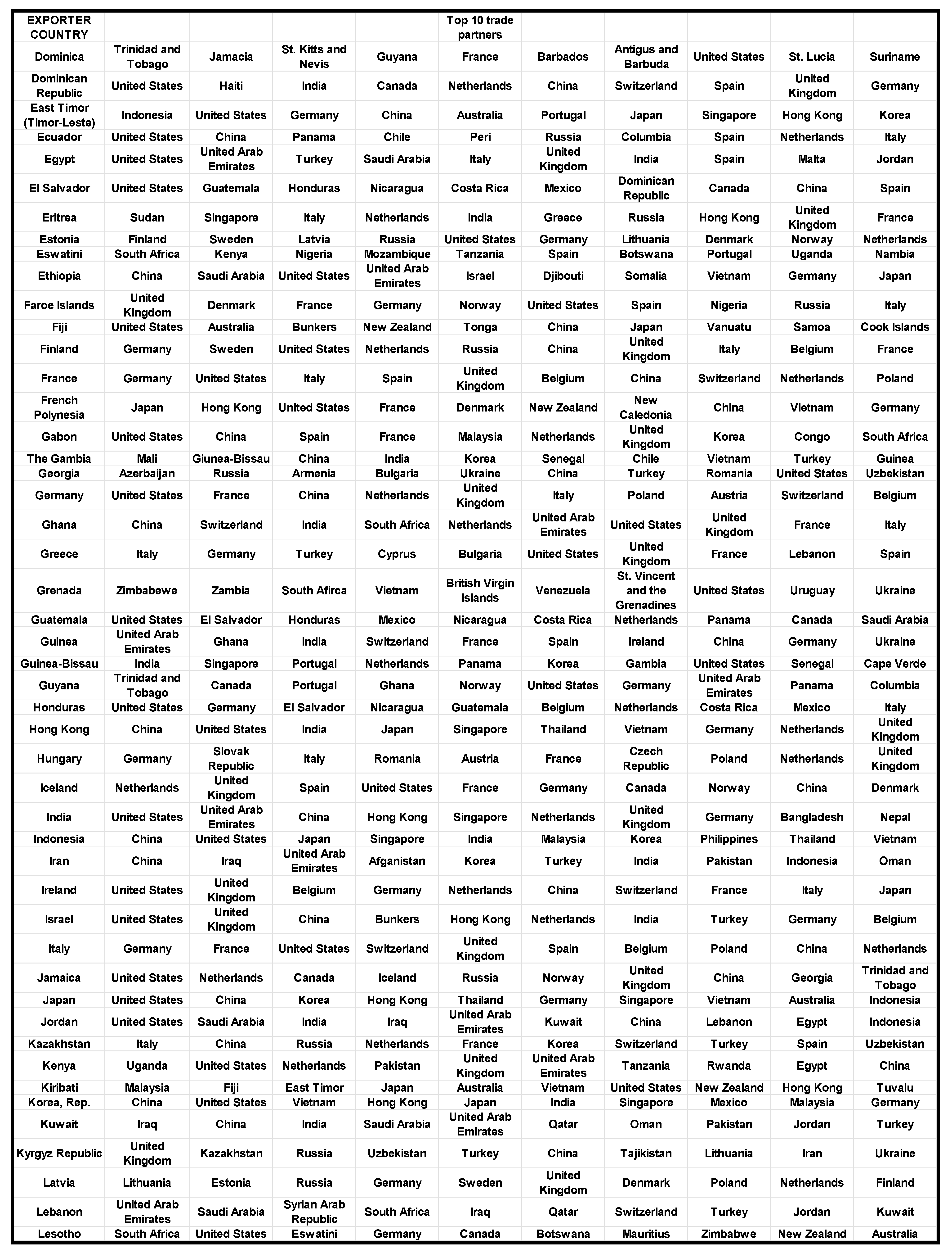
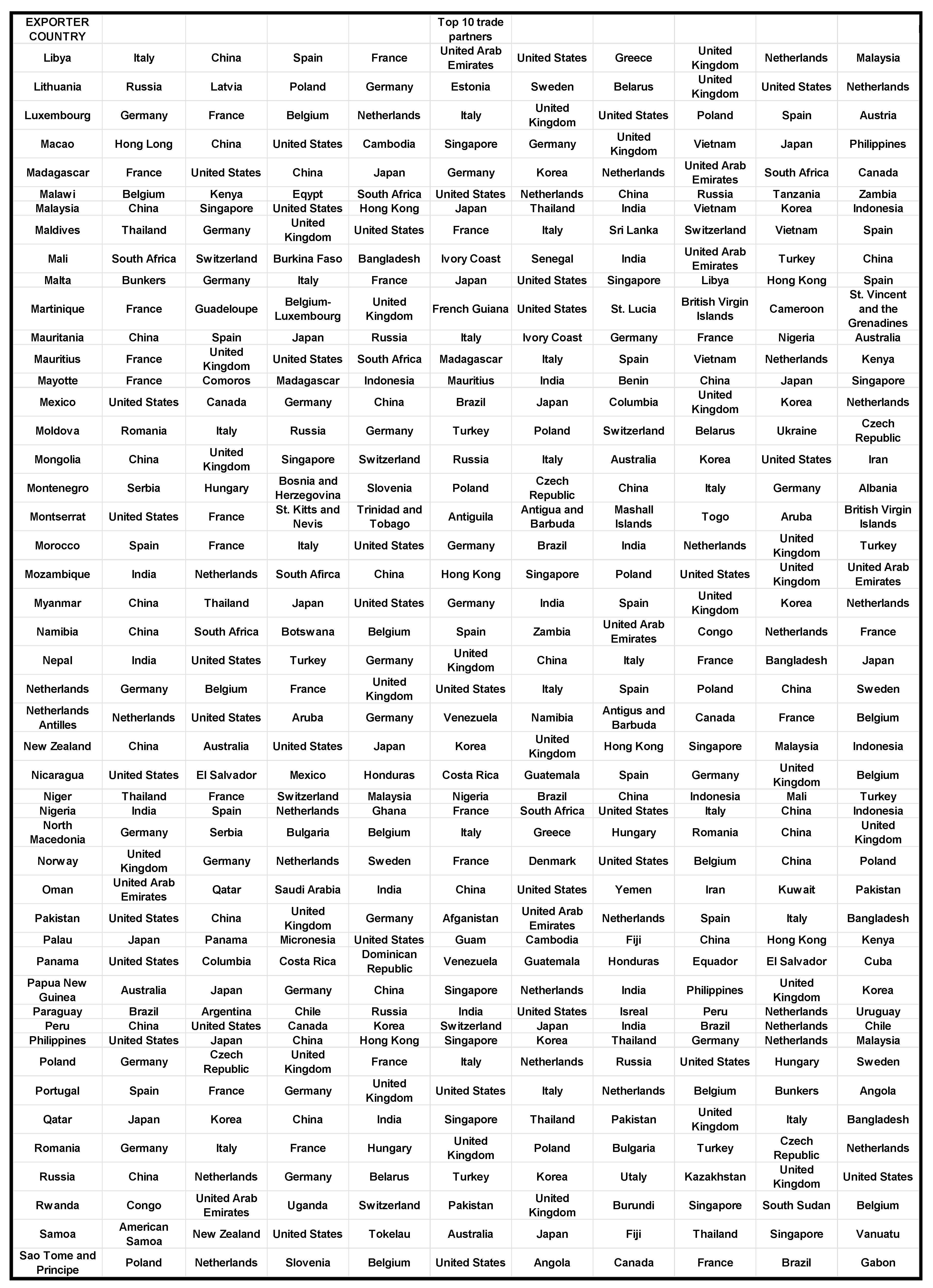
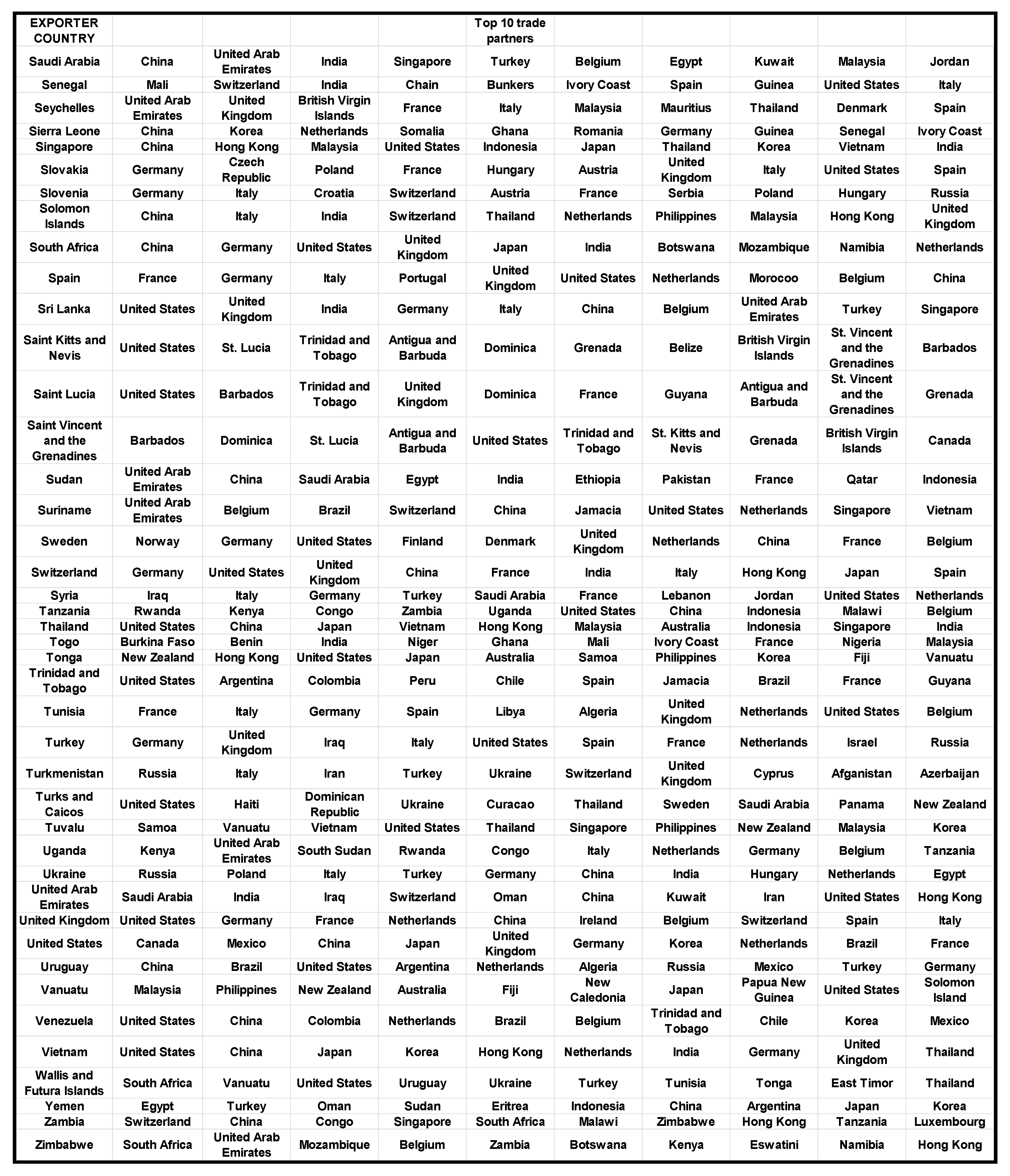
Appendix D
The t-stat of the difference is calculated using the formula
where the null hypothesis is , x and y are the values of the bars, i.e., the percentage of countries with a positive coefficient, , , , and are the sample means and standard deviations constructed by setting the value of the country observation where there is a significant positive coefficient to 1 and 0 if it is not positively significant, and are the two sample sizes.
Appendix E
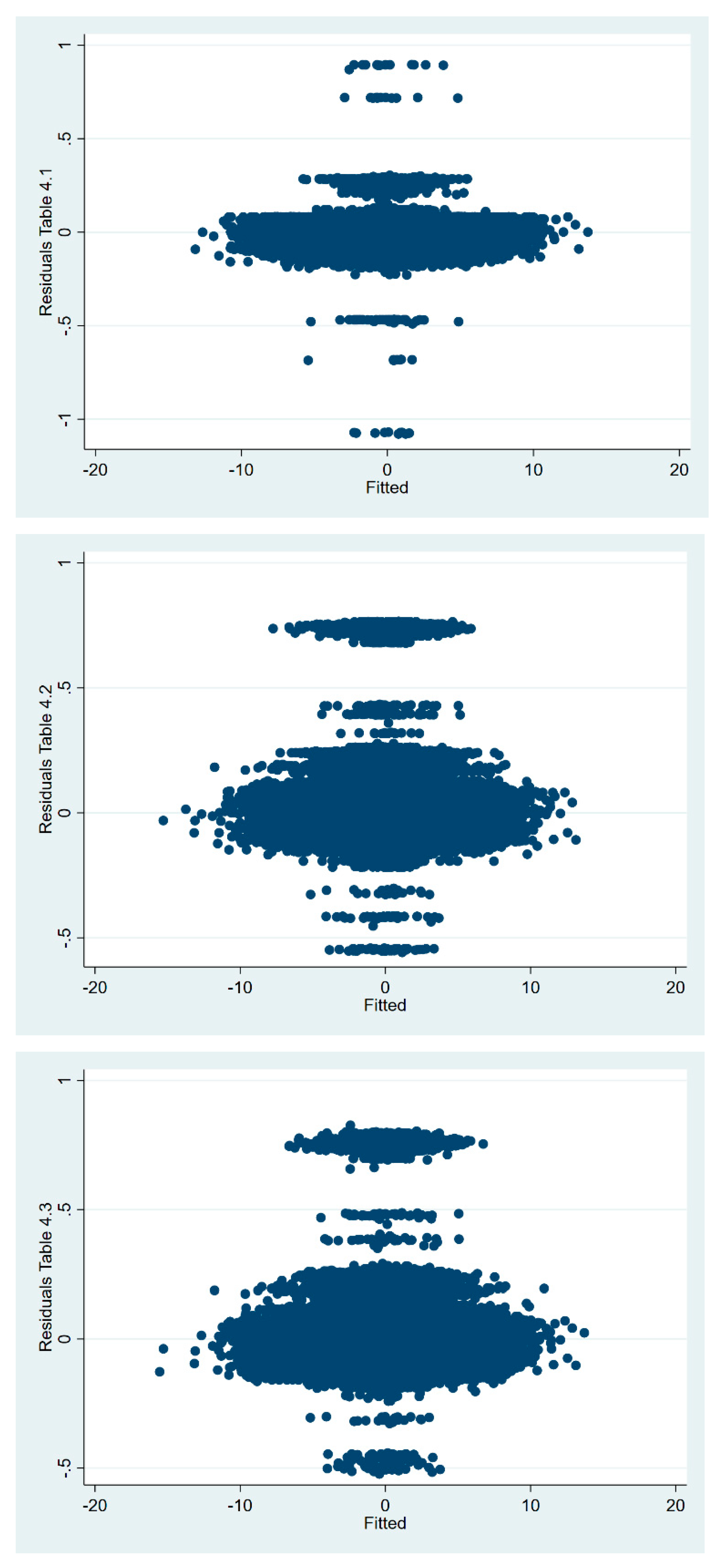
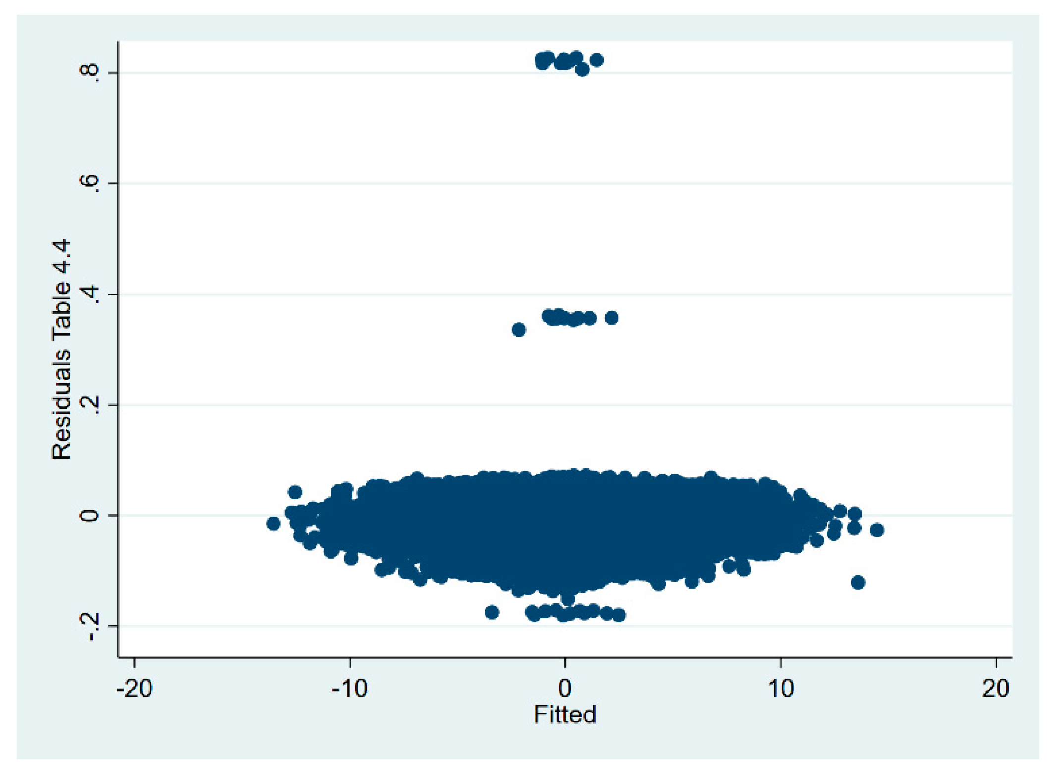
Appendix F
| Table 4’s first Stage Regression: | Dependent variable: Log skill level | ||
| Log skill level first lag | 0.22 (82.3) *** | Services exporter dummy | −0.01 (−74.02) *** |
| Log skill level second lag | −0.24 (−89.65) *** | Fuel exporter dummy | 0.02 (9.01) *** |
| Low income dummy | −0.003 (−13.89) *** | Constant | 0.06 (60.09) *** |
| High income dummy | 0.007 (49.27) *** | R-squared | 0.22 |
| Manufacturing exporter dummy | −0.001 (−19.72) *** | Observations | 527,441 |
| Table 5’s first Stage Regression: | Dependent variable: Log Capital Per worker | ||
| Log capital per worker first lag | 0.68 (470.88) | Services exporter dummy | 0.002 (30.59) |
| Log capital per worker second lag | −0.68 (−461.78) | Fuel exporter dummy | −0.01 (−16.08) |
| Low income dummy | −0.002 (−12.52) | Constant | 0.02 (16.27) |
| High income dummy | −0.002 (−16.67) | R-squared | 0.63 |
| Manufacturing exporter dummy | 0.01 (145.6) | ||
| Table 6’s first Stage Regression: | Dependent variable: Log PGDP | ||
| Log PGDP first lag | 0.34 (217.72) *** | Services exporter dummy | 0.0001 (0.73) |
| Log PGDP second lag | −0.35 (−223.44) *** | Fuel exporter dummy | −0.02 (−24.83) *** |
| Low income dummy | −0.02 (−68.14) *** | Constant | 0.07 (21.47) *** |
| High income dummy | 0.01 (54.13) *** | R-squared | 0.34 |
| Manufacturing exporter dummy | 0.01 (189.82) *** | ||
| Table 7’s first Stage Regression: | Dependent variable: Log skill level | ||
| Log skill level first lag | 0.06 (42.23) | Services exporter dummy | 0.03 (55.53) |
| Log skill level second lag | −0.101 (−77.45) | Fuel exporter dummy | −0.02 (−36.89) |
| Low income dummy | 0.001 (2.78) | Constant | 0.19 (152.57) |
| High income dummy | 0.01 (44.73) | R-squared | 0.17 |
| Manufacturing exporter dummy | −0.01 (−79.23) | ||
| Table 8’s first Stage Regression: | Dependent variable: Log PGDP | ||
| Log PGDP first lag | −0.32 (−156.99) *** | Services exporter dummy | 0.01 (95.99) *** |
| Log PGDP second lag | 0.30 (148.77) *** | Fuel exporter dummy | −0.03 (−49.67) *** |
| Low income dummy | 0.01 (25.62) *** | Constant | 0.17 (173.60) *** |
| High income dummy | 0.02 (96.90) *** | R-squared | 0.57 |
| Manufacturing exporter dummy | 0.02 (179.13) *** |
* significant at 10%; ** significant at 5%; *** significant at 1%.
Notes
| 1 | I seek to address within-product changes in unit values and not changes in the product mix. Therefore, the focus is the changing unit value of the same product. Schott (2004) found evidence of within-product specialization among countries in cross-sectional analysis. According to Schott (2004), high- and low-income countries export higher and lower unit value versions, respectively, of the same products. My analysis seeks to address this issue over time to investigate if individual countries move up the value ladder in their existing exports. Thus WPI is used as the deflator for this exercise. |
| 2 | The low R-squared was investigated by residual plots for each of the regressions in Table 4, Table 5, Table 6, Table 7 and Table 8. These are presented in Appendix E. The residuals are randomly distributed around 0 when plotted against the fitted value of the equation. The low R-squared appears to come from the noisiness of the data, and the trends we find are still significant and practically meaningful. |
| 3 | Each table’s cell gives the proportion of countries with a significant regression coefficient on the factor accumulation variable. For example, in the first cell, six out of 23—approximately 25%—of high-income countries, in 1989–2001, have a significant positive coefficient on skill accumulation. |
| 4 | Further details are presented in Appendix D. |
References
- Aiginger, Karl. 1998. Unit Values to Signal the Quality Position of CEECS. In The Competitiveness of Transition Economies. Paris: OECD. [Google Scholar]
- Alper, A., S. Webb, and J. Oatis. 2019. U.S.-China Trade War—The Levers Each Country Can Pull. World News. Ann Arbor: Thomson Reuters News Agency. [Google Scholar]
- Balassa, Bela. 1979. The changing pattern of comparative advantage in manufactured goods. The Review of Economics and Statistics 61: 259–66. [Google Scholar] [CrossRef]
- Baldwin, Richard. 2016. The World Trade Organization and the future of multilateralism. Journal of Economic Perspectives 30: 95–116. [Google Scholar] [CrossRef] [Green Version]
- Baldwin, John R., and Wulong Gu. 2003. Export-market participation and productivity performance in Canadian manufacturing. Canadian Journal of Economics/Revue Canadienne D’économique 36: 634–57. [Google Scholar] [CrossRef]
- Barro, Robert J. 1991. Economic Growth in a Cross Section of Countries. The Quarterly Journal of Economics 106: 407–43. [Google Scholar] [CrossRef] [Green Version]
- Barro, Robert J., and Jong-Wha Lee. 2001. International data on educational attainment: Updates and implications. Oxford Economic Papers 53: 541–63. [Google Scholar] [CrossRef]
- Bernard, Andrew B., Bradford J. Jensen, and Peter K. Schott. 2006. Survival of the best fit: Exposure to low-wage countries and the (uneven) growth of US manufacturing plants. Journal of international Economics 68: 219–37. [Google Scholar] [CrossRef] [Green Version]
- Brambilla, Irene, Amit K. Khandelwal, Peter K. Schott, and Joseph Francois. 2010. China’s Experience under the Multi-Fiber Arrangement (MFA) and the Agreement on Textiles and Clothing (ATC). Chicago: University of Chicago Press, pp. 345–96. [Google Scholar]
- Chor, D. 2010. Unpacking sources of comparative advantage: A quantitative approach. Journal of International Economics 82: 152–67. [Google Scholar] [CrossRef] [Green Version]
- Costinot, A., D. Donaldson, and I. Komunjer. 2011. What goods do countries trade? A quantitative exploration of Ricardo’s ideas. The Review of Economic Studies 79: 581–608. [Google Scholar] [CrossRef]
- Fabrizio, S., D. Igan, and A. Mody. 2007. The Dynamics of Product Quality and International Competitiveness. IMF Working Paper WP/07/97. Washington, DC: International Monetary Fund. [Google Scholar]
- Feenstra, Robert C., Robert E. Lipsey, and Harry P. Bowen. 1997. World Trade Flows, 1970–1992, with Production and Tariff Data. NBER Working Paper Series No. 5910. Cambridge: National Bureau of Economic Research. [Google Scholar]
- Feenstra, Robert C., Robert E. Lipsey, Haiyan Deng, Alyson C. Ma, and Hengyong Mo. 2005. World Trade Flows: 1962–2000. Cambridge: Natioinal Bureau of Economic Research. [Google Scholar]
- Flam, Harry, and Elhanan Helpman. 1987. Vertical Product Differentiation and North-South Trade. The American Economic Review 77: 810–22. [Google Scholar]
- Fouquin, M., and J. Hugot. 2016. Two Centuries of Bilateral Trade and Gravity data: 1827–2014. No. 015129. Bogotá: Universidad Javeriana-Bogotá. [Google Scholar]
- Grossman, Gene M., and Elhanan Helpman. 1989. Product Development and International Trade. The Journal of Political Economy 97: 1261–83. [Google Scholar] [CrossRef] [Green Version]
- Grossman, Gene M., and Elhanan Helpman. 1991a. Quality Ladders in the Theory of Growth. The Review of Economic Studies 58: 43–61. [Google Scholar] [CrossRef] [Green Version]
- Grossman, Gene M., and Elhanan Helpman. 1991b. Trade, knowledge spillovers, and growth. European Economic Review 35: 517–26. [Google Scholar] [CrossRef] [Green Version]
- Hallak, Juan Carlos. 2006. Product quality and the direction of trade. Journal of International Economics 68: 238–65. [Google Scholar] [CrossRef]
- Hallak, Juan Carlos. 2010. A product-quality view of the Linder hypothesis. The Review of Economics and Statistics 92: 453–66. [Google Scholar] [CrossRef] [Green Version]
- Hallak, Juan Carlos, and Peter K. Schott. 2011. Estimating cross-country differences in product quality. The Quarterly Journal of Economics 126: 417–74. [Google Scholar] [CrossRef] [Green Version]
- Helpman, Elhanan, and Paul R. Krugman. 1985. Market Structure and Foreign Trade. Cambridge: MIT Press. [Google Scholar]
- Hummels, David, and Peter J. Klenow. 2005. The Variety and Quality of a Nation’s Trade. American Economic Review 95: 704–23. [Google Scholar] [CrossRef] [Green Version]
- Jin, H., and K. Takenaka. 2019. Japan-South Korea Feud Deepens with Disputed Accounts of Trade Meeting. World News. Ann Arbor: Thomson Reuters News Agency. [Google Scholar]
- Khandelwal, Amit. 2010. The long and short (of) quality ladders. The Review of Economic Studies 77: 1450–76. [Google Scholar] [CrossRef]
- Linder, Staffan Burenstam. 1961. An Essay on Trade and Transformation. New York: Wiley & Sons. [Google Scholar]
- Mason, J. 2019. Risks Aside, Trump’s Team Sees China Trade Stance as Strength in 2020. Business News. Ann Arbor: Thomson Reuters News Agency. [Google Scholar]
- Mukerji, Purba. 2013. State of Technology and Growth of the Extensive Margin. Scottish Journal of Political Economy 60: 390–411. [Google Scholar] [CrossRef]
- Mukerji, Purba, and John Struthers. 2021. Armington elasticity and development. Journal of Industry, Competition and Trade 21: 59–79. [Google Scholar] [CrossRef]
- Payosova, Tetyana, Gary Clyde Hufbauer, and Jeffrey J. Schott. 2018. The Dispute Settlement Crisis in the World Trade Organization: Causes and Cures. Policy Brief No. PB18-5. Washington, DC: Peterson Institute for International Economics. [Google Scholar]
- Radjou, Navi, Jaideep Prabhu, and Simone Ahuja. 2012. Jugaad Innovation: Think Frugal, Be Flexible, Generate Breakthrough Growth. San Francisco: Wiley. [Google Scholar]
- Regan, M. P., and E. Barrett. 2019. Markets That Priced in a Trade Skirmish Now Brace for a Bruising Fight. Bloomberg Businessweek, May 16. [Google Scholar]
- Romalis, John. 2004. Factor Proportions and the Structure of Commodity Trade. The American Economic Review 94: 67–97. [Google Scholar] [CrossRef] [Green Version]
- Schott, Peter K. 2002. Moving Up and Moving Out: US Product-Level Exports and Competition from Low Wage Countries. New Haven: Yale School of Management. [Google Scholar]
- Schott, Peter. 2004. Across-Product Versus Within-Product Specialization in International Trade. Quarterly Journal of Economics 119: 647–78. [Google Scholar] [CrossRef]
- Summers, Robert. 1995. Penn World Table Mark 5.6 Revision of Summers and Heston (1991) on-Line Data. Computing in the Humanities and Social Sciences (CHASS). Toronto: University of Toronto. [Google Scholar]
- Verhoogen, Eric. A. 2008. Trade, Quality Upgrading and Wage Inequality in the Mexican Manufacturing Sector. The Quarterly Journal of Economics 123: 489–530. [Google Scholar] [CrossRef] [Green Version]
- Vernon, Raymond. 1966. International investment and international trade in the product cycle. The Quarterly Journal of Economics 80: 190–207. [Google Scholar] [CrossRef]
- Wooldridge, Jeffrey M. 2010. Econometric Analysis of Cross Section and Panel Data. Cambridge: MIT Press. [Google Scholar]
Publisher’s Note: MDPI stays neutral with regard to jurisdictional claims in published maps and institutional affiliations. |
© 2021 by the author. Licensee MDPI, Basel, Switzerland. This article is an open access article distributed under the terms and conditions of the Creative Commons Attribution (CC BY) license (https://creativecommons.org/licenses/by/4.0/).