A Discount Technique-Based Inventory Management on Electronics Products Supply Chain

1. Introduction and Literature Review

Inventory management is a technique that will provide benefits within the limited resources. So, properly handling of products always make sense in supply chain management. Although there are many players in the supply chain, this study is based on the end deciding player, the retailer. Storage problems have been discussed over the decades in inventory management. To solve this problem, some researchers suggested hiring warehouses and run a business with two warehouses with one is own and another one is rented (Mashud et al. 2021; Rana et al. 2021; Manna et al. 2021). Sometimes renting a warehouse becomes challenging such as in some elite cities and elite places. However, the benefits of two warehouses also depend on the fare and transportation facility, transportation cost, and suitable places for delivering products. Sometimes all these issues demand more expenses than to sell the products at a marginal discount rate.

The discount facility is a marketing strategy used by the business owner in every layer of the supply chain that has been practiced over the years. Many studies have already been conducted on the benefits and disadvantages of discount policy (Ahn et al. 2009; Bhaula et al. 2019; Zhou 2012). Despite some facilities, it has some drawbacks if the business owner does not offer it with proper management. Discount on selling price is the most common discount approach practiced by the retailer (Zhou 2012). Other than these discounts, a quantity discount, discount on installments, discount on defective items have been discussed parallel by the practitioners. Discounting is a process that will help the retailer to sell the desired products in a quicker time. In other words, a discount policy helps the retailer to accumulate revenue from the market. Moreover, it helps the retailer to overcome any challenging situation for him. In this study, when the quantity of goods is massive in amount, and the retailer has no capacity to store in the warehouse and significantly needs liquid money, the retailer offers a marginal discount by adjusting the market selling price.

Selling price is one of the critical factors that need equal attention to other logistics activities on inventory management. A retailer always has to offer a realistic selling price to its customers by adjusting the purchase cost of the respective products as the selling price plays an integral part in the chain. It has been often observed that the business owner chooses to discount the selling price (Md Mashud et al. 2020). However, this discount sometimes depends on the stock of the products (Ahn et al. 2009).

The stock of products in the warehouse has some direct and indirect consequences in the market, especially when a retailer is fixing the selling price of the products. A massive study has been studied on stock-dependent demand (Chandra 2017; Shah and Naik 2018; Shaikh et al. 2019). This stock-dependent demand sometimes depends on time because as time progress in the chain, the stock is depleted to satisfy the customer’s demand, so an indirect relationship between time and stock has been noticed. This paper will link all these crucial issues, as time, price, and stock-dependent demand have been considered. Some other contributions of the paper are:

• It critically evaluates when one needs to impose a discount and when to not, especially when a bulk purchase has been made by a retailer with a huge investment in a limited storage shop in a highly expensive location.
• A synergy between stock, price, and time-dependent demand and implications of discount policy has been meticulously explained.
• A sensitivity analysis with some theoretical findings has been suggesting to achieve the maximum profit in the chain for the managers of the industry and shown a threshold point of discount offered time.

In the rest of the study, we have arranged the manuscript with the literature review in Section 1.1 followed by Section 2 wherein a problem description with notations and assumptions has been provided. In contrast, in Section 3, the mathematical form of the study has been studied. In Section 4, the theoretical derivations, whereas in Section 4.1, some numerical examples and graphs are presented. Finally, sensitivity and managerial insights have been provided in Section 4.2, with a conclusion and future scope in Section 5.

1.1. Literature Review

This study mainly focused on four components of an electronic products supply chain. The first one is stock availability, price sensitivity, the impact of time, and the influence of discounts.

1.1.1. Influence of Stock Dependent Demand on Traditional Inventory Model

The first execution of the economic order quantity model by (Harris 1990) opens the border for the inventory researcher. It capitalizes later by inventory researchers employing some realistic assumptions, for example, stock of products, discount policy, effects of time, and many other widely used attributes in the field of supply chain management. Sometimes a large inventory of products in any store can entice customers and produce higher demand than usual (Macías-López et al. 2021; Chang et al. 2010). In this direction, (Gupta and Vrat 1986) was the pioneer to explore the first inventory model with a stock-dependent demand rate. (Datta et al. 1998) updated the existing system of inventory model by introducing demand promotion under its stock-dependency behavior. They conducted a study on how demand changed with the upgrades, and based on this survey, they had to decide how many upgrades would be successful at maximizing profits. Later, (Cárdenas-Barrón et al. 2020) developed two inventory models according to the retailer’s perspective considering demand to be nonlinearly stock dependent, including trade credit period offer for the supplier. (Halim et al. 2021) adopted nonlinear price and stock-related market demand for deteriorating items in their production model. (Pando et al. 2021) analyzed a deterministic inventory model with stock-dependent demand, focusing on maximizing returns on investments rather than maximizing profits.

1.1.2. Influence of Price Sensitive Demand on Tradition Inventory Model

The price of the products can drive the uneven nature of the demand of the customers. Higher price always has some disadvantages to reduce the number of demands while a lower price can significantly entice new demands. For retailing businesses, it is imperative to plug inappropriate price tags for appropriate products to run business smoothly; otherwise, the retailer may face some loss in business. (Liu et al. 2021) contemplated price-sensitive demand for perishable products in a two-echelon supply chain model and explained its importance by showing the effects of price sensitivity on the collection, production, and sales. Considering the retailer’s profit growth, (Paul et al. 2021) developed an EOQ model for deteriorating items under selling price-sensitive demand with default risk and then discussed their impact during the optimal cycle time and credit period. (De-la-Cruz-Márquez et al. 2021) focused on sustainability issues by introducing the concept of carbon emissions, including price-sensitive demand rates for imperfect quality items.

1.1.3. Influence of Sensitiveness of Time on Traditional Inventory Mode

Over the years in inventory research, time-varying demand has had a significant role in decision making and got the attention of the respective field scholars. The first model introduced the concept of time-varying demand to inventory management and projected an economic order quantity model without considering shortages but deteriorating items (Donaldson 1977). However, the solution procedure of that model was too perplexing and later led to meta-heuristics techniques. Modifying Donaldson’s model, an inventory model for shortage items for deteriorating items with the same demand has been anticipated (Chang and Dye 1999). Later, this shortages concept was changed to an exponential type backlogged with time-varying demand for deteriorating items (Papachristos and Skouri 2000). (Adak and Mahapatra 2020) presented a cost-effective multi-item EOQ model where demand rate was considered dependent on advertising, time, and reliability. As consumers are now more health-conscious than ever before, the demand for fresh items has increased sharply. Based on this concept, (Macías-López et al. 2021) developed a model for perishable items that emphasizes customer demand with product quality over time. The demand here is considered with selling price and available stock dependent. Next, (San-José et al. 2021) included time-related demand functions in the power pattern in his proposed model where shortages were partially backlogged.

1.1.4. Impacts of Discount Policy on Electronic Products

Discount is a vital marketing policy being used in smoothing the business or for quick recovery. The discount on price is widely used in extant literature. (Ahn et al. 2009) provided a discount in inventory models and the effect of time on it. (Hasan et al. 2020) anticipated an inventory model for pre-order discounts in an online payment system. (Latha et al. 2021) developed a model for a two-echelon system for backorder price discounts to entice the customers when shortages occur in the chain while (Limansyah et al. 2020) provided an economic order quantity model for all unit discount policy. Prior studies show numerous types of discount policies in present inventory management and supply chain management. Still, to our best of knowledge, no one considers price discounts for such situations as presented in the model. We have presented the discount policy so that it will reduce the risk of investment and help the manager recover the capital quickly, which is rare in prior studies. The fundamental contribution is that a retailer thus completes a bulk purchase and strives for quick capital recovery. Suppose he has to pay considerable expenses to hold the products because of the store’s location, in that case, he can run his business smoothly and earn his expected profit based on the pricing strategies and discount policy given in this proposed study.

2. Assumption and Notations

For a clear demonstration of the mathematical model in this paper, some assumptions and notations were considered which are listed below in Section 2.1 and Section 2.2.

2.1. Assumptions

The mathematical model proposed in this paper is based on the following assumptions.

• The replenishment rate is infinite and Lead-time is negligible.
• This model is for a single type of item.
• The planning horizon is considered infinite.
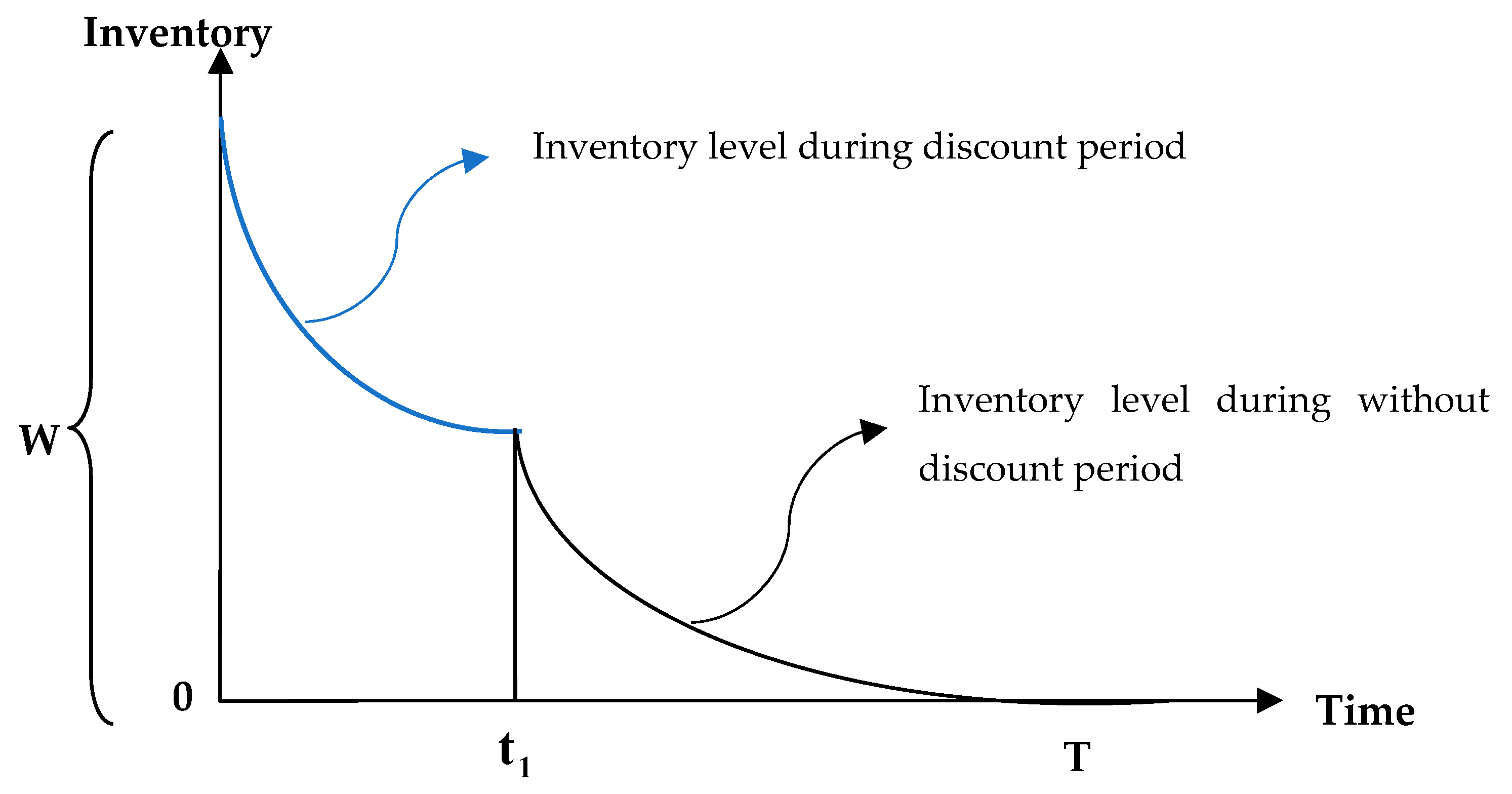
• In this paper, the demand function comprises price, time, and stock-dependence in the form of

  $$D=\{\begin{array}{l}\left(a-bp\left(1-\delta \right)\right)+\alpha t+\beta t^2+s{I}_1(t),\mathrm{when}\hspace{0.17em}0\le t\le t_1\left(\mathrm{discount}\mathrm{is}\mathrm{given}\mathrm{on}\mathrm{price}\right)\\ (a-bp)+\alpha t+\beta t^2+s{I}_2(t),\hspace{0.17em}\mathrm{when}\hspace{0.17em}{t}_1<t\le T\hspace{0.17em}\left(\mathrm{without}\mathrm{discount}\right)\end{array}$$

  where,
  $a$ is the initial rate of demand
  $b$ is the rate decrease demand on prices
  $p$ is the product price
  $\delta$ is the discount rate on price of product
  $\alpha$ is the rate with which the demand rate increases on time
  $\beta$ is the rate of changes of rate on time in the demand rate itself
  $s$ is the rate depending on stock, $0<s\le 1$
• There are no shortages considered in this model.

2.2. Notations

The notations that we need to construct the model is given in

Table 1. Notations description.

Notations	Units	Description
$C$	$/Cycle	Ordering cost per cycle
$C_p$	$/Unit	Purchasing cost per unit
$C_h$	$/Unit	Holding cost per unit per unit time
$w$	Units/Cycle	Ordering quantity per cycle
$T_{fc}$	$/Cycle	Fixed transportation cost
$T_{vc}$	$/unit	Variable transportation cost
$t_1$	Months	Discount time from the beginning of cycle
$D$	Units	Demand function
$I_i\left(t\right)$	Units	inventory level at any time t where $0\le t\le t_1$ when i = 1, $t_1\le t\le T$ when i = 2
$\delta$	Constant	Discount rate on price of product
$\omega \left(p,T\right)$	$/Month	Total profit per unit time
Decision variables
$p$	$/Unit	Selling price per unit of product
$T$	Months	replenishment time.

.

3. Mathematical Formulation for Proposed Electronics Product Inventory Model

Based on the above-mentioned assumptions, we built an inventory model. Initially, an enterprise purchased $w$ units of goods. Considering the above assumptions, the inventory level tracks the pattern depicted in the following Figure 1.

To meet up the customer’s demands, this stock depleted. The enterprise gives a discount on price at 0 to $t_1$ times after the time the discount is closed. As a result, at time $t=T$ the stock will become zero. Thus, the inventory system is described by the ensuing a differential equation in view of demand $D=a-b\hspace{0.17em}p\hspace{0.17em}\left(1-\delta \right)+\alpha \hspace{0.17em}t+\beta \hspace{0.17em}{t}^2+s\hspace{0.17em}{I}_1(t)$:

$$\frac{d{I}_1(t)}{dt}=-D 0\le t\le t_1.$$

(1)

with the condition $I_1(t)=w\hspace{0.17em}at\hspace{0.17em}t=0$.

After closing the discount, the demand $D=a-b\hspace{0.17em}p\hspace{0.17em}+\alpha \hspace{0.17em}t+\beta \hspace{0.17em}{t}^2+s\hspace{0.17em}{I}_2(t)$, the differential equation is

$$\frac{d{I}_2(t)}{dt}=-D t_1\le t\le T$$

(2)

with $I_2(t)=0\hspace{0.17em}at\hspace{0.17em}t=T$, $I_1(t)\hspace{0.17em},I_2(t)$ is continuous at $t=t_1$.

3.1. Solution of Differential Equations from (1) and (2)

With the help of boundary conditions $I_1(t)=w$ at $t=0$ after solving Equation (1) we get:

$$I_1\left(t\right)=\frac{bp-a-b\delta p-\alpha t-\beta t^2}{s}+\frac{\alpha +2\beta t}{s^2}-\frac{2\beta }{s^3}+\left(w+\frac{b\delta p-bp+a}{s}-\frac{\alpha }{s^2}+\frac{2\beta }{s^3}\right)e^{-st}$$

(3)

where $0\le t\le t_1$.

With the help of boundary conditions $I_2(t)=0$ at $t=T$ after solving Equation (2) we get:

$$I_2\left(t\right)=\frac{bp-a-\alpha t-\beta t^2}{s}+\frac{\alpha +2\beta t}{s^2}-\frac{2\beta }{s^3}-\left(\frac{bp-a-\alpha T-\beta T^2}{s}+\frac{\alpha +2\beta T}{s^2}-\frac{2\beta }{s^3}\right)e^{s\left(T-t\right)}$$

(4)

where $t_1\le t\le T$.

Applying continuity at $t=t_1$ we can write $I_1(t_1)=I_2(t_1)$ which implies that,

$$w=\left\{\begin{array}{l}\frac{b\delta p}{s}{e}^{s{t}_1}-\left(\frac{bp-a-\alpha T-\beta T^2}{s}+\frac{\alpha +2\beta T}{s^2}-\frac{2\beta }{s^3}\right)e^{sT}\\ -\left(\frac{b\delta p-bp+a}{s}-\frac{\alpha }{s^2}+\frac{2\beta }{s^3}\right)\end{array}\right\}$$

(5)

The total cost per unit time for the inventory system contains of the subsequent constituents.

3.2. The Total Cost per Unit Time per Cycle

(a)

Ordering cost per cycle = $C$

(b)

Holding cost (HC) = $C_h\left[{\displaystyle \underset{0}{\overset{t_1}{\int }}{I}_1(t)\hspace{0.17em}dt}+{\displaystyle \underset{t_1}{\overset{T}{\int }}{I}_2(t)\hspace{0.17em}dt}\right]$

i.e.,

$$C_h\left[\begin{array}{l}\left(\frac{bp-a}{s}+\frac{\alpha }{s^2}-\frac{2\beta }{s^3}\right)T+\left(\frac{2\beta }{s^2}-\frac{\alpha }{s}\right)\frac{T^2}{2}+\left(\frac{w}{s}+\frac{b\delta p-bp+a}{s^2}-\frac{\alpha }{s^3}+\frac{2\beta }{s^4}\right)\left(1-e^{s{t}_1}\right)+\\ \left(\frac{bp-a-\alpha T-\beta T^2}{s^2}+\frac{\alpha +2\beta T}{s^3}-\frac{2\beta }{s^4}\right)\left(1-e^{s\left(T-t_1\right)}\right)-\frac{b\delta p{t}_1}{s}-\frac{\beta T^3}{3s}\end{array}\right]$$

(6)

(c)

Purchase cost (PC) = $C_p{}^{*}w$

$$C_p\left[\frac{b\delta p}{s}{e}^{s{t}_1}-\left(\frac{bp-a-\alpha T-\beta T^2}{s}+\frac{\alpha +2\beta T}{s^2}-\frac{2\beta }{s^3}\right)e^{sT}-\left(\frac{b\delta p-bp+a}{s}-\frac{\alpha }{s^2}+\frac{2\beta }{s^3}\right)\right]$$

(7)

(d)

Transportation cost (TC) = $T_{fc}+T_{vc}{}^{*}w$

$$T_{fc}+T_{vc}\left[\begin{array}{l}\frac{b\delta p}{s}{e}^{s{t}_1}-\left(\frac{bp-a-\alpha T-\beta T^2}{s}+\frac{\alpha +2\beta T}{s^2}-\frac{2\beta }{s^3}\right)e^{sT}\\ -\left(\frac{b\delta p-bp+a}{s}-\frac{\alpha }{s^2}+\frac{2\beta }{s^3}\right)\end{array}\right]$$

(8)

(e)

Sales revenue (SR) = $p^{*}\left[{\displaystyle {\int }_0^{t_1}D\hspace{0.17em}dt+{\displaystyle \underset{t_1}{\overset{T}{\int }}D\hspace{0.17em}dt}}\right]$

$$=p^{*}\left[{\displaystyle {\int }_0^{t_1}\left(a-b\hspace{0.17em}p\hspace{0.17em}\left(1-\delta \right)+\alpha \hspace{0.17em}t+\beta \hspace{0.17em}{t}^2+s\hspace{0.17em}{I}_1(t)\right)\hspace{0.17em}dt+{\displaystyle \underset{t_1}{\overset{T}{\int }}\left(a-b\hspace{0.17em}p\hspace{0.17em}+\alpha \hspace{0.17em}t+\beta \hspace{0.17em}{t}^2+s\hspace{0.17em}{I}_2(t)\right)\hspace{0.17em}dt}}\right]$$

$$\begin{array}{l}=\left(a-bp\right)pT+\frac{\alpha p{T}^2}{2}+\frac{\beta p{T}^3}{3}+b{p}^2\delta t_1+\\ sp\left[\begin{array}{l}\left(\frac{bp-a}{s}+\frac{\alpha }{s^2}-\frac{2\beta }{s^3}\right)T+\left(\frac{2\beta }{s^2}-\frac{\alpha }{s}\right)\frac{T^2}{2}+\left(\frac{w}{s}+\frac{b\delta p-bp+a}{s^2}-\frac{\alpha }{s^3}+\frac{2\beta }{s^4}\right)\left(1-e^{s{t}_1}\right)+\\ \left(\frac{bp-a-\alpha T-\beta T^2}{s^2}+\frac{\alpha +2\beta T}{s^3}-\frac{2\beta }{s^4}\right)\left(1-e^{s\left(T-t_1\right)}\right)-\frac{b\delta p{t}_1}{s}-\frac{\beta T^3}{3s}\end{array}\right]\end{array}$$

(9)

Now, the total profit per unit time one can write as

$$\omega \left(p,T\right)=\frac{1}{T}\left(SR-C-HC-PC-TC\right)$$

$$\omega \left(p,T\right)=\frac{1}{T}\left(\begin{array}{l}\left(sp-C_h\right)\left[\begin{array}{l}\left(\frac{bp-a}{s}+\frac{\alpha }{s^2}-\frac{2\beta }{s^3}\right)T+\left(\frac{2\beta }{s^2}-\frac{\alpha }{s}\right)\frac{T^2}{2}-\frac{b\delta p{t}_1}{s}-\frac{\beta T^3}{3s}\\ +\left(\frac{w}{s}+\frac{b\delta p-bp+a}{s^2}-\frac{\alpha }{s^3}+\frac{2\beta }{s^4}\right)\left(1-e^{s{t}_1}\right)\\ +\left(\frac{bp-a-\alpha T-\beta T^2}{s^2}+\frac{\alpha +2\beta T}{s^3}-\frac{2\beta }{s^4}\right)\left(1-e^{s\left(T-t_1\right)}\right)\end{array}\right]\\ +\left(a-bp\right)pT+\frac{\alpha p{T}^2}{2}+\frac{\beta p{T}^3}{3}+b{p}^2\delta t_1-C-T_{fc}-\\ \left(T_{vc}+C_p\right)\left[\begin{array}{l}\frac{b\delta p}{s}{e}^{s{t}_1}-\left(\frac{bp-a-\alpha T-\beta T^2}{s}+\frac{\alpha +2\beta T}{s^2}-\frac{2\beta }{s^3}\right)e^{sT}\\ -\left(\frac{b\delta p-bp+a}{s}-\frac{\alpha }{s^2}+\frac{2\beta }{s^3}\right)\end{array}\right]\end{array}\right)$$

(10)

with

$$\begin{array}{l}D=a-b\hspace{0.17em}p\hspace{0.17em}\left(1-\delta \right)+\alpha \hspace{0.17em}t+\beta \hspace{0.17em}{t}^2+s\hspace{0.17em}{I}_1(t)>0;\\ p<\frac{a}{b};\\ T>0;\\ p>C_p;\end{array}\}$$

(11)

4. Theoretical Derivations

The concavity of the profit function is validating through some propositions with the help of the (Cambini and Martein 2009) theorem on fractional programming.

Lemma 1.

Let$\omega \left(x\right)=\frac{\phi \left(x\right)}{\psi \left(x\right)}$. If$\phi$ is non-negative and concave, and $\psi$ is positive and convex, then $\omega$ is semi-strictly quasiconcave.

Proof. 

See (Cambini and Martein 2009) for details. □

Put $w$ value from Equation (5) into Equation (10), one can get the objective function as follows

$$\omega \left(p,T\right)=\frac{1}{T}\left[\begin{array}{l}\left(sp-C_h\right)\left[\begin{array}{l}\left(\frac{bp-a}{s}+\frac{\alpha }{s^2}-\frac{2\beta }{s^3}\right)T+\left(\frac{2\beta }{s^2}-\frac{\alpha }{s}\right)\frac{T^2}{2}-\frac{b\delta p{t}_1}{s}-\frac{\beta T^3}{3s}\\ +\left(\frac{b\delta p-bp+a}{s^2}-\frac{\alpha }{s^3}+\frac{2\beta }{s^4}\right)\left(1-e^{s{t}_1}\right)\\ +\left(\frac{bp-a-\alpha T-\beta T^2}{s^2}+\frac{\alpha +2\beta T}{s^3}-\frac{2\beta }{s^4}\right)\left(1-e^{s\left(T-t_1\right)}\right)\end{array}\right]\\ +\left(a-bp\right)pT+\frac{\alpha p{T}^2}{2}+\frac{\beta p{T}^3}{3}+b{p}^2\delta t_1-C-T_{fc}-\\ \left(\begin{array}{l}{T}_{vc}+C_p+\\ \left(1-e^{s{t}_1}\right)\left(p-\frac{C_h}{s}\right)\end{array}\right)\left[\begin{array}{l}\frac{b\delta p}{s}{e}^{s{t}_1}-\left(\frac{b\delta p-bp+a}{s}-\frac{\alpha }{s^2}+\frac{2\beta }{s^3}\right)\\ -\left(\frac{bp-a-\alpha T-\beta T^2}{s}+\frac{\alpha +2\beta T}{s^2}-\frac{2\beta }{s^3}\right)e^{sT}\end{array}\right]\\ \end{array}\right]$$

(12)

Proposition 1.

The objective function$\omega \left(p,T\right)$presented in Equation (12) demonstrates the concavity in terms of the product selling price$p$when cycle time$T$is considered as constants,${\mathrm{e}}^{s\left(T-t_1\right)}>2e^{s{t}_1}+\delta e^{2s{t}_1}$and the optimal$p^{*}$is characterized by the following equation:

$$p^{*}=\frac{\left[\begin{array}{l}\left(\alpha s-2\beta \right)sT+s^2\beta T^2-s^3\left(T_{vc}+C_p\right)\left(b\delta e^{s{t}_1}-b{e}^{sT}-b\delta +b\right)\\ -\left(\left(a+\alpha T+\beta T^2\right)s^2-\left(\alpha +2\beta T\right)s+2\beta \right)\left(1-e^{s\left(T-t_1\right)}\right)\\ -C_h\left[\left(bT-b\delta t_1\right)s^2+sb\left(\delta \left(1-e^{s{t}_1}\right)+e^{s{t}_1}-e^{s\left(T-t_1\right)}\right)\right]-\\ \left(1-e^{s{t}_1}\right)\left[\begin{array}{l}\left(\left(a+\alpha T+\beta T^2\right)s^2-\left(\alpha +2\beta T-b{C}_h\right)s+2\beta \right)e^{sT}\\ +\left(2\alpha -C_{h}b\left(1-\delta \right)\right)s-b\delta C_{h}s{e}^{s{t}_1}-2a{s}^2-4\beta \end{array}\right]\end{array}\right]}{2b{s}^2\left(e^{s\left(T+t_1\right)}-\delta e^{2s{t}_1}+3\delta e^{s{t}_1}-e^{sT}-2e^{s{t}_1}+e^{s\left(T-t_1\right)}-2\delta +1\right)}$$

(13)

Proof. 

Differentiate Equation (12) regarding $p$, one can get

$$\frac{\partial \omega }{\partial p}=\frac{1}{T{s}^3}\left[\begin{array}{l}\left(\alpha s-2\beta \right)sT+s^2\left(\beta T^2-sbpT+sbp\delta t_1\right)-s^3\left(T_{vc}+C_p\right)\left(\begin{array}{l}b\delta e^{s{t}_1}-b{e}^{sT}\\ -b\delta +b\end{array}\right)\\ +\left(\left(bp-a-\alpha T-\beta T^2\right)s^2+\left(\alpha +2\beta T\right)s-2\beta \right)\left(1-e^{s\left(T-t_1\right)}\right)\\ +\left(sp-C_h\right)\left[\left(bT-b\delta t_1\right)s^2+sb\left(\delta \left(1-e^{s{t}_1}\right)+e^{s{t}_1}-e^{s\left(T-t_1\right)}\right)\right]-\\ \left(1-e^{s{t}_1}\right)\left[\begin{array}{l}\left(2b\delta p{s}^2-b\delta C_{h}s\right)e^{s{t}_1}-\left(\begin{array}{l}\left(2bp-a-\alpha T-\beta T^2\right)s^2\\ +\left(\alpha +2\beta T-b{C}_h\right)s-2\beta \end{array}\right)e^{sT}\\ +\left(3bp\left(1-\delta \right)-2a\right)s^2+\left(2\alpha -C_{h}b\left(1-\delta \right)\right)s-4\beta \end{array}\right]\end{array}\right]$$

(14)

 □

Now $\frac{\partial \omega }{\partial p}=0$ and solve for p, one can find critical point as follows

$$p=\frac{\left[\begin{array}{l}\left(\alpha s-2\beta \right)sT+s^2\beta T^2-s^3\left(T_{vc}+C_p\right)\left(b\delta e^{s{t}_1}-b{e}^{sT}-b\delta +b\right)\\ -\left(\left(a+\alpha T+\beta T^2\right)s^2-\left(\alpha +2\beta T\right)s+2\beta \right)\left(1-e^{s\left(T-t_1\right)}\right)\\ -C_h\left[\left(bT-b\delta t_1\right)s^2+sb\left(\delta \left(1-e^{s{t}_1}\right)+e^{s{t}_1}-e^{s\left(T-t_1\right)}\right)\right]-\\ \left(1-e^{s{t}_1}\right)\left[\begin{array}{l}\left(\left(a+\alpha T+\beta T^2\right)s^2-\left(\alpha +2\beta T-b{C}_h\right)s+2\beta \right)e^{sT}\\ +\left(2\alpha -C_{h}b\left(1-\delta \right)\right)s-b\delta C_{h}s{e}^{s{t}_1}-2a{s}^2-4\beta \end{array}\right]\end{array}\right]}{2b{s}^2\left(e^{s\left(T+t_1\right)}-\delta e^{2s{t}_1}+3\delta e^{s{t}_1}-e^{sT}-2e^{s{t}_1}+e^{s\left(T-t_1\right)}-2\delta +1\right)}$$

(15)

Again, differentiate Equation (14) with respect to $p$

$$\frac{{\partial }^2\omega }{\partial p^2}=-\frac{2b}{sT}\left(e^{sT}\left(e^{s{t}_1}-1\right)+\left(e^{sT-s{t}_1}-2e^{s{t}_1}-\delta e^{2s{t}_1}\right)+\delta \left(3e^{s{t}_1}-2\right)+1\right)$$

(16)

Since ${\mathrm{e}}^{s\left(T-t_1\right)}>2e^{s{t}_1}+\delta e^{2s{t}_1}$, easy to say that, $\frac{{\partial }^2\omega }{\partial p^2}<0$ for any value of $p$. That implies the objective function is a concave function. The critical point $p$ becomes the optimal point $p^{*}$.

Proposition 2.

The objective function$\omega \left(p,T\right)$presented in Equation (12) demonstrates the concavity in terms of cycle time T when the product selling price p is considered as constants.

Proof. 

Similar to Proposition 1. To avoid redundancy, proof has been omitted. □

Proposition 3.

The objective function$\omega \left(p,T\right)$presented in Equation (12) demonstrates the concavity in terms of the product selling price$p$as well as cycle time$T$with the condition

$$\left[\begin{array}{l}2b{\Omega }_1+{\Omega }_4\\ -2b{e}^{sT}\end{array}\right]\left[\left(\begin{array}{l}{\Omega }_3+ps{e}^{sT}\\ -\left(sp-C_h\right){\Omega }_1\end{array}\right)\left(\begin{array}{l}{\Omega }_2+bps\\ +2\beta T+\alpha \end{array}\right)-C_h\left(2\beta T+\alpha \right)\right]>{\left[\begin{array}{l}{\Omega }_1{\Omega }_2+b{C}_h\left({\Omega }_1-1\right)\\ +{\Omega }_{3}b-{\Omega }_2{e}^{sT}\end{array}\right]}^2$$

Proof. 

The profit function per unit time can be written as by using Lemma 1,

$$\omega \left(p,T\right)=\frac{\phi (p,T)}{\psi (p,T)}$$

(17)

where,

$$\phi \left(p,T\right)=\left[\begin{array}{l}\left(sp-C_h\right)\left[\begin{array}{l}\left(\frac{bp-a}{s}+\frac{\alpha }{s^2}-\frac{2\beta }{s^3}\right)T+\left(\frac{2\beta }{s^2}-\frac{\alpha }{s}\right)\frac{T^2}{2}-\frac{b\delta p{t}_1}{s}-\frac{\beta T^3}{3s}\\ +\left(\frac{b\delta p-bp+a}{s^2}-\frac{\alpha }{s^3}+\frac{2\beta }{s^4}\right)\left(1-e^{s{t}_1}\right)\\ +\left(\frac{bp-a-\alpha T-\beta T^2}{s^2}+\frac{\alpha +2\beta T}{s^3}-\frac{2\beta }{s^4}\right)\left(1-e^{s\left(T-t_1\right)}\right)\end{array}\right]\\ +\left(a-bp\right)pT+\frac{\alpha p{T}^2}{2}+\frac{\beta p{T}^3}{3}+b{p}^2\delta t_1-C-T_{fc}-\\ \left(\begin{array}{l}{T}_{vc}+C_p+\\ \left(1-e^{s{t}_1}\right)\left(p-\frac{C_h}{s}\right)\end{array}\right)\left[\begin{array}{l}\frac{b\delta p}{s}{e}^{s{t}_1}-\left(\frac{b\delta p-bp+a}{s}-\frac{\alpha }{s^2}+\frac{2\beta }{s^3}\right)\\ -\left(\frac{bp-a-\alpha T-\beta T^2}{s}+\frac{\alpha +2\beta T}{s^2}-\frac{2\beta }{s^3}\right)e^{sT}\end{array}\right]\end{array}\right]$$

$$\psi \left(p,T\right)=T$$

 □

Since $\psi \left(p,T\right)>0$ is a linear function of $p$, $T$. For showing $\omega \left(p,T\right)$ is a concave function, it is enough to show $\phi \left(p,T\right)$ is a concave function.

The first order partial derivatives of $\phi \left(p,T\right)$ with respect to $p$ and $T$ are as follows:

$$\frac{\partial \omega }{\partial p}=\frac{1}{s^3}\left[\begin{array}{l}\left(\alpha s-2\beta \right)sT+s^2\left(\beta T^2-sbpT+sbp\delta t_1\right)-s^3\left(T_{vc}+C_p\right)\left(\begin{array}{l}b\delta e^{s{t}_1}-b{e}^{sT}\\ -b\delta +b\end{array}\right)\\ +\left(\left(bp-a-\alpha T-\beta T^2\right)s^2+\left(\alpha +2\beta T\right)s-2\beta \right)\left(1-e^{s\left(T-t_1\right)}\right)\\ +\left(sp-C_h\right)\left[\left(bT-b\delta t_1\right)s^2+sb\left(\delta \left(1-e^{s{t}_1}\right)+e^{s{t}_1}-e^{s\left(T-t_1\right)}\right)\right]-\\ \left(1-e^{s{t}_1}\right)\left[\begin{array}{l}\left(2b\delta p{s}^2-b\delta C_{h}s\right)e^{s{t}_1}-\left(\begin{array}{l}\left(2bp-a-\alpha T-\beta T^2\right)s^2\\ +\left(\alpha +2\beta T-b{C}_h\right)s-2\beta \end{array}\right)e^{sT}\\ +\left(3bp\left(1-\delta \right)-2a\right)s^2+\left(2\alpha -C_{h}b\left(1-\delta \right)\right)s-4\beta \end{array}\right]\end{array}\right]$$

(18)

$$\frac{\partial \phi }{\partial T}=\frac{1}{s}\left[\begin{array}{l}\left(sp-C_h\right)e^{s\left(T-t_1\right)}+\left(sp-C_h\right)e^{s\left(T+t_1\right)}\\ -\left(\left(C_p+T_{vc}+p\right)s-C_h\right)e^{sT}+C_h\end{array}\right]\left(\beta T^2+\alpha T-bp+a\right)$$

(19)

The second order partial derivatives of $\phi \left(p,T\right)$ with respect to $p$ and $T$ are as follows:

$$\frac{{\partial }^2\omega }{\partial p^2}=-\frac{2b}{s}\left(e^{sT}\left(e^{s{t}_1}-1\right)+\left(e^{sT-s{t}_1}-2e^{s{t}_1}-\delta e^{2s{t}_1}\right)+\delta \left(3e^{s{t}_1}-2\right)+1\right)$$

(20)

$$\frac{{\partial }^2\phi }{\partial T^2}=-\frac{1}{s}\left[\begin{array}{l}\left(\begin{array}{l}\left(\left(C_p+T_{vc}+p\right)s-C_h\right)e^{sT}\\ -\left(sp-C_h\right)e^{s\left(T-t_1\right)}-\left(sp-C_h\right)e^{s\left(T+t_1\right)}\end{array}\right)\left(\beta T^2+\alpha T-bp+a\right)s\\ +\left(\begin{array}{l}\left(\left(C_p+T_{vc}+p\right)s-C_h\right)e^{sT}-C_h-\\ \left(sp-C_h\right)e^{s\left(T-t_1\right)}-\left(sp-C_h\right)e^{s\left(T+t_1\right)}\end{array}\right)\left(2\beta T+\alpha \right)\end{array}\right]$$

(21)

$$\frac{{\partial }^2\phi }{\partial p\partial T}=\frac{1}{s}\left[\begin{array}{l}\left(\left(T^2\beta +T\alpha -2bp+a\right)s+b{C}_h\right)\left(e^{s\left(T-t_1\right)}+e^{s\left(T+t_1\right)}\right)-b{C}_h\\ +\left(\left(\left(T_{vc}+2p+C_p\right)b-T^2\beta -T\alpha -a\right)s-b{C}_h\right)e^{sT}\end{array}\right]$$

(22)

The Hessian matrix for $\phi \left(p,T\right)$ is as follows:

$$H=\left|\begin{array}{cc}\frac{{\partial }^2\phi }{\partial p^2}& \frac{{\partial }^2\phi }{\partial T\partial p}\\ \frac{{\partial }^2\phi }{\partial p\partial T}& \frac{{\partial }^2\phi }{\partial T^2}\end{array}\right|$$

(23)

The first principal diagonal minor

$$\begin{array}{ll}{D}_1& =\frac{{\partial }^2\phi }{\partial p^2}\\ & =-\frac{2b}{s}\left(e^{sT}\left(e^{s{t}_1}-1\right)+\left(e^{sT-s{t}_1}-2e^{s{t}_1}-\delta e^{2s{t}_1}\right)+\delta \left(3e^{s{t}_1}-2\right)+1\right)\end{array}$$

From Proposition 1, $D_1$ is always negative.

The second principal diagonal minor

$$\begin{array}{l}{D}_2=\left(\frac{{\partial }^2\phi }{\partial p^2}\right)\left(\frac{{\partial }^2\phi }{\partial T^2}\right)-\left(\frac{{\partial }^2\phi }{\partial p\partial T}\right)\\ =\frac{2b}{s^2}\left[\begin{array}{l}{e}^{sT}\left(e^{s{t}_1}-1\right)+\delta \left(3e^{s{t}_1}-2\right)\\ +\left(e^{sT-s{t}_1}-2e^{s{t}_1}-\delta e^{2s{t}_1}\right)\\ +1\end{array}\right]\left[\begin{array}{l}\left(\begin{array}{l}\left(\left(C_p+T_{vc}+p\right)s-C_h\right)e^{sT}-\\ \left(sp-C_h\right)\left(e^{s\left(T-t_1\right)}+e^{s\left(T+t_1\right)}\right)\end{array}\right)\left(\begin{array}{l}s\beta T^2+s\alpha T-sbp\\ +as+2\beta T+\alpha \end{array}\right)\\ -C_h\left(2\beta T+\alpha \right)\end{array}\right]\\ -\frac{1}{s^2}{\left[\begin{array}{l}\left(\left(T^2\beta +T\alpha -2bp+a\right)s+b{C}_h\right)\left(e^{s\left(T-t_1\right)}+e^{s\left(T+t_1\right)}\right)-b{C}_h\\ +\left(\left(\left(T_{vc}+2p+C_p\right)b-T^2\beta -T\alpha -a\right)s-b{C}_h\right)e^{sT}\end{array}\right]}^2\end{array}$$

For any value of $p$ and $T$ the second principal diagonal minor $D_2$ is positive if

$$\left[\begin{array}{l}2b{\Omega }_1+{\Omega }_4\\ -2b{e}^{sT}\end{array}\right]\left[\left(\begin{array}{l}{\Omega }_3+ps{e}^{sT}\\ -\left(sp-C_h\right){\Omega }_1\end{array}\right)\left(\begin{array}{l}{\Omega }_2+bps\\ +2\beta T+\alpha \end{array}\right)-C_h\left(2\beta T+\alpha \right)\right]>{\left[\begin{array}{l}{\Omega }_1{\Omega }_2+b{C}_h\left({\Omega }_1-1\right)\\ +{\Omega }_{3}b-{\Omega }_2{e}^{sT}\end{array}\right]}^2$$

where,

$$\begin{array}{l}{\Omega }_1=e^{s\left(T+t_1\right)}+e^{s\left(T-t_1\right)}\\ {\Omega }_2=\left(T^2\beta +T\alpha -2bp+a\right)s\\ {\Omega }_3=\left(\left(C_p+T_{vc}\right)s-C_h\right)e^{sT}\\ {\Omega }_4=2b\left(3\delta e^{s{t}_1}+2e^{s{t}_1}-\delta e^{2s{t}_1}+1-2\delta \right)\end{array}$$

In the above consideration, ${\Omega }_1,{\Omega }_4>0$ for any value of $T$, ${\Omega }_2>0$ if the demand end of cycle time $D_T>pb$ and ${\Omega }_3>0$ if $C_p+T_{vc}>\frac{C_h}{s}$.

This implies that $\phi \left(p,T\right)$ is concave function. This proves the concavity of the objective function $\omega \left(p,T\right)$.

4.1. Algorithms

For numerically solving one can use the following algorithm.

4.1.1. Algorithm for Single Decision Variable

Step 1.

Input all the parameters value ($C,\hspace{0.17em}a,\hspace{0.17em}\alpha ,\hspace{0.17em}b,\hspace{0.17em}\beta ,\hspace{0.17em}\delta ,\hspace{0.17em}s,\hspace{0.17em}{C}_h,\hspace{0.17em}{C}_p,\hspace{0.17em}{T}_{fc},\hspace{0.17em}{t}_1,T$).

Step 2.

Evaluate the value of $p^{*}$ from Equation (13).

Step 3.

Evaluate the value of ω from Equation (12) using all the parameters and the value of p^*.

Step 4.

Output the value of p^* and ω.

Step 5.

End.

4.1.2. Algorithm for Double Decision Variable

Step 1.

Declare $F(p,T)=\frac{\partial \omega }{\partial p}$ and $G(p,T)=\frac{\partial \phi }{\partial p}$ from Equations (18) and (19).

Step 2.

Input all the parameters value ($C,\hspace{0.17em}a,\hspace{0.17em}\alpha ,\hspace{0.17em}b,\hspace{0.17em}\beta ,\hspace{0.17em}\delta ,\hspace{0.17em}s,\hspace{0.17em}{C}_h,\hspace{0.17em}{C}_p,\hspace{0.17em}{T}_{fc},\hspace{0.17em}{t}_1$).

Step 3.

Take $p_0,\hspace{0.17em}{T}_0$ where $\left(p_0>0,T_0>0\right)$ and iterative variable $i=0$.

Step 4.

Find $D=\left|\begin{array}{cc}{\left[\frac{\partial F}{\partial p}\right]}_{\left(p=p_0,T=T_0\right)}& {\left[\frac{\partial F}{\partial T}\right]}_{\left(p=p_0,T=T_0\right)}\\ {\left[\frac{\partial G}{\partial p}\right]}_{\left(p=p_0,T=T_0\right)}& {\left[\frac{\partial G}{\partial T}\right]}_{\left(p=p_0,T=T_0\right)}\end{array}\right|$

Step 5.

IF $D=0$ and $i=0$, Go to Setp 3. And IF $D=0$ and $i\ne 0$ Go to Step 10.

Step 6.

Find $h=\frac{1}{D}\left|\begin{array}{cc}{\left[F\right]}_{\left(p=p_0,T=T_0\right)}& {\left[\frac{\partial F}{\partial T}\right]}_{\left(p=p_0,T=T_0\right)}\\ {\left[G\right]}_{\left(p=p_0,T=T_0\right)}& {\left[\frac{\partial G}{\partial T}\right]}_{\left(p=p_0,T=T_0\right)}\end{array}\right|$ and $k=\frac{1}{D}\left|\begin{array}{cc}{\left[\frac{\partial F}{\partial p}\right]}_{\left(p=p_0,T=T_0\right)}& {\left[F\right]}_{\left(p=p_0,T=T_0\right)}\\ {\left[\frac{\partial G}{\partial p}\right]}_{\left(p=p_0,T=T_0\right)}& {\left[G\right]}_{\left(p=p_0,T=T_0\right)}\end{array}\right|$

Step 7.

Set $p_1=p_0-h$ and $T_1=T_0-k$.

Step 8.

If $\left|p_1-p_0\right|<\epsilon$ and $\left|T_1-T_0\right|<\epsilon$, Go to Step 10 ($\epsilon$ is small value).

Step 9.

Update $p_0=p_1,\hspace{0.17em}{T}_0=T_1$ and $i=i+1$. Go to Step 4.

Step 10.

Evaluate $\omega (p_1,\hspace{0.17em}{T}_1)$ from Equation (12).

Step 11.

Output the value of $p_1,T_1$ and $\omega$.

Step 12.

End.

4.2. Case Study

This study gives an overview of the benefits of an attractive sales term “discount policy” for an electronics business as almost all electronic products are a little more expensive. So, an inventory model was presented based on how electronic retailers increase business profits with discounts for a certain period to increase buyer attraction towards the product. In addition, a significant necessity for the electronic merchandise business is secured transportation, which is also considered in our model. Since some electronics products are made with excellent materials, if these components break down for any reason, the whole product can become useless. Therefore, the retailer has to incur considerable costs for transporting these electronics very carefully throughout the business. Here we have attempted to outline this actual circumstance with the assistance of Figure 2 as a representative of the proposed model.

4.3. Numerical Illustration:

Example 1.

We consider some parameters for an electronics enterprise to run its business incorporate with our inventory management technique. Order placement cost$C=\$700/\mathrm{cycle},$ordering quantity$W=2800\hspace{0.17em}\mathrm{unit}/\mathrm{year},$purchased cost of the items$C_p=\$200/\mathrm{unit},$holding cost of the items per unit time$C_h=\$0.3/\mathrm{unit},$initial demand rate$a=300,$decreasing demand rate on price$b=0.8,$discount rate$\delta =0.4,$increasing demand rate on time$\alpha =0.1,$the rate of changes of rate on time in the demand rate itself$\beta =0.05,$increasing demand rate on stock$s=0.2,$time after the discount closes$t_1=0.5\hspace{0.17em}months,$fixed cost for transportation$T_{fc}=\$80/\mathrm{Cycle},$variable cost for transportation$T_{vc}=\$0.2/\mathrm{unit}$.

We obtain the optimal solutions: selling price $p^{*}=\$372.9512$, cycle time $T^{*}=18.56568$ months, profit per unit time ${\psi }^{*}=\$\hspace{0.17em}12115.16$ using Lingo 18.0 software with the aid of an exact optimization approach.

The graphical view of the profit margin under various investments and timeframes is displayed through the following 3D graphs. Figure 3 delineates the concavity of the profit function subject to the decision variables p and T.

Example 2.

We intend to omit the discount consideration. Only the discount rate is modified as$\delta =0$in Example 1 and rest of the parameters remain unchanged. We obtain the optimal solutions: selling price$p^{*}=\$369.559$, cycle time$T^{*}=18.027$months, profit per unit time${\psi }^{*}=\$14462.310$.

Example 3.

When the case of different discount rate. We tale the same parametric values mentioned in Example 1 except the discount rate$\delta$.

Table 2. Results for each inventory model.

$\mathit{\delta }$	Optimal Solutions
	${\mathit{p}}^{\mathbf{*}}$	${\mathit{T}}^{\mathbf{*}}$	${\mathit{\psi }}^{\mathbf{*}}$
0	369.559	18.027	14,462.310
0.5	373.951	18.737	11,531.170
1	380.394	19.984	8643.954
1.5	392.878	23.020	5872.356
2	847.031	90.767	5190.119
2.5	648.980	70.028	2489.949
3	575.141	60.376	217.017
3.5	…	…	…
N.B. (…) means infeasible solution

shows the optimal solutions for altered values of$\delta$.

The optimal decision variables $p^{*}$ and $T^{*}$ increase as we increase the discount up to $\delta =2$ and after that the optimal solution declines up to $\delta =3$ while the solution converted to infeasible for $\delta \ge 3.5$ values. This is true in the real case also because if a retailer started to provide discounts to the customers that are less than the market selling price, he needs to lose some sales revenue. To manage the warehouse and for the recovery of liquid money, he can do it for a certain time period and for a certain discount rate but after that time passes, he will face extreme loss in profit. As the stock depletes rapidly during the discount process, he needs to sell his products at high selling prices at a high discount rate $\delta =2$. Moreover, this situation will not last for a long time and soon the losses will be extreme due to the high discount rate and the solution system provides no-optimal solution after $\delta \ge 3.5$.

4.4. Sensitivity Analysis

The sensitivity of the proposed model was performed by fluctuating the value of the factors from −20% to +20% in the following

Table 3. Sensitivity analysis relating to altered factors.

Parameter	% Change	With Discount			Without Discount	$\mathbf{\left(}{\mathit{\psi }}^{\mathbf{*}}\mathbf{-}{\mathit{\psi }}^{\mathbf{*}\mathbf{*}}\mathbf{\right)}\mathbf{\%}$
		${\mathit{p}}^{\mathbf{*}}$	${\mathit{T}}^{\mathbf{*}}$	${\mathit{\psi }}^{\mathbf{*}}$	${\mathit{\psi }}^{\mathbf{*}\mathbf{*}}$
$C$	−20	372.922	18.560	12,122.700	14,470.070	−16.22%
	−10	372.937	18.563	12,118.930	14,466.190	−16.23%
	10	372.966	18.568	12,111.390	14,458.430	−16.23%
	20	372.980	18.571	12,107.620	14,454.540	−16.24%
$W$	−20	370.786	17.408	9576.597	12,056.410	−20.57%
	−10	371.828	18.004	10,858.480	13,266.230	−18.15%
	10	374.111	19.095	13,351.800	15,647.190	−14.67%
	20	372.951	18.566	12,115.160	16,822.770	−27.98%
$C_p$	−20	352.280	15.439	18,783.750	21,230.690	−11.53%
	−10	362.195	16.765	15,297.790	17,712.490	−13.63%
	10	386.700	21.553	9294.282	11,516.450	−19.30%
	20	…	…	…	…	…
$C_h$	−20	372.902	18.556	12,145.900	14,496.270	−16.21%
	−10	372.927	18.561	12,130.530	14,479.290	−16.22%
	10	372.976	18.570	12,099.800	14,445.330	−16.24%
	20	373.000	18.575	12,084.430	14,428.360	−16.25%
$a$	−20	…	…	…	…	…
	−10	356.797	23.530	8425.492	10,169.700	−17.15%
	10	396.470	16.294	16,417.390	19,396.440	−15.36%
	20	421.316	14.743	21,174.930	24,849.270	−14.79%
$b$	−20	440.256	15.430	23,542.580	26,605.330	−11.51%
	−10	402.391	16.758	17,024.210	19,709.090	−13.62%
	10	351.622	21.574	8430.589	10,448.790	−19.32%
	20	…	…	…	…	…
$\alpha$	−20	372.562	18.559	12,069.910	14,412.980	−16.26%
	−10	372.757	18.562	12,092.530	14,437.640	−16.24%
	10	373.146	18.569	12,137.790	14,486.980	−16.22%
	20	373.341	18.573	12,160.430	14,511.660	−16.20%
$\beta$	−20	368.712	18.256	11,801.260	14,129.450	−16.48%
	−10	370.784	18.405	11,957.220	14,294.920	−16.35%
	10	375.226	18.739	12,275.230	14,631.730	−16.11%
	20	377.627	18.928	12,437.600	14,803.340	−15.98%
$s$	−20	372.370	20.753	12,731.030	14,804.060	−14.00%
	−10	372.435	19.538	12,496.160	14,709.430	−15.05%
	10	373.801	17.786	11,596.440	14,070.370	−17.58%
	20	374.922	17.169	10,948.390	13,540.900	−19.15%
$t_1$	−20	365.411	17.276	14,929.950	16,843.630	−11.36%
	−10	368.994	17.861	13,503.730	15,639.110	−13.65%
	10	377.446	19.446	10,770.670	13,315.880	−19.11%
	20	382.828	20.617	9479.562	12,203.190	−22.32%
$T_{fc}$	−20	372.948	18.565	12,116.020	14,463.200	−16.23%
	−10	372.950	18.565	12,115.590	14,462.750	−16.23%
	10	372.953	18.566	12,114.730	14,461.860	−16.23%
	20	372.955	18.566	12,114.300	14,461.420	−16.23%
$T_{vc}$	−20	372.928	18.561	12,121.190	14,468.520	−16.22%
	−10	372.940	18.564	12,118.180	14,465.410	−16.23%
	10	372.963	18.568	12,112.150	14,459.200	−16.23%
	20	372.974	18.570	12,109.130	14,456.100	−16.24%
N.B. (…) means infeasible solution

. This analysis will show the flexibility of the model and shows the effect of with and without discount policy.

Some observations can possible to make from the Table 2 sensitivity

• When the ordering cost (C) of the system increased, the selling price (p) and as well as the cycle length (T) of the chain were raised. This happens because a higher ordering cost brings a more considerable lot and intensifies the total cost of the business. As a result, the retailer will need to sell his products at a comparatively higher selling price, and as the lot is massive so it is challenging to sell the products quickly. However, the profits without discount and with discount were increased.
• With the intensification of purchase costs, the profit was decreasing. However, the selling price and total cycle length also increased. If a retailer purchased any item at a high price to maintain the profit margin, he needs to sell it at a high price. Moreover, an increase in stock provides fluctuations in the profit and selling price of the system.
• The profit becomes lower with the upsurge of the per-unit holding cost of the item. Moreover, it increases the selling price (p) and cycle length (T) of the system. Furthermore, the increase in initial demand parameter (a) provides a more significant profit than usual. In contrast, an increase in another parameter (b) will give a decrease in profit.
• The increase of the rate of change of demand rate ($\alpha$) provides a lower profit for the system while it is vice versa for the increasing rate of demand parameter ($\beta$). The profit of the chain decreased with the increase of the period ($t_1$). However, the rate depending on stock (s) when increased the system’s profit has been reduced. A significant change in profit has been noticed with variable transportation ($T_{vc}$) and fixed transportation ($T_{fc}$). However, for both costs, the retailer’s profit margin slightly drops due to the excessive expenses in the transportation system.

5. Conclusions

This study illustrated an inventory model for a special type of electronics product whose purchase cost is high. It considered a price, stock, and time-varying demand rate. When the storage problem occurs, and at the same time the shortage of liquidity in the business, the retailer offers a discount on the market selling price of the products to overcome or initially handle the business. A valid range of discount periods has been explored through numerical study that will help the managers to offer a discount at the right time. Besides, some important pricing strategies had been discovered by the retailer with the optimal replenishment period of the business. The importance of stocks in business is meticulously investigated with consideration of business run time and price of the products.

This study showed that if the discount rate is greater than a certain threshold value ($\delta \ge 3.5$) for the given data set it will provide a non-optimal solution to the model. The impact of variable and fixed transportation costs on profit is also significant. Any changes in transportation cost produce noteworthy ebb and flow to the profit. However, another interesting finding is, with the intensifications of discount time the retailer gets lower profit than usual.

This study has some limitations in terms of demand choices. It is possible to include an advertisement policy in the demand. However, to generalize the demand one can consider a stochastic type demand. The product lifetime has been overlooked in the current study. This feature may be considered in future research. A possible extension of the proposed model could integrate a trade-credit policy with some environmental emissions and the mode of transportation.

References

- Adak, Sudip, and G. S. Mahapatra. 2020. Effect of reliability on multi-item inventory system with shortages and partial backlog incorporating time dependent demand and deterioration. Annals of Operations Research 11: 1–21. [Google Scholar] [CrossRef]
- Ahn, Hyun-Soo, Mehmet Gümüş, and Philip Kaminsky. 2009. Inventory, discounts, and the timing effect. Manufacturing and Service Operations Management 11: 613–29. [Google Scholar] [CrossRef] [Green Version]
- Bhaula, Bhaskar, Jayanta Kumar Dash, and M. Rajendra Kumar. 2019. An optimal inventory model for perishable items under successive price discounts with permissible delay in payments. OPSEARCH 56: 261–81. [Google Scholar] [CrossRef]
- Cambini, Alberto, and Laura Martein. 2009. Generalized Convexity of Some Classes of Fractional Functions. Generalized Convexity and Optimization: Theory and Applications 616: 137–57. [Google Scholar]
- Cárdenas-Barrón, Leopoldo Eduardo, Ali Akbar Shaikh, Sunil Tiwari, and Gerardo Treviño-Garza. 2020. An EOQ inventory model with nonlinear stock dependent holding cost, nonlinear stock dependent demand and trade credit. Computers & Industrial Engineering 139: 105557. [Google Scholar]
- Chandra, Sujan. 2017. An inventory model with ramp type demand, time varying holding cost and price discount on backorders. Uncertain Supply Chain Management 5: 52–58. [Google Scholar] [CrossRef]
- Chang, Chun-Tao, Jinn-Tsair Teng, and Suresh Kumar Goyal. 2010. Optimal replenishment policies for non-instantaneous deteriorating items with stock-dependent demand. International Journal of Production Economics 123: 62–68. [Google Scholar] [CrossRef]
- Chang, Horng-Jinh, and Chung-Yuan Dye. 1999. An EOQ model for deteriorating items with time varying demand and partial backlogging. Journal of the Operational Research Society 50: 1176–82. [Google Scholar]
- Datta, Tapan Kumar, Karabi Paul, and Ashis Kumar Pal. 1998. Demand promotion by upgradation under stock-dependent demand situation—A model. International Journal of Production Economics 55: 31–38. [Google Scholar] [CrossRef]
- De-la-Cruz-Márquez, Cynthia Griselle, Leopoldo Eduardo Cárdenas-Barrón, and Buddhadev Mandal. 2021. An Inventory Model for Growing Items with Imperfect Quality When the Demand Is Price Sensitive under Carbon Emissions and Shortages. Mathematical Problems in Engineering 2021: 6649048. [Google Scholar] [CrossRef]
- Donaldson, W. A. 1977. Inventory Replenishment Policy for a Linear Trend in Demand—An Analytical Solution. Operational Research Quarterly (1970–1977) 28: 663–70. [Google Scholar] [CrossRef]
- Gupta, Rakesh, and Prem Vrat. 1986. Inventory model for stock-dependent consumption rate. Opsearch 23: 6. [Google Scholar]
- Halim, Mohammad Abdul, A. Paul, Mona Mahmoud, B. Alshahrani, Atheelah Y. M. Alazzawi, and Gamal M. Ismail. 2021. An overtime production inventory model for deteriorating items with nonlinear price and stock dependent demand. Alexandria Engineering Journal 60: 2779–86. [Google Scholar] [CrossRef]
- Harris, Ford W. 1990. How Many Parts to Make at Once. Operations Research 38: 947–50. [Google Scholar] [CrossRef]
- Hasan, Md. Rakibul, Yosef Daryanto, Tutul Chandra Roy, and Yi Feng. 2020. Inventory management with online payment and preorder discounts. Industrial Management and Data Systems 120: 2001–23. [Google Scholar] [CrossRef]
- Latha, K. F. Mary, Ganesh Kumar M, and Uthayakumar Ramasamy. 2021. Two echelon economic lot sizing problems with geometric shipment policy backorder price discount and optimal investment to reduce ordering cost. OPSEARCH 12: 1–31. [Google Scholar] [CrossRef]
- Limansyah, Taufik, Dharma Lesmono, and Ign Sandy. 2020. Economic order quantity model with deterioration factor and all-units discount. Journal of Physics: Conference Series 1490: 012052. [Google Scholar] [CrossRef]
- Liu, Lu, Qiuhong Zhao, and Mark Goh. 2021. Perishable material sourcing and final product pricing decisions for two-echelon supply chain under price-sensitive demand. Computers & Industrial Engineering 156: 107260. [Google Scholar]
- Macías-López, Adrián, Leopoldo Eduardo Cárdenas-Barrón, Rodrigo E. Peimbert-García, and Buddhadev Mandal. 2021. An Inventory Model for Perishable Items with Price-, Stock-, and Time-Dependent Demand Rate considering Shelf-Life and Nonlinear Holding Costs. Mathematical Problems in Engineering 2021: 6630938. [Google Scholar] [CrossRef]
- Manna, Amalesh Kumar, Md Akhtar, Ali Akbar Shaikh, and Asoke Kumar Bhunia. 2021. Optimization of a deteriorated two-warehouse inventory problem with all-unit discount and shortages via tournament differential evolution. Applied Soft Computing 107: 107388. [Google Scholar] [CrossRef]
- Mashud, Abu Hashan Md, Hui-Ming Wee, Biswajit Sarkar, and Yu-Hua Chiang Li. 2021. A sustainable inventory system with the advanced payment policy and trade-credit strategy for a two-warehouse inventory system. Kybernetes 50: 1321–48. [Google Scholar] [CrossRef]
- Md Mashud, Abu Hashan, Dipa Roy, Yosef Daryanto, and Mohd Helmi Ali. 2020. A Sustainable Inventory Model with Imperfect Products, Deterioration, and Controllable Emissions. Mathematics 8: 2049. [Google Scholar] [CrossRef]
- Pando, Valentín, Luis A. San-José, and Joaquín Sicilia. 2021. An Inventory Model with Stock-Dependent Demand Rate and Maximization of the Return on Investment. Mathematics 9: 844. [Google Scholar] [CrossRef]
- Papachristos, Sotirios, and Konstantina Skouri. 2000. An optimal replenishment policy for deteriorating items with time-varying demand and partial—exponential type—backlogging. Operations Research Letters 27: 175–84. [Google Scholar] [CrossRef]
- Paul, Asim, Magfura Pervin, Sankar Kumar Roy, Gerhard Wilhelm Weber, and Abolfazl Mirzazadeh. 2021. Effect of price-sensitive demand and default risk on optimal credit period and cycle time for a deteriorating inventory model. RAIRO: Recherche Opérationnelle 55: S2575–S2592. [Google Scholar] [CrossRef]
- Rana, Ranveer Singh, Dinesh Kumar, and Kanika Prasad. 2021. Two warehouse dispatching policies for perishable items with freshness efforts, inflationary conditions and partial backlogging. Operations Management Research 5: 1–8. [Google Scholar] [CrossRef]
- San-José, Luis A., Joaquín Sicilia, Manuel González-de-la-Rosa, and Jaime Febles-Acosta. 2021. Profit maximization in an inventory system with time-varying demand, partial backordering and discrete inventory cycle. Annals of Operations Research 4: 1–21. [Google Scholar] [CrossRef]
- Shah, Nita H., and Monika K. Naik. 2018. Inventory policies for price-sensitive stock-dependent demand and quantity discounts. International Journal of Mathematical, Engineering and Management Sciences 3: 245–57. [Google Scholar] [CrossRef]
- Shaikh, Ali Akbar, Al-Amin Khan, Gobinda Chandra Panda, and Ioannis Konstantaras. 2019. Price discount facility in an EOQ model for deteriorating items with stock-dependent demand and partial backlogging. International Transactions in Operational Research 26: 1365–95. [Google Scholar] [CrossRef]
- Zhou, Youjun. 2012. The bi-ramp type demand and price discount inventory model for deteriorating items. Paper presented at World Congress on Intelligent Control and Automation (WCICA), Beijing, China, July 6–8; pp. 3298–304. [Google Scholar]