The Incidence of Spillover Effects during the Unconventional Monetary Policies Era

Abstract

In a context characterized by an increasing integration among financial markets, we aim to analyze whether the ECB unconventional monetary policy shields the Eurozone stock markets against spillovers of volatility from the US stock market. We augment the Markov switching Asymmetric Multiplicative Error Model (MS-AMEM) with exogenous variables to measure transmissions of volatility from the S&P500 index, on the one hand, and the announcement and implementation effects of unconventional policy, on the other hand. By estimating our model, the MS-AMEMX, on a sample of daily observations of the realized volatility of four Eurozone stock indices (CAC40, DAX30, FTSEMIB and IBEX35), we find how the increase in volatility brought about by volatility spillovers was mitigated by the implementation of unconventional policy, with a higher benefit for high-debt countries’ stock indices (FTSEMIB and IBEX35). Finally, the out-of-sample analysis certifies the suitability of our proxies also for forecasting purposes.

1. Introduction

The increasing degree of financial integration is a matter of interest both for policy makers and for economic agents. For the former, in particular, the degree of integration between financial markets is one of the factors that Central Banks have to consider in taking actions to control financial stability. In an increasingly globalized world, one of the main phenomena related to the financial market integration refers to the well-known spillover effects, i.e., the impact that seemingly unrelated events in a dominant market—which we define ex ante as the originator of a given shock—may have on other ones. Within the financial literature, there exists a consolidate stream of research that analyzes spillover effects on market volatility. For example, Engle et al. (1990), by augmenting the classical GARCH model (Bollerslev 1986), found evidence in favor of what they call meteor showers, i.e., intra-daily volatility spillovers from one market to another one. Differently, Edwards (1998) records interest rate volatility spillover across emerging economies, finding how Mexico’s interest rate volatility was an important determinant in predicting the interest rate volatility of Argentina during two major crises, i.e., the Mexican currency crisis in 1994 and the East Asian crisis in 1997.

Other authors focus on the Multiplicative Error Model class (MEM, Engle 2002; Engle and Gallo 2006): in this context, Engle et al. (2012) highlight the predominant role played by the Hong Kong market during the Asian crisis; furthermore, Otranto (2015) isolates the volatility dynamics proper of a given market from the part of volatility transmitted by another market.

Importantly, Forbes and Rigobon (2002) demonstrate how the tests generally used in the literature on contagion are based on a measure of cross-market correlation that is actually upward biased, especially during high-volatility periods. Therefore, in their analysis about contagion episodes due to the US stock crisis in 1987 and both the Mexican and the Asian currency crises, they propose an adjusted index for cross-market correlation, which leads to an incidence of contagion close to zero.

Given the results in Forbes and Rigobon (2002), it is derived that, in analysis concerning volatility transmission across markets, it would be desirable to distinguish between high- and low-volatility periods. In such a context, Markov switching models (MS, Hamilton 1989) are particularly suitable: for example, Baele (2005) proposes a time-varying model to measure the sensitive of local markets to global shocks, and Edwards and Susmel (2001, 2003) document co-movements in the volatility of both equities and interest rate of Latin America and Asian countries. A more exhaustive analysis of transmission mechanisms—i.e., spillovers, interdependence, co-movement, and independence—was conducted by Gallo and Otranto (2008), who focused on five Asian stock indices, from which it turns out a spillover effect occurrd, going from Hong Kong both to Korea and Thailand; finally, Khalifa et al. (2014) carried out a similar analysis on the volatility transmission across Golf Cooperation Countries and global markets, finding spillover effects going from S&P500 to Kuwait and Oman and from Oil-WTI to Dubai.

As a matter of fact, differently from the volatility models discussed above, Diebold and Yilmaz (2009) propose measuring market volatility spillovers based on the variance decomposition from a Vector Autoregressive (VAR) model. However, the main drawback of this procedure is that the covariance matrix is sensitive to the order of the assets. This issue has been addressed by adopting a generalized VAR, which allows us to account also for both the direction of the spillover effect, i.e., from or to a given market (Diebold and Yilmaz 2012), and to link volatility spillovers to the connectedness measures (Diebold and Yılmaz 2014) that are usually employed in the network literature.

In the last decade, a new determinant for financial market integration is represented by the unconventional monetary policy established by many Central Banks to mitigate the consequences of the Great Recession. These new measures take the form of Central Bank’s balance sheet expansions—basically, Asset Purchase Programmes (APPs)—which impact the real economy by affecting both GDP growth and inflation rate expectations (see, among others, Burriel and Galesi 2018; Chen et al. 2012; Gambacorta et al. 2014; Kapetanios et al. 2012; Papadamou et al. 2019b; Peersman 2011; Wu and Xia 2016). However, there is a growing branch of the literature that is concerned about the APPs’ effects both on bond yields (Fratzscher et al. 2016; Joyce et al. 2011; Krishnamurthy et al. 2018) and stock market (Altavilla et al. (2014) and Papadamou et al. (2019a, 2019c)), mainly through the portfolio re-balancing channel (Georgiadis and Gräb 2016). Surprisingly, there is a narrow body of literature with the effects of unconventional policies on market volatility as a key research objective (e.g., Lacava et al. 2020; Steeley and Matyushkin 2015), while the branch focusing on volatility transmission across financial markets is even more limited. For example, Kenourgios et al. (2015) find a significant effect of unconventional policy announcements on the Forex market. Other authors analyze the effects of APPs on the degree of financial integration between advanced economies (e.g., Shogbuyi and Steeley 2017, who find an increase of the covariance between the US ad UK stock market because of Federal Reserve (FED) and Bank of England (BoE) APPs), rather than on emerging economies (Apostolou and Beirne 2017, who find spillovers both on bond and stock markets). Finally, Ciarlone and Colabella (2018) analyzed spillover effects driven by the European Central Bank (ECB) APPs on the EU-6 economies (belonging to the EU but not to the Euro zone), with results supporting the view that unconventional policies by ECB were of key relevance in reducing volatility of the stock, bond and foreign exchange markets in the considered countries.

Given the leading role played by unconventional monetary policy in stabilizing financial markets as well as the increasing degree of financial integration, it is natural to wonder how market operators react to shocks originated in a foreign market during the era of these extraordinary measures. This paper goes exactly in this direction by aiming to analyze whether this kind of policy established by the ECB was able to shield the EU financial markets (in particular, the CAC40, DAX30, FTSEMIB, and IBEX35) against international volatility spillovers. For this purpose, we augment the MS-AMEM (Gallo and Otranto 2015) to account for both spillover effects and the ECB unconventional monetary policy (by considering both the implementation and the announcement effects, Lacava et al. 2020).

To the best of our knowledge, this represents the first study focusing on the role played by the ECB unconventional monetary policy in contrasting the effect of volatility spillovers from foreign markets. We depart from the current literature in at least two dimensions. In particular, unlike other studies focusing either on volatility transmission mechanisms (e.g., Engle et al. 2012; Khalifa et al. 2014; Otranto 2015) or on spillover effects due to unconventional policies (among others, Apostolou and Beirne 2017; Ciarlone and Colabella 2018; Shogbuyi and Steeley 2017), we consider the joint impact of volatility spillovers, on the one hand, and the unconventional monetary policy, on the other hand. In addition, it is well known that the spillover effect is higher during periods of turmoil rather than during periods of low volatility: to account for a time-varying degree of financial integration, we base our analysis on a Markov switching model, by allowing for a time-varying parameter associated with volatility spillovers.

Results show how the unconventional monetary policy established by the ECB in the sample period 2009–2019 contributed in mitigating the impact of volatility spillovers. Furthermore, even though exogenous shocks from the S&P500 affected the considered stock indices uniformly, a stronger effect emerges of unconventional policies for high-debt countries (Italy and Spain). By estimating our model on two restricted samples, we find evidence in favor of the key role played by the Expanded Asset Purchase Programme (EAPP) in preserving financial stability. Finally, we also find that both the volatility spillovers and unconventional policies are crucial determinants to forecast volatility, as directly derived from an out-of-sample analysis.

The paper is structured as follows. Section 2 describes the main unconventional policy programs established by the ECB in the period 2009–2020. In Section 3, we discuss the econometric framework, while our model is presented in Section 3.1. Section 4 is devoted to the empirical application, with the dataset presented in Section 4.1 and estimation results discussed in Section 4.2. Finally, Section 5 concludes with some remarks.

2. A Brief Overview of the ECB’s Unconventional Monetary Policy

The first experience in Europe with unconventional monetary policy dates back to 2008—a few months later the collapse of Lehman Brothers, which marks the beginning of the financial crisis—when the ECB launched the first 12-month Longer Term Refinancing Operations (LTRO), which—by financing credit institutions—clearly aimed to contain the liquidity crisis and the consequent credit crunch in the Eurozone.

At the same time, with the main purpose to sustain a particular bank financing channel, the ECB decided on the Covered Bond Purchase Programmes (CBPP1, CBPP2 in November 2011 and CBPP3 in October 2014), which reached a total amount of about EUR 338 billion. Through these programs, the ECB conducted direct purchases—in both the primary and secondary market—of covered bonds with a minimum rating AA and eligible to be used as a collateral for the Euro-system credit operations.

Different unconventional policies were established to address the sovereign debt crisis1—mainly caused by an increase in government debt together with a low GDP growth—which interested both small (e.g., Greece, Ireland and Portugal) and major (Italy and Spain) EU economies. These measures included the Security Market Programme (SMP) and the Outright Monetary Transactions (OMT). Through the SMP, the ECB bought more than EUR 200 billion of government bonds on the secondary market in order to achieve a twofold objective of reducing the government bond spreads and restoring the proper functioning of monetary policy transmission channels. It started in May 2010 by purchasing government bonds from Greece, Ireland and Portugal, and it was extended in 2011 to also consider government bonds from Italy and Spain. In 2012, the SMP was replaced by the OMT,2 which can be seen as the practical response to the famous “whatever it takes” declaration by ECB’s then-president Mario Draghi, who successfully attempted to reduce the increase in government bond yields caused by the emerging denomination risk.

Furthermore, with the aim to adjust the inflation rate toward the target level of 2%, the ECB launched the Expanded Asset Purchase Programme (EAPP), which refers to a series of unconventional measures such as the Asset-Backed Securities Purchase Programme (ABSPP), the CBPPs and the Corporate3 and Public Sector4 Purchase Programme (CSPP and PSPP, respectively), through which the ECB conducted securities purchases up to EUR 80 billion per month: according to official ECB sources, it was EUR 60 billion per month in the first year; between April 2016 and March 2017, it was incremented up to EUR 80 billion per month, and then it came back to its previous level for the following 8 months; finally, during the last year of the program, the invested amount was decreased to EUR 30 billion per month from January to September 2018 and to EUR 15 billion per month between October and December 2018, when the program ended. However, starting from November 2019 a EUR 20 billion per month Asset Purchase Programme was re-activated.

Finally, to sustain the real economy and to face the risks to the monetary policy transmission channels deriving from the COVID-19 pandemic, in March 2020, the ECB decided on the Pandemic Emergency Purchase Programme (PEPP). It is defined as temporary purchases regarding all the asset categories eligible under the previous asset purchase programs, for a total amount of EUR 1850 billion until the end of the pandemic crisis.5

Through most of these programs, the ECB directly purchased assets on the market, sustaining asset prices and thus reducing the probability of large movements. This translates into low volatility and hence a high stability of financial markets, which become less sensitive to economic shocks, even those originating in foreign markets.

Keeping in mind the increasing degree of financial integration, it is natural to wonder how, during the era of unconventional monetary policy, market operators react to shocks originated in a foreign market. Such an analysis could be carried out by considering the joint impact of volatility spillovers, on the one hand, and the unconventional monetary policy, on the other hand.

In the next section, we aim to quantify the effect of these kind of policies and to analyze their suitability in preserving financial stability, in particular with respect to spillover effects.

3. The Multiplicative Error Model

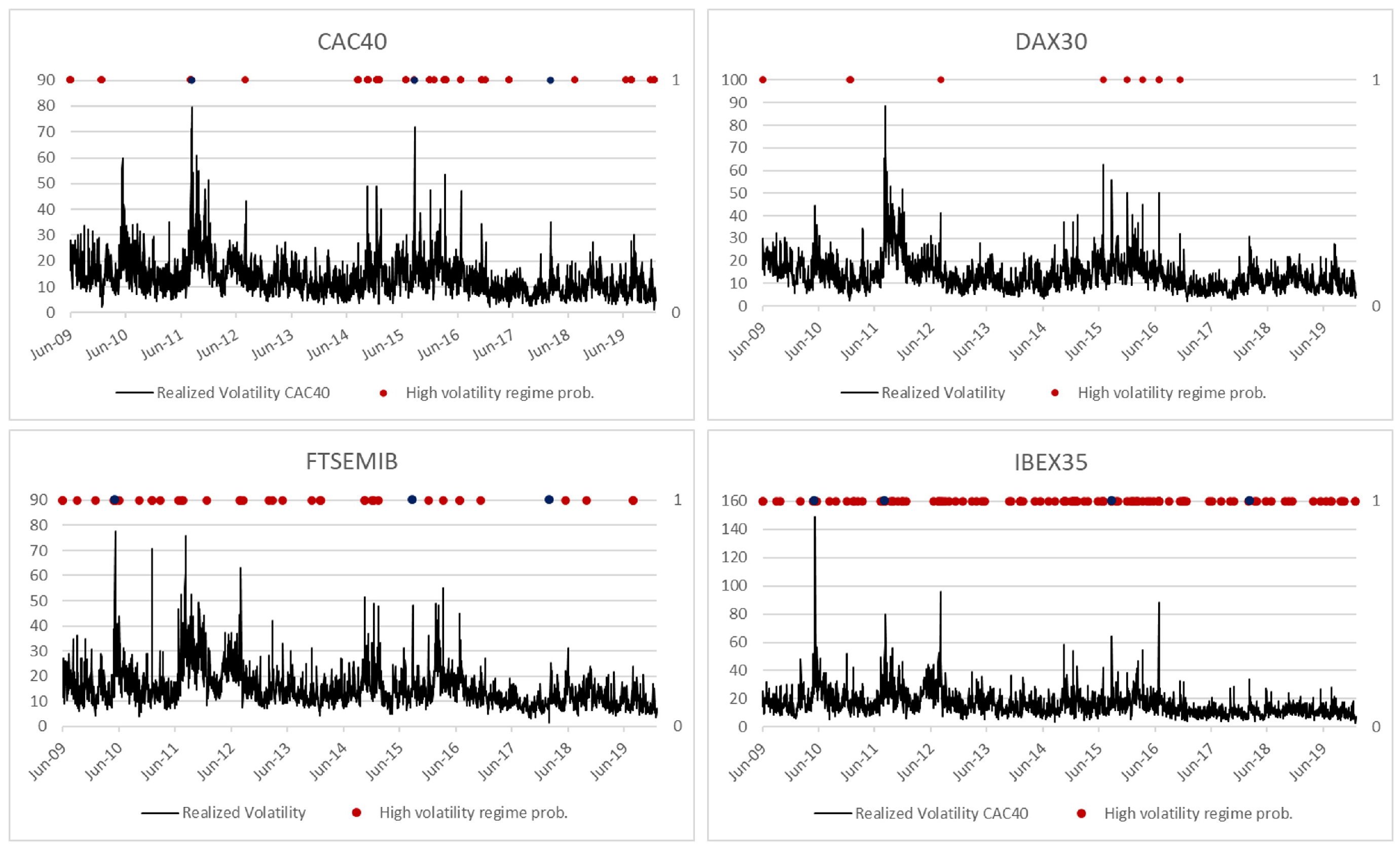
Generally, the analysis concerning volatility is carried out within the GARCH framework (Bollerslev 1986); however, in the last two decades, the new frontier in modeling volatility (due to the availability of ultra high frequency data) is represented by the class of Multiplicative Error Model, as introduced by Engle (2002) and revised by Engle and Gallo (2006) to account for asymmetry (Asymmetric MEM, AMEM). The idea behind the AMEM is quite straightforward: since volatility is a non-negative process, it could be modeled as the product of two positive time-varying factors, ${\mu }_t$, representing the conditional expectation (following a GARCH-type model) and ${ϵ}_t$, which is a positive random variable representing the error term. Given this specification, we can ensure the positiveness of our process without resorting to logs, thus modeling volatility directly, not the log of volatility. The MEM is usually expressed as Equation (1):

$$\begin{array}{c}{x}_t={\mu }_t{ϵ}_t,{ϵ}_t|{\Psi }_{t-1}\sim Gamma(\vartheta ,\frac{1}{\vartheta })\hfill \\ {\mu }_t=\omega +\alpha x_{t-1}+\beta {\mu }_{t-1}\hfill \end{array}$$

(1)

where ${\Psi }_t$ is the information set available at time t. In the MEM, the usual GARCH constraints to ensure positiveness and stationarity of the process are imposed, i.e., $\omega >0,\alpha \ge 0,\beta \ge 0,\gamma \ge 0$ and $(\alpha +\beta +\frac{\gamma }{2})<1$. As regards the error term, it follows a Gamma distribution depending only on one parameter, $\theta$;6 it can be derived that, in the MEM framework, both the conditional mean as well as the conditional variance of the dependent variable are time-varying and equal to ${\mu }_t$ and $\frac{{\mu }_t^2}{\theta }$, respectively.

Among the several extensions of the MEM (see, among others, Brownlees et al. 2011, 2012; Otranto 2015), Gallo and Otranto (2015) provide the Markov switching extension in order to account for several and frequent shifts in the average level and different dynamics of the volatility. In detail, their model, the MS-AMEM, is defined as in Equation (2):

$$\begin{array}{c}\hfill \begin{array}{c}{x}_t={\mu }_{t,s_t}{ϵ}_t,{ϵ}_t|{\Psi }_{t-1}\sim Gamma({\theta }_{s_t},1/{\theta }_{s_t})\hfill \\ {\displaystyle {\mu }_{t,s_t}=\omega +\sum _{i=1}^n{k}_i{I}_{s_t}+{\alpha }_{s_t}{x}_{t-1}+{\beta }_{s_t}{\mu }_{t-1,s_{t-1}}+{\gamma }_{s_t}{D}_{t-1}{x}_{t-1}}\hfill \end{array}\end{array}$$

(2)

where $I_{s_t}$ is a discrete dichotomic latent variable equals to 1 if $s_t\le i$ and 0 otherwise, while $k_i\ge 0$ for $i=2\dots n$ and $k_1=0$; it follows that the constant in regime j is equal to ${\displaystyle \omega +\sum _{i=1}^j{k}_i}$, and it increases passing from the lower to the higher regime. Therefore, $s_t$ represents the regime at time t and follows a first order Markov chain.

$$Pr(s_t=j|s_{t-1}=i,s_{t-2}\dots )=Pr(s_t=j|s_{t-1}=i)=p_{ij}$$

Positiveness and stationarity conditions do not change with respect to the simpler AMEM even if they are now state-dependent, i.e., ${\displaystyle \omega ,\sum _{i=1}^n{k}_i,{\alpha }_{s_t},{\beta }_{s_t},{\gamma }_{s_t}>0}$ and $0<{\alpha }_{s_t}+{\beta }_{s_t}+{\gamma }_{s_t}/2<1$,7 respectively, whereas the unconditional mean in state j is given by

$${\mu }_j=\frac{{\displaystyle \omega +\sum _{i=1}^j{k}_i}}{1-{\alpha }_j-{\beta }_j-{\gamma }_j/2}$$

3.1. The MS-AMEMX

Starting from the MS-AMEM, we augment Equation (2) to make it suitable for an analysis of spillover effects. In particular, our model is specified as Equation (3):

$$\begin{array}{cc}\hfill R{V}_t& ={\mu }_{t,s_t}{ϵ}_t,{ϵ}_t|{\Psi }_{t-1}\sim Gamma({\theta }_{s_t},1/{\theta }_{s_t})\hfill \\ \hfill {\mu }_{t,s_t}& =\omega +\alpha R{V}_{t-1}+\beta {\mu }_{t-1,s_{t-1}}+\gamma D_{t-1}R{V}_{t-1}+{\rho }_{s_t}R{V}_{t-1}^{S\&P500}+\hfill \\ \hfill & +\delta (E\left(x_t\right|{\Psi }_{t-1})-\overline{x})+\phi ({\Delta }_t-\overline{\Delta })\hfill \end{array}$$

(3)

In our model (call it MS-AMEMX), ${\mu }_t$ follows a GJR–GARCH8 (Glosten et al. 1993), which accounts for the asymmetric effect of returns on volatility ($D_{t-1}$ is equal to 1 if the return of the considered market at time $t-1$ is negative, 0 otherwise) with three exogenous variables: more in detail, we consider the $R{V}_{t-1}^{S\&P500}$, on the one hand, and two different proxies for the implementation ($E\left[x_t\right|{\Psi }_{t-1}]$) and the announcement (${\Delta }_t$)’s effects of the ECB unconventional policies, on the other. In other words, in our model, the $\rho$ coefficient is subject to regime changes (${\rho }_0$ and ${\rho }_1$ in the low and the high volatility regime, respectively), so that $R{V}^{S\&P500}$ is the variable driving the Eurozone volatility passing from the low- to the high-volatility regime and vice versa. Moreover, following Lacava et al. (2020), we proxy for the implementation effect by considering the amount of securities held for unconventional policy purposes as a fraction of the ECB total asset (UMP/TA), while we proxy for the announcement effect via a dummy variable taking value of 1 on monetary policy announcement days, 0 otherwise. The timing of these exogenous variables deserves particular attention. Because of the 6 h time difference (5 h during daylight saving time) between the New York Stock Exchange (NYSE) and the EU stock markets (i.e., trades in the US stock market occur mainly when the EU stock markets are closed), we consider $R{V}^{S\&P500}$ at time $t-1$. For what concerns the unconventional monetary policy proxies, because of the Efficient Market Hypothesis, we should consider them at time t, by accounting for the market expectations. However, since monetary policy announcements are regularly scheduled, we can consider the current value of the dummy variable, ${\Delta }_t$; finally, from preliminary analysis it emerges how UMP/TA follows a random walk process, so that we may measure market expectations on this variable by means of its own lagged value.

Therefore, through Equation (3), we aim to analyze whether and to what extent volatility shocks in the US market spill over into the European markets (i.e., we expect a positive and significant ${\rho }_{s_t}$ coefficients) and whether—through the unconventional monetary policy—the ECB was able to shield the Eurozone markets from these spillover effects (the $\delta$ coefficient is expected to be negative).

Regarding the statistical properties of our model, the stationarity condition does not change with respect to the MS-AMEM; conversely, since in our model only the unconventional policy proxies are the net of their own average value (their sample mean, $\overline{x}$ and $\overline{\Delta }$ for the implementation and the announcement effect, respectively), what changes is the unconditional mean, which is still regime-dependent but it is now equal to

$${\mu }_j=\frac{\omega +{\rho }_j{\overline{RV}}^{S\&P500}}{1-\alpha -\beta -\gamma /2}$$

where ${\overline{RV}}^{S\&P500}$ is the unconditional expected value of the S&P500 Realized Volatility.

As usual, in the Markov-switching framework, we estimate the model in Equation (3) by means of the Hamilton filter and smoother (Hamilton 1994, chp. 22) by adopting the solution proposed by Kim (1994) to solve the well-known path dependence problem: in particular, given the dependence of ${\mu }_t$ on all the past values of $s_t$, it is necessary to track all the possible paths of the regime between the first and the last observation. The Kim’s solution consists in collapsing—after each step of the Hamilton filter—the four possible values of ${\mu }_t$ into two values, via a weighted average at time $t-1$.

$${\mu }_{t,s_t}=\frac{{\displaystyle \sum _{i=1}^{n}Pr[s_{t-1}=i,s_t=j|{\Psi }_t]{\mu }_{t,s_{t-1},s_t}}}{Pr[s_t=j|{\Psi }_t]}$$

As a by-product of the Hamilton filter, we obtain the Quasi-likelihood function, so that the estimator is consistent and efficient, regardless of whether the gamma distribution is appropriate for the error term (Engle and Gallo 2006); relying, on the QMLE, we compute robust standard errors (in the sandwich form, White 1982), to shield against the shape parameter of the Gamma distribution.

4. Empirical Application

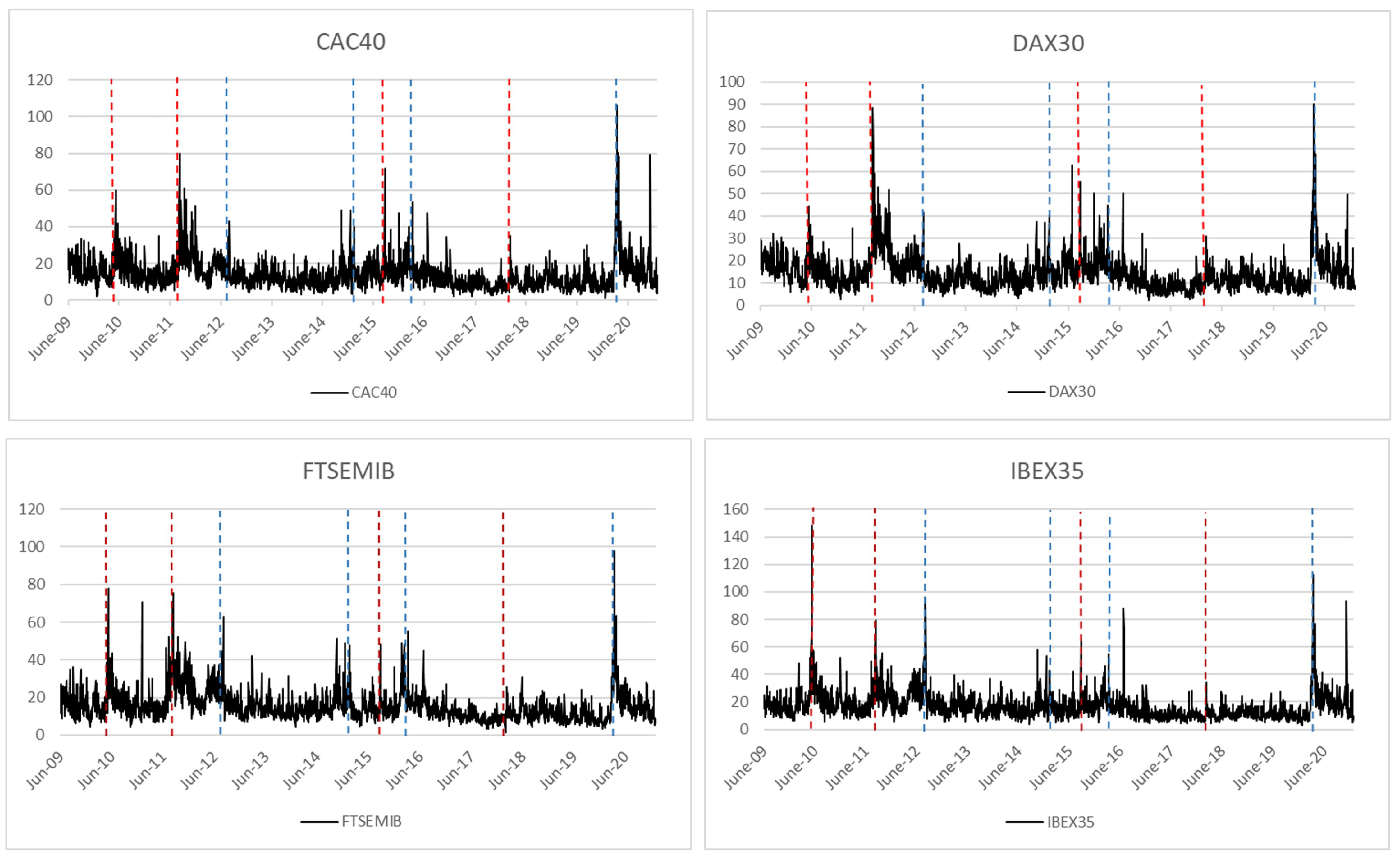
This section is devoted to the presentation of estimation results. Specifically, Section 4.1 presents the description of our dataset, with the descriptive statistics provided in

Table 1. Descriptive statistics for CAC40, DAX30, FTSEMIB, IBEX35 Realized Volatility. Sample period: 1 June 2009 to 31 December 2020.

	CAC40	DAX30	FTSEMIB	IBEX35
Mean	14.16	14.369	15.569	17.024
Min	1.102	2.141	1.578	2.974
Max	106.37	89.92	97.699	148.61
St.Dev.	8.616	8.031	8.243	9.768
Skewness	3.106	2.761	2.458	3.379
Kurtosis	18.797	14.823	11.432	24.285
N. observations	2882	2853	2857	2877

.

Estimation results are discussed in Section 4.2, together with residual diagnostics and a first comparison—based both on Information Criteria (AIC and BIC) as well as on the in-sample forecasting capability (via MSE and QLike)—of our models with respect to the competitive ones.

Finally, in Section 4.3 we compare the out-of-sample forecasting performance of the considered models through the Diebold–Mariano test (Diebold and Mariano 1995).

4.1. The Dataset

In our empirical analysis, we employ a dataset consisting of daily observations of the Realized kernel Volatility (RV hereafter) of four Eurozone stock indices (CAC40, DAX30, FTSEMIB and IBEX35), which is a robust estimator of volatility with respect to microstructure noise (Barndorff-Nielsen et al. 2008). We distinguish two different samples: the estimation period going from 1 June 2009 to 31 December 2019, and the forecasting period from 1 January 2020 to 31 December 2020, which is employed for the analysis in Section 4.3. Furthermore, we consider the RV of the S&P500 as a source of volatility spillovers, while we use the returns series of each considered stock index to construct the dummy variable that is used to account for the asymmetric effects of returns on volatility;9 finally, we complete our dataset with two proxies to measure the unconventional policy implementation and the announcement effects. As said, the former is measured by the ratio between the amount of securities held for unconventional policy purposes and the ECB total asset,10 whereas the latter is measured through a dummy variable taking a value of 1 on monetary policy announcement days and 0 otherwise.11

Figure 1 shows the evolution of our stock market indices. In all the cases, the series behave quite similarly to each other, with volatility remaining relatively low for long periods; for example, relevant high-volatility periods, common for all the series, correspond to the sovereign debt crisis (2010 and 2011) and to the COVID-19 pandemic in the last year of our sample. The possibility to distinctly observe periods of low and high volatility, together with the volatility clustering phenomenon, represents a crucial justification for the estimation of a model with regime changes.

In the same figure, the red dashed lines refer to some important dates, which affected the US stock market volatility, causing a volatility spike12 in the $R{V}^{S\&P500}$: for example, the flash crashes on 6 May 2010 and on 24 August 2015; the US debt downgrade on 8 August 2011; finally, on 6 February 2018, when the S&P500 detected the worst decrease since the 2011, probably due to the fear about an increment of the federal funds rate. In all cases, it seems that volatility spikes in the $R{V}^{S\&P500}$ propagated in the Eurozone, with a peak of volatility detected for all the considered stock markets. For what concerns the blue dashed lines, they represent some relevant unconventional policy-related dates, i.e., the “whatever it takes” declaration by the ECB then-President Draghi (on 26 July 2012), the EAPP announcements (on 22 January 2015), the increment of monthly purchases within the EAPP (on 10 March 2016), and the announcement of the PEPP (18 March 2020). In all the cases, it should be noticed how RV decreases after the announcements and remain low for long periods, giving an idea about the positive impact of unconventional policies on financial market stability. It is important to notice how, in the second half of the sample (starting from the 2016), volatility spikes are relatively small compared to spikes occurring on the first part of the sample; this would represent a first sign that unconventional policy—the amount of purchased securities, in particular—was also able to reduce the impact of international volatility spillovers.

Descriptive statistics are provided in Table 1. It emerges clearly the similar features between the CAC40 and DAX30 Realized Volatility series, which have a lower mean value than that of FTSEMIB and IBEX35. This represents well-expected results, since the latter countries, during the sample period, experienced a deeper recession, which contributed to create uncertainty among investors with a direct impact on financial markets. Moreover, the high index of kurtosis clearly reflects the well-known stylized fact of Realized Volatility, i.e., its unconditional distribution has fatter tails with respect to the Gaussian one. Finally, in all the series, there is a high difference between the minimum and the maximum value, which gives us a further justification for the adoption of a Markov switching model.

As regards the monetary policy dummy variable, since it is not possible to know in advance whether an announcement concerns conventional or unconventional policy, both the categories are considered in constructing our dummy variable, which consists of 153 announcements. Not surprisingly, important dates correspond to the announcements of the most important unconventional policy programs, such as: the Security Market Programme (SMP, referring to the purchases of government bond), the Outright Monetary Transaction (OMT), the Expanded Asset Purchase Programme (EAPP, concerning both private and public bond), and the Pandemic Emergency Purchase Programme (PEPP, to sustain the EU economy during the ongoing COVID-19 pandemic).

Finally, Figure 2 shows the evolution of the ECB balance sheet composition. In detail, the unconventional policy weight remains relatively low with the implementation of the CBPP1, the SMP, and the OMT (period 2009–2014), while it assumes a leading role with the EAPP implementation starting from 2015. In the period 2015–2020, unconventional monetary policy is worth about the 50% of the ECB total asset, on average, while it is just the 6%, on average, in the period 2009–2014. Furthermore, within the EAPP, the greatest share of purchases (73%) refers to the PSPP, while the CSPP accounts only for the 4% of the total amount; the monthly purchases are reduced in 2019 when no APP was implemented; finally, it increases again in the last year of the sample with the adoption of the PEPP.

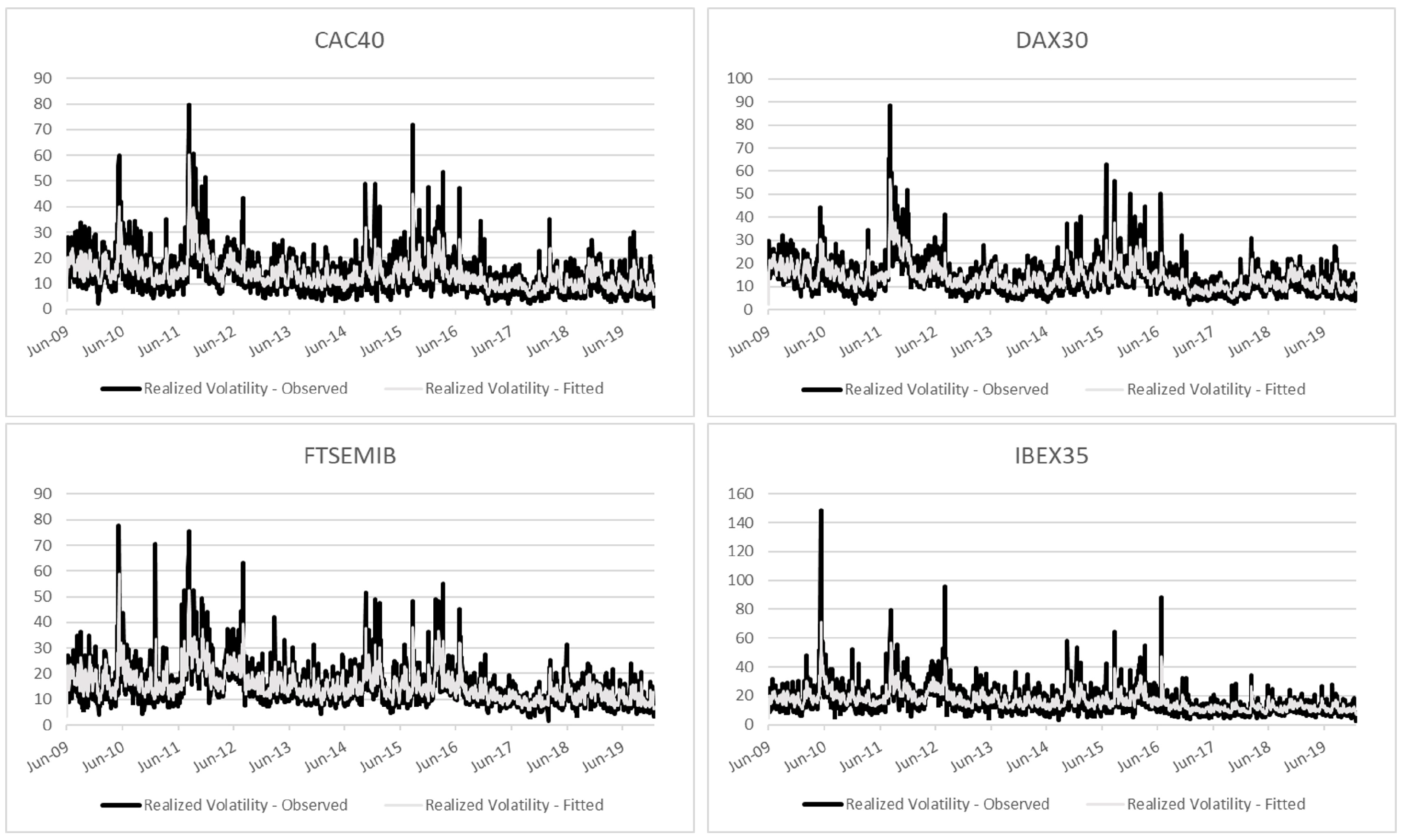
4.2. Estimation Results

In this subsection, the estimation results of our empirical analysis are discussed. In particular,

Table 2. Model Estimation results from the AMEM (robust s.e. in parenthesis) and p-values for the Ljung–Box statistics. Estimation period: 1 June 2009–31 December 2019. Dependent Variable: Realized Volatility.

	CAC40	DAX30	FTSEMIB	IBEX35
$\omega$	0.920	0.957	1.224	1.092
	(0.198)	(0.249)	(0.291)	(0.243)
$\alpha$	0.188	0.119	0.286	0.236
	(0.026)	(0.225)	(0.028)	(0.028)
$\beta$	0.69	0.693	0.594	0.662
	(0.032)	(0.024)	(0.035)	(0.034)
$\gamma$	0.104	0.092	0.074	0.066
	(0.013)	(0.011)	(0.011)	(0.012)
$\theta$	7.474	9.795	10.807	9.113
	(0.256)	(0.542)	(0.509)	(0.342)
p-values for Ljung-Box statistics
Ljung–Box 1	0.019	0.053	0.105	0.002
Ljung–Box 5	0.08	0.023	0.723	0.017
Ljung–Box 10	0.118	0.008	0.871	0.102

shows results of the AMEM, while

Table 3. Model Estimation results from the AMEMX (robust s.e. in parenthesis) and p-values for the Ljung–Box statistics. Estimation period: 1 June 2009–31 December 2019. Dependent Variable: Realized Volatility.

	CAC40	DAX30	FTSEMIB	IBEX35
$\omega$	1.358	1.136	1.876	1.739
	(0.264)	(0.294)	(0.37)	(0.232)
$\alpha$	0.156	0.178	0.286	0.215
	(0.024)	(0.022)	(0.025)	(0.028)
$\beta$	0.633	0.666	0.517	0.611
	(0.041)	(0.029)	(0.041)	(0.043)
$\gamma$	0.112	0.091	0.074	0.072
	(0.013)	(0.011)	(0.012)	(0.012)
$\rho$	0.069	0.036	0.052	0.047
	(0.018)	(0.013)	(0.014)	(0.014)
$\delta$	−0.853	−0.448	−1.337	−1.305
	(0.21)	(0.183)	(0.316)	(0.282)
$\phi$	1.48	1.104	2.228	2.042
	(0.453)	(0.373)	(0.493)	(0.494)
$\theta$	7.74	9.991	11.371	9.513
	(0.252)	(0.524)	(0.492)	(0.351)
p-values for Ljung-Box statistics
Ljung–Box 1	0.335	0.188	0.813	0.052
Ljung–Box 5	0.324	0.087	0.899	0.073
Ljung–Box 10	0.086	0.006	0.517	0.232

refers to the AMEM augmented with our proxies for the spillover effects and for unconventional policy.

Starting from the AMEM, all the coefficients are highly significant (at a 1% level). Regarding the constant $\omega$ it is higher in the high-debt countries (Italy and Spain) than in the low-debt ones (France and Germany), reflecting the higher risk in these countries during the sample period. The model is able to reproduce the persistence feature of volatility13 (ranging between $0.858$ and $0.931$ for the DAX30 and IBEX35, respectively), even though it suffers from residual autocorrelation, as shown from the Ljung–Box statistics reported in the bottom of the same table. In detail, we fail to reject the null of non-autocorrelated residuals in three out of four cases, i.e., CAC40 (for lag 10) and IBEX35 (lags 1 and 5), DAX30 (at every considered lag).

The significance of the estimated parameters does not change when we account for the spillover and the unconventional policy effects. As shown in Table 3, even the exogenous variables are significant at a 1% level, and they enter the model with the expected sign. In particular, $\rho$ is positive, meaning that a shock of volatility in the US market spills over to the Eurozone markets with a similar magnitude for all the considered indices. Not surprisingly, a difference between low-debt and high-debt countries exists for the unconventional policy effects, with both the announcement and the implementation effect being higher in the case of FTSEMIB and IBEX35. In line with other researches, $\phi$ is positive (e.g., Bomfim 2003; Chan and Gray 2018; Lacava et al. 2020; Shogbuyi and Steeley 2017), whereas $\delta$ is negative (see, among others, Eser and Schwaab 2016; Fratzscher et al. 2016; Ghysels et al. 2017; Lacava et al. 2020). This leads to the first important result that volatility decreased because of the unconventional policy implementation, even if it increased on monetary policy announcement days.

Despite the significance of all the parameters, this model also suffers from mis-specification, since residuals are still autocorrelated at a 10% level (at least) in the case of CAC40, DAX30 and IBEX35.

Table 4. Model Estimation results from the MS-AMEMX (robust s.e. in parenthesis) and p-values for the Ljung–Box statistics. Estimation period: 1 June 2009–31 December 2019. Dependent Variable: realized volatility.

	CAC40	DAX30	FTSEMIB	IBEX35
$\omega$	1.103	0.705	1.436	1.396
	(0.184)	(0.109)	(0.239)	(0.242)
$\alpha$	0.139	0.172	0.279	0.155
	(0.02)	(0.018)	(0.025)	(0.029)
$\beta$	0.677	0.701	0.551	0.689
	(0.037)	(0.027)	(0.04)	(0.041)
$\gamma$	0.113	0.088	0.069	0.073
	(0.011)	(0.008)	(0.01)	(0.009)
${\rho }_0$	0.047	0.038	0.043	0.01
	(0.016)	(0.011)	(0.014)	(0.019)
${\rho }_1$	0.182	0.278	0.214	0.241
	(0.11)	(0.119)	(0.081)	(0.069)
$\delta$	−0.737	−0.251	−0.948	−1.047
	(0.158)	(0.102)	(0.206)	(0.209)
$\phi$	1.061	0.641	1.717	1.342
	(0.387)	(0.305)	(0.398)	(0.374)
${\theta }_0$	9.14	11.288	14.406	13.228
	(0.513)	(0.429)	(1.338)	(1.105)
${\theta }_1$	2.879	0.769	3.124	8.403
	(0.909)	(0.785)	(1.888)	(1.259)
$p_{00}$	0.969	0.994	0.955	0.844
	(0.032)	(0.005)	(0.038)	(0.086)
$p_{11}$	0.583	0.286	0.33	0.252
	(0.381)	(0.238)	(0.201)	(0.154)
p-values for Ljung-Box statistics
Ljung–Box 1	0.417	0.529	0.875	0.004
Ljung–Box 5	0.369	0.977	0.855	0.015
Ljung–Box 10	0.424	0.994	0.977	0.127

shows estimation results from the MS-AMEMX, which represents the main focus of this paper. Focusing on the parameters of interest, we still have a higher unconventional policy effects for the FTSEMIB and IBEX35, whereas the spillover effects seem to hit all the indices in a similar way. More importantly, the $\rho$ coefficient is significant in both the volatility regimes, corroborating our idea of time-varying spillover effects. Specifically, ${\rho }_0$ is highly significant but close to zero in all the cases; in the high volatility regime, instead, the $\rho$ coefficient increases remarkably and it ranges between 0.182 and 0.278 for the CAC40 and DAX30, respectively. Of course, it represents evidence in favor of the view of higher financial markets integration during high-volatility periods. For what concerns regime probabilities, there is a higher probability of remaining in regime 0 (low volatility), which has an average duration, given by $\frac{1}{1-p_{00}}$, between 6 and 116 business days for the IBEX35 and DAX30, respectively; as expected, the high volatility regime is short-lived, with a higher average duration of 2 business days for the case of CAC40 (1 day for the other indices). This is shown in Figure 3, in which we compare the observed RV series (black line) with the high-volatility regime probability (represented by the red dots and measured in the right axis). With the only exception of the DAX30, in three out of four cases, the high-volatility regime is the prevalent regime in correspondence with volatility spikes; importantly, for these indices, the process is in the high regime on days of the flash crashes of the US stock market but also on days when bad news for the US economy occurs (some examples are represented by the blue dots in the figure). Therefore, it allows us to conclude that the presented model correctly detects volatility spillovers from the US to the Eurozone financial markets.

Furthermore, even the $\theta$ coefficients are coherent with the definition of the two volatility regimes: ${\theta }_1$ is always lower than ${\theta }_0$, meaning that residuals have a higher dispersion in the high volatility regime with respect to the regime of low volatility.

Finally, this specification correctly captures the autoregressive structure of volatility in three out of four cases; i.e., we cannot reject the null of residual autocorrelation at a 1% level only in the case of IBEX35 at lag 1.

Considering the opposite sign of coefficients ${\rho }_{s_t}$ and $\delta$, with the purpose of highlighting the joint effect of spillovers and unconventional policy implementation, in

Table 5. (a) Spillover effect $({\rho }_{s_t}·R{V}_t^{S\&P500})$, (b) unconventional policy effect $(\delta ·{\frac{UMP}{TA}}_t)$ and (c) net effect (a,b) from the MS-AMEMX.

(a)	Spillover Effect
	Full Sample	Sub-Sample	Sub-Sample
		2009–2014	2015–2019
CAC40	0.542	1.105	0.452
DAX30	0.412	0.574	0.469
FTSEMIB	0.5	0.844	0.507
IBEX35	0.268	0.46	0.475
(b)	Unconventional Policy Effect
	Full Sample	Sub-Sample	Sub-Sample
		2009–2014	2015–2019
CAC40	−0.212	−0.12	−1.248
DAX30	−0.072	−0.002	−0.852
FTSEMIB	−0.273	0.003	−0.934
IBEX35	−0.301	−0.121	−1.53
(c)	Net Effect
	Full Sample	Sub-Sample	Sub-Sample
		2009–2014	2015–2019
CAC40	0.33	0.985	−0.795
DAX30	0.34	0.572	−0.383
FTSEMIB	0.227	0.841	−0.428
IBEX35	−0.033	0.339	−1.055

, we show the average difference between $({\rho }_{s_t}·R{V}_t^{S\&P500})$ and $(\delta ·{\frac{UMP}{TA}}_t)$. As regards the spillover effects, because of the state dependence of the ${\rho }_{st}$ coefficients, we consider either ${\rho }_0$ or ${\rho }_1$ based on the value of the smoothed probabilities:14 more in detail, the spillover effect is given by $({\rho }_0·R{V}_t^{S\&P500})$ when the smoothed probability, $p_{0,t|T}>0.5$, while it is equal to $({\rho }_1·R{V}_t^{S\&P500})$ when $p_{1,t|T}>0.5$.

Focusing on the full estimation period (2009–2019, column 1), it is possible to notice how the spillover effects predominate in three out of four cases (section c of the table): despite the mitigating effect of unconventional policies on stock market volatility, during the whole sample period, there was an increase in volatility, ceteris paribus, between 0.227 and 0.34 for the FTSEMIB and CAC40, respectively. However, in this kind of analysis, it should be kept in mind that the amount of monthly purchases under the various APPs was not constant over time; in fact, as shown in Figure 2, the amount of purchased securities increased remarkably starting from the 2015. Mainly for this reason, the same table (columns 2 and 3) shows results for the sub-samples 2009–2014 and 2015–2019 (before and after the announcement of the EAPP).15 What emerges is the crucial role played by the EAPP in reducing stock market volatility. In particular, while we observe an average increment in volatility because of the spillover effects in the first sub-sample (section c, column 2), the EAPP makes the difference with a volatility average reduction between −0.383 (in the case of the DAX30) and −1.055 (IBEX35), respectively. Importantly, even though it could be reasonably argued that volatility spillovers decrease passing from the first to the second sub-sample (section a of Table 5), it is likewise important to stress how the size of the unconventional policy effect changes across sub-samples: as shown in section b, the reduction of volatility due to the implementation of unconventional policy is between −0.002 and −0.012 in the period 2009–2014, while in the period 2015–2019, we observe a higher average reduction in all the cases, that is between −0.852 (DAX30) and −1.53 (IBEX35). In conclusion, while volatility increases due to the spillover effects from the US market, the ECB was able to preserve confidence in financial markets through an overall reduction in volatility brought about by the various asset purchase programs. This is, perhaps, the most important result of this analysis, stating that the amount of purchased securities is crucial for a dampening effect of unconventional policy on volatility. Considering that our proxy measures the weight of unconventional policy in the ECB balance sheet, this result is in line with Curdia and Woodford (2011), who find that what matters for the effectiveness of such policies is the balance sheet composition rather than its size.16 In other words, this result suggests us how policies that cause a change in the central bank’s balance sheet composition (i.e., the kind of policy that the ECB has been establishing since 2015) could be used as a monetary tool to reduce volatility and preserve financial stability even from foreign market shocks.

Finally,

Table 6. Models comparison (best model in bold) through the Information Criteria (AIC and BIC) and forecasting capability (MSE and QLike loss functions). Sample period: 1 June 2009–31 December 2019.

	CAC40			DAX30
	AMEM	AMEMX	MS-AMEMX	AMEM	AMEMX	MS-AMEMX
LogLik	−7712.012	−7663.943	−7627.295	−7365.365	−7338.932	−7254.689
AIC	5.853	5.819	5.794	5.643	5.626	5.564
BIC	5.864	5.837	5.821	5.655	5.643	5.591
MSE	30.357	29.222	29.481	23.847	23.352	23.17
QLIKe	0.068	0.066	0.066	0.052	0.051	0.052
	FTSEMIB			IBEX35
	AMEM	AMEMX	MS-AMEMX	AMEM	AMEMX	MS-AMEMX
LogLik	−7514.834	−7446.347	−7373.76	−7970.565	−7911.763	−7860.52
AIC	5.749	5.699	5.647	6.065	6.023	5.987
BIC	5.76	5.717	5.674	6.076	6.041	6.014
MSE	28.327	27.47	27.817	42.957	41.452	41.859
QLIKe	0.047	0.045	0.045	0.056	0.053	0.054

compares the in-sample performance of the estimated models by considering both the Information Criteria (AIC and BIC) and the forecasting power of the models (Mean squared error (MSE) and Quasi Likelihood (QLike)). In sum, as a primary focus on Information Criteria, the results show better fitting properties of our model with respect to the competitive ones (the best model in bold) for all the indices. Conversely, the MS-AMEMX is not as good as the time-invariant parameters model relatively to the forecasting performance: Table 6 shows a higher forecasting capability of the AMEMX, even though the MS-AMEMX performs similarly when we look at the QLike loss function. The good fitting properties of our model are also shown in Figure 4, which depicts both the observed ($R{V}_t$, black line) and the fitted (${\mu }_t$, gray line) volatility series: for all the considered indices, ${\mu }_t$ follows the same path of the observed series, and it jumps on the same days on which volatility spikes are observed also for the RV series.

We remand to the next subsection for a further models comparison, based on the out-of-sample forecasting performance of the considered models.

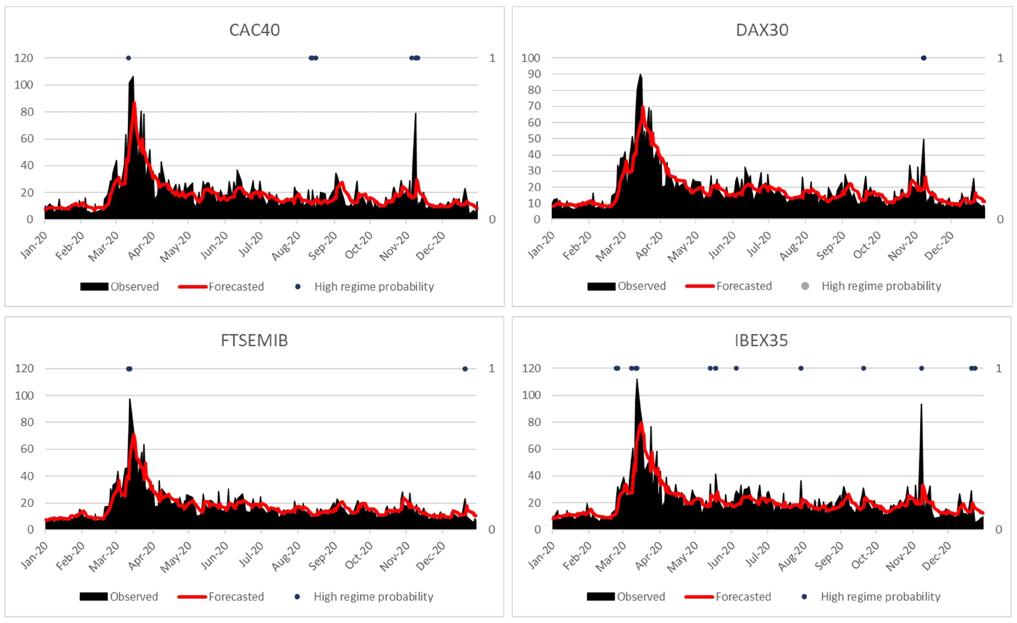
4.3. Out-of-Sample Analysis

In this section, we perform an out-of-sample analysis, which is suitable for a further comparison of the considered models. In doing so, we rely on the Diebold–Mariano (one-tailed) test (Diebold and Mariano 1995) for the comparison of the forecasting accuracy of two alternative models. In particular, the null hypothesis that two models have the same forecasting power is tested (based on the MSE loss function—which is consistent, as shown by Patton 2011) against the alternative hypothesis that the second model outperforms the first one.

For this purpose, we have considered the period between June 2009 and December 2019 as the estimation period, whereas the forecasting period refers to 2020. The t-statistics and p-values of the Diebold–Mariano test are shown in

Table 7. t-statistics and p-value of the Diebold–Mariano test. $H_0:$ MSE (model 1) = MSE (model 2); $H_a:$ MSE (model 1) < MSE (model 2). In bold, p-values < 0.1. Sample period: 1 June 2009–31 December 2019. Forecasting period: 1 January 2020 to 31 December 2020.

	CAC40		DAX30
Model 1/Model 2	t-Statistics	p-Value	t-Statistics	p-Value
AMEM/AMEMX	1.999	0.023	1.792	0.037
AMEM/MS-AMEMX	1.349	0.089	0.846	0.199
AMEMX/MS-AMEMX	0.307	0.379	-0.035	0.514
	FTSEMIB		IBEX35
Model 1/Model 2	t-Statistics	p-Value	t-Statistics	p-Value
AMEM/AMEMX	1.548	0.062	2.233	0.013
AMEM/MS-AMEMX	1.355	0.088	1.328	0.093
AMEMX/MS-AMEMX	0.967	0.167	0.752	0.226

. Not surprisingly, there are no differences between the forecasting capability of the AMEMX and MS-AMEMX: this result is in line with the branch of literature stating that non-linear models have better in-sample properties, while they perform poorly in the out-of-sample context (see, among others, Diebold and Nason 1990; Hansen 2010).

Importantly, the AMEM is the worst model when compared to both the AMEMX and MS-AMEMX (we always reject the null hypothesis, values in bold), representing further evidence that spillovers of volatility and unconventional policies represent important determinants for the forecasting of the Eurozone volatility.

Crucially, both the observed RV and the series forecasted through our MS-AMEMX follow a similar path also in the out-of-sample period: as shown in Figure 5, the forecasted volatility (red line) is able to reproduce the non-linear features that characterize the observed RV series (black area). The same figure also shows the probability of being in the high regime (blue points); briefly, for all the indices, it is evident how the model is able to reproduce the volatility spikes observed in March—with an increasing uncertainty due to the outbreak of the COVID-19 pandemic—or (to a lesser extent) in November, with the onset of the second wave of COVID-19.

5. Concluding Remarks

In this paper, we analyzed whether the ECB’s unconventional policies served as a shield against volatility spillovers from the US stock market. While most of the research focuses on the impact of unconventional policies on the real economy as well as on bond and stock market returns and volatility, the literature concerning the relationship between unconventional monetary policy and exogenous shocks from foreign markets is still narrow. We contribute to this branch of literature by proposing an extension of the MS-AMEM in which the impact of volatility spillovers from the S&P500 on Eurozone markets depends on whether the process is in the low- or in the high-volatility regime. Differently from other analyses concerning the effect of unconventional policies on foreign markets, in this research, we account for the joint effect of unconventional policy and volatility spillovers. In detail, our MS-AMEMX shows how, despite volatility spillovers significantly increasing volatility of the considered stock indices, the ECB was able to reduce volatility via unconventional monetary policy in both the low- and high-volatility regimes. Moreover, by looking at the difference between low-debt and high-debt countries, while spillover effects impacted the considered countries’ indices in a similar way, it seems that high-debt countries benefited more from the implementation of these extraordinary measures. Furthermore, by reproducing the same analysis on two sub-samples, we find how the EAPP played a leading role in preserving financial stability, meaning that the amount of purchased securities is actually crucial for unconventional monetary policy to be effective.

In addition, the out-of-sample analysis corroborates the validity of our model specification even for forecasting purposes.

This work would contribute to the current debate about the impact of ECB’s unconventional monetary policy on the Eurozone financial stability. In particular, it could provide important information for policy makers about the suitability of this kind of policy as a tool to preserve financial stability. Furthermore, it could also help investors in the asset portfolio construction process. As regards this last aspect, as an extension of this research, it would be interesting to reproduce this analysis within the multivariate framework, so that it could be possible to capture potential interdependence across stock indices. In other words, the multivariate extension of our model could represent an interesting starting point to build an efficient portfolio allocation strategy, in particular, if a set of securities is taken into consideration in place of stock indices. This goal could be achieved by combining our model together with existing strategies of asset allocation, which are based on the network approach (see, among others, Giudici et al. 2020; Pagnottoni 2019; Peralta and Zareei 2016; Pichler et al. 2021), so that accounting for a time-varying spillover effects (within the MS framework) could improve the estimation of the covariance matrix.

Finally, the robustness of our results could be further tested by considering other non-parametric volatility proxies (e.g., the daily range, computed as the difference between the highest and the lowest recorded value in a day), which would also give us the opportunity to broaden the analysis to other stock market indices, for which RV is not available yet.

References

1. Altavilla, Carlo, Domenico Giannone, and Michele Lenza. 2014. The Financial and Macroeconomic Effects of OMT. announcements. ECB Working Paper No. 1707. Rome: European Central Bank. [Google Scholar]
2. Apostolou, Apostolos, and John Beirne. 2017. Volatility Spillovers of Federal Reserve and ECB Balance Sheet Expansions to Emerging Market Economies. ECB Working Paper No. 2044. Rome: European Central Bank. [Google Scholar]
3. Baele, Lieven. 2005. Volatility spillover effects in european equity markets. Journal of Financial and Quantitative Analysis 40: 373–401. [Google Scholar] [CrossRef] [Green Version]
4. Barndorff-Nielsen, Ole E., Peter Reinhard Hansen, Asger Lunde, and Neil Shephard. 2008. Designing realised kernels to measure the ex-post variation of equity prices in the presence of noise. Econometrica 76: 1481–536. [Google Scholar] [CrossRef] [Green Version]
5. Bollerslev, Tim. 1986. Generalized Autoregressive Conditional Heteroskedasticity. Journal of Econometrics 31: 307–27. [Google Scholar] [CrossRef] [Green Version]
6. Bomfim, Antulio N. 2003. Pre-announcement effects, news effects, and volatility: Monetary policy and the stock market. Journal of Banking & Finance 27: 133–51. [Google Scholar]
7. Brownlees, Christian T., Fabrizio Cipollini, and Giampiero M. Gallo. 2011. Intra-daily volume modeling and prediction for algorithmic trading. Journal of Financial Econometrics 9: 489–518. [Google Scholar] [CrossRef] [Green Version]
8. Brownlees, Christian T., Fabrizio Cipollini, and Giampiero M. Gallo. 2012. Multiplicative Error Models. In Volatility Models and Their Applications. Edited by Luc Bauwens, Christian M. Hafner and Sébastien Laurent. Hoboken: John Wiley & Sons, pp. 223–47. [Google Scholar]
9. Burriel, Pablo, and Alessandro Galesi. 2018. Uncovering the heterogeneous effects of ECB unconventional monetary policies across euro area countries. European Economic Review 101: 210–29. [Google Scholar] [CrossRef]
10. Chan, Kam F., and Philip Gray. 2018. Volatility jumps and macroeconomic news announcements. Journal of Futures Markets 38: 881–97. [Google Scholar] [CrossRef]
11. Chen, Han, Vasco Cúrdia, and Andrea Ferrero. 2012. The macroeconomic effects of large-scale asset purchase programmes. The Economic Journal 122: F289–F315. [Google Scholar] [CrossRef]
12. Ciarlone, Alessio, and Andrea Colabella. 2018. Asset Price Volatility in EU-6 Economies: How Large Is the Role Played by the ECB? Bank of Italy Temi di Discussione Working Paper No. 1175. Rome: Banca D’italia. [Google Scholar]
13. Curdia, Vasco, and Michael Woodford. 2011. The central-bank balance sheet as an instrument of monetary policy. Journal of Monetary Economics 58: 54–79. [Google Scholar] [CrossRef] [Green Version]
14. Diebold, Francis X., and Roberto S. Mariano. 1995. Comparing predictive accuracy. Journal of Business & Economic Statistics 13: 253–63. [Google Scholar]
15. Diebold, Francis X., and James A. Nason. 1990. Nonparametric exchange rate prediction? Journal of International Economics 28: 315–32. [Google Scholar] [CrossRef]
16. Diebold, Francis X., and Kamil Yilmaz. 2009. Measuring financial asset return and volatility spillovers, with application to global equity markets. The Economic Journal 119: 158–71. [Google Scholar] [CrossRef] [Green Version]
17. Diebold, Francis X., and Kamil Yilmaz. 2012. Better to give than to receive: Predictive directional measurement of volatility spillovers. International Journal of Forecasting 28: 57–66. [Google Scholar] [CrossRef] [Green Version]
18. Diebold, Francis X., and Kamil Yılmaz. 2014. On the network topology of variance decompositions: Measuring the connectedness of financial firms. Journal of Econometrics 182: 119–34. [Google Scholar] [CrossRef] [Green Version]
19. Edwards, Sebastian. 1998. Interest rate volatility, contagion and convergence: An empirical investigation of the cases of Argentina, Chile and Mexico. Journal of Applied Economics 1: 55–86. [Google Scholar] [CrossRef] [Green Version]
20. Edwards, Sebastian, and Raul Susmel. 2001. Volatility dependence and contagion in emerging equity markets. Journal of Development Economics 66: 505–32. [Google Scholar] [CrossRef] [Green Version]
21. Edwards, Sebastian, and Raul Susmel. 2003. Interest-rate volatility in emerging markets. Review of Economics and Statistics 85: 328–48. [Google Scholar] [CrossRef]
22. Engle, Robert F. 2002. New frontiers for ARCH models. Journal of Applied Econometrics 17: 425–46. [Google Scholar] [CrossRef] [Green Version]
23. Engle, Robert F., and Giampiero M. Gallo. 2006. A multiple indicators model for volatility using intra-daily data. Journal of Econometrics 131: 3–27. [Google Scholar] [CrossRef] [Green Version]
24. Engle, Robert F., Giampiero M. Gallo, and Margherita Velucchi. 2012. Volatility spillovers in East Asian financial markets: A MEM based approach. Review of Economics and Statistics 94: 222–33. [Google Scholar] [CrossRef]
25. Engle, Robert F., Takatoshi Ito, and Wen-Ling Lin. 1990. Meteor showers or heat waves?: Heteroskedastic intra daily volatility in the foreign exchange market. Econometrica 58: 1749–78. [Google Scholar] [CrossRef]
26. Eser, Fabian, and Bernd Schwaab. 2016. Evaluating the impact of unconventional monetary policy measures: Empirical evidence from the ECB’s securities markets programme. Journal of Financial Economics 119: 147–67. [Google Scholar] [CrossRef]
27. Forbes, Kristin J., and Roberto Rigobon. 2002. No contagion, only interdependence: Measuring stock market comovements. The Journal of Finance 57: 2223–61. [Google Scholar] [CrossRef]
28. Francq, Christian, Michel Roussignol, and Jean-Michel Zakoïan. 2001. Conditional heteroskedasticity driven by hidden Markov chains. Journal of Time Series Analysis 22: 197–220. [Google Scholar] [CrossRef]
29. Fratzscher, Marcel, Marco Lo Duca, and Roland Straub. 2016. ECB unconventional monetary policy: Market impact and international spillovers. IMF Economic Review 64: 36–74. [Google Scholar] [CrossRef]
30. Gallo, Giampiero M., and Edoardo Otranto. 2008. Volatility spillovers, interdependence and comovements: A Markov switching approach. Computational Statistics & Data Analysis 52: 3011–26. [Google Scholar] [CrossRef] [Green Version]
31. Gallo, Giampiero M., and Edoardo Otranto. 2015. Forecasting realized volatility with changing average levels. International Journal of Forecasting 31: 620–34. [Google Scholar] [CrossRef]
32. Gallo, Giampiero M., and Edoardo Otranto. 2018. Combining sharp and smooth transitions in volatility dynamics: A fuzzy regime approach. Journal of the Royal Statistical Society: Series C (Applied Statistics) 67: 549–73. [Google Scholar] [CrossRef] [Green Version]
33. Gambacorta, Leonardo, Boris Hofmann, and Gert Peersman. 2014. The effectiveness of unconventional monetary policy at the zero lower bound: A cross-country analysis. Journal of Money, Credit and Banking 46: 615–42. [Google Scholar] [CrossRef]
34. Georgiadis, Georgios, and Johannes Gräb. 2016. Global financial market impact of the announcement of the ECB’s asset purchase programme. Journal of Financial Stability 26: 257–65. [Google Scholar] [CrossRef]
35. Ghysels, Eric, Julien Idier, Simone Manganelli, and Olivier Vergote. 2017. A high-frequency assessment of the ECB Securities Markets Programme. Journal of the European Economic Association 15: 218–43. [Google Scholar] [CrossRef]
36. Giudici, Paolo, Paolo Pagnottoni, and Gloria Polinesi. 2020. Network models to enhance automated cryptocurrency portfolio management. Frontiers in Artificial Intelligence 3: 22. [Google Scholar] [CrossRef] [Green Version]
37. Glosten, Lawrence R., Ravi Jagannanthan, and David E. Runkle. 1993. On the relation between the expected value and the volatility of the nominal excess return on stocks. The Journal of Finance 48: 1779–801. [Google Scholar] [CrossRef]
38. Hamilton, James D. 1989. A new approach to the economic analysis of nonstationary time series and the business cycle. Econometrica 57: 357–84. [Google Scholar] [CrossRef]
39. Hamilton, James D. 1994. Time Series Analysis. Princeton: Princeton University Press. [Google Scholar]
40. Hansen, Peter Reinhard. 2010. A winner’s curse for econometric models: On the joint distribution of in-sample fit and out-of-sample fit and its implications for model selection. Research Paper 1: 39. [Google Scholar]
41. Joyce, Michael, Ana Lasaosa, Ibrahim Stevens, and Matthew Tong. 2011. The financial market impact of quantitative easing in the UK. International Journal of Central Banking 7: 113–61. [Google Scholar]
42. Kapetanios, George, Haroon Mumtaz, Ibrahim Stevens, and Konstantinos Theodoridis. 2012. Assessing the economy-wide effects of quantitative easing. The Economic Journal 122: F316–F347. [Google Scholar] [CrossRef] [Green Version]
43. Kenourgios, Dimitris, Stephanos Papadamou, and Dimitrios Dimitriou. 2015. Intraday exchange rate volatility transmissions across QE announcements. Finance Research Letters 14: 128–34. [Google Scholar] [CrossRef]
44. Khalifa, Ahmed A. A., Shawkat Hammoudeh, and Edoardo Otranto. 2014. Patterns of volatility transmissions within regime switching across GCC and global markets. International Review of Economics & Finance 29: 512–24. [Google Scholar]
45. Kim, Chang-Jin. 1994. Dynamic linear models with Markov switching. Journal of Econometrics 60: 1–22. [Google Scholar] [CrossRef]
46. Krishnamurthy, Arvind, Stefan Nagel, and Annette Vissing-Jorgensen. 2018. ECB policies involving government bond purchases: Impact and channels. Review of Finance 22: 1–44. [Google Scholar] [CrossRef] [Green Version]
47. Lacava, Demetrio, Giampiero M. Gallo, and Edoardo Otranto. 2020. Measuring the Effects of Unconventional Policies on Stock Market Volatility. CRENoS Working Paper 202006. Sardinia: Centre for North South Economic Research, Universiy of Cagliari and Sassari. [Google Scholar]
48. Lane, Philip R. 2012. The european sovereign debt crisis. Journal of Economic Perspectives 26: 49–68. [Google Scholar] [CrossRef] [Green Version]
49. Otranto, Edoardo. 2015. Capturing the spillover effect with multiplicative error models. Communications in Statistics-Theory and Methods 44: 3173–91. [Google Scholar] [CrossRef]
50. Pagnottoni, Paolo. 2019. Neural network models for Bitcoin option pricing. Frontiers in Artificial Intelligence 2: 5. [Google Scholar] [CrossRef] [Green Version]
51. Papadamou, Stephanos, Nikolaos A. Kyriazis, and Panayiotis G. Tzeremes. 2019a. Spillover effects of US QE and QE tapering on African and middle eastern stock indices. Journal of Risk and Financial Management 12: 57. [Google Scholar] [CrossRef] [Green Version]
52. Papadamou, Stephanos, Nikolaos A. Kyriazis, and Panayiotis G. Tzeremes. 2019b. Unconventional monetary policy effects on output and inflation: A meta-analysis. International Review of Financial Analysis 61: 295–305. [Google Scholar] [CrossRef]
53. Papadamou, Stephanos, Nikolaos A. Kyriazis, and Panayiotis G. Tzeremes. 2019c. USnon-linear causal effects on global equity indices in normal times versus unconventional eras. International Economics and Economic Policy 17: 1–27. [Google Scholar]
54. Patton, Andrew J. 2011. Volatility forecast comparison using imperfect volatility proxies. Journal of Econometrics 160: 246–56. [Google Scholar] [CrossRef] [Green Version]
55. Peersman, Gert. 2011. Macroeconomic Effects of Unconventional Monetary Policy in the Euro Area. CESifo Working Paper Series No. 3589. Available online: https://ideas.repec.org/p/ces/ceswps/_3589.html (accessed on 26 November 2020).
56. Peralta, Gustavo, and Abalfazl Zareei. 2016. A network approach to portfolio selection. Journal of Empirical Finance 38: 157–80. [Google Scholar] [CrossRef]
57. Pichler, Anton, Sebastian Poledna, and Stefan Thurner. 2021. Systemic risk-efficient asset allocations: Minimization of systemic risk as a network optimization problem. Journal of Financial Stability 52: 100809. [Google Scholar] [CrossRef]
58. Shogbuyi, Abiodun, and James M. Steeley. 2017. The effect of quantitative easing on the variance and covariance of the UK and US equity markets. International Review of Financial Analysis 52: 281–91. [Google Scholar] [CrossRef] [Green Version]
59. Steeley, James M., and Alexander Matyushkin. 2015. The effects of quantitative easing on the volatility of the gilt-edged market. International Review of Financial Analysis 37: 113–28. [Google Scholar] [CrossRef] [Green Version]
60. White, Halbert. 1982. Maximum likelihood estimation of misspecified models. Econometrica 50: 1–25. [Google Scholar] [CrossRef]
61. Wu, Jing Cynthia, and Fan Dora Xia. 2016. Measuring the macroeconomic impact of monetary policy at the zero lower bound. Journal of Money, Credit and Banking 48: 253–91. [Google Scholar] [CrossRef]
62. Zakoian, Jean-Michel. 1994. Threshold heteroskedastic models. Journal of Economic Dynamics and Control 18: 931–55. [Google Scholar] [CrossRef]
Figure 1. CAC40, DAX30, FTSEMIB and IBEX35 Realized Volatility. Sample period: 1 June 2009 to 31 December 2020. The vertical lines represent relevant events (see the text) causing spikes in the R V S & P 500 (red dashed lines) and ECB monetary policy announcement days (blue dashed lines).
Jrfm 14 00242 g001
Figure 2. ECB’s Balance Sheet composition (millions of Euro). Sample period: 1 June 2009–31 December 2020. Source: European Central Bank.
Jrfm 14 00242 g002
Figure 3. CAC40, DAX30, FTSEMIB and IBEX35 Realized Volatility (black line); red points represents the high volatility regime probability (in blue, high-volatility regime in correspondence with some important events, see text). Sample period: 1 June 2009 to 31 December 2019.
Jrfm 14 00242 g003
Figure 4. CAC40, DAX30, FTSEMIB and IBEX35 realized (black line) and fitted (gray line) volatility. Sample period: 1 June 2009 to 31 December 2019.
Jrfm 14 00242 g004
Figure 5. CAC40, DAX30, FTSEMIB and IBEX35 realized (black line), forecasted (red line) volatility and high regime forecasted probability. Estimation period: 1 June 2009 to 31 December 2019. Forecasting period: 1 January 2020 to 31 December 2020.
Jrfm 14 00242 g005