How Much Do Negative Probabilities Matter in Option Pricing?: A Case of a Lattice-Based Approach for Stochastic Volatility Models

Abstract

In this paper, we focus on two-factor lattices for general diffusion processes with state-dependent volatilities. Although it is common knowledge that branching probabilities must be between zero and one in a lattice, few methods can guarantee lattice feasibility, referring to the property that all branching probabilities at all nodes in all stages of a lattice are legitimate. Some practitioners have argued that negative probabilities are not necessarily ‘bad’ and may be further exploited. A theoretical framework of lattice feasibility is developed in this paper, which is used to investigate how negative probabilities may impact option pricing in a lattice approach. It is shown in this paper that lattice feasibility can be achieved by adjusting a lattice’s configuration (e.g., grid sizes and jump patterns). Using this framework as a benchmark, we find that the values of out-of-the-money options are most affected by negative probabilities, followed by in-the-money options and at-the-money options. Since legitimate branching probabilities may not be unique, we use an optimization approach to find branching probabilities that are not only legitimate but also can best fit the probability distribution of the underlying variables. Extensive numerical tests show that this optimized lattice model is robust for financial option valuations.

1. Introduction

The lattice (or tree) approach is a popular one for valuing derivative securities, as it is normally simple to implement and has an intuitive appeal. The lattice approach involves discrete approximation to the diffusion processes followed by the underlying variables. It is especially useful for valuing American options where early exercise is possible. Since its introduction by Cox et al. (1979), the lattice approach has undergone several extensions in the past few decades to accommodate increasingly complex derivative valuations. To name a few, those significant models include Rendleman and Bartter (1979), Boyle (1986, 1988), (H&W) Hull and White (1988, 1990, 1993, 1994), Chung and Shih (2007), Beliaeva and Nawalkha (2010), and Akyildirim et al. (2014).

In a lattice, each link (branch) connecting two lattice nodes at two consecutive time periods is associated with a branching probability. A legitimate branching probability must be between zero and one. Researchers know and follow this basic rule in developing lattice-based methods. However, to the best of our knowledge, few methods can guarantee lattice feasibility, referring to the property that all branching probabilities at all nodes in all stages of a lattice are legitimate. With lattice feasibility, a lattice constructs a discrete time financial market that is arbitrage free. It is well known that lattice feasibility is easier to achieve when there is only one underlying variable, while two-factor lattice feasibility is harder to meet, especially when the correlation between two underlying uncertainties is high.

The term lattice feasibility was coined by Tseng and Lin (2007). The authors employed the trinomial lattice proposed by H&W (Hull and White 1990) to value real options involving two underlying correlated uncertainties, each with a constant volatility. They found that each lattice configuration implies a maximum correlation of the two underlying variables that the lattice can approximate without incurring negative probabilities, and this maximum correlation may be enhanced by varying the size of its lattice grids. After optimizing the lattice configuration, Tseng and Lin (2007) also showed that the trinomial lattice proposed by H&W (Hull and White 1990) cannot accommodate a correlation beyond $4/\sqrt{35}\approx 0.676$ without incurring negative probabilities. The authors further showed that the popular two-factor interest rate tree proposed by H&W (Hull and White 1994) for valuing interest rate derivatives can only guarantee lattice feasibility when the correlation is no greater than 0.2. This means that negative probabilities may occur far more often than we know in using lattices to value derivatives in real practice.

Since it is not unusual to encounter negative probabilities when using lattices for option pricing, some practitioners have argued that negative probabilities may not necessarily be ‘bad’ and may be further exploited (e.g., Burgin and Meissner 2012; Haug 2007). Consider a price node in a trinomial tree, where the sum of three branching probabilities must be equal to one. Given an abnormality where one branching probability becomes negative or exceeds unity, the other two probabilities must be adjusted accordingly to offset the abnormality. However, the expected payoff at this price node may reveal no sign of abnormality. From this perspective, it is not surprising that some practitioners have reported that some finite difference/finite element models can still produce stable and consistent outputs even with negative probabilities (Zvan et al. 2001). How much does it really matter if one allows negative probabilities in a lattice for option pricing?

To investigate the impact of negative probabilities in option valuations, we focus on using a two-factor lattice to represent general diffusion processes such as the Heston stochastic volatility (SV) model (Heston 1993). In the Heston model, the dynamics of the volatility process is assumed to follow the CIR process (Cox et al. 1985) used to describe the interest rate dynamics. The analytical tractability of the CIR process leads to explicit solutions for some bond pricing problems (e.g., Kouritzin 2000; Maghsoodi 1996; among others). When the CIR process is incorporated as the second dimension of the Heston model, the resultant two-factor lattice is more general and is far from trivial. To observe the impact that comes from negative probabilities, we need to develop a lattice model that can guarantee lattice feasibility and can be used as a benchmark. Under the same lattice framework, with every parameter fixed but branching probabilities, we can then observe how negative probabilities influence valuations.

An important alternative to the lattice method for the options pricing under the Heston model is the Monte Carlo (MC) method. Since the MC method generates stochastic paths, not lattices, to model the evolution of the underlying uncertainties, there is no issue of lattice feasibility or negative probability. However, the generations of the stochastic paths under the Heston model are not straightforward, and there have been a number of discussions on this issue. Examples along this line include Broadie and Kaya (2006) and Andersen (2007). When the MC method is applied to the pricing of American options, the Least-Squares Monte Carlo (LSMC) method is a standard approach proposed by Longstaff and Schwartz (2001). Though a lot of progresses have been made using the MC method to price American options, one also needs to resort to its variations, such as different techniques on resampling or branching (e.g., see a recent paper by Kouritzin and Mackay 2020).

Researchers have proposed lattices for stochastic volatility models. Recent papers include (Akyildirim et al. 2014; Beliaeva and Nawalkha 2010; Costabile et al. 2012; Ruckdeschel et al. 2013). All lattice approaches consider matching two conditional marginal moments for each underlying variable at all nodes, and the correlation is dealt with either by matching the cross moment of the variables or using variable transformation to decorrelate them. Special attention must be paid to avoid negative branching probabilities that are more likely to occur when the correlation is high. One popular approach is to truncate branching probabilities that are negative or exceed unity to bring them to be between zero and one. While truncating branching probabilities may not exactly match the moments, Akyildirim et al. (2014) show that in their approach the matching error may be negligible and prove the convergence of their approach to the underlying processes. In this paper, we take the standard approach by matching the two marginal moments and the cross moment of the two underlying variables. We show that branching probabilities can be guaranteed to be between zero and one by adjusting the configuration of the lattice for a given (fixed) time step, and no probability truncation is needed.

To manage stochastic volatilities, we extend the lattice parameters from the grid size to include a jump size. With this change, the lattice configuration can be optimized to guarantee lattice feasibility even if both state variables are highly correlated with the correlation close to one. As will be shown later, this newly introduced parameter, the jump size, has the effect of refining the grid size. As opposed to traditional lattice approaches which perform lattice refinement on time space, our method can also perform refinement on the state space of the underlying variables even when the time step is not especially small. The consequence is better fitting of the underlying processes and faster convergence.

Numerical tests show that lattice feasibility has a direct impact on option pricing. We find that the values of out-of-the-money (OTM) options are most affected by negative probabilities, followed by in-the-money (ITM) options and at-the-money (ATM) options. Although negative probabilities matter less in some situations, the resulted distortion of the underlying probability distribution is in general hard to predict and exploit. Despite the importance of lattice feasibility, our numerical tests also show that lattice feasibility alone may not be sufficient to guarantee accurate valuation, especially when the time step of the lattice is not especially small. Since legitimate branching probabilities may not be unique, we propose an optimization approach to find branching probabilities that are not only legitimate but also can best fit the probability distribution of the underlying variables.

The rest of this paper is structured as follows. To lay the foundation of lattice feasibility for approximating two general, correlated diffusion processes, a general one-factor lattice model is first considered in Section 2, with the CIR model used as an example to show in detail how the lattice can be constructed. Section 3 considers the lattice for two general and correlated diffusion processes including the Heston SV model (Heston 1993), and derives the lattice feasibility conditions. We analyze the impact of lattice feasibility on options valuation in Section 4 and conduct extensive numerical tests, including pricing European options and American options in Section 5. This paper concludes in Section 6. All proofs of propositions and theorems are given in the Appendix A of this paper.

2. General One-Factor Trinomial Lattice

We consider the following general Ito process:

$$d{Y}_t=\mu \left(Y_t\right)dt+\sigma \left(Y_t\right)d{W}_t,$$

(1)

where $W_t$ is a Wiener process and the volatility $\sigma (·)$ is a state-dependent function. In this paper, we assume that $\sigma (·)$ is lower bounded by a constant ${\sigma }^{min}>0$, which is a small number close to zero. That is,

$$\sigma \left(y\right)\ge {\sigma }^{min}>0,\forall y.$$

(2)

For any process whose volatility function does not satisfy (2), denoted as

$$\begin{array}{c}\hfill d{Y}_t=\mu \left(Y_t\right)dt+\alpha \left(Y_t\right)d{W}_t,\end{array}$$

(3a)

where $\alpha \left(y\right)\ge 0$ (e.g., $\alpha \left(y\right)=\xi \sqrt{y}$ in the CIR model), one can work with the following counterpart:

$$\begin{array}{c}\hfill d{Y}_t=\mu \left(Y_t\right)dt+max(\alpha \left(Y_t\right),{\sigma }^{min})d{W}_t,\end{array}$$

(3b)

whose volatility function satisfies (2). In (3b), the volatility is assumed to be bounded below by ${\sigma }^{min}$ for the convenience of subsequent treatments. For a sufficiently small ${\sigma }^{min}$, the effect brought about by this lower bound is insignificant and the difference between the two models is negligible, as long as the drift $\mu (·)$ is nonzero when the volatility is close to zero with the process on the brink of being absorbed. How to determine the lower bound ${\sigma }^{min}$ in the setting of (3b) will be addressed later.

We will propose a trinomial lattice to approximate (1) based on H&W (Hull and White 1993). In their model, the time horizon is divided into intervals of equal length $\Delta t$, and the process can only take on values that are multiples of $\Delta y$. At time t, a typical lattice node $Y_t=y$ branches to nodes $y+(k+h)\Delta y$, $y+k\Delta y$, and $y+(k-h)\Delta y$ at the next stage with respective branching probabilities $p_{\mathrm{u}}$, $p_{\mathrm{m}}$, and $p_{\mathrm{d}}$, where the (text) subscripts represent upward, middle, and downward branches, respectively. As will be shown later, the jump size h depends on y and, therefore, the lattice may not recombine at all nodes.

The lattice size $\Delta y=c{\sigma }^s\sqrt{\Delta t}$ is predetermined using the same method as when volatility is constant, where c and ${\sigma }^s$ are constant. Since $\sigma \left(y\right)$ is a function, ${\sigma }^s$ is a surrogate constant volatility, which is set to be a small number no greater than ${\sigma }^{min}$:

$$0<{\sigma }^s\le {\sigma }^{min}.$$

(4)

The branching factor k is chosen such that $k\Delta y$ (middle branch) approximates the expected price deviation $\mu \left(y\right)\Delta t$. That is, k is the nearest integer of $\mu \left(y\right)\Delta t/\Delta y$:

$$k\left(y\right)\equiv ⌊\mu \left(y\right)\Delta t/\Delta y+0.5⌋,$$

(5)

where $\lfloor ·\rfloor$ is the floor function that maps to the nearest integer less than or equal to the operand. Let the mismatch between $\mu \left(y\right)\Delta t/\Delta y$ and $k\left(y\right)$ in (5) be denoted by $ϵ$, defined as follows:

$$ϵ\left(y\right)\equiv \mu \left(y\right)\Delta t/\Delta y-k\left(y\right).$$

(6)

Apparently from (5),

$$\left|ϵ\right|\le 0.5,\forall y.$$

(7)

The interpretation of (7) is that the middle branch may miss the expected price deviation by no more than $0.5\Delta y$. Note that both $ϵ$ and k are functions of y and t, and may vary from node to node.

The jump size h is determined such that $h{\sigma }^s$ approximates $\sigma \left(y\right)$. Likewise, let h be the nearest integer of $\sigma \left(y\right)/{\sigma }^s$:

$$x\left(y\right)\equiv \sigma \left(y\right)/{\sigma }^s,$$

(8)

$$h\left(y\right)\equiv ⌊\sigma \left(y\right)/{\sigma }^s+0.5⌋=⌊x\left(y\right)+0.5⌋.$$

(9)

Depending on how small ${\sigma }^s$ is chosen, there is a minimum value of h incurred in (9) and is denoted by $\underline{h}$:

$$\underline{h}=\underset{y}{min}h\left(y\right)=⌊{\sigma }^{min}/{\sigma }^s+0.5⌋.$$

(10)

Given ${\sigma }^{min}$, one can either choose a ${\sigma }^s$ to determine the integer $\underline{h}$, as in (10); or vice versa. In our design, one determines $\underline{h}$ first, followed by ${\sigma }^s$ using the following formula:

$${\sigma }^s=\frac{{\sigma }^{min}}{max(\underline{h}-0.5,1)}=\left\{\begin{array}{cc}{\sigma }^{min},\hfill & \mathrm{if} \underline{h}=1,\hfill \\ {\sigma }^{min}/(\underline{h}-0.5),\hfill & \mathrm{if} \underline{h}\ge 2.\hfill \end{array}\right.$$

(11)

As $\underline{h}$ increases, $\Delta y$ decreases, thereby indicating the presence of more refined lattice grids.

There may exist a mismatch between $\sigma \left(y\right)/{\sigma }^s$ and $h\left(y\right)$ in (9). This time, we measure their difference by their ratio and see how far it is away from 1. The ratio $\gamma$ is defined as follows:

$$\gamma \left(y\right)\equiv \frac{\sigma \left(y\right)/{\sigma }^s}{h\left(y\right)}=\frac{x\left(y\right)}{h\left(y\right)}.$$

(12)

It is clear when h is high that $\gamma$ is close to one. Therefore, the range of $\gamma \left(y\right)$ is determined by the lower bound of $h\left(y\right)$, which is $\underline{h}$. It can be shown that the following relations hold:

$$\begin{array}{cc}\hfill 1-0.5/\underline{h}\le \gamma \left(y\right)\le 1+0.5\underline{h},\forall y,& \mathrm{if} \underline{h}\ge 2,\hfill \end{array}$$

(13a)

$$\begin{array}{cc}\hfill 1\le \gamma \left(y\right)\le 1+0.5\underline{h},\forall y,& \mathrm{if} \underline{h}=1,\hfill \end{array}$$

(13b)

and

$$max(\underline{h}-0.5,1)\le x\left(y\right)\le \underline{h}+0.5,\forall y.$$

(14)

Given any arbitrary lattice node y, use (5) and (9) to determine the value of k and h, respectively. One can then solve the branching probabilities $p_{\mathrm{u}}$, $p_{\mathrm{m}}$, and $p_{\mathrm{d}}$ at y, such that these three branches match the mean and variance of the price deviation. They can be expressed in terms of c, $ϵ\left(y\right)$, $\gamma \left(y\right)$, and $h\left(y\right)$:

$$\begin{array}{ccc}\hfill p_{\mathrm{u}}& =\hfill & \hfill \frac{1}{2}\left(\frac{{ϵ}^2}{h^2}+\frac{ϵ}{h}+\frac{{\gamma }^2}{c^2}\right),\end{array}$$

(15a)

$$\begin{array}{ccc}\hfill p_{\mathrm{d}}& =\hfill & \hfill \frac{1}{2}\left(\frac{{ϵ}^2}{h^2}-\frac{ϵ}{h}+\frac{{\gamma }^2}{c^2}\right),\end{array}$$

(15b)

$$\begin{array}{ccc}\hfill p_{\mathrm{m}}& =\hfill & \hfill 1-\left(\frac{{ϵ}^2}{h^2}+\frac{{\gamma }^2}{c^2}\right).\end{array}$$

(15c)

Proposition 1.

(One-Factor Lattice Feasibility) Given c and $\underline{h}$, for the branching probabilities (15a)–(15c) to be legitimate for all $\left|ϵ\right|\le 0.5$ and γ satisfying (13a)–(13b) for all y, the following condition must hold:

$$\sqrt{\frac{\underline{h}+0.5}{\underline{h}-0.5}}\le c\le max(\sqrt{3},\sqrt{2\underline{h}-1}).$$

(16)

Proposition 1 states how the values of the two key parameters c and $\underline{h}$ should coordinate to achieve lattice feasibility. This proposition states that, if a lattice is configured such that its values for c and $\underline{h}$ meet (16), the lattice will not have negative probabilities in any branches using (15a)–(15c). When $\underline{h}=1$, the only feasible c is $\sqrt{3}$, which is an interesting number for c. When $c=\sqrt{3}$, each typical trinomial branch approximates the underlying normal distribution well (matching up to the 5th moment when $ϵ=0$). However, when $\underline{h}\ge 2$, c becomes flexible and its feasible value spreads over a bigger range.

2.1. Effects of Grid Refinement

As pointed in the previous section, introducing $\underline{h}$ has an effect of grid refinement. Basically, if $\sigma \left(y\right)$ has a smaller ${\sigma }^{min}$, a higher $\underline{h}$ will be required, which leads to smaller ${\sigma }^s$ and $\Delta y$. Since $\left|\mu \right(y)\Delta t-k(y)\Delta y|=\left|ϵ\right(y\left)\right|\Delta y\le 0.5\Delta y$, a smaller $\Delta y$ means that the mean of the price change is better approximated. Traditionally, a discrete lattice approximates the underlying continuous processes better and better as the time step $\Delta t$ decreases, which may be viewed as lattice refinement on the time space. By increasing the value of $\underline{h}$, we introduce a refinement on the state space of the underlying variable, even when $\Delta t$ is not especially small. Therefore, grid refinement has an effect on better convergence.

2.2. Weak Convergence of the One-Factor Lattice

In the proposed trinomial lattice, the jump size $h\left(y\right)$ varies from node to node due to the state-dependent volatility. As a result, the branches may not recombine in an easily predictable way as in the constant volatility case. Therefore, it is not immediately clear that such a lattice would converge to the underlying process. Next, we show that our proposed lattice indeed converges weakly to the underlying diffusion process in (1).

Proposition 2.

Let $Y_t^{\Delta t}$ denote the trinomial lattice of the one-factor process $Y_t$ defined in (1) with $\Delta y=c{\sigma }^s\sqrt{\Delta t}$, and $k\left(y\right)$ and $h\left(y\right)$ defined by (5) and (9), respectively. Suppose that $Y_0^{\Delta t}=Y_0$ and the following conditions

$$\begin{array}{ccc}\hfill 0\le p_u,p_m,p_d\le 1& & \hfill \end{array}$$

(17a)

$$\begin{array}{ccc}\hfill \mathsf{E}\left[(Y_{t+\Delta t}^{\Delta t}-y)\right|Y_t^{\Delta t}=y]& =\hfill & \hfill \mu \left(y\right)\Delta t\end{array}$$

(17b)

$$\begin{array}{ccc}\hfill \mathsf{E}\left[{(Y_{t+\Delta t}^{\Delta t}-y)}^2\right|Y_t^{\Delta t}=y]& =\hfill & \hfill {\sigma }^2\left(y\right)\Delta t+{\mu }^2\left(y\right)\Delta t^2,\end{array}$$

(17c)

hold for all lattice node y and for all time interval $\Delta t$. As $\Delta t\to 0$, $Y_t^{\Delta t}$ converges weakly to the diffusion process $Y_t$.

2.3. Estimating ${\sigma }^{min}$ for CIR Model and Feller Condition

In this section, we use the Cox et al. (1985) model as an example to illustrate the applicability of the proposed framework. Consider

$$d{Y}_t=-\lambda (Y_t-m)dt+\xi \sqrt{Y_t}d{W}_t,$$

(18)

where $\lambda$, m, and $\xi$ are positive constants. The CIR model (18) does not meet (1) and (2), but (3a). This is because the lower bound of the square root volatility function is zero. To meet (3b), assume that ${\sigma }^{min}=\epsilon >0$ is infinitesimal. In this section, we show how to find an approximate lower bound ${\widehat{\sigma }}^{min}\ge \epsilon$ for the volatility function. Equivalently, we would find a $y^{min}$ such that ${\widehat{\sigma }}^{min}=\sigma \left(y^{min}\right)=\xi \sqrt{y^{min}}\ge \epsilon$, i.e., $y^{min}\ge {\epsilon }^2/{\xi }^2$.

To do this, we must exploit the mean reverting (MR) property of the drift function of (18). Our approach is to find a $y^{min}$, hopefully much greater than ${\epsilon }^2/{\xi }^2$, such that $y^{min}$ is at a level where $Y_t$ would revert upward so that the whole lattice $Y_{t+1}$ remains to be capped from below by it. Since the lattice is capped from below by $y^{min}$, no other volatility value in the lattice is smaller than ${\widehat{\sigma }}^{min}$.

Note that this reverting level $y^{min}$ depends on $\Delta t$ and decreases to 0 as $\Delta t\to 0$. This should not be a problem because, in practice, lattices yield satisfactory valuation results at some finite $\Delta t$ where ${\widehat{\sigma }}^{min}$ hopefully is still much greater than $\epsilon$.

As mentioned above, we would like to see the entire lattice to be well contained in the ${\mathbb{R}}^{+}$ domain. With ${\widehat{\sigma }}^{min}=\xi \sqrt{y^{min}}$ and using (11), we have

$$\Delta y=\xi c\sqrt{\Delta t}\sqrt{y^{min}}/max(\underline{h}-0.5,1).$$

(19)

We want to find a $y^{min}>0$ such that

$$⌊\frac{y}{\Delta y}⌋+k\left(y\right)-h\left(y\right)\ge ⌊\frac{y^{min}}{\Delta y}⌋,\forall y\ge y^{min}$$

(20)

holds. In (20), $\lfloor y/\Delta y\rfloor$ may be viewed as the index of the lattice node of y (with the index equal to 0 at $y=0$), and from this node, $\left(k\right(y)-h(y\left)\right)\Delta y$ corresponds to the price change of the downward branch. Therefore, the left-hand side of (20) represents the index of this lattice node mapped onto from y at the next time period, which should be bounded below by the node corresponding to $y^{min}$. Note in (20) that $y^{min}$ is a continuous variable, which may not match the value of some discrete lattice node. If $y^{min}\ge \Delta y$, we are done; otherwise, we check if

$$k(\Delta y)-h(\Delta y)\ge 0$$

(21)

in order to ensure that the lattice will revert upward at $y=\Delta y$.

An important fact is that a $y^{min}>0$ may not necessarily exist for any arbitrary process parameters. For example, it has been shown that $2\lambda m\ge {\xi }^2$ must hold for y in (18) to be bounded below by zero, which is known as Feller condition (Feller 1951). Next, we shall show that, if the Feller condition is met, then $y^{min}>0$ exists and the entire lattice can be well contained in ${\mathbb{R}}^{+}$.

Proposition 3.

If (i) $1-\lambda \Delta t>0$, and (ii) $4\lambda m>{\xi }^2{c}^2/(1-\lambda \Delta t)$ both hold, then $y^{min}>0$ exists and the entire lattice can be well contained in ${\mathbb{R}}^{+}$.

It is clear that condition (i) of Proposition 3 can be easily satisfied by reducing $\Delta t$, but condition (ii) may not. Compared with the Feller condition $\lambda m\ge 0.5{\xi }^2$, condition (ii) has a similar form and may be viewed as the discrete version of Feller condition in our proposed lattice approach.

For a finite $\Delta t>0$, if condition (ii) is violated, to rectify it, it is probably more effective to reduce the value of c (to its lower bound by increasing $\underline{h}$) than to reduce $\Delta t$. This demonstrates another application of grid refinement. As a limit, our approach requires $\lambda m>0.25{\xi }^2$ to hold (by setting $\Delta t=0$ and $c=1$) so that $y^{min}>0$ exists. This condition is slightly looser than the Feller condition due to the fact that it is easier to bound the process of y from below in the (approximate) discrete domain than in the continuous one. This also means that, whenever the Feller condition is met, a Cox et al. (1985) process can always be approximated by the proposed lattice.

Proposition 4.

Given a Cox et al. (1985) process (18) that satisfies the Feller condition, there exists a feasible lattice configuration $(\Delta t,\underline{h},c)$ such that $y^{min}>0$ and the lattice can be well contained in ${\mathbb{R}}^{+}$.

3. Two-Factor Trinomial Lattice

In this section, we consider a more general two-factor model:

$$\begin{array}{ccc}\hfill d{Y}_{1,t}& =\hfill & \hfill {\mu }_1(Y_{1,t},Y_{2,t})dt+{\sigma }_1(Y_{1,t},Y_{2,t})d{W}_{1,t}\end{array}$$

(22a)

$$\begin{array}{ccc}\hfill d{Y}_{2,t}& =\hfill & \hfill {\mu }_2(Y_{1,t},Y_{2,t})dt+{\sigma }_2(Y_{1,t},Y_{2,t})d{W}_{2,t},\end{array}$$

(22b)

where $W_{1,t}$ and $W_{2,t}$ are Wiener processes with an instantaneous correlation $\rho$. Following the treatment described in (3a)–(3b) in Section 2, we assume that there exist ${\sigma }_l^{min}>0$, $l=1,2$ such that

$${\sigma }_l(y_1,y_2)\ge {\sigma }_l^{min}>0,\forall y_1,y_2,l=1,2.$$

(23)

When both individual one-factor lattices are integrated, we shall apply the same convention to all relevant notations, such as ${\sigma }^s$, k, h, $\underline{h}$, and c, by adding a subscript $l=1,2$ to reflect the index of the process that each notation represents.

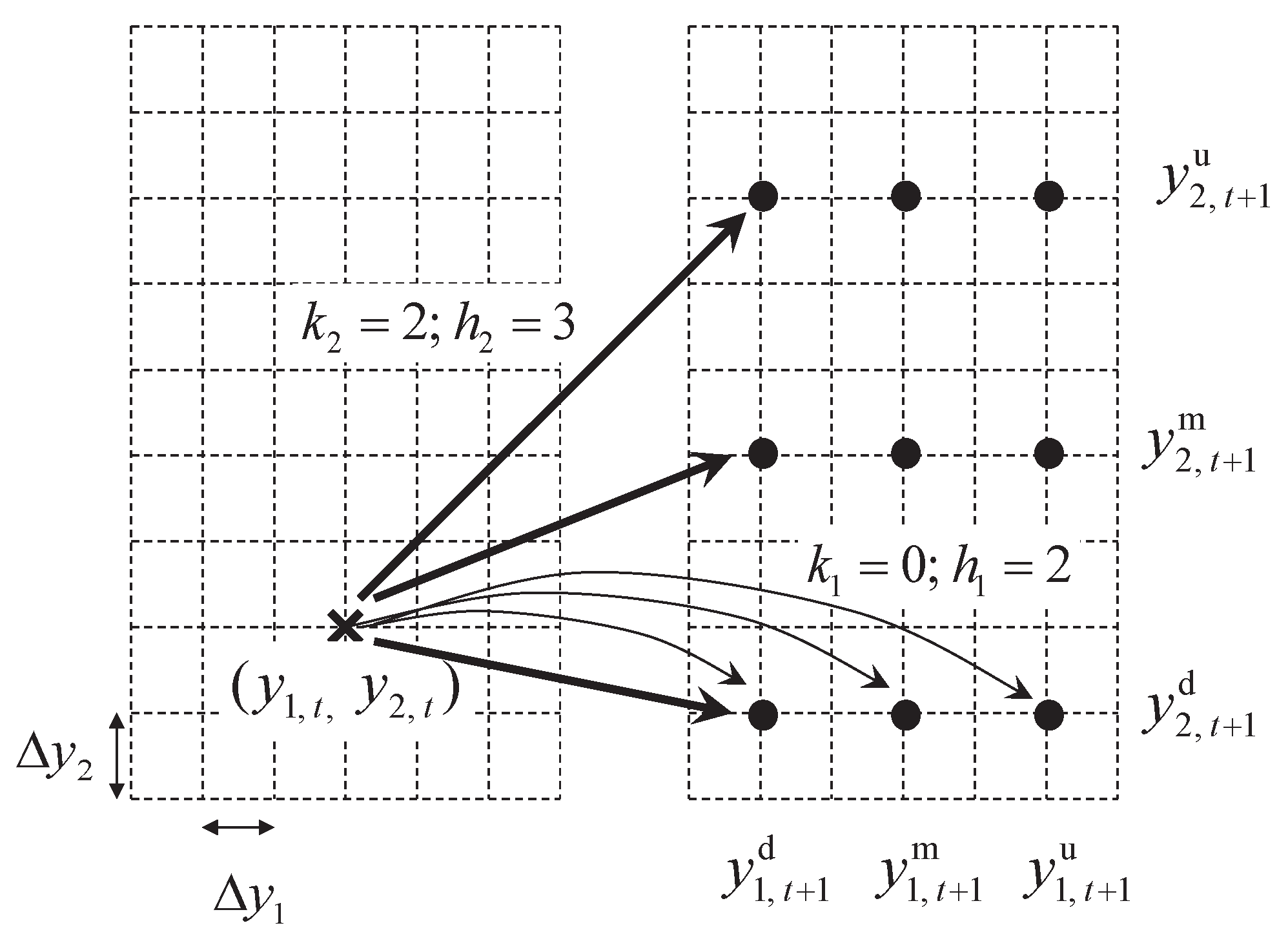
Our idea of using two-factor trinomial lattices to approximate (22a)–(22b) follows the one proposed by Hull and White (1994): obtain a one-factor trinomial lattice for each state variable first, then integrate both lattices to one such that nine branches ($3\times 3$) emanating from each lattice node. Let $\Delta y_l=c_l{\sigma }_l^s\sqrt{\Delta t}$, $l=1,2$, a definition extended directly from that in the one-factor case in Section 2. Assume the one-factor discrete price increment, branching factor for $y_l$, and branch jump size are $\Delta y_l$, $k_l$, and $h_l$, $l=1,2$, respectively, as defined in Section 2. An example is given in Figure 1, where a node $(y_{1,t},y_{2,t})$ at time t is shown in the left panel. The first one calculates $k_l$ and $h_l$ using (5) and (9), respectively, for each factor l to determine the three nodes $y_{l,t+1}^{\mathrm{u}}$, $y_{l,t+1}^{\mathrm{m}}$, and $y_{l,t+1}^{\mathrm{d}}$ at time $t+1$ that each factor l will map into. The nine nodes of their combinations at $t+1$ are shown in the right panel.

Figure 1. An example of node branching of our proposed two-factor lattice.

The main task is to solve the nine branching probabilities while matching the first two moments of each factor and their correlation. We further define $k_{l\mathrm{u}}\equiv k_l+h_l$, $k_{l\mathrm{m}}\equiv k_l$, and $k_{l\mathrm{d}}\equiv k_l-h_l$, $l=1,2$. At each node, to determine the nine branching probabilities $p_{ij},i,j\in \Omega$, where $\Omega \equiv \left\{\mathrm{u},\mathrm{m},\mathrm{d}\right\}$, one solves the following linear system, denoted by $\left(Q_0\right)$:$\left(Q_0\right)$

$$\begin{array}{ccc}\hfill \sum _{i,j\in \Omega }{p}_{ij}{k}_{1i}\Delta y_1& =\hfill & \hfill {\mu }_1\Delta t,\end{array}$$

(24a)

$$\begin{array}{ccc}\hfill \sum _{i,j\in \Omega }{p}_{ij}{k}_{2j}\Delta y_2& =\hfill & \hfill {\mu }_2\Delta t,\end{array}$$

(24b)

$$\begin{array}{ccc}\hfill \sum _{i,j\in \Omega }{p}_{ij}{k}_{1i}^2\Delta y_1^2& =\hfill & \hfill {\mu }_1^2\Delta t^2+{\sigma }_1^2\Delta t,\end{array}$$

(24c)

$$\begin{array}{ccc}\hfill \sum _{i,j\in \Omega }{p}_{ij}{k}_{2j}^2\Delta y_2^2& =\hfill & \hfill {\mu }_2^2\Delta t^2+{\sigma }_2^2\Delta t,\end{array}$$

(24d)

$$\begin{array}{ccc}\hfill \sum _{i,j\in \Omega }{p}_{ij}{k}_{1i}{k}_{2j}\Delta y_1\Delta y_2& =\hfill & \hfill \rho {\sigma }_1{\sigma }_2\Delta t+{\mu }_1{\mu }_2\Delta t^2,\end{array}$$

(24e)

$$\begin{array}{ccc}\hfill \sum _{i,j\in \Omega }{p}_{ij}& =\hfill & \hfill 1,\end{array}$$

(24f)

$$\begin{array}{ccc}\hfill p_{ij}& \ge \hfill & \hfill 0,\forall i,j\in \Omega \end{array}$$

(24g)

At each node of the trinomial lattice, it is required to solve $\left(Q_0\right)$ to determine the branching probabilities, which has nine variables, six linear equations, and nine nonnegativity inequalities. In optimization terminology, $\left(Q_0\right)$ is said to be feasible if a (feasible) solution exists that meets all constraints. Otherwise, $\left(Q_0\right)$ is said to be infeasible, which means that some probabilities must be negative or greater than 1. Lattice feasibility refers to the condition where $\left(Q_0\right)$ is feasible for all possible nodes in a lattice. In the next proposition, we will show that lattice feasibility is a necessary condition for weak convergence of the proposed two-factor lattice.

Proposition 5.

Let $(Y_{1,t}^{\Delta t},Y_{2,t}^{\Delta t})$ denote the trinomial lattice of the two-factor process $(Y_{1,t},Y_{2,t})$ defined in (22a)–(22b) with $\Delta y_l=c_l{\sigma }_l^s\sqrt{\Delta t}$, and $k_l\left(y\right)$ and $h_l\left(y\right)$ defined by (5) and (9), respectively, for $l=1,2$. Suppose that $(Y_{1,0}^{\Delta t},Y_{2,0}^{\Delta t})=(Y_{1,0},Y_{2,0})$ and the following conditions

$$\begin{array}{ccc}\hfill 0\le p_{ij}\le 1,i,j\in \Omega & & \hfill \end{array}$$

(25a)

$$\begin{array}{ccc}\hfill \mathsf{E}\left[(Y_{l,t+\Delta t}^{\Delta t}-y_l)\right|(Y_{1,t}^{\Delta t},Y_{2,t}^{\Delta t})=(y_1,y_2)]& =\hfill & \hfill {\mu }_l\Delta t,l=1,2\end{array}$$

(25b)

$$\begin{array}{ccc}\hfill \mathsf{E}\left[{(Y_{l,t+\Delta t}^{\Delta t}-y_l)}^2\right|(Y_{1,t}^{\Delta t},Y_{2,t}^{\Delta t})=(y_1,y_2)]& =\hfill & \hfill {\sigma }_l^2\Delta t+{\mu }_l^2\Delta t^2,l=1,2\end{array}$$

(25c)

$$\begin{array}{ccc}\hfill \mathsf{E}\left[(Y_{1,t+\Delta t}^{\Delta t}-y_1)(Y_{2,t+\Delta t}^{\Delta t}-y_2)\right|(Y_{1,t}^{\Delta t},Y_{2,t}^{\Delta t})=(y_1,y_2)]& =\hfill & \hfill \rho {\sigma }_1{\sigma }_2\Delta t+{\mu }_1{\mu }_2\Delta t^2\end{array}$$

(25d)

hold for all lattice node $(y_1,y_2)$ and for all time interval $\Delta t$. As $\Delta t\to 0$, $(Y_{1,t}^{\Delta t},Y_{2,t}^{\Delta t})$ converges weakly to the diffusion process $(Y_{1,t},Y_{2,t})$.

3.1. Feasibility of the General Lattice

Consider the nine branches that emanated from a fixed node, where the one-factor branching probabilities are assumed to be $\{{\tilde{p}}_{l\mathrm{u}},{\tilde{p}}_{l\mathrm{m}},{\tilde{p}}_{l\mathrm{d}}\}$, $l=1,2$. These probabilities are denoted with a tilde to indicate that they are not variables. In addition, assume at this node that the corresponding error factors of the branching and the jump sizes are ${ϵ}_l$ and ${\gamma }_l$, $l=1,2$. The branching probabilities can be obtained as follows (cf. (15a)–(15c)):

$$\begin{array}{ccc}\hfill {\tilde{p}}_{l\mathrm{u}}& =\hfill & \hfill \frac{1}{2}\left(\frac{{ϵ}_l^2}{h_l^2}+\frac{{ϵ}_l}{h_l}+\frac{{\gamma }_l^2}{c_l^2}\right)\end{array}$$

(26a)

$$\begin{array}{ccc}\hfill {\tilde{p}}_{l\mathrm{d}}& =\hfill & \hfill \frac{1}{2}\left(\frac{{ϵ}_l^2}{h_l^2}-\frac{{ϵ}_l}{h_l}+\frac{{\gamma }_l^2}{c_l^2}\right)\end{array}$$

(26b)

$$\begin{array}{ccc}\hfill {\tilde{p}}_{l\mathrm{m}}& =\hfill & \hfill 1-\left(\frac{{ϵ}_l^2}{h_l^2}+\frac{{\gamma }_l^2}{c_l^2}\right)\end{array}$$

(26c)

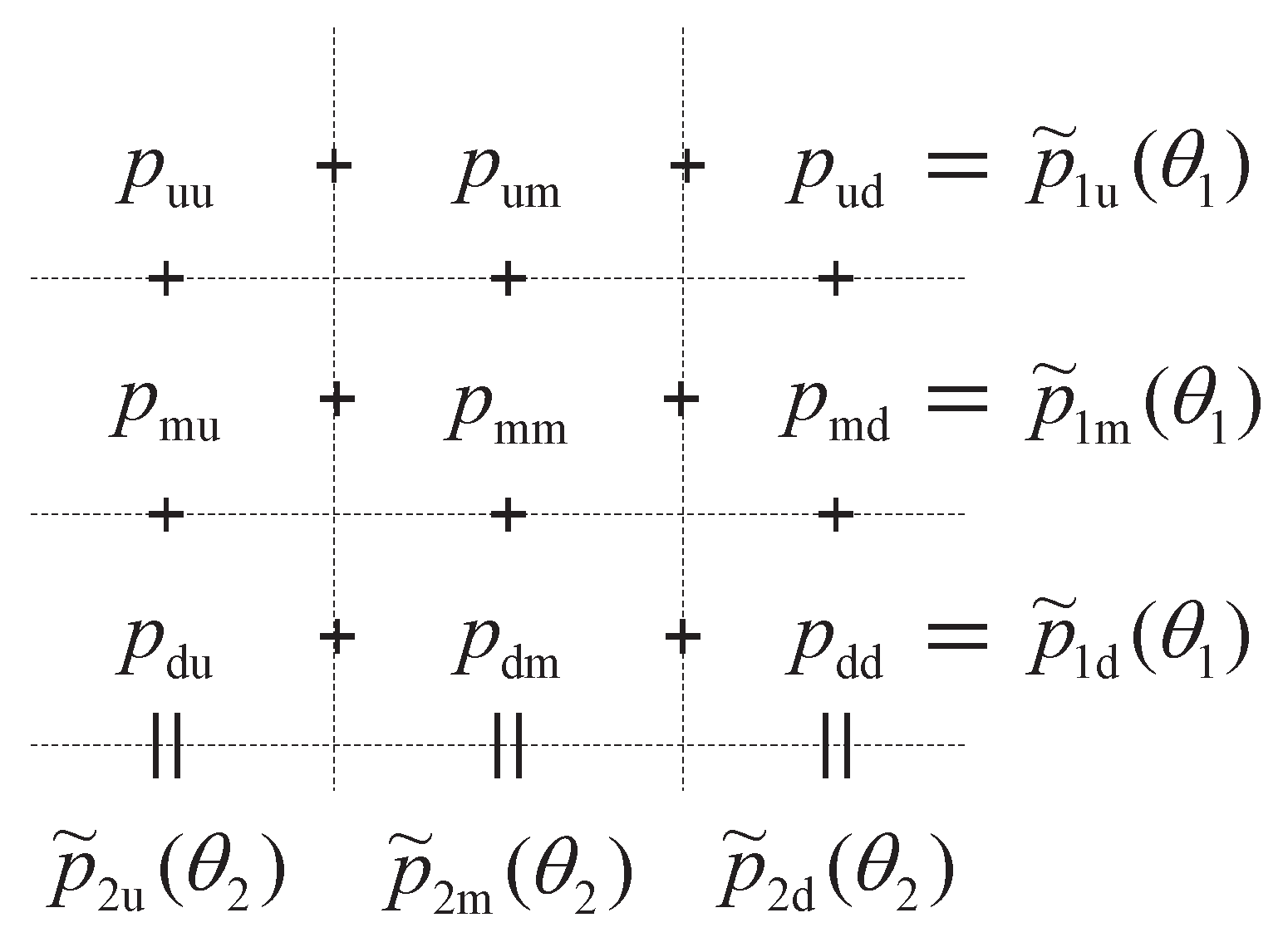
The key step is to rewrite $\left(Q_0\right)$ to the following equivalent form $\left(Q\right)$, in terms of $\left\{{\tilde{p}}_{li}\right\}$, $i\in \Omega$, and ${ϵ}_l,{\gamma }_l$, $l=1,2$: $\left(Q({ϵ}_1,x_1,{\gamma }_1,h_1,{ϵ}_2,x_2,{\gamma }_2,h_2)\right)$

$$\begin{array}{ccc}\hfill \sum _{j\in \Omega }{p}_{\mathrm{u}j}& =\hfill & \hfill {\tilde{p}}_{1\mathrm{u}}\end{array}$$

(27a)

$$\begin{array}{ccc}\hfill \sum _{j\in \Omega }{p}_{\mathrm{d}j}& =\hfill & \hfill {\tilde{p}}_{1\mathrm{d}}\end{array}$$

(27b)

$$\begin{array}{ccc}\hfill \sum _{i\in \Omega }{p}_{i\mathrm{u}}& =\hfill & \hfill {\tilde{p}}_{2\mathrm{u}}\end{array}$$

(27c)

$$\begin{array}{ccc}\hfill \sum _{i\in \Omega }{p}_{i\mathrm{d}}& =\hfill & \hfill {\tilde{p}}_{2\mathrm{d}}\end{array}$$

(27d)

$$\begin{array}{ccc}\hfill p_{\mathrm{uu}}+p_{\mathrm{dd}}-p_{\mathrm{ud}}-p_{\mathrm{du}}& =\hfill & \hfill \rho \frac{{\gamma }_1{\gamma }_2}{c_1{c}_2}+\frac{{ϵ}_1{ϵ}_2}{h_1{h}_2}\end{array}$$

(27e)

$$\begin{array}{ccc}\hfill \sum _{i,j\in \Omega }{p}_{ij}& =\hfill & \hfill 1\end{array}$$

(27f)

$$\begin{array}{ccc}\hfill p_{ij}& \ge \hfill & \hfill 0,\forall i,j\in \Omega .\end{array}$$

(27g)

To maintain legibility, we denote ${\theta }_l\equiv ({ϵ}_l,x_l,{\gamma }_l,h_l)\in {\Theta }_l\left({\underline{h}}_l\right)$, $l=1,2$, where

$${\Theta }_l\left({\underline{h}}_l\right)\equiv \left\{{\theta }_l\right|\left(7\right),\left(14\right),\left(13a\right)-\left(13b\right),\forall h_l\ge {\underline{h}}_l\},l=1,2.$$

(28)

In (28), ${\Theta }_l\left({\underline{h}}_l\right)$ covers all possible nodes in $Y_l$, $l=1,2$. $\left(Q\right)$ is denoted with $({\theta }_1,{\theta }_2)$ to emphasize that it is a ‘local’ problem associated with some specific lattice node (as ${\tilde{p}}_{l\mathrm{u}}$ and ${\tilde{p}}_{l\mathrm{d}}$ are functions of ${\theta }_l$, $l=1,2$). Equations (27a)–(27d) intend to match the means and variances of the price deviations of the two factors, which have been met by the marginal probabilities $\left\{{\tilde{p}}_{1j}\right\}$ and $\left\{{\tilde{p}}_{2j}\right\}$, $j\in \Omega$. Equation (27e) is derived from (24e) with some algebra.

Consider an initial solution $p_{ij}={\tilde{p}}_{1i}{\tilde{p}}_{2j},i,j\in \Omega$, which satisfies (27a)–(27f) but (27e), unless $\rho =0$. To determine the range of $\rho$ on the right-hand side (RHS) of (27e) that $\left(Q\right)$ is feasible, consider the following two linear programs:

$$\begin{array}{c}\hfill R^{min}({\theta }_1,{\theta }_2)\equiv \underset{p_{ij},i,j\in \Omega }{min}\{p_{\mathrm{uu}}+p_{\mathrm{dd}}-p_{\mathrm{ud}}-p_{\mathrm{du}}|\left(Q\right)\mathrm{excluding}\left(27e\right)\}\end{array}$$

(29a)

$$\begin{array}{c}\hfill R^{max}({\theta }_1,{\theta }_2)\equiv \underset{p_{ij},i,j\in \Omega }{max}\{p_{\mathrm{uu}}+p_{\mathrm{dd}}-p_{\mathrm{ud}}-p_{\mathrm{du}}|\left(Q\right)\mathrm{excluding}\left(27e\right)\}\end{array}$$

(29b)

For a given set of $({\theta }_1,{\theta }_2)$, it is clear that $\left(Q\right)$ is feasible, if, and only if, the RHS of (27e) is between $R^{min}$ and $R^{max}$, i.e.,

$$R^{min}({\theta }_1,{\theta }_2)\le \rho \frac{{\gamma }_1{\gamma }_2}{c_1{c}_2}+\frac{{ϵ}_1{ϵ}_2}{h_1{h}_2}\le R^{max}({\theta }_1,{\theta }_2).$$

(30)

Therefore, for ${\theta }_l\in {\Theta }_l\left({\underline{h}}_l\right)$, $l=1,2$, we have

$$c_1{c}_2·\underset{{\theta }_1,{\theta }_2}{max}\frac{1}{{\gamma }_1{\gamma }_2}\left(R^{min}({\theta }_1,{\theta }_2)-\frac{{ϵ}_1{ϵ}_2}{h_1{h}_2}\right)\le \rho \le c_1{c}_2·\underset{{\theta }_1,{\theta }_2}{min}\frac{1}{{\gamma }_1{\gamma }_2}\left(R^{max}({\theta }_1,{\theta }_2)-\frac{{ϵ}_1{ϵ}_2}{h_1{h}_2}\right),$$

(31)

Given the values of $c_1$ and $c_2$, using (31), the range of the correlation $\rho$ between the two factors for which the lattice can guarantee feasible branching probabilities at all nodes and all stages can be identified. Next, we will show that (31) is symmetric such that its upper bound is the negative of its lower bound.

Proposition 6.

For any arbitrary ${\theta }_l=({ϵ}_l,x_l,{\gamma }_l,h_l)\in {\Theta }_l\left({\underline{h}}_l\right)$, $l=1,2$, the following equality holds:

$$\underset{{\theta }_1,{\theta }_2}{min}\frac{1}{{\gamma }_1{\gamma }_2}\left(R^{max}({\theta }_1,{\theta }_2)-\frac{{ϵ}_1{ϵ}_2}{h_1{h}_2}\right)=-\underset{{\theta }_1,{\theta }_2}{max}\frac{1}{{\gamma }_1{\gamma }_2}\left(R^{min}({\theta }_1,{\theta }_2)-\frac{{ϵ}_1{ϵ}_2}{h_1{h}_2}\right),l=1,2.$$

(32)

Since (31) is symmetric, we can focus on solving $R^{max}$. The closed-form expression for $R^{max}$ has been derived in Tseng and Lin (2007), which is duplicated in the following proposition for the sake of clarity.

Proposition 7.

$R^{max}=min\{R_1^{max},R_2^{max},R_3^{max},R_4^{max},R_5^{max},R_6^{max}\}$, where

$$\begin{array}{ccc}\hfill R_1^{max}& =& {\tilde{p}}_{1\mathrm{u}}+{\tilde{p}}_{1\mathrm{d}}\hfill \\ \hfill R_2^{max}& =& {\tilde{p}}_{2\mathrm{u}}+{\tilde{p}}_{2\mathrm{d}}\hfill \\ \hfill R_3^{max}& =& {\tilde{p}}_{1\mathrm{u}}+{\tilde{p}}_{2\mathrm{d}}\hfill \\ \hfill R_4^{max}& =& 1-({\tilde{p}}_{1\mathrm{d}}-{\tilde{p}}_{2\mathrm{d}})-({\tilde{p}}_{2\mathrm{u}}-{\tilde{p}}_{1\mathrm{u}})\hfill \\ \hfill R_5^{max}& =& {\tilde{p}}_{2\mathrm{u}}+{\tilde{p}}_{1\mathrm{d}}\hfill \\ \hfill R_6^{max}& =& 1-({\tilde{p}}_{2\mathrm{d}}-{\tilde{p}}_{1\mathrm{d}})-({\tilde{p}}_{1\mathrm{u}}-{\tilde{p}}_{2\mathrm{u}}),\hfill \end{array}$$

where ${\tilde{p}}_{li}$, $l=1,2$, $i\in \Omega$ are from (26a)–(26c).

Note that $R_l^{max}$, $l=1,\cdots ,6$ are also functions of ${\theta }_1$ and ${\theta }_2$. It can be seen that $R_1^{max}$, $R_3^{max}$, and $R_4^{max}$ reduce to $R_2^{max}$, $R_5^{max}$, and $R_6^{max}$, and vice versa, respectively, by exchanging the factor indices 1 and 2.

Using the result from Proposition 6 to find the upper bound of (31), one needs to solve

$$\underset{{\theta }_1,{\theta }_2}{min}\underset{i=1,\cdots ,6}{min}\frac{1}{{\gamma }_1{\gamma }_2}\left\{R_i^{max}-\frac{{ϵ}_1{ϵ}_2}{h_1{h}_2}\right\}$$

(33)

for ${\theta }_l\in {\Theta }_l\left({\underline{h}}_l\right)$, $l=1,2$. It would be easier to solve if one could switch the two minimization operators in (33) as follows:

$$\underset{i=1,\cdots ,6}{min}\left\{\underset{{\theta }_1,{\theta }_2}{min}\frac{1}{{\gamma }_1{\gamma }_2}(R_i^{max}-\frac{{ϵ}_1{ϵ}_2}{h_1{h}_2})\right\}.$$

(34)

It turns out that both (33) and (34) are equivalent, which is shown in the following proposition.

Proposition 8.

Let $f_1,\cdots ,f_n:{\mathbb{R}}^n\to \mathbb{R}$ be n continuous functions and $D\subseteq {\mathbb{R}}^n$, where $n\in \mathbb{N}$ is finite. Then,

$$\underset{z\in D}{min}min\{f_1\left(z\right),\cdots ,f_n\left(z\right)\}=min\{\underset{z\in D}{min}{f}_1\left(z\right),\cdots ,\underset{z\in D}{min}{f}_n\left(z\right)\}.$$

(35)

Next, we state the main theorem of this section.

Proposition 1.

(Two-Factor Lattice Feasibility) Given a lattice configuration $(c_1,c_2,{\underline{h}}_1,{\underline{h}}_2)$, $\left(Q\right)$ is feasible for all ${\theta }_l\in {\Theta }_l\left({\underline{h}}_l\right)$, $l=1,2$, if, and only if, $\left|\rho \right|\le \overline{\rho }(c_1,c_2,{\underline{h}}_1,{\underline{h}}_2)$, where

$$\overline{\rho }(c_1,c_2,{\underline{h}}_1,{\underline{h}}_2)\equiv c_1{c}_2·min\{w_1,w_2,w_3,w_4\},$$

(36)

and

$$\begin{array}{ccc}\hfill w_1& =\hfill & \hfill \underset{{\theta }_1,{\theta }_2}{min}\frac{1}{{\gamma }_1{\gamma }_2}\left(\frac{{\varphi }_1^2}{h_1^2}-\frac{{\varphi }_1}{2h_1{h}_2}+\frac{{\gamma }_1^2}{c_1^2}\right),{\varphi }_1(h_1,h_2)\equiv min(\frac{h_1}{4h_2},\frac{1}{2}),\end{array}$$

(37a)

$$\begin{array}{ccc}\hfill w_2& =\hfill & \hfill \underset{{\theta }_1,{\theta }_2}{min}\frac{1}{{\gamma }_1{\gamma }_2}\left(\frac{{\varphi }_2^2}{h_2^2}-\frac{{\varphi }_2}{2h_1{h}_2}+\frac{{\gamma }_2^2}{c_2^2}\right),{\varphi }_2(h_1,h_2)\equiv min(\frac{h_2}{4h_1},\frac{1}{2}),\\ \hfill w_3& =\hfill & \underset{{\theta }_1,{\theta }_2}{min}\frac{1}{{\gamma }_1{\gamma }_2}\left[\frac{1}{8}({\varphi }_3^2-1)+\frac{1}{2}\left(\frac{{\gamma }_1^2}{c_1^2}+\frac{{\gamma }_2^2}{c_2^2}\right)\right],\hfill \end{array}$$

(37b)

$$\begin{array}{ccc}& & \hfill {\varphi }_3(h_1,h_2)\equiv max(1-\frac{1}{h_1}-\frac{1}{h_2},0),\end{array}$$

(37c)

$$\begin{array}{ccc}\hfill w_4& =\hfill & \hfill \underset{{\theta }_1,{\theta }_2}{min}\frac{1}{{\gamma }_1{\gamma }_2}(1-\frac{1}{2h_1})(1-\frac{1}{2h_2}).\end{array}$$

(37d)

Theorem 1 is general, but, unfortunately, no explicit functional expressions for $w_1,\cdots ,w_4$ are available because each of them requires solving a two-dimensional global minimum of a discontinuous function. However, given a set of lattice parameters $(c_1,c_2,{\underline{h}}_1,{\underline{h}}_2)$, using numerical methods, such as exhaustive search, one can easily obtain the numerical values of $w_1,\cdots ,w_4$.

From the perspective of minimizing computational requirements, one would prefer smaller values of $({\underline{h}}_1,{\underline{h}}_2)$ so that the grid size may not become too small. To achieve that, next, we try to maximize $\overline{\rho }$ over $c_1$ and $c_2$ for a given $({\underline{h}}_1,{\underline{h}}_2)$ pair:

$${\rho }_{max}({\underline{h}}_1,{\underline{h}}_2)=\underset{c_1,c_2}{max}\left\{\overline{\rho }(c_1,c_2,{\underline{h}}_1,{\underline{h}}_2)\right|c_1,c_2\text{ subject to }\left(16\right)\}.$$

(38)

Using numerical methods, Table 1 shows the values of ${\rho }_{max}$ for all 100 pairs of $({\underline{h}}_1,{\underline{h}}_2)$ for $1\le {\underline{h}}_1,{\underline{h}}_2\le 10$. Note that, since ${\rho }_{max}$ is symmetric, Table 1 only displays half of the pairs with ${\underline{h}}_1\ge {\underline{h}}_2$. From Table 1, it is clear that ${\rho }_{max}({\underline{h}}_1,{\underline{h}}_2)$ is an increasing function in ${\underline{h}}_1$ and ${\underline{h}}_2$. If one considers increasing ${\underline{h}}_1$ by 1 to be as difficult in terms of computational effort as increasing ${\underline{h}}_2$ by 1, then the diagonal elements where (${\underline{h}}_1={\underline{h}}_2$) seem to be the most efficient choices.

Table 1. The 100 values of ${\rho }_{max}({\underline{h}}_1,{\underline{h}}_2)$ for $1\le {\underline{h}}_1,{\underline{h}}_2\le 10$.

$({\underline{\mathit{h}}}_1,{\underline{\mathit{h}}}_2)$	1	2	3	4	5	6	7	8	9	10
1	0.3333	0.4957	0.5544	0.5866	0.6076	0.6222	0.6319	0.6343	0.6362	0.6376
2		0.6399	0.6892	0.7156	0.7327	0.7450	0.7539	0.7610	0.7668	0.7714
3			0.7401	0.7661	0.7834	0.7947	0.8050	0.8112	0.8170	0.8212
4				0.7949	0.8124	0.8235	0.8321	0.8393	0.8450	0.8499
5					0.8302	0.8414	0.8504	0.8571	0.8633	0.8682
6						0.8551	0.8628	0.8707	0.8751	0.8798
7							0.8735	0.8797	0.8856	0.8898
8								0.8878	0.8919	0.8961
9									0.8991	0.9033
10										0.9084

When ${\underline{h}}_1={\underline{h}}_2$, to obtain the optimal solutions $(c_1^{*},c_2^{*})$ for achieving ${\rho }_{max}$ in (38), it turns out that $w_1=w_2$ in Theorem 1 are the smallest elements in the minimum operator in (36), so a symmetrical optimal solution $c_1^{*}=c_2^{*}$ is obtained. Using numerical methods, the values of ${\rho }_{max}$ and the corresponding ($c_1^{*},c_2^{*})$ are summarized in Table 2.

Table 2. The values of ${\rho }_{max}$ and the optimal $(c_1^{*},c_2^{*})$ when ${\underline{h}}_1={\underline{h}}_2$.

${\underline{\mathit{h}}}_1={\underline{\mathit{h}}}_2$	${\mathit{\rho }}_{max}({\underline{\mathit{h}}}_1,{\underline{\mathit{h}}}_2)$	$({\mathit{c}}_1^{*},{\mathit{c}}_2^{*})$
1	0.3333	(1.7321, 1.7321)
2	0.6397	(1.3340, 1.3340)
3	0.7400	(1.2052, 1.2052)
4	0.7949	(1.1469, 1.1469)
5	0.8320	(1.1145, 1.1145)
6	0.8551	(1.0931, 1.0931)
7	0.8735	(1.0792, 1.0792)
8	0.8878	(1.0686, 1.0686)
9	0.8991	(1.0602, 1.0602)
10	0.9084	(1.0543, 1.0543)

As an example, if $\rho =-0.8$, using the optimized $(c_1^{*},c_2^{*})$ from Table 2, one can use ${\underline{h}}_1={\underline{h}}_2=5$ by using $(c_1,c_2)=(1.1145,1.1145)$ obtained from the Appendix A. Note that the results presented in this section are for general two-factor lattices. If the two underlying diffusion processes have some special structures, e.g., the class of square root volatility models, then ${\rho }_{max}$ may be further increased so that the required $({\underline{h}}_1,{\underline{h}}_2)$ that guarantees lattice feasibility may be lowered. In the next section, we focus on the Heston SV model, for which explicit functional expressions for $w_1,\cdots ,w_4$ are available.

3.2. Lattice for the Heston SV Model

Consider the Heston SV model (Heston 1993) as follows:

$$\begin{array}{ccc}\hfill d{Y}_{1,t}& =\hfill & \hfill \mu dt+\sqrt{Y_{2,t}}d{W}_{1,t}\end{array}$$

(39a)

$$\begin{array}{ccc}\hfill d{Y}_{2,t}& =\hfill & \hfill -\lambda (Y_{2,t}-m)dt+\xi \sqrt{Y_{2,t}}d{W}_{2,t},\end{array}$$

(39b)

where $Y_{1,t}=ln{S}_t$ is the logarithm of the stock price; $\mu$, $\lambda$, m, and $\xi$ are positive constants.

Since both volatilities in (39a) and (39b) are functions of $Y_2$, we focus on the MR process of $Y_2$. As mentioned in Section 2.2, if the Feller condition is satisfied, $y_2^{min}>0$ exists for (39b). Based on $y_2^{min}$, we can identify positive ${\sigma }_2^{min}$ and ${\sigma }_2^s$. Once ${\sigma }_2^s$ is obtained, we set

$${\sigma }_1^s={\sigma }_2^s/\xi .$$

(40)

Proposition 9.

To implement the Heston SV model given in (39a)–(39b) using the proposed trinomial lattice and (40), if ${\underline{h}}_1={\underline{h}}_2$, then $h_1=h_2$, $x_1=x_2$, and ${\gamma }_1={\gamma }_2$ at all nodes.

Using Proposition 9, we will show that Theorem 1 has an explicit functional form for $\overline{\rho }$ if we set ${\underline{h}}_1={\underline{h}}_2$. Since ${\mu }_1$ is a constant, ${ϵ}_1$ is a fixed constant for all nodes. We denote it as ${\widetilde{ϵ}}_1$. Without loss of generality, we assume ${\widetilde{ϵ}}_1=0$. To make ${\widetilde{ϵ}}_1=0$, from (5), we need to have

$$\frac{{\mu }_1\Delta t}{c_1{\sigma }_1^s\sqrt{\Delta t}}=\frac{{\mu }_1\sqrt{\Delta t}}{c_1{\sigma }_1^s}=\mathrm{the\; nearest\; integer}=k_1.$$

(41)

This can be achieved by adjusting the value of $c_1$, ${\sigma }_1^{min}$, or $\Delta t$. Adjusting $c_1$ and/or $\Delta t$ is more straightforward than adjusting ${\sigma }_1^{min}$. However, since $c_1$ is a parameter for lattice configuration, we recommend adjusting the value of $\Delta t$ slightly to eliminate the remainder of (41) in order to make ${\widetilde{ϵ}}_1=0$.

With ${ϵ}_1=0$ and ${\underline{h}}_1={\underline{h}}_2=\underline{h}$, using (31), the condition for lattice feasibility can be significantly simplified as follows:

$$\underset{{\theta }_1,{\theta }_2}{max}\frac{1}{{\gamma }^2}\left(R^{min}({\theta }_1,{\theta }_2)\right)\le \frac{\rho }{c_1{c}_2}\le \underset{{\theta }_1,{\theta }_2}{min}\frac{1}{{\gamma }^2}\left(R^{max}({\theta }_1,{\theta }_2)\right),$$

(42)

for ${\theta }_l\in {\Theta }_l\left(\underline{h}\right)$, $l=1,2$.

Theorem 2.

(Lattice feasibility for the Heston SV) Pertaining to the Heston SV model in (39a)–(39b), assume ${\underline{h}}_1={\underline{h}}_2=\underline{h}$ and ${ϵ}_1=0$. Given a lattice configuration $(c_1,c_2,\underline{h})$, $\left(Q\right)$ is feasible for all ${\theta }_l\in {\Theta }_l\left(\underline{h}\right)$, $l=1,2$, if, and only if, $\rho \le {\overline{\rho }}^{\mathit{H}}(c_1,c_2,\underline{h})$, where

$${\overline{\rho }}^{\mathit{H}}(c_1,c_2,\underline{h})=c_1{c}_2·min\{w_1^{\mathit{H}},w_2^{\mathit{H}},w_3^{\mathit{H}},w_4^{\mathit{H}}\},$$

(43)

where

$$\begin{array}{ccc}\hfill w_1^{\mathit{H}}& =\hfill & \hfill \frac{1}{c_1^2}\end{array}$$

(44a)

$$\begin{array}{ccc}\hfill w_2^{\mathit{H}}& =\hfill & \hfill \frac{1}{c_2^2}\end{array}$$

(44b)

$$\begin{array}{ccc}\hfill w_3^{\mathit{H}}& =\hfill & \hfill \frac{1}{2}(\frac{1}{c_1^2}+\frac{1}{c_2^2})-\frac{1}{4(max(\underline{h},2)-0.5)},\end{array}$$

(44c)

$$\begin{array}{ccc}\hfill w_4^{\mathit{H}}& =\hfill & \hfill \frac{\underline{h}(\underline{h}-0.5)}{{(\underline{h}+0.5)}^2}\end{array}$$

(44d)

Next, we try to maximize ${\overline{\rho }}^{\mathit{H}}$ by adjusting the lattice configuration $(c_1,c_2)$ while maintaining lattice feasibility. Let

$${\rho }_{max}^{\mathit{H}}\left(\underline{h}\right)=\underset{c_1,c_2}{max}\left\{{\overline{\rho }}^{\mathit{H}}(c_1,c_2,\underline{h})\right|c_1,c_2\text{ subject to }\left(16\right)\}.$$

(45)

Using numerical methods, the solution of (45) is obtained as follows. When $\underline{h}\le 2$, ${\rho }_{max}^{\mathit{H}}$ is achieved at the lower bounds of $c_1$ and $c_2$, where $c_1=c_2=\sqrt{(\underline{h}+0.5)/(\underline{h}-0.5)}$, and ${\rho }_{max}^{\mathit{H}}$ is determined by $w_3^{\mathit{H}}$. When $\underline{h}\ge 3$, ${\rho }_{max}^{\mathit{H}}$ is achieved at $c_1=\sqrt{(\underline{h}+0.5)/(\underline{h}-0.5)}$, the lower bound, and $c_2$ at the point where $w_3^{\mathit{H}}=w_4^{\mathit{H}}$. That is,

$${\rho }_{max}^{\mathit{H}}\left(\underline{h}\right)=c_1^{\mathit{H}}\left(\underline{h}\right)c_2^{\mathit{H}}\left(\underline{h}\right)\frac{\underline{h}(\underline{h}-0.5)}{{(\underline{h}+0.5)}^2},\underline{h}\ge 3,$$

(46)

where

$$\begin{array}{ccc}\hfill c_1^{\mathit{H}}\left(\underline{h}\right)& =& \sqrt{\frac{\underline{h}+0.5}{\underline{h}-0.5}}\hfill \end{array}$$

(47)

$$\begin{array}{ccc}\hfill c_2^{\mathit{H}}\left(\underline{h}\right)& =& \sqrt{\frac{{(\underline{h}+0.5)}^2(\underline{h}-0.5)}{{\underline{h}}^3-{\underline{h}}^2+1.25\underline{h}}}.\hfill \end{array}$$

(48)

It can be seen that ${\rho }_{max}^{\mathit{H}}\left(\underline{h}\right)$ approaches 1 as $\underline{h}$ increases. The value of ${\rho }_{max}^{\mathit{H}}\left(\underline{h}\right)$ for $\underline{h}=1,\cdots ,10$ is given in Table 3, along with the corresponding $(c_1^{\mathit{H}},c_2^{\mathit{H}})$. Note that ${\rho }_{max}^{\mathit{H}}\left(\underline{h}\right)$ is symmetric in $c_1$ and $c_2$. Therefore, another solution for ${\rho }_{max}^{\mathit{H}}\left(\underline{h}\right)$ is to switch $c_1^{\mathit{H}}$ and $c_2^{\mathit{H}}$.

Table 3. The values of ${\rho }_{max}^{\mathit{H}}$ (with ${\widetilde{ϵ}}_1=0$).

$\underline{\mathit{h}}$	${\mathit{\rho }}_{max}^{\mathit{H}}\left(\underline{\mathit{h}}\right)$	$({\mathit{c}}_1^{\mathit{H}},{\mathit{c}}_2^{\mathit{H}})$	$\underline{\mathit{h}}$	${\mathit{\rho }}_{max}^{\mathit{H}}\left(\underline{\mathit{h}}\right)$	$({\mathit{c}}_1^{\mathit{H}},{\mathit{c}}_2^{\mathit{H}})$
1	0.5000	(1.7321, 1.7321)	6	0.9453	(1.0871, 1.1133)
2	0.7222	(1.2910, 1.2910)	7	0.9549	(1.0742, 1.0989)
3	0.8596	(1.1832, 1.1866)	8	0.9616	(1.0646, 1.0877)
4	0.9065	(1.1339, 1.1564)	9	0.9667	(1.0572, 1.0787)
5	0.9308	(1.1055, 1.1319)	10	0.9705	(1.0513, 1.0714)

Back to the previous example, if $\rho =-0.8$, now it only requires ${\underline{h}}_1={\underline{h}}_2=3$ with $(c_1,c_2)=$ (1.1832,1.1866) or (1.1866, 1.1832) to achieve lattice feasibility, a reduction from ${\underline{h}}_1={\underline{h}}_2=5$ of the optimized general model.

4. Impact of Lattice Infeasibility on Option Valuation

In this section, we investigate how much lattice infeasibility could impact option valuation. Consider the following SV model of Heston (1993) where the stock price ($S_t$) and the instantaneous variance ($V_t$) under the risk neutral measure are defined as follows:

$$\begin{array}{ccc}\hfill dln{S}_t& =\hfill & \hfill (r-q-\frac{V_t}{2})dt+\sqrt{V_t}d{W}_{1,t},\end{array}$$

(49a)

$$\begin{array}{ccc}\hfill d{V}_t& =\hfill & \hfill \lambda (m-V_t)dt+\xi \sqrt{V_t}d{W}_{2,t},\end{array}$$

(49b)

where r is the constant risk-free rate, q is the dividend yield, and $d{W}_{1,t}$ and $d{W}_{2,t}$ are Wiener processes such that $d{W}_{1,t}·d{W}_{2.t}=\rho dt$.

4.1. An Optimization Perspective

The problem $\left(Q\right)$ contains six linear equations with nine variables and a nonnegativity constraint. Since $\left(Q\right)$ has no linear independence of the linear equations, these linear equations have infinitely many solutions (sets of branching probabilities). Therefore, the key is the nonnegativity constraint, which requires a solution to be a set of legitimate probabilities. When the term ‘lattice feasibility’ was coined by Tseng and Lin (2007), there was an implication of using optimization to determine branching probabilities. The idea was to add an objective function to be optimized subject to $\left(Q\right)$. Since not all feasible solutions contribute the same to the objective function, using optimization would find not only a feasible solution, but an optimal solution. The objective function in this context refers to the quality of fitting the probability distribution of the underlying uncertainties. The authors in Tseng and Lin (2007) used the following objective function:

$$\underset{p_{ij}}{min}\sum _{i,j\in \Omega }{(p_{ij}-{\tilde{p}}_{1i}{\tilde{p}}_{2j})}^2,$$

(50)

where $p_{ij}$, $i,j\in \Omega$ are subject to $\left(Q\right)$; and ${\tilde{p}}_{1i}$ and ${\tilde{p}}_{2j}$ are marginal probabilities obtained from (26a)–(26c). Tseng and Lin (2007) showed that doing so best fits the probability distribution of the underlying variables in some measure.

The optimization problem in (50) is a standard quadratic programming (QP) problem with linear constraints. Apparently, the optimal solution of (50) is $p_{ij}={\tilde{p}}_{1i}{\tilde{p}}_{2j}$, $i,j\in \Omega$ when $\rho =0$. When $\rho \ne 0$, this optimization problem finds the solution that has the least deviation from the solution of the uncorrelated case. At each node, their approach requires solving a simple optimization problem to determine branching probabilities for $\left(Q\right)$. We adopt this approach in this paper and refer to it as Best-Fit. Although solving a (QP) at each node may seem cumbersome, we have developed an iterative method to identify the binding constraints at optimality. Once the binding constraints are identified, the corresponding feasible solution is the optimal one due to the convexity of the QP. This approach is very efficient as it usually takes a few trials to correctly identify the binding constraints.

On the other hand, we need a counterpart method for determining branching probabilities that works well in practice but may not guarantee lattice feasibility. We consider the popular lattice approach proposed by Hull and White (1994) (denoted by H&W) as this counterpart method. Note that the comparison is conducted in the same lattice framework such that the lattice structure is exactly the same except for their respective methods of determining branching probabilities at each node: the first is by Best-Fit and the second by H&W.

When $\rho <0$, Hull and White (1994) suggests with $\delta =\rho /36$:

$$\begin{array}{c}\hfill \left[\begin{array}{ccc}\hfill p_{\mathrm{du}}& \hfill p_{\mathrm{mu}}& \hfill p_{\mathrm{uu}}\\ \hfill p_{\mathrm{dm}}& \hfill p_{\mathrm{mm}}& \hfill p_{\mathrm{um}}\\ \hfill p_{\mathrm{dd}}& \hfill p_{\mathrm{md}}& \hfill p_{\mathrm{ud}}\end{array}\right]=\left[\begin{array}{ccc}\hfill {\tilde{p}}_{1\mathrm{d}}{\tilde{p}}_{2\mathrm{u}}& \hfill {\tilde{p}}_{1\mathrm{m}}{\tilde{p}}_{2\mathrm{u}}& \hfill {\tilde{p}}_{1\mathrm{u}}{\tilde{p}}_{2\mathrm{u}}\\ \hfill {\tilde{p}}_{1\mathrm{d}}{\tilde{p}}_{2\mathrm{m}}& \hfill {\tilde{p}}_{1\mathrm{m}}{\tilde{p}}_{2\mathrm{m}}& \hfill {\tilde{p}}_{1\mathrm{u}}{\tilde{p}}_{2\mathrm{m}}\\ \hfill {\tilde{p}}_{1\mathrm{d}}{\tilde{p}}_{2\mathrm{d}}& \hfill {\tilde{p}}_{1\mathrm{m}}{\tilde{p}}_{2\mathrm{d}}& \hfill {\tilde{p}}_{1\mathrm{u}}{\tilde{p}}_{2\mathrm{d}}\end{array}\right]+\left[\begin{array}{ccc}\hfill -\delta & \hfill -4\delta & \hfill +5\delta \\ \hfill -4\delta & \hfill +8\delta & \hfill -4\delta \\ \hfill +5\delta & \hfill -4\delta & \hfill -\delta \end{array}\right];\end{array}$$

(51a)

and similarly when $\rho <0$,

$$\begin{array}{c}\hfill \left[\begin{array}{ccc}\hfill p_{\mathrm{du}}& \hfill p_{\mathrm{mu}}& \hfill p_{\mathrm{uu}}\\ \hfill p_{\mathrm{dm}}& \hfill p_{\mathrm{mm}}& \hfill p_{\mathrm{um}}\\ \hfill p_{\mathrm{dd}}& \hfill p_{\mathrm{md}}& \hfill p_{\mathrm{ud}}\end{array}\right]=\left[\begin{array}{ccc}\hfill {\tilde{p}}_{1\mathrm{d}}{\tilde{p}}_{2\mathrm{u}}& \hfill {\tilde{p}}_{1\mathrm{m}}{\tilde{p}}_{2\mathrm{u}}& \hfill {\tilde{p}}_{1\mathrm{u}}{\tilde{p}}_{2\mathrm{u}}\\ \hfill {\tilde{p}}_{1\mathrm{d}}{\tilde{p}}_{2\mathrm{m}}& \hfill {\tilde{p}}_{1\mathrm{m}}{\tilde{p}}_{2\mathrm{m}}& \hfill {\tilde{p}}_{1\mathrm{u}}{\tilde{p}}_{2\mathrm{m}}\\ \hfill {\tilde{p}}_{1\mathrm{d}}{\tilde{p}}_{2\mathrm{d}}& \hfill {\tilde{p}}_{1\mathrm{m}}{\tilde{p}}_{2\mathrm{d}}& \hfill {\tilde{p}}_{1\mathrm{u}}{\tilde{p}}_{2\mathrm{d}}\end{array}\right]+\left[\begin{array}{ccc}\hfill +5\delta & \hfill -4\delta & \hfill -\delta \\ \hfill -4\delta & \hfill +8\delta & \hfill -4\delta \\ \hfill -\delta & \hfill -4\delta & \hfill +5\delta \end{array}\right].\end{array}$$

(51b)

4.2. Numerical Comparisons: Best-Fit vs. H&W

It is well known that the feasibility of $\left(Q\right)$ becomes harder to meet when the value of the instantaneous correlation $\rho$ is high. If one allows some branching probabilities to be negative, the corresponding probability distribution(s) of the price and/or the volatility is distorted. Depending on the degree of the distortion, there may be some impact on the option valuation. We use both approaches (Best-Fit and H&W) to value a European call option under the Heston SV model. The parameters are taken from Table 1 of Ball and Roma (1994) with $r=q=0$, $\lambda =8$, $m=V_0=0.1225,$ and $\xi =0.8$.

With $S_0=\$100$, three cases, corresponding to three different strike prices, $K=$ $80, $100, and $120, are tested with the correlation $\rho$ ranging between −0.8 and 0.8. The result is summarized in Table 4. For the lattice, we consider $n=100$ (with T = 6 months) to make sure that both methods (Best-Fit and H&W) can best fit the probability distribution of the underlying variables.

Table 4. Impact of lattice infeasibility on options pricing.

	In-the-Money (ITM)			At-the-Money (ATM)			Out-of-the-Money (OTM)			Infeasibility (%)
$\mathit{\rho }$	Exact	Best-Fit	H&W	Exact	Best-Fit	H&W	Exact	Best-Fit	H&W	Best-Fit	H&W
0.8	21.5729	21.5704	21.9341	9.8203	9.8259	9.7892	4.3276	4.3337	3.9417	0	99.79
0.7	21.6637	21.6620	21.9489	9.8140	9.8194	9.7859	4.2401	4.2454	3.9227	0	1.03
0.6	21.7499	21.7490	21.9495	9.8060	9.8107	9.7854	4.1509	4.1553	3.9221	0	0.21
0.5	21.8320	21.8313	21.9926	9.7965	9.8010	9.7776	4.0600	4.0640	3.8665	0	0.21
0.4	21.9104	21.9100	22.0347	9.7853	9.7903	9.7694	3.9672	3.9710	3.8103	0	0.11
0.3	21.9854	21.9853	22.0757	9.7726	9.7779	9.7606	3.8725	3.8760	3.7534	0	0.00
0.2	22.0571	22.0575	22.1158	9.7584	9.7640	9.7514	3.7757	3.7790	3.6958	0	0.00
0.1	22.1260	22.1267	22.1549	9.7428	9.7485	9.7417	3.6769	3.6798	3.6375	0	0.00
0.0	22.1920	22.1931	22.1931	9.7256	9.7315	9.7315	3.5759	3.5784	3.5784	0	0.00
−0.1	22.2555	22.2569	22.2304	9.7070	9.7129	9.7210	3.4726	3.4747	3.5186	0	0.00
−0.2	22.3165	22.3183	22.2669	9.6870	9.6928	9.7101	3.3668	3.3684	3.4579	0	0.00
−0.3	22.3752	22.3773	22.3026	9.6655	9.6712	9.6987	3.2584	3.2596	3.3964	0	0.00
−0.4	22.4317	22.4341	22.3375	9.6425	9.6481	9.6869	3.1472	3.1480	3.3339	0	0.11
−0.5	22.4861	22.4888	22.3717	9.6181	9.6234	9.6745	3.0330	3.0334	3.2706	0	0.21
−0.6	22.5386	22.5414	22.4051	9.5922	9.5969	9.6617	2.9157	2.9156	3.2063	0	0.21
−0.7	22.5891	22.5925	22.4052	9.5647	9.5700	9.6619	2.7949	2.7940	3.2057	0	1.03
−0.8	22.6379	22.6415	22.4165	9.5357	9.5410	9.6579	2.6703	2.6687	3.1832	0	99.79

The last two columns of Table 4 show the percentage of lattice nodes (from $t=0$ to T) that each has at least one outgoing branch with a probability either negative or exceeding unity. Note that this should not be confused with the situation where a price node at some stage has a negative probability to prevail. A lattice node may receive many incoming branches from other nodes in the previous stage. While some of the incoming branches may have negative probabilities, it is unlikely that the resultant probability for reaching this node is negative.

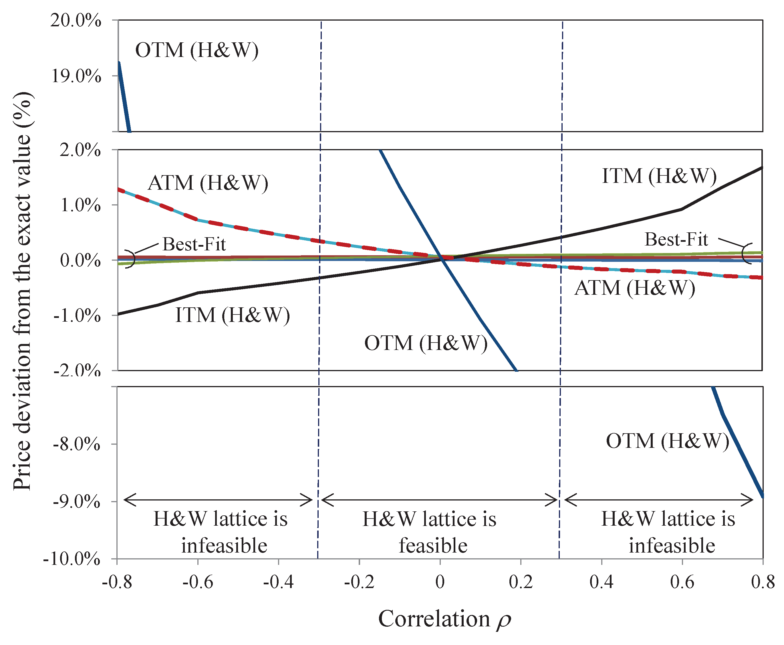
Basically, the option prices using Best-Fit are very close to the exact values, within one cent. It can be seen that Best-Fit maintains lattice feasibility for all $\rho$ values tested, while H&W meets the feasibility condition only when $\left|\rho \right|\le 0.3$. When $0.3<\left|\rho \right|\le 0.7$, there is only a very small number of nodes containing branches with negative probabilities. However, when $\left|\rho \right|=0.8$, almost all the nodes (99.79%) violate the feasibility condition. This justifies our selection of H&W as the counterpart, as this method indeed provides very good approximations of branching probabilities that solve $\left(Q\right)$. Figure 2 displays the percentage deviation of the obtained option prices from the exact ones by changing $\rho$ using Best-Fit and H&W.

Figure 2. Deviation (%) of the values of European call options from the exact ones using Best-Fit and H&W for branching probabilities.

It can be seen from Figure 2 that H&W obtains a precise value only when there is no correlation. As $\left|\rho \right|$ increases, the option value obtained by H&W starts to deviate from the exact values. The deviation is roughly a piecewise linear function of $\rho$, whose slope doubles when $\left|\rho \right|>0.6$. On the other hand, the deviations of Best-Fit are largely confined within 0.6 cents (less than 0.1%). Comparing both methods, we make the following three observations for H&W’s method:

• Consider the OTM option and the ITM option when $\left|\rho \right|\le 0.3$. Though lattice feasibility is fully maintained, the error persists for $\rho \ne 0$. Therefore, lattice feasibility alone cannot guarantee good valuation, especially with a finite time step $\Delta t$. The valuation error would converge to zero only when $\Delta t$ is sufficiently small. Therefore, lattice feasibility is merely a necessary condition for accurate valuations. From this perspective, the optimization approach for finding a feasible and optimal set of branching probabilities makes sense.
• Consider the ATM option. Its pricing errors are relatively small for all $\rho$ values tested. Even when $\rho =\left|0.8\right|$, where infeasibility occurs at almost all nodes, the error does not seem too bad (0.3% when $\rho =0.8$; 1.3% when $\rho =-0.8$). This shows that sometimes negative probabilities seem to matter less.
• Lattice infeasibility means that there are some distortions on the probability distribution of the underlying uncertainties. The effect can be overvaluation (e.g., OTM and ATM options when $\rho <0$) or undervaluation (e.g., ITM option when $\rho <0$) of the options.

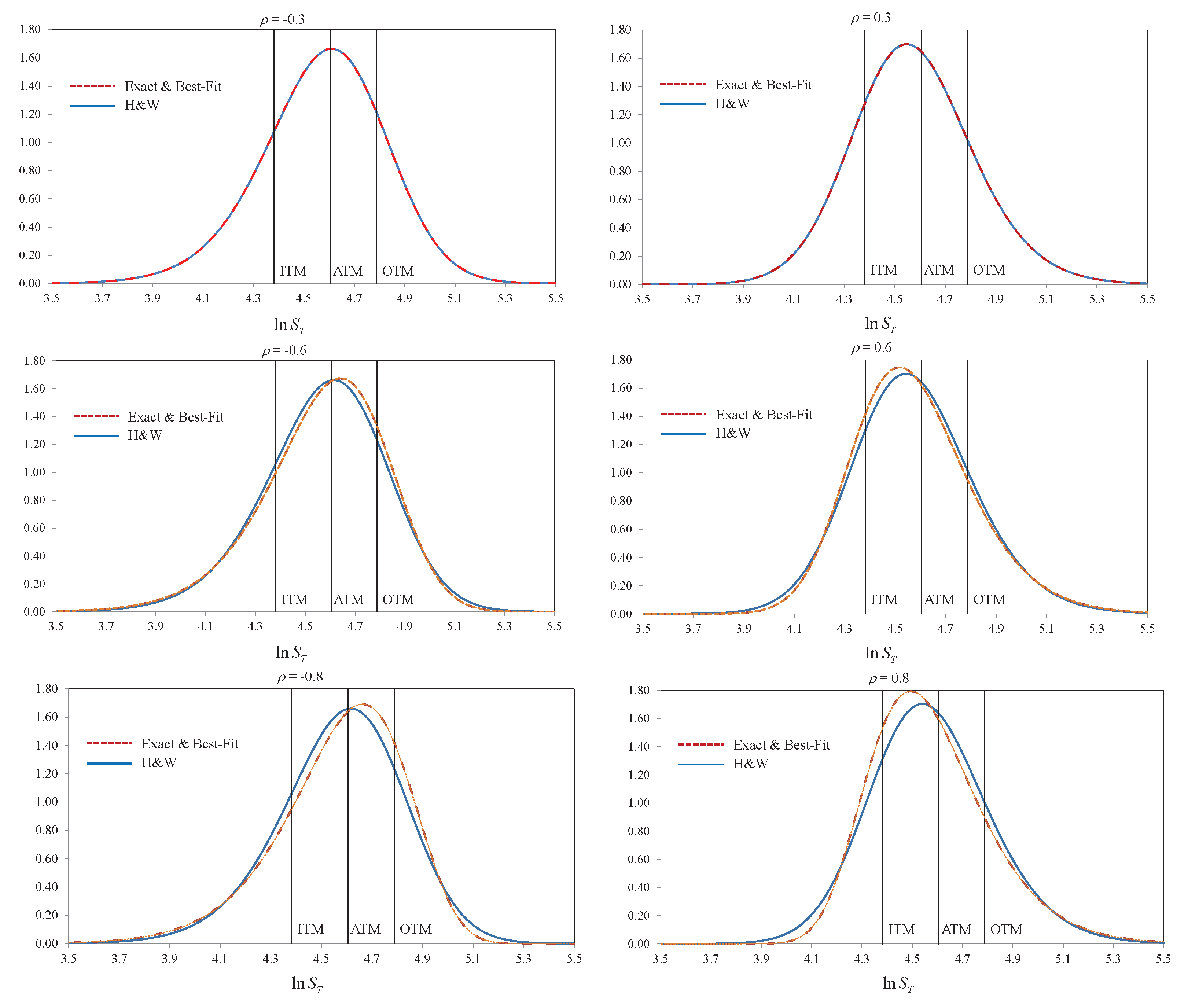
In Figure 3, we plot the exact probability density functions (PDF) of the (logarithm of the) stock price (dotted curve) at different correlation levels, and the PDF approximated by the lattice using H&W (solid curve) and Best-Fit for branching probabilities. The exact PDF is obtained from a standard integration scheme of characteristic functions (e.g., see Rough 2013). The probability distributions are taken when $\rho =\pm 0.3$, $\pm 0.6$, and $\pm 0.8$. At $\rho =\pm 0.3$, both Best-Fit and H&W achieve lattice feasibility (with the first two moments of price and volatility deviations matched). There is no visible distortion in the PDF from Figure 3, yet its OTM option price still has an error of more than 3% (12 cents). This indicates that the optimization of (50) subtly improves the approximation of the tail distribution.

Figure 3. Illustration of the underlying distributions of $ln{S}_T$.

When $\left|\rho \right|>0.3$, the discrepancy between the exact PDF and the PDF approximated by H&W becomes visible. Using $\rho =\pm 0.8$ in Figure 3 as an example, where the discrepancy is most distinct, the exact PDF and the one approximated by Best-Fit are still visually indistinguishable. In general, when $\rho >0.3$ (or $\rho <-0.3$), it can be seen that, using H&W, the price distribution is distorted such that it is slightly less skewed to the right (or left) with a bigger (or smaller) mode. In Figure 3, the three strike prices tested corresponding to OTM, ATM, and ITM options are also identified. When $\rho >0.3$ (or $\rho <-0.3$), it can be seen that using this distorted price distribution to value a European call option undervalues (or overvalues) the OTM and ATM ones, but overvalues (or undervalues) the ITM option. We make the following three additional observations:

• The price of an OTM option is directly impacted by lattice infeasibility as its value is determined by the tail distribution, which is the part of the probability distribution that is most affected by negative probabilities.
• For an ITM option, a wider part of the probability distribution becomes relevant, which tends to involve both tails and the central part, making the overall effects hard to predict.
• For an ATM option, the distorted tail part seems less important because the less distorted central part dominates the valuation.

To sum up, since, in reality, how the underlying distribution is distorted by lattice infeasibility is unknown a priori, it seems unlikely that one could exploit negative probabilities. However, if one really hopes for negative probabilities to work to their advantage, it is less likely to happen on OTM options, but more probable on ATM options.

5. Performance of the Best-Fit Lattice

In this section, we provide more numerical results for a lattice equipped with lattice feasibility and the Best-Fit method for branching probabilities. We continue to focus on the Heston SV model in (49a)–(49b). Since this approach guarantees feasible branching probabilities that also fit the underlying probability distribution well, with no surprise, all results indicate that such an approach is very reliable for accurate option valuations.

5.1. European Options Valuation

To make a comprehensive analysis of pricing errors, we compare the option prices obtained by the proposed lattice model with the exact solutions of European call options of various specifications. These specifications are drawn from combinations of the following factors: $S_0=100$, $q=2\%$ (dividend yield), $T=0.5$ years (time to maturity), $m=0.04$, $\lambda \in \{2,4,8\}$, $\xi \in \{0.3,0.6,0.9\}$, $K\in \{90,100,110\}$ (strike price), $r\in \{3\%,5\%,7\%\}$, $V_0\in \{0.02,0.04,0.08\}$, and $\rho \in \{-0.5,-0.25,0,0.25,0.5\}$. Those combinations that do not meet the Feller condition (i.e., $2\lambda m\ge {\xi }^2$) are excluded. After that, 540 sets remain for the testing. The accuracy measure used in this paper is the root mean squared error (RMSE), defined as follows:

$$\mathrm{RMSE}=\sqrt{\frac{1}{540}\sum _{i=1}^{540}{e}_i^2},$$

(52)

where the error $e_i$ is the difference between the exact value of the i-th European call option and the estimated option value using the proposed lattice model.

From Table 5, it can be seen that the pricing errors of the proposed lattice model are generally small compared with the exact option prices even if the number of time steps $\left(N\right)$ is small. For instance, when $N=10$, the RMSE of the proposed trinomial method for pricing European call options is $0.0061, which is far smaller than the bid-ask spreads observed in the market. Moreover, Table 5 indicates that the rate of convergence of the proposed method is of order $O(1/N)$.

Table 5. The accuracy of the proposed Best-Fit model for pricing European call options under the Heston SV model.

No. of Time Steps $\left(\mathit{N}\right)$	10	20	30	40
RMSE	0.0061	0.0027	0.0024	0.0013

5.2. Convergence and Complexity

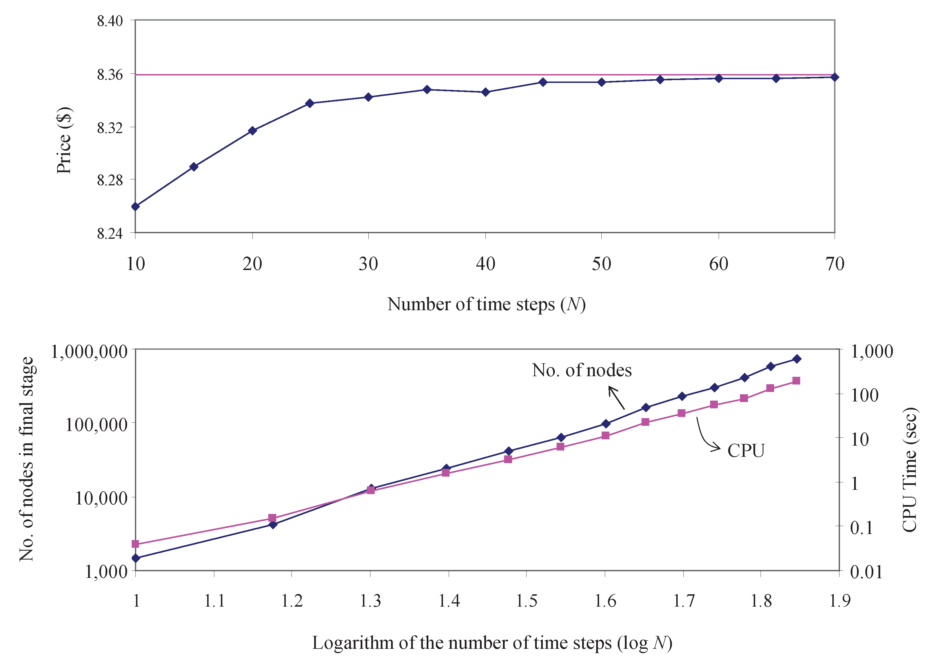
Consider another test case taken from Table 1 of Ball and Roma (1994) with $r=q=0$, $\rho =0$, $\lambda =4$, $m=V_0=0.09,$ and $\xi =0.4$. In addition, assume $T=0.5$ months, $S_0=K=\$100$. Using this example, we also investigate the convergence pattern of the option prices obtained by the proposed lattice approach and the exact value ($8.3595) when the number of time steps increases, along with its computational requirement. The results are presented in Figure 4. As seen in the upper portion of Figure 4, the option prices obtained by the proposed lattice model do converge to the exact price. We have investigated the convergence pattern for more than twenty cases, and the results are similar to those shown in Figure 4. In the lower portion, we show the CPU times required for obtaining the option values. The CPU times (in seconds) are measured on a personal computer with Intel Core 2 Duo processor E8400 of 3 GHz. We also record the number of lattice nodes in the final stage. Both the CPU times and the node numbers are displayed in logarithmic scales on both the horizontal and vertical axes. The purpose is to check whether the computational complexity is exponential. A linear behavior in a log-log graph, such as the lower portion of Figure 4, indicates that the complexity is polynomial. It is estimated for this particular instance that the CPU time is approximately of order $O\left(N^4\right)$ and the number of nodes in the final stage is of order $O\left(N^3\right)$, where N is the number of steps. The result indicates that, as N increases, most branches do recombine, which prevents the number of lattice nodes from growing exponentially with N. In this example, when $N=30$, the option value is already within 0.2% of the exact value using about three seconds of CPU time and about 40,000 nodes in the final stage. When $N=45$, the pricing error of the proposed approach is within 0.1%, using about 21 s of CPU time and 160,000 lattice nodes in the final stage. The number of lattice nodes involved in the proposed approach is indeed much greater than that of using traditional recombining lattices. However, the computation using the proposed lattice model can be managed to be quite efficient.

Figure 4. Convergence pattern of the option prices and the computational requirement.

5.3. American Options Valuation

One unique benefit for the lattice approach is its ability to value American options. We use the proposed lattice model (Best-Fit) to value American put option under the Heston SV model with parameters: strike $K=$ $100. $\lambda =3.0$, $m=0.04$, $r=0.05$, $q=0$, and $\xi =0.1$. The results are summarized in Table 6. We compare the result with that reported in Beliaeva and Nawalkha (2010), denoted by ‘B&N Tree’ in the same table. We also apply the control variate (CV) technique to value the American put as follows:

American Put (CV) = American Put (Best-Fit) +         

(European Put (Closed-Form) - European Put (Best-Fit))

Table 6. American put price computed using Best-Fit model and control variate (CV) technique, compared with the result reported in Beliaeva and Nawalkha (2010).

${\mathit{S}}_0$	$\mathit{\rho }$	${\mathit{V}}_0$	T	Best-Fit	Best-Fit CV	B&N Tree	B&N Tree CV	Euro Put	Error	Error
				$(\mathit{N}=50)$	$(\mathit{N}=50)$	$(\mathit{N}=50)$	$(\mathit{N}=50)$	True Value	(Best-Fit)	(B&N Tree)
90	−0.1	0.04	0.0833	10.0000	9.9996	10.0000	10.0001	9.6699	0.0004	0.0001
90	−0.7	0.04	0.0833	10.0000	10.0010	10.0000	9.9996	9.6533	0.0010	0.0004
100	−0.1	0.04	0.0833	2.1253	2.1262	2.1257	2.1249	2.0950	0.0009	0.0008
100	−0.7	0.04	0.0833	2.1279	2.1274	2.1250	2.1263	2.0971	0.0006	0.0013
110	−0.1	0.04	0.0833	0.1092	0.1090	0.1087	0.1090	0.1083	0.0002	0.0003
110	−0.7	0.04	0.0833	0.1259	0.1275	0.1282	0.1273	0.1265	0.0016	0.0009
90	−0.1	0.16	0.0833	10.7103	10.7109	10.7195	10.7099	10.5957	0.0006	0.0096
90	−0.7	0.16	0.0833	10.6858	10.6829	10.6709	10.6800	10.5668	0.0030	0.0091
100	−0.1	0.16	0.0833	4.2187	4.2166	4.2275	4.2163	4.1859	0.0021	0.0112
100	−0.7	0.16	0.0833	4.2196	4.2156	4.2184	4.2147	4.1852	0.0040	0.0037
110	−0.1	0.16	0.0833	1.1721	1.1667	1.1667	1.1669	1.1608	0.0053	0.0002
110	−0.7	0.16	0.0833	1.1962	1.1944	1.2176	1.1942	1.1882	0.0018	0.0234
90	−0.1	0.04	0.2500	10.1653	10.1654	10.1678	10.1663	9.6430	0.0002	0.0015
90	−0.7	0.04	0.2500	10.1197	10.1208	10.1162	10.1207	9.5698	0.0010	0.0045
100	−0.1	0.04	0.2500	3.4750	4.4765	3.4736	3.4727	3.3684	0.0014	0.0009
100	−0.7	0.04	0.2500	3.4848	3.4816	3.4803	3.4801	3.3770	0.0032	0.0002
110	−0.1	0.04	0.2500	0.7725	0.7729	0.7722	0.7730	0.7584	0.0003	0.0008
110	−0.7	0.04	0.2500	0.8429	0.8417	0.8462	0.8412	0.8259	0.0012	0.0050
90	−0.1	0.16	0.2500	12.1895	12.1773	12.1898	12.1752	11.8933	0.0122	0.0146
90	−0.7	0.16	0.2500	12.1256	12.1135	12.0626	12.1061	11.8287	0.0121	0.0435
100	−0.1	0.16	0.2500	6.5014	6.4937	6.5027	6.4936	6.3755	0.0077	0.0091
100	−0.7	0.16	0.2500	6.4986	6.4898	6.4855	6.4908	6.3735	0.0089	0.0053
110	−0.1	0.16	0.2500	3.0985	3.0900	3.0874	3.0900	3.0451	0.0085	0.0026
110	−0.7	0.16	0.2500	3.1550	3.1453	3.1731	3.1479	3.1011	0.0097	0.0252
90	−0.1	0.04	0.5000	10.6472	10.6466	10.6431	10.6422	9.8582	0.0006	0.0009
90	−0.7	0.04	0.5000	10.5627	10.5636	10.5575	10.5609	9.7572	0.0009	0.0034
100	−0.1	0.04	0.5000	4.6481	4.6492	4.6445	4.6439	4.4126	0.0011	0.0006
100	−0.7	0.04	0.5000	4.6685	4.6636	4.6672	4.6610	4.4312	0.0050	0.0062
110	−0.1	0.04	0.5000	1.6812	1.6812	1.6804	1.6813	1.6220	0.0001	0.0009
110	−0.7	0.04	0.5000	1.7906	1.7872	1.7950	1.7856	1.7240	0.0034	0.0094
90	−0.1	0.16	0.5000	13.3245	13.3089	13.2938	13.2944	12.7057	0.0155	0.0006
90	−0.7	0.16	0.5000	13.2393	13.2230	13.0958	13.1731	12.6171	0.0162	0.0773
100	−0.1	0.16	0.5000	8.0210	8.0041	7.9928	7.9943	7.6974	0.0168	0.0015
100	−0.7	0.16	0.5000	8.0174	8.0001	7.9432	7.9810	7.6965	0.0174	0.0378
110	−0.1	0.16	0.5000	4.5590	4.5430	4.5221	4.5383	4.3942	0.0160	0.0162
110	−0.7	0.16	0.5000	4.6343	4.6188	4.5972	4.6118	4.4716	0.0155	0.0146
								RMSE	0.0080	0.0181

Each of the last two columns of Table 6 indicates the difference, labeled as ‘error’, between an obtained American put option prices (by either the proposed lattice model or the B&N Tree) and that by the CV technique. It can be seen that most errors are smaller than one cent, and, in most cases, the differences obtained by the Best-Fit model are smaller than the corresponding ones reported in Beliaeva and Nawalkha (2010). Furthermore, the approach that achieves a smaller error is highlighted in bold in each comparison.

A more detailed comparison is summarized in Table 7. There are 36 cases tested in Table 6 (corresponding to 36 rows), which can be divided into several categories given in Table 7. The number of wins (in terms of a lower error) and the percentage of winning are recorded, along with the corresponding RMSE of each category. Overall, the Best-Fit model achieves smaller errors in 61% of all 36 test cases; our RMSE (0.0081) is only 44% of that (0.0181) by the B&N Tree (see Table 6). In all categories summarized in Table 7, the Best-Fit model outperforms the B&N tree approach in all categories either by the number of case wins or RMSE. In terms of the correlation $\rho$, Table 7 shows that the Best-Fit model performs especially well when the correlation is high ($\rho =-0.7$) such that the Best-Fit model does better in 67% of cases, and the RMSE is only 1/3 of the B&N Tree approach. When $\left|\rho \right|$ is high, lattice feasibility becomes harder to meet. Since the proposed lattice model maintains lattice feasibility and can best fit the underlying probability distribution for all $\rho$, the results in Table 7 show that it indeed performs relatively well when $\left|\rho \right|$ is high.

Table 7. Comparison summary of the results in Table 6.

		No. of Wins (%)		RMSE
Category	No. of Cases	Best-Fit	B&N Tree	Best-Fit	B&N Tree
Overall	36	22 (61%)	14 (39%)	0.0080	0.0181
$\rho =-0.1$	18	10 (56%)	8 (44%)	0.0078	0.0066
$\rho =-0.7$	18	12 (67%)	6 (33%)	0.0082	0.0247
$V_0>m$	18	11 (61%)	7 (39%)	0.0112	0.0254
$V_0\le m$	18	11 (61%)	7 (39%)	0.0018	0.0033
In-the-money (ITM)	12	9 (75%)	3 (25%)	0.0082	0.0263
At-the-money (ATM)	12	5 (42%)	7 (58%)	0.0081	0.0120
Out-of-the-money (OTM)	12	8 (67%)	4 (33%)	0.0077	0.0122
$T=1/12$ yr	12	6 (50%)	6 (50%)	0.0023	0.0085
$T=1/4$ yr	12	8 (67%)	4 (33%)	0.0072	0.0156
$T=1/2$ yr	12	8 (67%)	4 (33%)	0.0116	0.0259

To summarize Table 7, it is fair to say that the Best-Fit model performs better especially when $\left|\rho \right|$ is high, T is greater than one month, and/or for the options that are ITM or OTM.

6. Conclusions

In this paper, we focus on two-factor lattices for general diffusion processes where volatilities can be state-dependent, including stochastic volatility models. For a lattice approach, although it is common knowledge that branching probabilities must be between zero and one, few methods can guarantee all branching probabilities of all nodes in all stages are always legitimate. We refer to this property as lattice feasibility. Since it is not unusual to encounter negative probabilities, some practitioners have argued that negative probabilities are not necessarily ‘bad’ and may be further exploited. We have developed a theoretical framework of lattice feasibility to investigate how negative probabilities may impact option pricing in a lattice approach. We have shown that lattice feasibility can be achieved by adjusting a lattice’s configuration (e.g., grid sizes).

Failing to meet lattice feasibility means that some branching probabilities in a lattice are negative or exceed unity, which implies distortions on the probability distribution of the underlying variables. Depending on the distortion, the accuracy of options pricing may be affected. We have found that out-of-the-money options are most affected, followed by in-the-money options and at-the-money options. It has also been observed that negative probabilities indeed matter less in some situations. Since, in reality, how an underlying probability distribution is distorted by lattice infeasibility is unknown a priori, it seems unlikely that one could exploit negative probabilities consistently as some practitioners may hope.

Although lattice feasibility is a necessary condition for weak convergence of approximating the underlying diffusion processes, our numerical tests also show that lattice feasibility alone may not be sufficient to guarantee accurate valuation, especially when the time step of the lattice is not especially small. Since legitimate branching probabilities may not be unique, we use an optimization approach to find branching probabilities that are not only legitimate but also can best fit the probability distribution of the underlying variables. Extensive numerical tests show that this optimized lattice model is a reliable and robust approach for financial option valuations.

Appendix A.1. Proof of Proposition 1

From (15a)–(15c), apparently

$$p_{\mathrm{u}}\ge 0,p_{\mathrm{d}}\ge 0,p_{\mathrm{m}}\ge 0\iff -{\left(\frac{ϵ}{h}\right)}^2+\frac{\left|ϵ\right|}{h}\le \frac{x^2}{c^2{h}^2}\le 1-{\left(\frac{ϵ}{h}\right)}^2$$

(A1)

For $p_{\mathrm{u}}$, $p_{\mathrm{m}}$, and $p_{\mathrm{d}}$ to be legitimate for all $ϵ\in [-0.5,0.5]$, we consider

$$\underset{\left|ϵ\right|\le 0.5}{max}\left(-{\left(\frac{ϵ}{h}\right)}^2+\frac{\left|ϵ\right|}{h}\right)\le \frac{x^2}{c^2{h}^2}\le \underset{\left|ϵ\right|\le 0.5}{min}\left(1-{\left(\frac{ϵ}{h}\right)}^2\right).$$

(A2)

The upper bound of (A2) is $1-1/\left(2h^2\right)$ achieved at $ϵ=0.5$. The lower bound is achieved at $ϵ=\pm 0.5$. Thus,

$$\frac{h}{2}-\frac{1}{4}\le (\frac{x}{c}{)}^2\le h^2-\frac{1}{4},$$

(A3)

From (9), it is clear that the middle term of (A3) is within the following interval:

$$(\frac{x}{c}{)}^2\in \left\{\begin{array}{cc}[1/c^2,1.5^2/c^2),\hfill & \mathrm{if} h=1,\hfill \\ [{(h-0.5)}^2/c^2,{(h+0.5)}^2/c^2),\hfill & \mathrm{if} h\ge 2.\hfill \end{array}\right.$$

(A4)

For both (A3) and (A4) to hold, we must have for $h\in \mathbb{N}$ and

$$\begin{array}{ccc}\hfill \frac{{(h+0.5)}^2}{c^2}& \le & h^2-\frac{1}{4}\hfill \end{array}$$

(A5a)

$$\begin{array}{ccc}\hfill max(\frac{1}{c^2},\frac{{(h-0.5)}^2}{c^2})& \ge & \frac{h}{2}-\frac{1}{4}.\hfill \end{array}$$

(A5b)

Thus,

$$\frac{h+0.5}{h-0.5}\le c^2\le max(1,{(h-0.5)}^2){(\frac{h}{2}-\frac{1}{4})}^{-1}$$

(A6)

Plugging $h=1,2,3,\cdots$ to (A6) gives the following ranges of $c^2$:

$$\begin{array}{cc}\hfill 3\le c^2\le 4,& \mathrm{if} h=1\\ \hfill 5/3\le c^2\le 3,& \mathrm{if} h=2\\ \hfill 7/5\le c^2\le 5,& \mathrm{if} h=3\\ \hfill 9/7\le c^2\le 7,& \mathrm{if} h=4\\ \hfill \cdots & \end{array}$$

When $\underline{h}=1$, apparently $c^2$ must be 3. When $h\ge 2$, the upper bound of $c^2$ increases with h, while the lower bound decreases. Therefore, for $h\ge \underline{h}$, $\underline{h}$ sets the bounds. That is, $\sqrt{(\underline{h}+0.5)/(\underline{h}-0.5)}\le c\le \sqrt{2\underline{h}-1}$ for $\underline{h}\ge 2$.

Appendix A.2. Proof of Proposition 2

The proof is based on Durrett (1996) where the conditions for weak convergence from Markov chains to diffusion processes are given. To present our proof, we first give the following lemma which is taken from Lemma 8.2 of (Durrett 1996, p. 306) and adapted to our one-factor case. For convenience, we introduce the following definitions for the one-factor lattice $Y_t^{\Delta t}$.

$$\begin{array}{ccc}{\alpha }^{\Delta t}\left(y\right)\hfill & =\hfill & {(\Delta t)}^{-1}\mathsf{E}\left[(Y_{t+\Delta t}^{\Delta t}-y)\right|Y_t^{\Delta t}=y],\hfill \\ {\beta }^{\Delta t}\left(y\right)\hfill & =\hfill & {(\Delta t)}^{-1}\mathsf{E}\left[{(Y_{t+\Delta t}^{\Delta t}-y)}^2\right|Y_t^{\Delta t}=y],\hfill \\ {\gamma }_p^{\Delta t}\left(y\right)\hfill & =\hfill & {(\Delta t)}^{-1}\mathsf{E}\left[\right|Y_{t+\Delta t}^{\Delta t}{-y|}^p|Y_t^{\Delta t}=y].\hfill \end{array}$$

They are concerned with the first, second, and higher (absolute) moments of the change in lattice across $\Delta t$.

Lemma A1.

Suppose that $Y_0^{\Delta t}=Y_0$. If there exists a $p\ge 2$ and for all $R<\infty$, we have

$$\begin{array}{cc}\left(i\right)\hfill & {\displaystyle \underset{\Delta t\downarrow 0}{lim}\underset{\left|y\right|\le R}{sup}|{\alpha }^{\Delta t}\left(y\right)-\mu \left(y\right)|=0,}\hfill \\ \left(ii\right)\hfill & {\displaystyle \underset{\Delta t\downarrow 0}{lim}\underset{\left|y\right|\le R}{sup}|{\beta }^{\Delta t}\left(y\right)-{\sigma }^2\left(y\right)|=0,}\hfill \\ \left(iii\right)\hfill & {\displaystyle \underset{\Delta t\downarrow 0}{lim}\underset{\left|y\right|\le R}{sup}{\gamma }_p^{\Delta t}\left(y\right)=0,}\hfill \end{array}$$

then the one-factor lattice $Y_t^{\Delta t}$ converges weakly to $Y_t$ as $\Delta t\to 0$.

To prove Proposition 2, we need to check the above three conditions. Note that conditions (i) and (ii) are true because (17a)–(17c) hold for all y. Then, we check condition (iii) with $p=4$ and have

$$\begin{array}{ccc}{\gamma }_4^{\Delta t}\left(y\right)\hfill & =\hfill & {(\Delta t)}^{-1}\mathsf{E}\left[\right|Y_{t+\Delta t}^{\Delta t}{-y|}^4|Y_t^{\Delta t}=y]\hfill \\ & =\hfill & {(\Delta t)}^{-1}(p_u{|(k+h)\Delta y|}^4+p_m{|k\Delta y|}^4+p_d{|(k-h)\Delta y|}^4)\hfill \\ & \le \hfill & {(\Delta t)}^{-1}{\left(\right|(k+h)\Delta y|}^4+{|k\Delta y|}^4+{|(k-h)\Delta y|}^4)\hfill \\ & \le \hfill & {(\Delta t)}^{-1}3{(k+h)}^4{(\Delta y)}^4.\hfill \end{array}$$

Note that

$$\Delta y=c{\sigma }^s\sqrt{\Delta t},k\left(y\right)=⌊\frac{\mu \left(y\right)\Delta t}{\Delta y}+0.5⌋,h\left(y\right)=⌊\frac{\sigma \left(y\right)}{{\sigma }^s}+0.5⌋.$$

Fix an arbitrarily large $R<\infty$. For any y such that $\left|y\right|\le R$ (thus $\mu \left(y\right)$ and $\sigma \left(y\right)$ are finite) and for a sufficiently small $\Delta t$, we have

$$\left|k\left(y\right)\right|\le \underset{\left|y\right|\le R}{sup}|\frac{\mu \left(y\right)}{c{\sigma }^s}|\sqrt{\Delta t}+0.5\le 1,\left|h\left(y\right)\right|\le \underset{\left|y\right|\le R}{sup}\left|\frac{\sigma \left(y\right)}{{\sigma }^s}\right|+1=M<\infty .$$

Putting these together, we have

$$\underset{\left|y\right|\le R}{sup}{\gamma }_4^{\Delta t}\left(y\right)\le 3c^4{\left({\sigma }^s\right)}^4{(M+1)}^4\Delta t\to 0\mathrm{as}\Delta t\to 0.$$

Thus, condition (iii) is satisfied.

Appendix A.3. Proof of Proposition 3

Before we prove Proposition 3, some preparation needs to be done. Equation (20) is equivalent to:

$$\begin{array}{cc}& ⌊\frac{y}{\Delta y}⌋+⌊\frac{-\lambda (y-m)\Delta t}{\Delta y}+0.5⌋-⌊\frac{\xi \sqrt{y}}{{\sigma }^s}+0.5⌋-⌊\frac{y^{min}}{\Delta y}⌋\hfill \\ \hfill =& ⌊\frac{y}{\Delta y}⌋+⌊\frac{-\lambda (y-m)\Delta t}{\Delta y}+0.5⌋-⌊\frac{\xi c\sqrt{\Delta t}\sqrt{y}}{\Delta y}+0.5⌋-⌊\frac{y^{min}}{\Delta y}⌋\ge 0\hfill \end{array}$$

(A7a)

Likewise, (21) is equivalent to:

$$\begin{array}{c}\hfill ⌊\frac{-\lambda (y-m)\Delta t}{\Delta y}+0.5⌋-⌊\frac{\xi c\sqrt{\Delta t}\sqrt{y}}{\Delta y}+0.5⌋\ge 0\end{array}$$

(A7b)

Since dealing with the floor functions is cumbersome, the following lemma enables us to consider the sufficient conditions without the floor functions that imply (A7a) and (A7b).

Lemma A2.

Suppose $a_1,\cdots ,a_4\in \mathbb{R}$. The following two statements are true:

(a) 

If $a_1+a_2-a_3-a_4\ge 1$, then $\lfloor a_1\rfloor +\lfloor a_2+0.5\rfloor -\lfloor a_3+0.5\rfloor -\lfloor a_4\rfloor \ge 0$.

(b) 

If $a_2-a_3\ge 0$, then $\lfloor a_2+0.5\rfloor -\lfloor a_3+0.5\rfloor \ge 0$.

Proof. 

Let $n_1=\lfloor a_1\rfloor$, $n_2=\lfloor a_2+0.5\rfloor$, $n_3=\lfloor a_3+0.5\rfloor$, and $n_4=\lfloor a_4\rfloor$. This implies that $a_1\in [n_1,n_1+1)$, $a_2\in [n_2-0.5,n_2+0.5)$, $a_3\in [n_3-0.5,n_3+0.5)$, and $a_4\in [n_4,n_4+1)$.

(a)

We have $a_1+a_2-a_3-a_4\in (n_1+n_2-n_3-n_4-2,n_1+n_2-n_3-n_4+2)$. If $n_1+n_2-n_3-n_4<0$, i.e., $n_1+n_2-n_3-n_4\le -1$, then $a_1+a_2-a_3-a_4<1$. This means that $a_1+a_2-a_3-a_4\ge 1$ implies $n_1+n_2-n_3-n_4\ge 0$.

(b)

Similarly, $a_2-a_3\in (n_2-n_3-1,n_2-n_3+1)$. If $n_2-n_3<0$, i.e., $n_2-n_3\le -1$, then $a_2-a_3<0$. This means that, if $a_2-a_3\ge 0$, then $n_2-n_3\ge 0$.

□

Using Lemma A2, we consider the sufficient condition of (A7a) as follows:

$$\frac{y}{\Delta y}+\frac{-\lambda (y-m)\Delta t}{\Delta y}-\frac{\xi c\sqrt{\Delta t}\sqrt{y}}{\Delta y}-\frac{y^{min}}{\Delta y}\ge 1,$$

(A8)

which is equivalent to

$$(1-\lambda \Delta t)y-\xi c\sqrt{\Delta t}\sqrt{y}+(\lambda m\Delta t-y^{min}-\Delta y)\ge 0.$$

(A9)

We want to show that $y^{min}>0$ exists such that (A9) holds for all $y\ge 0$. Then, using Lemma A2(a), this implies that (20) holds for all $y\ge 0$.

For (A7b), we consider the following sufficient condition using Lemma A2(b):

$$\frac{\lambda (m-\Delta y)\Delta t}{\Delta y}-\frac{\xi c\sqrt{\Delta y}\sqrt{\Delta t}}{\Delta y}=\frac{-\Delta t}{\Delta y}(\Delta y+\frac{\xi c}{\sqrt{\Delta t}}\sqrt{\Delta y}-\lambda m)\ge 0,$$

(A10)

which is equivalent to

$$\Delta y+\frac{\xi c}{\sqrt{\Delta t}}\sqrt{\Delta y}\le \lambda m.$$

(A11)

Lemma A3.

The following two statements are true:

(a) 

Given $a,b,d\in \mathbb{R}$, if $a>0$, $b>0$, $d>0$, and $b^2\le 4ad$, then $ay-b\sqrt{y}+d\ge 0$ for $\forall y\ge 0$.

(b) 

If ${\alpha }_1\ge 0$ and ${\alpha }_2>0$, then $y+{\alpha }_1\sqrt{y}\le {\alpha }_2$ has a solution $y>0$.

Proof. 

(a)

Given $a,b,d\in \mathbb{R}$, $a>0$, $b>0$, $d>0$, and $b^2\le 4ad$, consider $f\left(y\right)=a^2{y}^2+(2ad-b^2)y+d^2$. Note that $f\left(y\right)$ is a quadratic convex function. Consider two cases: (I) If $b^2\le 2ad$, then $f^{\prime }\left(0\right)=2ad-b^2\ge 0$; $f\left(y\right)$ is increasing and is positive for $\forall y\ge 0$. (II) If $2ad<b^2\le 4ad$, f has a local minimum at $y^{*}=(b^2-2ad)/\left(2a^2\right)>0$ with objective value $f\left(y^{*}\right)=b^2(4ad-b^2)/\left(4a^2\right)\ge 0$. Both cases imply that $f\left(y\right)\ge 0$, $\forall y\ge 0$. Since $a>0$ and $d>0$, $f\left(y\right)=a^2{y}^2+(2ad-b^2)y+d^2\ge 0,\forall y\ge 0$ implies that $ay+d\ge b\sqrt{y},\forall y\ge 0$.

(b)

When $y=0$, the left-hand-side of $y+{\alpha }_1\sqrt{y}=0<{\alpha }_2$. Therefore, by continuity, there exists some $y>0$ to satisfy the inequality $y+{\alpha }_1\sqrt{y}\le {\alpha }_2$.

□

Now, we are ready to prove Proposition 3 using Lemmas A2 and A3. Let $a=1-\lambda \Delta t$, $b=\xi c\sqrt{\Delta t}$, $d=\lambda m\Delta t-y_{min}-\Delta y$, where $\Delta y$ is from (19). From Lemma A3(a), if $a=1-\lambda \Delta t>0$, which is condition (i) of Proposition 3, and $b^2\le 4ad$, then (A9) holds for $\forall y\ge 0$, which further implies that (20) holds for $\forall y\ge 0$. Now, consider the following equivalent statements:

$$\begin{array}{ccc}& & b^2\le 4ad\hfill \end{array}$$

(A12)

$$\begin{array}{ccc}& \iff & {\xi }^2{c}^2\Delta t\le 4(1-\lambda \Delta t)(\lambda m\Delta t-y_{min}-\frac{\xi c}{max(\underline{h}-0.5,1)}\sqrt{y_{min}}\sqrt{\Delta t})\hfill \end{array}$$

(A13)

$$\begin{array}{ccc}& \iff & y^{min}+\frac{\xi c\sqrt{\Delta t}}{max(\underline{h}-0.5,1)}\sqrt{y^{min}}\le \Delta t\left(\lambda m-\frac{{\xi }^2{c}^2}{4(1-\lambda \Delta t)}\right).\hfill \end{array}$$

(A14)

Using Lemma A3(b), $y^{min}>0$ exists if the right-hand side of (A14) is strictly positive. That is,

$$\lambda m>\frac{{\xi }^2{c}^2}{4(1-\lambda \Delta t)},$$

(A15)

which is given by condition (ii) of Proposition 3. Suppose a feasible $y^{min}={\tilde{y}}_a>0$ is found that satisfies (A14). Using Lemma A2(a) and Lemma A3(a), we conclude $y^{min}>0$ exists such that (20) holds for $\forall y\ge 0$.

Using $y^{min}={\tilde{y}}_a$ to evaluate $\Delta y$ from (19), if ${\tilde{y}}_a\ge \Delta y$, we are done. Otherwise, $k(\Delta y)-h(\Delta y)\ge 0$ is imposed as given in (21), which is reduced to (A11). Using Lemma A3(b), it is clear that $\Delta y>0$ exists to ensure (A11). However, to ensure that $y^{min}<\Delta y$, from (19), the following upper bound of $\Delta y$ must also be imposed:

$$\Delta y<{\xi }^2{c}^2\Delta t/max{(\underline{h}-0.5,1)}^2$$

(A16)

Using Lemma A3(b) again, it is clear that a $\Delta y>0$ exists that also meets (A16). Since $\Delta y$ is a function of $y^{min}$ from (19), we conclude that a $y^{min}>0$ exists, say $y^{min}={\tilde{y}}_b$, such that (21) holds. Since ${\tilde{y}}_b<{\tilde{y}}_a$, it is clear that ${\tilde{y}}_a$ also meets (A14). Therefore, both (A7a) and (A7b) hold with $y^{min}={\tilde{y}}_b$.

To sum up, given conditions (i) and (ii) of Proposition 3, $y^{min}>0$ exists (e.g., equal to $min({\tilde{y}}_a,{\tilde{y}}_b)>0$). This means that the entire lattice can be well contained in ${\mathbb{R}}^{+}$.

Appendix A.4. Proof of Proposition 4

Given Feller’s condition $\lambda m\ge 0.5{\xi }^2$, we want to show there exists a lattice configuration $(\Delta t,\underline{h},c)$ such that $c^2/(1-\lambda \Delta t)\le 2$. To do so, we choose a small $\Delta t>0$ such that $\lambda \Delta t<0.5$, i.e., $2(1-\lambda \Delta t)>1$. We also choose a big $\underline{h}$ such that $c^2$ is very close to 1 while still being greater than 1 based on (16), and furthermore $2(1-\lambda \Delta t)\ge c^2>1$. This would imply $1-\lambda \Delta t>0$, which is condition (i) of Proposition 3; and

$$\lambda m\ge 0.5{\xi }^2\ge \frac{c^2}{4(1-\lambda \Delta t)}{\xi }^2,$$

(A17)

which is condition (ii) of Proposition 3. The result follows from Proposition 3.

Appendix A.5. Proof of Proposition 5

The proof for the two-factor case is in the same spirit as the one-factor case treated in Section A.2. For the two-factor lattice $(Y_{1,t}^{\Delta t},Y_{2,t}^{\Delta t})$, define

$$\begin{array}{ccc}{\alpha }_l^{\Delta t}(y_1,y_2)\hfill & =\hfill & {(\Delta t)}^{-1}\mathsf{E}\left[(Y_{l,t+\Delta t}^{\Delta t}-y_l)\right|(Y_{1,t}^{\Delta t},Y_{2,t}^{\Delta t})=(y_1,y_2)],l=1,2,\hfill \\ {\beta }_l^{\Delta t}(y_1,y_2)\hfill & =\hfill & {(\Delta t)}^{-1}\mathsf{E}\left[{(Y_{l,t+\Delta t}^{\Delta t}-y_l)}^2\right|(Y_{1,t}^{\Delta t},Y_{2,t}^{\Delta t})=(y_1,y_2)],l=1,2,\hfill \\ {\delta }^{\Delta t}(y_1,y_2)\hfill & =\hfill & {(\Delta t)}^{-1}\mathsf{E}\left[(Y_{1,t+\Delta t}^{\Delta t}-y_1)(Y_{2,t+\Delta t}^{\Delta t}-y_2)\right|(Y_{1,t}^{\Delta t},Y_{2,t}^{\Delta t})=(y_1,y_2)],\hfill \\ {\gamma }_p^{\Delta t}(y_1,y_2)\hfill & =\hfill & {(\Delta t)}^{-1}\mathsf{E}\left[{({(Y_{1,t+\Delta t}^{\Delta t}-y_1)}^2+{(Y_{2,t+\Delta t}^{\Delta t}-y_2)}^2)}^{\frac{p}{2}}\right|(Y_{1,t}^{\Delta t},Y_{2,t}^{\Delta t})=(y_1,y_2)].\hfill \end{array}$$

With the above definitions, we may restate Lemma 8.2 of Durrett (1996) for the two-factor case as follows.

Lemma A4.

Suppose that $(Y_{1,0}^{\Delta t},Y_{2,0}^{\Delta t})=(Y_{1,0},Y_{2,0})$. If there exists a $p\ge 2$ and for all $R<\infty$, we have

$$\begin{array}{cc}\left(i\right)\hfill & {\displaystyle \underset{\Delta t\downarrow 0}{lim}\underset{\left|\right(y_1,y_2\left)\right|\le R}{sup}|{\alpha }_l^{\Delta t}(y_1,y_2)-{\mu }_l(y_1,y_2)|=0,l=1,2,}\hfill \\ \left(ii\right)\hfill & {\displaystyle \underset{\Delta t\downarrow 0}{lim}\underset{\left|\right(y_1,y_2\left)\right|\le R}{sup}|{\beta }_l^{\Delta t}(y_1,y_2)-{\sigma }_l^2(y_1,y_2)|=0,l=1,2,}\hfill \\ & {\displaystyle \underset{\Delta t\downarrow 0}{lim}\underset{\left|\right(y_1,y_2\left)\right|\le R}{sup}|{\delta }^{\Delta t}(y_1,y_2)-\rho (y_1,y_2){\sigma }_1(y_1,y_2){\sigma }_2(y_1,y_2)|=0,}\hfill \\ \left(iii\right)\hfill & {\displaystyle \underset{\Delta t\downarrow 0}{lim}\underset{\left|\right(y_1,y_2\left)\right|\le R}{sup}{\gamma }_p^{\Delta t}(y_1,y_2)=0,}\hfill \end{array}$$

then $(Y_{1,t}^{\Delta t},Y_{2,t}^{\Delta t})$ converges weakly to $(Y_{1,t},Y_{2,t})$ as $\Delta t\to 0$.

The proof of Proposition 5 requires the above three conditions. Conditions (i) and (ii) are true because (25a)–(25d) hold. To check condition (iii) with $p=4$, we observe that

$$\begin{array}{ccc}{\gamma }_4^{\Delta t}(y_1,y_2)\hfill & =\hfill & {\displaystyle {(\Delta t)}^{-1}\sum _{i,j\in \Omega }{p}_{ij}{\left[{((k_1+n_1{h}_1)\Delta y_1)}^2+{((k_2+n_2{h}_2)\Delta y_2)}^2\right]}^2}\hfill \\ & \le \hfill & {(\Delta t)}^{-1}9{\left[{((k_1+h_1)\Delta y_1)}^2+{((k_2+h_2)\Delta y_2)}^2\right]}^2,\hfill \end{array}$$

where $n_1,n_2\in \{-1,0,1\}$. Using an argument similar to Section A.2, we conclude that, for a given $R<\infty$, there exists a constant $M<\infty$ such that ${\gamma }_4^{\Delta t}(y_1,y_2)\le M\Delta t$ for all lattice nodes with $\left|\right(y_1,y_2\left)\right|<R$. This shows that condition (iii) is satisfied.

Appendix A.6. Proof of Proposition 6

(i)

First, observe from (15a)–(15c) that replacing $ϵ$ by $-ϵ$ is equivalent to switching $p_{\mathrm{u}}$ and $p_{\mathrm{d}}$. Consider the optimization problem of $R^{max}$ with a feasible solution of $\left\{p_{ij}\right\},i,j\in \Omega$, as shown in Figure A1. The objective function is $p_{\mathrm{uu}}+p_{\mathrm{dd}}-p_{\mathrm{ud}}-p_{\mathrm{du}}$, which is the sum of the northwest and southeast corner elements minus the sum of the other two corner elements. It can be seen that switching the first and the third columns (i.e., replacing ${\tilde{p}}_{2\mathrm{u}}$ and ${\tilde{p}}_{2\mathrm{d}}$), and the first and the third rows (i.e., replacing ${\tilde{p}}_{1\mathrm{u}}$ and ${\tilde{p}}_{1\mathrm{d}}$), yields the same objective value. This implies that $R^{max}({ϵ}_1,x_1,{\gamma }_1,h_1,{ϵ}_2,x_2,{\gamma }_2,h_2)=R^{max}(-{ϵ}_1,x_1,{\gamma }_1,h_1,-{ϵ}_2,x_2,{\gamma }_2,h_2)$.

Figure A1. Interpretation of $\left(Q\right)$.

Figure A1. Interpretation of $\left(Q\right)$.

(ii)

Continuing the argument in (i), if one only switches the first and the third columns or the first and the third rows, the objective value will still be the same but with a different sign. Therefore, $R^{max}({ϵ}_1,x_1,{\gamma }_1,h_1,{ϵ}_2,x_2,{\gamma }_2,h_2)=-R^{min}({ϵ}_1,x_1,{\gamma }_1,h_1,-{ϵ}_2,x_2,{\gamma }_2,h_2)=-R^{min}(-{ϵ}_1,x_1,{\gamma }_1,h_1,{ϵ}_2,x_2,{\gamma }_2,h_2)$.

(iii)

From (ii), it is clear that

$$\begin{array}{ccc}& & \hfill \underset{{\theta }_l\in {\Theta }_l\left({\underline{h}}_l\right)}{min}\frac{1}{{\gamma }_1{\gamma }_2}\left(R^{max}({ϵ}_1,x_1,{\gamma }_1,h_1,{ϵ}_2,x_2,{\gamma }_2,h_2)-\frac{{ϵ}_1{ϵ}_2}{h_1{h}_2}\right)\end{array}$$

(A18a)

$$\begin{array}{ccc}& =\hfill & \hfill \underset{{\theta }_l\in {\Theta }_l\left({\underline{h}}_l\right)}{min}\frac{1}{{\gamma }_1{\gamma }_2}\left(-R^{min}(-{ϵ}_1,x_1,{\gamma }_1,h_1,{ϵ}_2,x_2,{\gamma }_2,h_2)-\frac{{ϵ}_1{ϵ}_2}{h_1{h}_2}\right)\end{array}$$

(A18b)

$$\begin{array}{ccc}& =\hfill & \hfill -\underset{{\theta }_l\in {\Theta }_l\left({\underline{h}}_l\right)}{max}\frac{1}{{\gamma }_1{\gamma }_2}\left(R^{min}(-{ϵ}_1,x_1,{\gamma }_1,h_1,{ϵ}_2,x_2,{\gamma }_2,h_2)-\frac{(-{ϵ}_1){ϵ}_2}{h_1{h}_2}\right)\end{array}$$

(A18c)

$$\begin{array}{ccc}& =\hfill & \hfill -\underset{{\theta }_l\in {\Theta }_l\left({\underline{h}}_l\right)}{max}\frac{1}{{\gamma }_1{\gamma }_2}\left(R^{min}({ϵ}_1,x_1,{\gamma }_1,h_1,{ϵ}_2,x_2,{\gamma }_2,h_2)-\frac{{ϵ}_1{ϵ}_2}{h_1{h}_2}\right)\end{array}$$

(A18d)

In (A18d), we use the fact that ${ϵ}_1\in [-0.5,0.5]$; thus, replacing $-{ϵ}_1$ by ${ϵ}_1$ will not affect the result of the optimization.

Appendix A.7. Proof of Proposition 7

See the proof of Lemma 2 in Tseng and Lin (2007).

Appendix A.8. Proof of Proposition 8

Let $f_0\left(z\right)\equiv min(f_1\left(z\right),\cdots ,f_n\left(z\right))$, and $z^i\equiv arg{min}_{z\in D}{f}_i\left(z\right)$, $i=0,\cdots ,n$. For simplicity, we assume $f_1\left(z^1\right)\le f_i\left(z^i\right)$, $\forall i=1,\cdots ,n$. We want to show $f_0\left(z^0\right)=f_1\left(z^1\right)$.

By the definition of $z^i$, $i=1,\cdots ,n$, we have $f_1\left(z^1\right)=min\{f_1\left(z^1\right),\cdots ,f_n\left(z^1\right)\}=f_0\left(z^1\right)$. Thus, $f_1\left(z^1\right)\ge f_0\left(z^0\right)$. Furthermore, we have $f_i\left(z^i\right)\le f_i\left(z^0\right)$, $i=1,\cdots ,n$. Thus, $min\{f_1\left(z^1\right),\cdots ,f_n\left(z^n\right)\}\le min\{f_1\left(z^0\right),\cdots ,f_n\left(z^0\right)\}$. This means that $f_1\left(z^1\right)\le f_0\left(z^0\right)$. Thus, we conclude that $f_0\left(z^0\right)=f_1\left(z^1\right)$.

Appendix A.9. Proof of Theorem 1

We consider the six cases of $R_i^{max}$, $i=1,\cdots ,6$, given in Proposition 7.

(i)

$R_1^{max}={\tilde{p}}_{1\mathrm{u}}+{\tilde{p}}_{1\mathrm{d}}$. From (31), we consider the following optimization problem:

$$\begin{array}{ccc}& & \hfill \underset{{\theta }_l\in {\Theta }_l\left({\underline{h}}_l\right)}{min}\frac{1}{{\gamma }_1{\gamma }_2}(R_1^{max}-\frac{{ϵ}_1{ϵ}_2}{h_1{h}_2})\end{array}$$

(A19a)

$$\begin{array}{ccc}& =\hfill & \hfill \underset{{\theta }_l\in {\Theta }_l\left({\underline{h}}_l\right)}{min}\frac{1}{{\gamma }_1{\gamma }_2}(\frac{{\gamma }_1^2}{c_1^2}+\frac{{ϵ}_1^2}{h_1^2}-\frac{{ϵ}_1{ϵ}_2}{h_1{h}_2})\end{array}$$

(A19b)

$$\begin{array}{ccc}& =\hfill & \hfill \underset{{\theta }_l\in {\Theta }_l\left({\underline{h}}_l\right)}{min}\frac{1}{{\gamma }_1{\gamma }_2}(\frac{{\gamma }_1^2}{c_1^2}+\frac{{\varphi }_1^2}{h_1^2}-\frac{{\varphi }_1}{2h_1{h}_2})\end{array}$$

(A19c)

$$\begin{array}{ccc}& =\hfill & \hfill w_1,\end{array}$$

(A19d)

where, in (A19c), we optimize the objective function over ${ϵ}_1$ and ${ϵ}_2$ first, with ${\gamma }_l>0$ and $h_l>0$ being fixed. The optimal solution is achieved at $({ϵ}_1,{ϵ}_2)=({\varphi }_1,1/2)$, with ${\varphi }_1=min(h_1/\left(4h_2\right),1/2)$.

(ii)

This is a symmetric case for case (i) by exchanging the factor indices, 1 and 2.

(iii)

$R_3^{max}={\tilde{p}}_{1\mathrm{u}}+{\tilde{p}}_{2\mathrm{d}}$, we have

$$\begin{array}{ccc}& & \hfill \underset{{\theta }_l\in {\Theta }_l\left({\underline{h}}_l\right)}{min}\frac{1}{{\gamma }_1{\gamma }_2}(R_3^{max}-\frac{{ϵ}_1{ϵ}_2}{h_1{h}_2})\end{array}$$

(A20a)

$$\begin{array}{ccc}& =\hfill & \hfill \underset{{\theta }_l\in {\Theta }_l\left({\underline{h}}_l\right)}{min}\frac{1}{{\gamma }_1{\gamma }_2}[\frac{1}{2}\left(\frac{{\gamma }_1^2}{c_1^2}+\frac{{ϵ}_1^2}{h_1^2}+\frac{{ϵ}_1}{h_1}\right)+\\ & & \hfill \frac{1}{2}\left(\frac{{\gamma }_2^2}{c_2^2}+\frac{{ϵ}_2^2}{h_2^2}-\frac{{ϵ}_2}{h_2}\right)-\frac{{ϵ}_1{ϵ}_2}{h_1{h}_2}]\end{array}$$

(A20b)

$$\begin{array}{ccc}& =\hfill & \hfill \underset{{\theta }_l\in {\Theta }_l\left({\underline{h}}_l\right)}{min}\frac{1}{{\gamma }_1{\gamma }_2}[\frac{1}{2}\left({(\frac{{ϵ}_1}{h_1}-\frac{{ϵ}_2}{h_2}+\frac{1}{2})}^2-\frac{1}{4}\right)+\\ & & \hfill \frac{1}{2}\left(\frac{{\gamma }_1^2}{c_1^2}+\frac{{\gamma }_2^2}{c_2^2}\right)]\end{array}$$

(A20c)

$$\begin{array}{ccc}& =\hfill & \hfill \underset{{\theta }_l\in {\Theta }_l\left({\underline{h}}_l\right)}{min}\frac{1}{{\gamma }_1{\gamma }_2}\left[\frac{1}{8}({\varphi }_3^2-1)+\frac{1}{2}\left(\frac{{\gamma }_1^2}{c_1^2}+\frac{{\gamma }_2^2}{c_2^2}\right)\right]\end{array}$$

(A20d)

$$\begin{array}{ccc}& =\hfill & \hfill w_3.\end{array}$$

(A20e)

Again, in (A20d), we optimize over $({ϵ}_1,{ϵ}_2)$ first, and the optimal solution is achieved at $({ϵ}_1,{ϵ}_2)=(-0.5,0.5)$ with ${\varphi }_3=max\{1-1/h_1-1/h_2,0\}$.

(iv)

$R_4^{max}=1-({\tilde{p}}_{1\mathrm{d}}-{\tilde{p}}_{2\mathrm{d}})-({\tilde{p}}_{2\mathrm{u}}-{\tilde{p}}_{1\mathrm{u}})$. Repeat the same process and we have

$$\begin{array}{ccc}& & \hfill \underset{{\theta }_l\in {\Theta }_l\left({\underline{h}}_l\right)}{min}\frac{1}{{\gamma }_1{\gamma }_2}(R_4^{max}-\frac{{ϵ}_1{ϵ}_2}{h_1{h}_2})\end{array}$$

(A21a)

$$\begin{array}{ccc}& =\hfill & \hfill \underset{{\theta }_l\in {\Theta }_l\left({\underline{h}}_l\right)}{min}\frac{1}{{\gamma }_1{\gamma }_2}\left(1+\frac{{ϵ}_1}{h_1}-\frac{{ϵ}_2}{h_2}-\frac{{ϵ}_1{ϵ}_2}{h_1{h}_2}\right)\end{array}$$

(A21b)

$$\begin{array}{ccc}& =\hfill & \hfill \underset{{\theta }_l\in {\Theta }_l\left({\underline{h}}_l\right)}{min}\frac{1}{{\gamma }_1{\gamma }_2}\left(1+\frac{{ϵ}_1}{h_1}\right)\left(1-\frac{{ϵ}_2}{h_2}\right)\end{array}$$

(A21c)

$$\begin{array}{ccc}& =\hfill & \hfill \underset{{\theta }_l\in {\Theta }_l\left({\underline{h}}_l\right)}{min}\frac{1}{{\gamma }_1{\gamma }_2}\left(1-\frac{1}{2h_1}\right)\left(1-\frac{1}{2h_2}\right)\end{array}$$

(A21d)

$$\begin{array}{ccc}& =\hfill & \hfill w_4,\end{array}$$

(A21e)

where in (A21a) we used the fact that the optimal solution for $({ϵ}_1,{ϵ}_2)$ is $(-1/2,1/2)$.

(v)

For cases associated with $R_5^{max}$ and $R_6^{max}$, they are symmetric counterparts of (iii) and (iv) by exchanging the factor indices 1 and 2. This obtains the same lower bounds as in (iii) and (iv).

Summarizing all four possible cases above, we conclude that

$$\overline{\rho }=c_1{c}_2·min\{w_1,w_2,w_3,w_4\}.$$

(A22)

The proof is completed.

Appendix A.10. Proof of Proposition 9

From (11) and (40), we have ${\sigma }_1^s={\sigma }_2^s/\xi$. It follows that at any node

$$x_1=\frac{\sqrt{y_2}}{{\sigma }_1^s}=\frac{\xi \sqrt{y_2}}{{\sigma }_2^s}=x_2,$$

(A23)

and

$$h_1=\lfloor x_1+0.5\rfloor =\lfloor x_2+0.5\rfloor =h_2.$$

(A24)

Thus,

$${\gamma }_1=\frac{x_1}{h_1}=\frac{x_2}{h_2}={\gamma }_2.$$

(A25)

Appendix A.11. Proof of Theorem 2

This proof is similar to that of Theorem 1. Six cases corresponding to $R_1^{max}$ to $R_6^{max}$ will be discussed.

(i)

$R_1^{max}={\tilde{p}}_{1\mathrm{u}}+{\tilde{p}}_{1\mathrm{d}}$. Consider

$$\underset{x,h,{ϵ}_2}{min}\frac{h^2}{x^2}\left(R_1^{max}({\theta }_1,{\theta }_2)\right)=\underset{x,h,{ϵ}_2}{min}\frac{h^2}{x^2}\left(\frac{x^2}{c_1^2{h}^2}\right)=\frac{1}{c_1^2}$$

This corresponds to $w_1^{\mathit{H}}$.

(ii)

$R_2^{max}={\tilde{p}}_{2\mathrm{u}}+{\tilde{p}}_{2\mathrm{d}}$. Consider

$$\underset{x,h,{ϵ}_2}{min}\frac{h^2}{x^2}\left(R_2^{max}({\theta }_1,{\theta }_2)\right)=\underset{x,h,{ϵ}_2}{min}\frac{h^2}{x^2}\left(\frac{x^2}{c_2^2{h}^2}+\frac{{ϵ}_2^2}{h^2}\right)=\frac{1}{c_2^2},$$

where the minimum is achieved at ${ϵ}_2=0$. This corresponds to $w_2^{\mathit{H}}$.

(iii)

$R_3^{max}={\tilde{p}}_{1\mathrm{u}}+{\tilde{p}}_{2\mathrm{d}}$, we have

$$\begin{array}{ccc}& & \underset{x,h,{ϵ}_2}{min}\frac{h^2}{x^2}\left(R_3^{max}({\theta }_1,{\theta }_2)\right)\hfill \end{array}$$

$$\begin{array}{ccc}& =& \underset{x,h,{ϵ}_2}{min}\frac{h^2}{x^2}\left(\frac{1}{2}\left(\frac{x^2}{c_1^2{h}^2}+\frac{x^2}{c_2^2{h}^2}\right)+\frac{1}{2}{\left(-\frac{{ϵ}_2}{h}+\frac{1}{2}\right)}^2-\frac{1}{8}\right)\hfill \end{array}$$

(A26)

$$\begin{array}{ccc}& =& \frac{1}{2}(\frac{1}{c_1^2}+\frac{1}{c_1^2})+\underset{x,h}{min}\frac{h^2}{x^2}\left(\frac{1}{2}{\left(-\frac{1}{2h}+\frac{1}{2}\right)}^2-\frac{1}{8}\right)\hfill \end{array}$$

(A27)

$$\begin{array}{ccc}& =& \frac{1}{2}(\frac{1}{c_1^2}+\frac{1}{c_1^2})+\frac{{\widehat{\underline{h}}}^2}{{(\widehat{\underline{h}}-0.5)}^2}\left(\frac{1}{2}{\left(-\frac{1}{2\widehat{\underline{h}}}+\frac{1}{2}\right)}^2-\frac{1}{8}\right)\hfill \end{array}$$

(A28)

where in the minimization of (A26) over ${ϵ}_2$, the minimum is achieved at ${ϵ}_2=0.5$. To solve the optimization in (A27), treat the objective function as a one-dimensional function of $x\ge 1$, which is a continuous variable, with h plugged in as $\lfloor x+0.5\rfloor$ from (9). It can be seen that the objective function is discontinuous. Using computing tools to display the one-dimensional function, subject to $x\ge max(\underline{h}-0.5,1)$ from (14) and $h\ge \underline{h}$, the global minimum is achieved at $(h,x)=(\widehat{\underline{h}},\widehat{\underline{h}}-0.5)$, where $\widehat{\underline{h}}=max(\underline{h},2)$.

(iv)

$R_4^{max}=1-({\tilde{p}}_{1\mathrm{d}}-{\tilde{p}}_{2\mathrm{d}})-({\tilde{p}}_{2\mathrm{u}}-{\tilde{p}}_{1\mathrm{u}})$.

$$\begin{array}{c}\hfill \underset{x,h,{ϵ}_2}{min}\frac{h^2}{x^2}\left(R_4^{max}({\theta }_1,{\theta }_2)\right)=\underset{x,h,{ϵ}_2}{min}\frac{h^2}{x^2}\left(1-\frac{{ϵ}_2}{h}\right)\end{array}$$

(A29)

$$\begin{array}{c}\hfill =\underset{x,h}{min}\frac{h^2}{x^2}\left(1-\frac{1}{2h}\right)=\frac{{\underline{h}}^2}{{(\underline{h}+0.5)}^2}\left(1-\frac{1}{2\underline{h}}\right)\end{array}$$

(A30)

where, in the minimization of (A29) over ${ϵ}_2$, the minimum is achieved at ${ϵ}_2=0.5$. Using computing tools to solve the one-dimensional minimization in (A30), the global minimum is achieved at $h=\underline{h}$ and $x=\underline{h}+0.5-\delta ,$ where $\delta >0$ is infinitesimal. The existence of an infinitesimal $\delta$ is to enforce the relation $h=\lfloor x+0.5\rfloor$. However, for obtaining the minimum value, which will just serve a bound in our purpose, one essentially can just plug $(h,x)=(\underline{h},\underline{h}+0.5)$ into (A29) to find the value of the minimum.

(v)

$R_5^{max}={\tilde{p}}_{2\mathrm{u}}+{\tilde{p}}_{1\mathrm{d}}$

$$\begin{array}{ccc}& & \underset{x,h,{ϵ}_2}{min}\frac{h^2}{x^2}\left(R_5^{max}({\theta }_1,{\theta }_2)\right)\hfill \end{array}$$

$$\begin{array}{ccc}& =& \underset{x,h,{ϵ}_2}{min}\frac{h^2}{x^2}\left(\frac{1}{2}\left(\frac{x^2}{c_1^2{h}^2}+\frac{x^2}{c_2^2{h}^2}\right)+\frac{1}{2}{\left(\frac{{ϵ}_2}{h}+\frac{1}{2}\right)}^2-\frac{1}{8}\right)\hfill \end{array}$$

(A31)

$$\begin{array}{ccc}& =& \frac{1}{2}(\frac{1}{c_1^2}+\frac{1}{c_1^2})+\underset{x,h}{min}\frac{h^2}{x^2}\left(\frac{1}{2}{\left(\frac{-1}{2h}+\frac{1}{2}\right)}^2-\frac{1}{8}\right)\hfill \\ & =& \frac{1}{2}(\frac{1}{c_1^2}+\frac{1}{c_1^2})+\frac{{\widehat{\underline{h}}}^2}{{(\widehat{\underline{h}}-0.5)}^2}\left(\frac{-(\widehat{\underline{h}}-0.5)}{4{\widehat{\underline{h}}}^2}\right),\hfill \end{array}$$

(A32)

where, in the minimization of (A31) over ${ϵ}_2$, the minimum is achieved at ${ϵ}_2=-0.5$. Following the steps described in (iii) to minimize (A32) as a one-dimensional problem using computing tools, the global minimum is achieved at $(h,x)=(\widehat{\underline{h}},\widehat{\underline{h}}-0.5)$, where $\widehat{\underline{h}}=max(\underline{h},2)$. This term corresponds to $w_3^{\mathit{H}}$. It can be seen that $w_3^{\mathit{H}}$ is smaller than the term in (A28). Thus, $R_3^{max}$ does not contribute to ${\overline{\rho }}^{\mathit{H}}$.

(vi)

$R_6^{max}=1-({\tilde{p}}_{2\mathrm{d}}-{\tilde{p}}_{1\mathrm{d}})-({\tilde{p}}_{1\mathrm{u}}-{\tilde{p}}_{2\mathrm{u}})$.

$$\begin{array}{c}\hfill \underset{x,h,{ϵ}_2}{min}\frac{h^2}{x^2}\left(R_6^{max}({\theta }_1,{\theta }_2)\right)=\underset{x,h,{ϵ}_2}{min}\frac{h^2}{x^2}\left(1+\frac{{ϵ}_2}{h}\right)\end{array}$$

(A33)

$$\begin{array}{c}\hfill =\underset{x,h}{min}\frac{h^2}{x^2}\left(1-\frac{1}{2h}\right)=\frac{{\left(\underline{h}\right)}^2}{{(\underline{h}+0.5)}^2}\left(1-\frac{1}{2\underline{h}}\right)\end{array}$$

(A34)

where, in the minimization in (A33) over ${ϵ}_2$, the minimum is achieved at ${ϵ}_2=-0.5$. Using computing tools to solve the one-dimensional minimization in (A34), the global minimum is achieved at $h=\underline{h}$ and $x=\underline{h}+0.5-\delta ,$ where $\delta >0$ is infinitesimal. Like in (iv), one can simply plug $(h,x)=(\underline{h},\underline{h}+0.5)$ into (A34). This corresponds to $w_4^{\mathit{H}}$, which is always smaller than the term in (A30). Thus, $R_4^{max}$ does not contribute to ${\overline{\rho }}^{\mathit{H}}$.

References

1. Akyildirim, Erdinç, Yan Dolinsky, and H. Mete Soner. 2014. Approximating stochastic volatility by recombinant trees. The Annals of Applied Probability 24: 2176–205. [Google Scholar] [CrossRef]
2. Andersen, Leif B. G. 2007. Efficient Simulation of the Heston Stochastic Volatility Model. Available online: http://ssrn.com/abstract=946405 (accessed on 21 May 2021).
3. Ball, Clifford, and Antonio Roma. 1994. Stochastic volatility option pricing. Journal of Financial and Quantitative Analysis 29: 589–607. [Google Scholar] [CrossRef]
4. Beliaeva, Natalia A., and Sanjay K. Nawalkha. 2010. A simple approach to price American options under the Heston stochastic volatility model. Journal of Derivatives 17: 25–43. [Google Scholar] [CrossRef]
5. Boyle, Phelim P. 1986. Option valuation using a three-jump process. International Options Journal 3: 7–12. [Google Scholar]
6. Boyle, Phelim P. 1988. A lattice framework for option pricing with two state variables. Journal of Financial and Quantitative Analysis 23: 1–12. [Google Scholar] [CrossRef]
7. Broadie, Mark, and O¨zgu¨r Kaya. 2006. Exact simulation of stochastic volatility and other affine jump diffusion processes. Operations Research 54: 217–31. [Google Scholar] [CrossRef] [Green Version]
8. Burgin, Mark, and Gunter Meissner. 2012. Negative Probabilities in Financial Modeling. Wilmott Magazine 58: 60–65. [Google Scholar] [CrossRef]
9. Chung, San-Lin, and Pai-Ta Shih. 2007. Generalized Cox-Ross-Rubinstein binomial models. Management Science 53: 508–20. [Google Scholar] [CrossRef]
10. Costabile, Massimo, Ivar Massabo‘, and Emilio Russo. 2012. A forward shooting grid method for option pricing with stochastic volatility. Journal of Derivatives 20: 67–78. [Google Scholar] [CrossRef]
11. Cox, John C., Jonathan E. Ingersoll, and Stephen A. Ross. 1985. A theory of the term structure of interest rates. Econometrica 53: 385–408. [Google Scholar] [CrossRef]
12. Cox, John C., Stephen Ross, and Mark Rubinstein. 1979. Option pricing: A simplified approach. Journal of Financial Economics 7: 229–64. [Google Scholar] [CrossRef]
13. Durrett, Richard. 1996. Stochastic Calculus: A Practical Introduction. Boca Raton: CRC Press Inc. [Google Scholar]
14. Feller, William. 1951. Two singular diffusion problems. Annals of Mathematics 54: 173–82. [Google Scholar] [CrossRef]
15. Haug, Espen Gaarder. 2007. Why so negative to negative probabilities. In Derivatives Models on Models. New York: John Wiley & Sons, Chapter 14. [Google Scholar]
16. Heston, Steven L. 1993. A closed-form solutions for options with stochastic volatility with application to bond and currency options. The Review of Financial Studies 6: 327–43. [Google Scholar] [CrossRef] [Green Version]
17. Hull, John C., and Alan White. 1988. The use of control variate technique in option-pricing. Journal of Financial and Quantitative Analysis 23: 237–51. [Google Scholar] [CrossRef]
18. Hull, John C., and Alan White. 1990. Valuing derivative securities using the explicit finite difference method. Journal of Financial and Quantitative Analysis 25: 87–100. [Google Scholar] [CrossRef]
19. Hull, John C., and Alan White. 1993. One-factor interest-rate models and the valuation of interest-rate derivative securities. Journal of Financial and Quantitative Analysis 28: 235–54. [Google Scholar] [CrossRef]
20. Hull, John C., and Alan White. 1994. Numerical procedures for implementing term structure models II: Two-factor models. Journal of Derivatives 2: 37–49. [Google Scholar] [CrossRef]
21. Kouritzin, Michael A. 2000. Exact infinite dimensional filters and explicit solutions. In Stochastic Models. Edited by Luis G. Gorostiza and B. Gail Ivanoff. Providence: American Mathematical Society, pp. 265–82. [Google Scholar]
22. Kouritzin, Michael A., and Anne Mackay. 2020. Branching particle pricers with Heston examples. International Journal of Theoretical and Applied Finance 23: 2050003. [Google Scholar] [CrossRef] [Green Version]
23. Longstaff, Francis A., and Eduardo S. Schwartz. 2001. Valuing American options by simulation: A simple least-squares approach. Review of Financial Studies 14: 113–47. [Google Scholar] [CrossRef] [Green Version]
24. Maghsoodi, Yoosef. 1996. Solutions of the extended CIR term structure and bond option valuation. Mathematical Finance 6: 89–109. [Google Scholar] [CrossRef]
25. Rendleman, Richard J., and Brit J. Bartter. 1979. Two-state option pricing. Journal of Finance 34: 1093–110. [Google Scholar] [CrossRef]
26. Rough, Fabrice D. 2013. The Heston Model and Its Extension in Matlab and C#. Hoboken: Wiley. [Google Scholar]
27. Ruckdeschel, Peter, Tilman Sayer, and Alexander Szimayer. 2013. Pricing American options in the Heston model: A close look on incorporating correlation. Journal of Derivatives 20: 9–29. [Google Scholar] [CrossRef]
28. Tseng, Chung-Li, and Kyle Lin. 2007. A framework using two-factor price lattices for generation asset valuation. Operations Research 55: 234–51. [Google Scholar] [CrossRef] [Green Version]
29. Zvan, R., Peter A. Forsyth, and K. R. Vetzal. 2001. Negative Coefficients in Two Factor Option Pricing Models. Working Paper. Available online: https://cs.uwaterloo.ca/~paforsyt/posmesh3.pdf (accessed on 21 May 2021).