1. Introduction
Today, enterprises are flooded with data. Their digital transformation of business processes is inevitable by introducing solutions for big data toward enhancing their operations. The term big data during the years has emerged, and it refers to large data and the technologies for storing and processing huge amounts of data. The banking industry has a large amount of data that continues to grow exponentially, and parallelly, it faces the challenges for managing and analyzing this massive data. The adoption of technologies and infrastructure for big data sets presents a great opportunity to enhance the operations and to increase the revenue of banks and enterprises in general by discovering new knowledge from their existing datasets (
Fang and Zhang 2016;
Yin and Kaynak 2015).
With the rise of big data as an emerging field, data science took its role as a modern and important scientific approach which provides the ability to gain new insights and knowledge from big data and offer a key competitive advantage to businesses. Data science’s primary role is to support banks and businesses in the process of decision making and to drive insights and future predictions, which will help them to operate more efficiently compared to its competitors. Banks are leveraging the power of big data and data science to increase their profit by gaining new knowledge from existing data and enhancing predictions from those data. Predictive analytics is the technology set that combines data science, machine learning and predictive and statistical modeling to generate predictions for different expert systems, such as predicting risk, liquidity, customer churn, fraud detection and revenue and for making informed decisions (
Lackovic et al. 2016;
Provost and Fawcett 2013).
Banks need to leverage the benefits of their big data and use them to provide better services in the era of competitive digital world (
Turner et al. n.d.). In the banking industry, the implementation of big data, data science techniques and machine learning is very dependent on the type of bank, i.e., different approaches should be used for commercial and central banks. Central banks, which are the main focus of this research, are financial institutions, and their mission most often is to maintain price stability, maintain a stable financial system, design the monetary policy, design the exchange rate policy, issue and manage the banknotes, collect and produce statistics, to regulate and control commercial banks, etc. On the other hand, commercial banks have more granular data for the clients and their transactions that can be used to prevent risk and to provide better services for customers, whereas central banks have data gathered from all commercial banks, and the nature of the data is more aggregated without details for customer transactions, spending and savings. These data are used to control the stability of the banking system. The main benefit of the datasets of central banks is that they have information from all banks that provides a broader view. In addition, the credit registry dataset is used by commercial banks on an individual level in their manual/supervised credit approval decision. Regarding credit risk management for small and medium-sized enterprises (SMEs) the risk can also be determined by non-economic factors such as education, family environment and financial education (
Belás et al. 2018).
Bearing Point survey (
Big Data in Central Banks: 2017 Survey—Central Banking n.d.) during mid 2017 reported that big data have been the work focus for most of the central banks and that credit registry was reported as a key pilot project. In the report, the most popular methods for data analytics were data mining and trend forecasting.
One valuable implicit dimension of big data in central banks is the credit risk information. Credit risk is the probability of loss due to a borrower’s (client’s) failure to make payments on any type of debt until the deadline and terms specified in the agreement. Data science analytics tools aid bankers with deeper insights into their customer’s behaviors by analyzing information, including credit reports, pending habits and repayment rates of credit applicants. Big data software determines the likelihood that an individual would default on a loan or fail to constantly meet payment deadlines.
The vast number of historical consumer data possessed by banks can be used to effectively train machine-learning models. Additionally, these models can be fed with other structured data sources to find some hidden knowledge and/or to improve the prediction accuracy. A system that uses these models can then perform the credit-scoring tasks and help employees work much faster and more accurately.
Credit risk is a factor considered by financial institutions for identifying whether a person taking the loan will be able to repay it within the decided time, based on an individual’s past pattern of credit usage and loan repayment behavior. There are many analyses done for predicting credit risk in commercial banks, especially with public data sources (
Khandani et al. 2010;
Wang et al. 2012;
Bao et al. 2019;
Chow 2018;
Twala 2010), but to our knowledge, none of them was done using the data from the credit registry of the central banks to model the probability of default for individual clients.
The main contribution of this research is to evaluate different machine-learning models to create an accurate model for credit risk assessment, based on the credit registry dataset. The different machine-learning models are evaluated on different versions of the dataset, i.e., with or without attribute scaling and balancing. The results show the perspective of central banks when doing credit risk analysis, which differentiates by far from the traditional credit risk analyses of commercial banks, which leverage more detailed data per client but lack the information for the same client in other banks.
Section 2 offers the reader detailed overview of the related work done in the recent years in the field of credit risk analysis. In
Section 3, we provide the detailed methodology used on the central bank dataset for the purpose of credit risk prediction. After that, in
Section 4, we evaluate different machine-learning models and discuss the results and the findings from the experiments, whereas
Section 5 concludes this work.
2. Related Work
Many research papers have discussed related issues within the machine-learning algorithms for credit risk in the banking sector. In the following text, we analyze some of the most important papers ordered by published year.
Sun et al. (
2006) have analyzed credit risk in commercial banks based on support vector machines (SVM), and the experiments showed that the binary model has high classification accuracy, whereas in (
Huang et al. 2007), the authors proposed a hybrid SVM based credit scoring model, which searched the optimal model parameters and feature subset to enhance the credit scoring accuracy.
This work in (
Yao 2009) compared seven feature selection methods for credit scoring applied to Australian and German public datasets and highlights that classification and regression tree (CART) and multivariate adaptive regression splines (MARS) are feature selection methods with higher overall accuracy. CART can prune the tree and reduce the execution time, while keeping the optimal prediction. Similar work was also done in (
Birla et al. 2016), where authors analyzed credit risk on imbalanced data and found that logistic regression, classification and regression trees (CART) and random forests perform well on imbalanced credit risk data.
The authors in (
Purohit and Kulkarni 2011) for credit evaluation model compared logistic regression, multilayer perceptron model, radial basis neural network, support vector machine and decision tree and finds that SVM, decision tree and logistic regression are the best prediction models for classifying the loan applications.
Thorough research was undertaken in (
Turkson et al. 2016), where authors evaluated fifteen machine-learning algorithms for binary classification and found that all the algorithms despite nearest centroid and Gaussian naive Bayes performed well with accuracy between 76 and over 80%. They also found that even with three features from total 23, there is no significant difference in their predictive accuracy and other metrics.
Naïve Bayes, neural network and decision tree were used in (
Hamid and Ahmed 2016) for credit risk prediction. The results in this work showed that decision tree is the best algorithm based on accuracy.
In (
Gahlaut and Singh 2017) after comparing algorithms such as decision tree, support vector machine, adaptive boosting model, linear regression, random forest and neural network for building predictive model authors found that the best algorithm for risky credit classification is a random forest algorithm. They also showed that attributes with the most impact are age, duration and the amount. On the other side, in (
Singh 2017), authors examined twenty-five classification algorithms for binary credit risk prediction and found that neural networks perform classification more accurately, and random forest is the best among ensemble learners.
In 2017, in the work presented in (
Xia et al. 2017), authors proposed a sequential ensemble credit scoring model based on a variant of gradient boosting machine, which tunes the hyper-parameters of XGBoost with Bayesian hyper-parameter optimization. Results show that Bayesian hyper-parameter optimization performs better than random search, grid search and manual search.
In (
Zhang et al. 2018), authors proposed a high-performance credit scoring model called NCSM based on feature selection and grid search to optimize the random forest algorithm. This model compared with other linear models showed better performance in terms of prediction accuracy due to the reducing the influence of irrelevant features. In (
Khemakhem et al. 2018), authors assessed credit risk using linear regression, SVM and neural networks. Their work compares performance indicators of the prediction methods before and after data balancing. Their results show that implementation of sampling strategies (such as the synthetic minority oversampling technique (SMOTE)) improves the performance of prediction models comparing with unbalanced data. In our work, we take into consideration the SMOTE sampling strategy when evaluating the models.
A very comprehensive analysis for credit scoring is done in a research paper (
Onay and Öztürk 2018) by analyzing 258 papers for credit scoring. The paper summarizes that most of the studies implement just one statistical method in the post 2010 period, then followed by studies that implement more statistical methods for the same dataset. Logistic regression has been found to be the most used technique.
The authors in (
Shen et al. 2019) propose a novel ensemble classification model based on neural networks and classifier optimization techniques for imbalanced credit risk evaluation. Their proposed model achieves higher total accuracy compared with seven widely used models. The experiments were done on the German and Australian dataset. Similarly, (
Tripathi et al. 2018;
Kuppili et al. 2020;
Tripathi et al. 2020) focus on hybrid models by combining existing feature selection and ensemble classifiers to improve the prediction of credit scoring. The experiments have been validated on public credit scoring datasets used in commercial banks.
One recent paper (
Kovvuri and Cheripelli 2020) models credit risk using logistic regression, decision trees and random forests and found that logistic regression and random forest perform better and have the same values for accuracy, sensitivity and specificity. Similar results are presented in (Y.
Wang et al. 2020) where performance comparative assessment of credit scoring models using naive Bayesian model, logistic regression analysis, random forest, decision tree and K-nearest neighbor classifier was carried out. The results show that random forest performs better than others in terms of precision, recall, AUC and accuracy.
Almost all the mentioned papers and research are experimenting with public small datasets or with datasets of commercial banks, but none of them tried to model the credit risk using the dataset of the credit registry of any central bank. Thus, in our research, we are using a unique dataset of the credit registry, and we present all the necessary steps from data collection to prediction and evaluation. On this dataset, we train models using and comparing the most used machine-learning algorithms; additionally, we consider sampling strategy for data balancing, such as the approach in (
Khemakhem et al. 2018). Even though the dataset that we exploit in this paper gives an added value to this research and its results, the main drawback is that we did not compare the results with any other similar dataset, because it is impossible to obtain such datasets from neighboring or any other central bank.
3. Methodology
The credit risk evaluation is a very important and crucial measurement to differentiate reliable from unreliable borrowers (clients). Credit risk is a classification attribute, which classifies borrowers to correctly detect and predict defaults.
In this research, we predict if the borrower is reliable and likely to repay the loan, i.e., the predicted value for the credit risk attribute is close to 0 or the borrower is risky and he may delay the payment or in some situations is unlikely to fully repay the loan, i.e., the probability is close to 1.
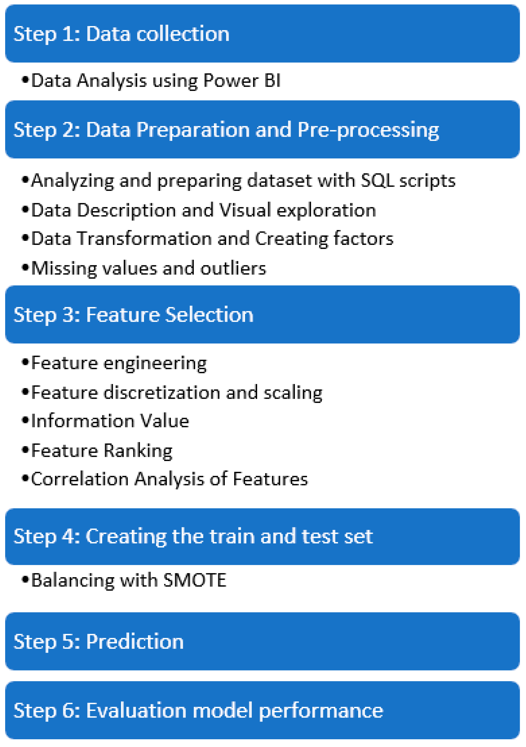
Figure 1 presents the steps of the methodology used in this research, where each step is explained in the following subsections.
3.1. Data Collection
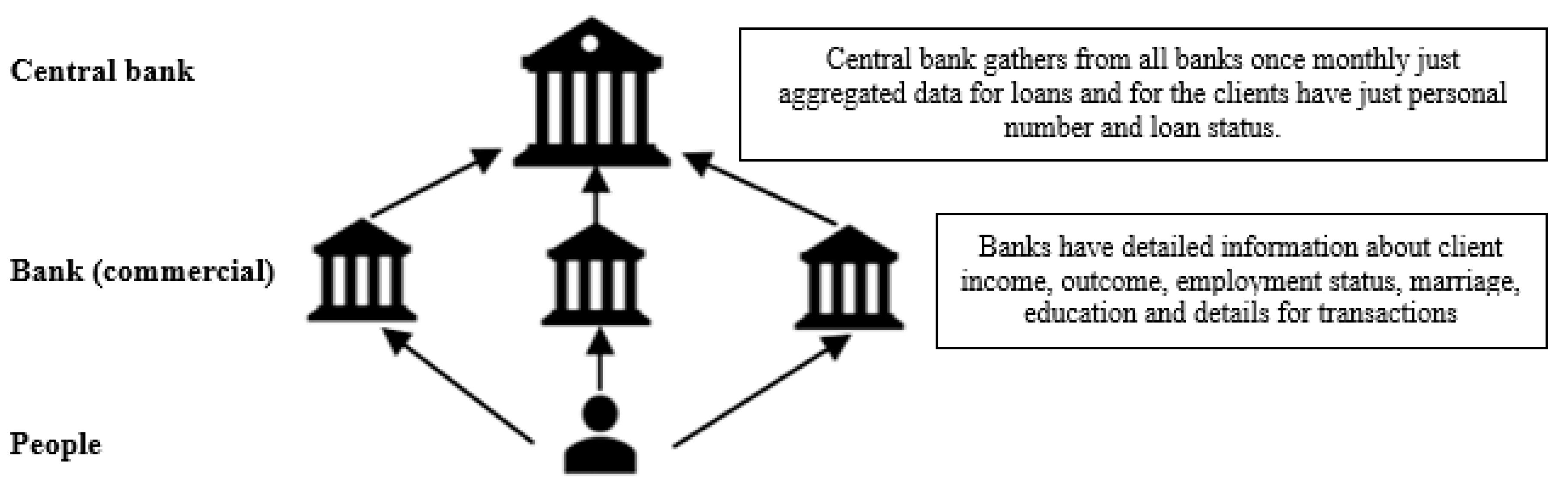
We use the dataset of the credit registry of the Republic of North Macedonia, which consists of around 1 billion entries, making it the biggest by size and by number of transactions in the central bank.
Initially, it consists of 52 financial and non-financial attributes, and all the private fields are anonymized for data confidentiality and General Data Protection Regulation (GDPR) during the experiments. The dataset is the central point for all the credits in the country, and it gathers data from all other commercial banks and saving houses (see
Figure 2). In this dataset, each entry represents a monthly status for each credit and credit card status for a given client.
This dataset is the biggest database in the central bank, and it fulfills most of the big data characteristics such as volume and velocity. There are a lot of validation controls when inserting the data, and the data quality is well controlled.
The credit registry dataset has the following information submitted by banks:
Client type (legal entity, person, households, etc.);
Identification of the client (personal identification number, tax number and activity if legal entity, head office, etc.);
Exposure by credit party (amount, structure, data of approval, delayed days, regular interest, interest rate level, type of interest rate, purpose, etc.);
Payment of liabilities;
Other data and information related to the type of collateral, type of impairment, purpose and characteristics of the credit exposure and/or the client;
Written-off claims.
Unique to this dataset is the fact that there is no information about income, spending, shopping habits, social media details and personal data for the clients and companies, only the general client behavior and credit status in all commercial banks in the country is present. The attribute category is being used for credit risk and scoring, and it classifies each client in one of the five predefined categories, which are marked as A, B, C, D, E. Category A is the best, it means there is the least risk, and every subsequent category is the next worst category, whereby category E is the worst (
DECISION on the Methodology for Credit Risk Management n.d.). The client’s category decision is made manually by the commercial bank officials, and in the central bank, all the transactional data are just aggregated and made available to every bank participating in the credit registry as a current and historical information about client’s credit score. In
Table 1, statistics of client distribution per category are represented.
The size of the credit registry database was around 1TB, but in the study, we used a subset of this dataset containing 1,000,000 rows, which represent status of 1,000,000 different credits only for individual (private) clients and their status (probability of default) in the planned date of finishing the whole payment of the loan. The dataset does not have an attribute if the client is able to repay the loan (risky) or not. We derived this attribute from the client’s category attribute in the whole dataset and found their worst category in which they was classified for more than 20% of the observed time. After getting the worst category for the client, we divided the first two categories, which are overdue on loan payments by more than 90 days in accordance with the Basel New Accord definition (
Oreski et al. 2012) and decision of the National Bank of Republic of North Macedonia (
DECISION on the Methodology for Credit Risk Management n.d.). Non-risky borrowers are marked with credit risk value 0 that means they will successfully make all the payments and the other risky borrowers with a value of 1 risk of default to fail making the required payments of the loan.
Advanced Analytics of Credit Registry Dataset with Power BI
To understand better the dataset and to visualize the data, we used Power Business Intelligence (Power BI). Using its capabilities for advanced analytics, we visualized attributes, their dependencies, trends and dependencies with additional data sources. For performing the analysis, we performed multiple stages including and additional calculated columns, measures and star schema model. After model design and relationships, we created multiple reports in a very efficient way, which unlike traditional tools is incomparably fast and powerful with modern capabilities for visualization, dependency and prediction, which helped us to inspect the dataset and to gain better knowledge. Our decision for Power BI was also influenced by its speed of data manipulation and analysis. The subset of the dataset that we analyzed was 13 GB in size when residing in structured query language (SQL) database, which in Power BI format reduced to 330 MB, since Power BI has its own format that is adapted to handle big data (
Doko and Miskovski 2020).
3.2. Data Preparation and Pre-Processing
Data pre-processing is an inevitable step for obtaining quality outcome from the knowledge discovery algorithm under consideration. Most of the next steps are done in many iterations to achieve the wanted results. Following are the initial steps that are done in the preprocessing process.
3.2.1. Preparing Data with SQL Scripts
Because the data source persisted in SQL, we used transact-SQL (TSQL) queries for operations for creating subsets of the original dataset where we decreased the number of attributes by removing unnecessary private information especially textual data (phone, address, etc.) and aggregated some numerical values. For every column, despite the implemented controls for inserting data, we checked for max values for numerical data, and for non-numeric columns, we checked the length of the content. We also created new columns derived from the dataset such as age from personal number, total number of successfully paid loans and joining with other tables used as metadata for the main table. After the operations in SQL, the dataset was prepared for the next phase, i.e., visual exploration in R Studio (
RStudio | Open Source & Professional Software for Data Science Teams n.d.).
3.2.2. Data Description and Visual Exploration
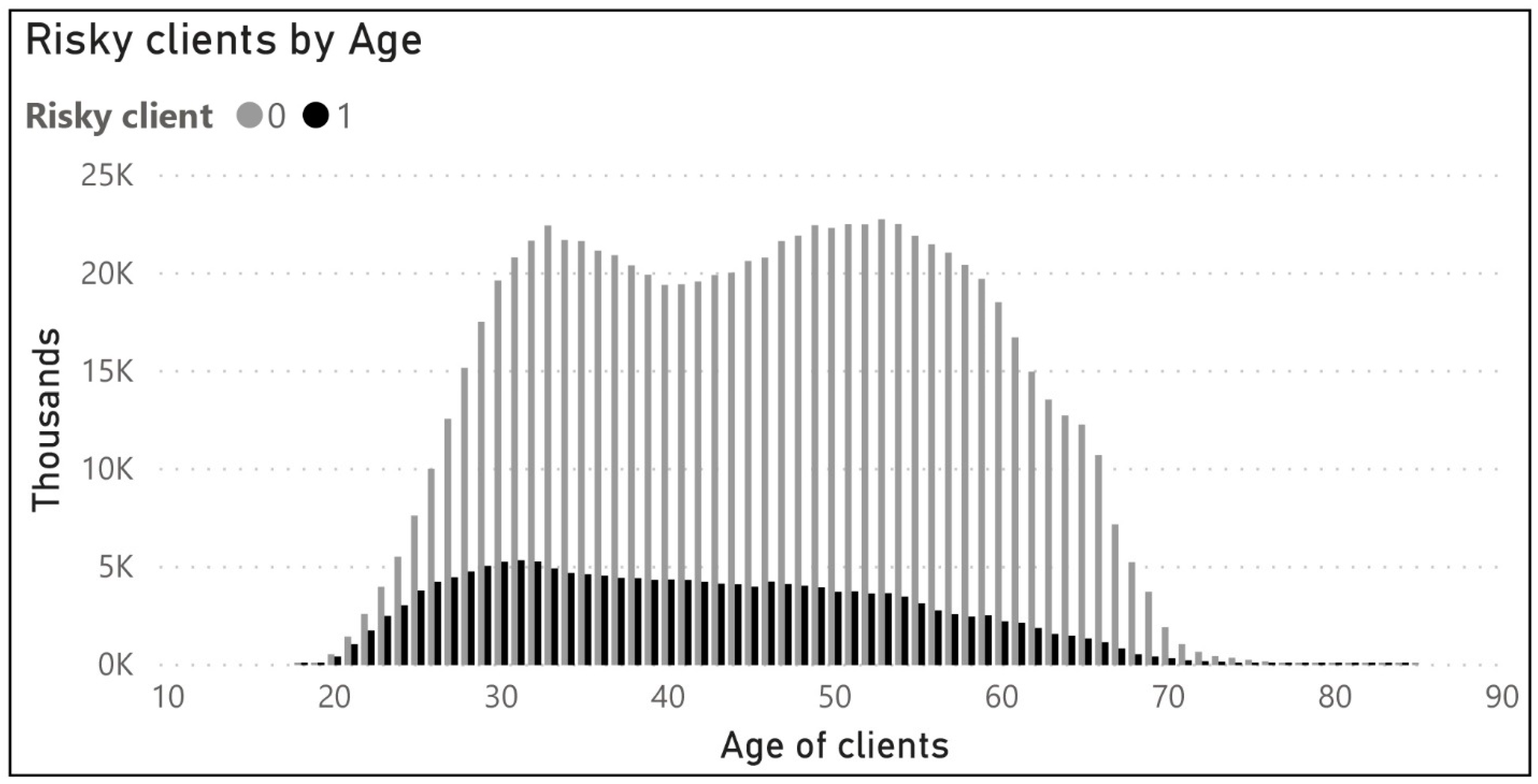
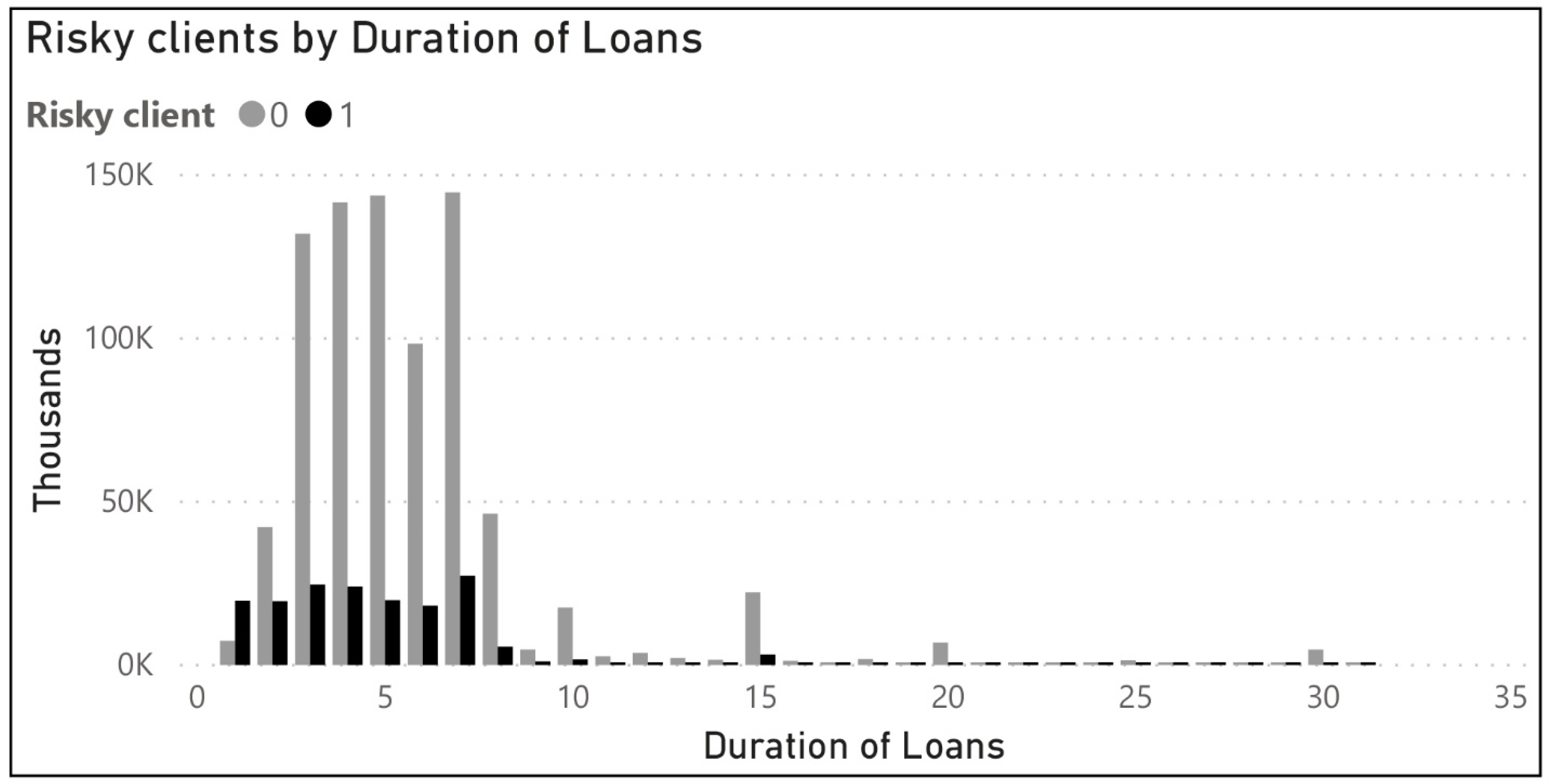
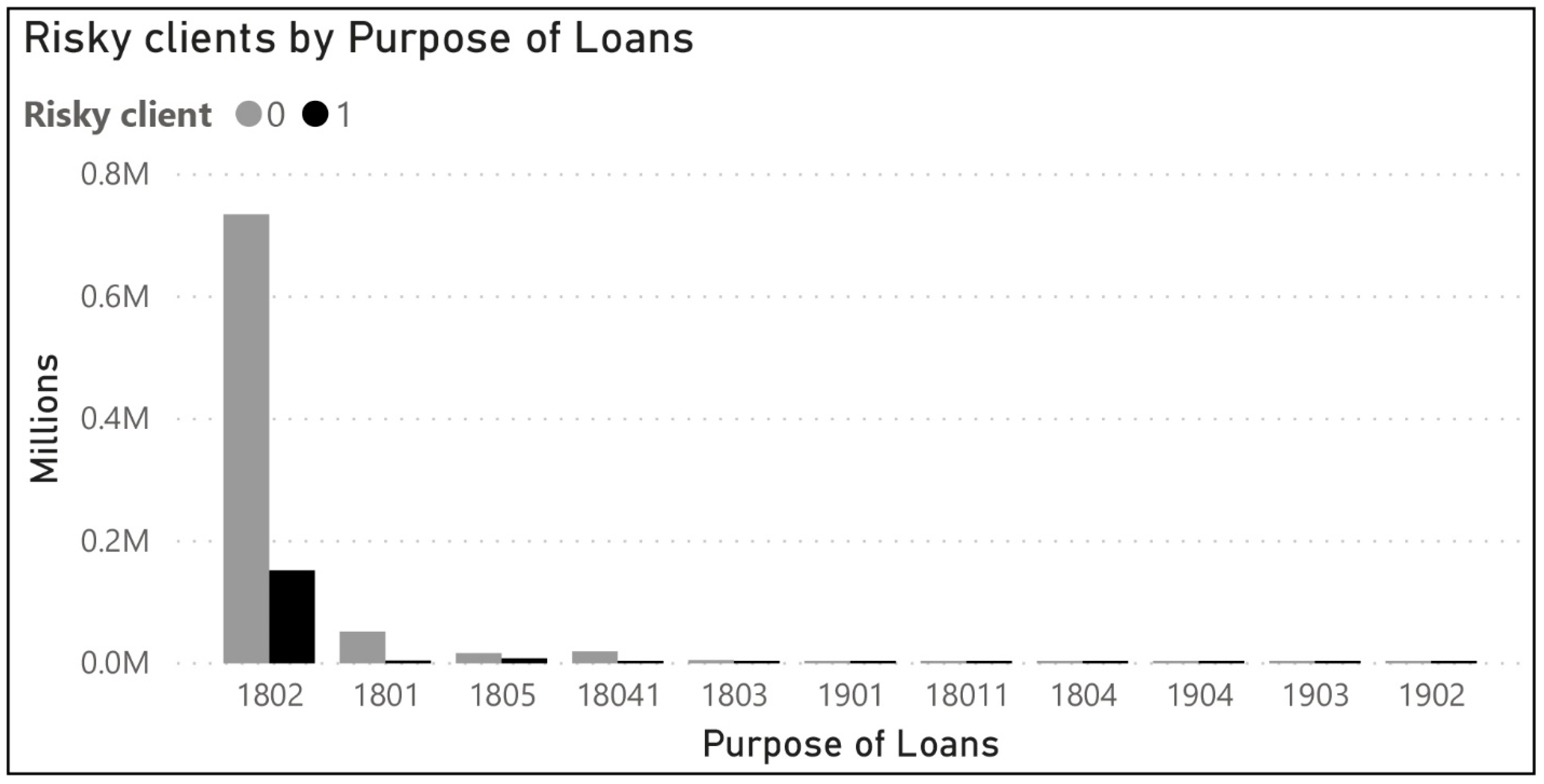
Gaining an initial understanding for the dataset is done with various exploration and visualization tools. Despite the Power BI, which we used mostly for the original dataset, for our 1,000,000 records, we used detailed exploration with existing R (statistical programming language) packages, which helped us to analyze the variable distributions, existing correlation between variables and outliers. By using plots, histograms, box plots and correlations between two variables, we became sure that the analysis can continue in next phase. According to
Figure 3,
Figure 4,
Figure 5 and
Figure 6, the initial visualizations provide more insights about distributions and risky clients, which helps understanding data for further analysis.
According
Table 2, the adjustable interest rate (P) is more represented in the dataset, then fixed interest rate (F) and, last, variable interest rate (V). Regarding the types of loans, annuity (A) loans are more represented in the dataset then (E), single returned loans.
3.2.3. Data Transformation and Creating Factors
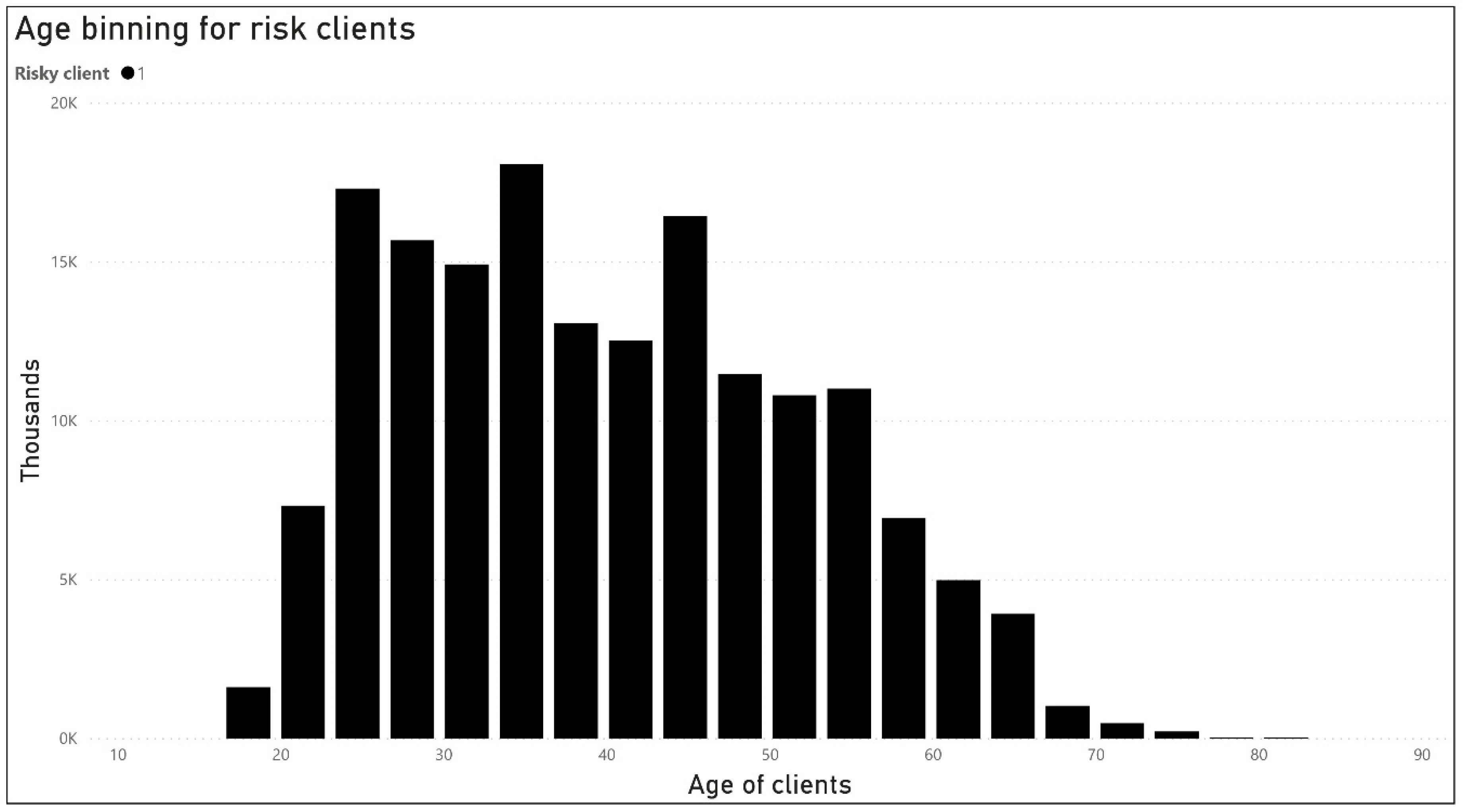
For categorical columns with a finite set of values, we created factors to represent categorical data. Factors are an important class for statistical analysis and for plotting. After creating factors for our categorical data, in our dataset, we had just factors and numerical data. As factors, we have the columns: bank size (small, medium, big), type of loan (annuity and single returned loans), interest rate (bins: 1, 2, 3, 4), type of interest rate (adjustable, fixed and variable interest rate), purpose (see
Table 2), age (see
Figure 7) and risky borrower (the dependent output variable with value 0 or 1). The numerical columns are number of loans, duration in years for the loan, the actual year of the loan, days delayed the payment and already successfully paid loans.
3.2.4. Missing Values Outliers
Null values in numerical columns are replaced with value mode. Because of changes in laws regulations of the credit registry, there are columns that are implemented later, and those missing values are zeroed. Because of the controlling methods on both sides of central and commercial banks, there were not any duplicates. After identifying the outliers with boxplot of the numeric attributes, they are removed to have a more reliable model. The prepared dataset after this phase does not have any missing data.
3.3. Feature Selection
3.3.1. Feature Engineering
To improve the efficiency of the model, with feature engineering, we augmented our dataset with the following columns:
BankSize—derived categorical column according to bank size code.
NumberofLoans—for every client we found the number of loans in the current reporting period.
SuccessfullyPaidLoans—represents the number of successfully paid loans in the history of the client.
DurationYearsLoan—derived column using the loan due date column.
Age—age is derived for individuals through their identification number.
In
Table 3, we have represented summary statistics for the derived columns using feature engineering.
3.3.2. Feature Discretization and Scaling
Because of the imbalanced nature of the dataset and to increase the value of predictors, we have implemented discretization, shown in
Figure 7. As compared in (
Zhang et al. 2020) for a credit scoring, dataset we used a quantile discretization method with 20 bins for age attribute and four bins for interest rate attribute. We also tried the optimal binning method for age with four bins, but the quantile discretization provided better results.
The attributes with continuous values are each on a different scale with high variances among them. For better visualization and impact in the model, continuous values columns are scaled to common scale.
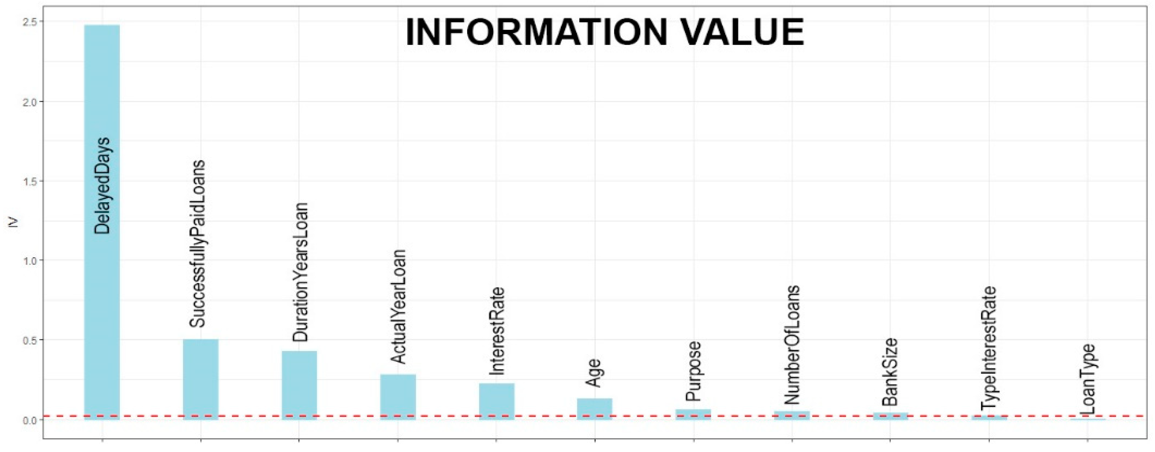
3.3.3. Information Value
To find the predictive power of each feature in relation to the dependent variable, we have used information value estimation, which is widely adopted in the credit scoring problems. With many iterations, we removed the attributes, which had unpredictive strength less than 0.02 (
Zdravevski et al. 2014).
These results were also confirmed when using random forest variable importance. The results in
Figure 8 show the predictive power analysis for relevant features, which showed an identical ordering as the information value analysis. The most important feature is delayed days, followed by number of successfully paid loans and duration of loans in years.
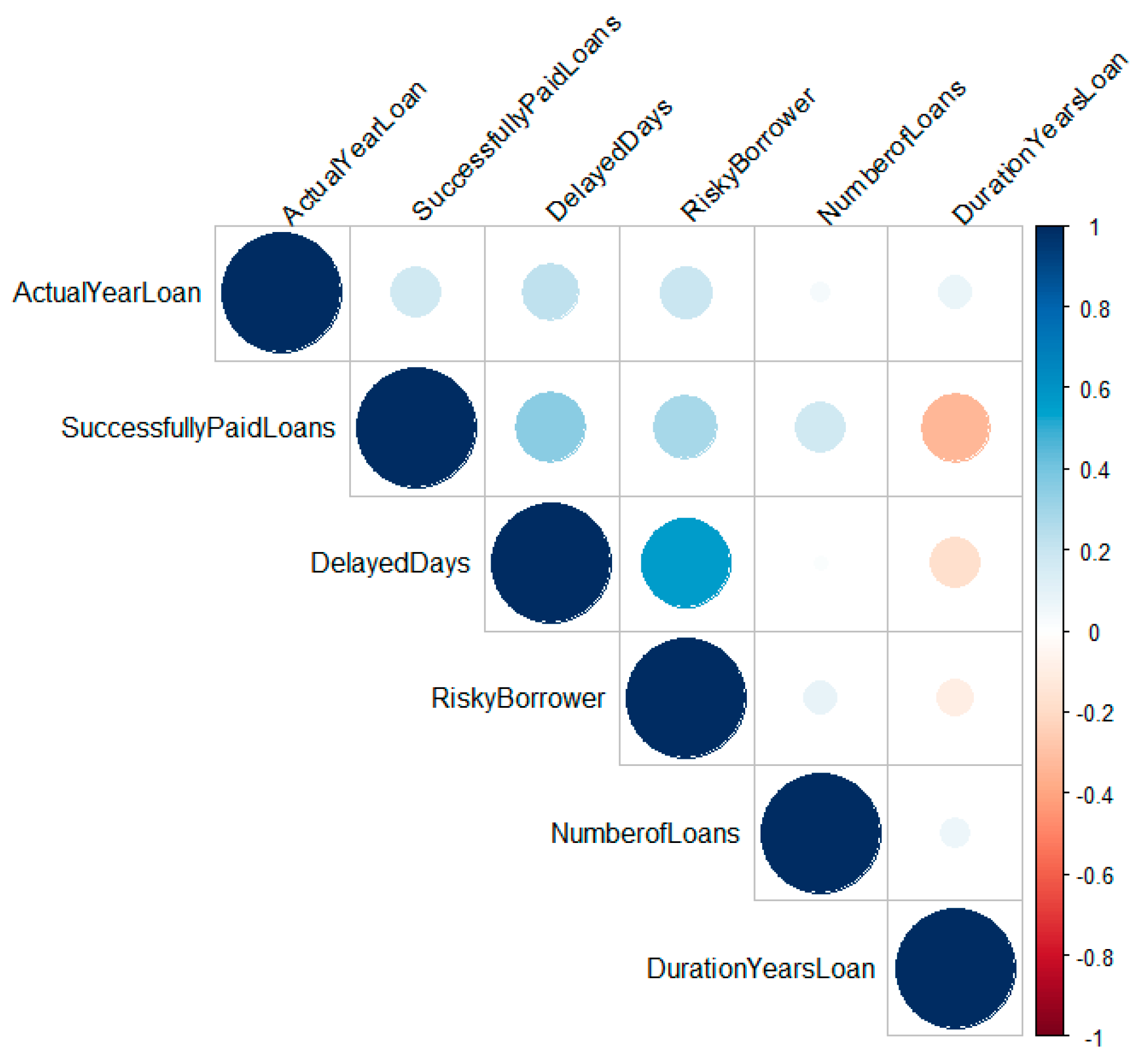
3.3.4. Correlation Analysis of Features
To avoid redundant or irrelevant features, which will disrupt the performances of the model, we have used correlation matrix using circles with appropriate coloring representing feature correlation. Correlations are found by using Pearson correlation test. The Pearson correlation has values between −1 and 1, where r = 1 or r = −1 represents a perfect linear relationship, and r = 0 represents no correlation between the variables.
According to
Figure 9, from the 11 columns in
Section 3.3.3, a higher correlation is found with days of delayed payment than with number of successfully paid loans and with current year of existing loan. Positive correlations will help for better predicting risky borrowers, and correlations with a score of less than 0.2 are not used in the data model. There were no negative correlations.
4. Results and Discussion
The splitting in training and testing dataset is done in the ratio 4:1, or the training dataset is 80% of data and the testing dataset is 20% of the data. After the initial splitting and visualizing data distribution, we found that both sets are very imbalanced.
For the training phase, we used the five most used algorithms for credit risk: logistic regression, which is parametric statistical model, decision tree, random forest, SVM and neural network. The effectiveness of the algorithm was checked with 10-fold cross validation to check the stability of the performing in practice on different sets of data.
To overcome the issue with the imbalanced dataset, which can lead to negative performance effects, we have used the synthetic minority oversampling technique (SMOTE) (
Chawla et al. 2002;
Shen et al. 2019) to test if it will generate better results. SMOTE will artificially increase the number of minority instances based on minority similarities in sample feature spaces. This will help to overcome the situation where the majority class will skew the results by a data bias towards the majority class. After many iterations and calibrations of the SMOTE function, we have reached a pretty balanced test set as displayed in
Table 4. SMOTE function artificially generates observations of minority class, and it balances the representation of both classes.
Because our dataset has both numerical and categorical attributes in our experiments, we have used versions with and without scaling to test whether it influences the results of the prediction.
Finally, we have the following four datasets on which different machine-learning models were built: imbalanced data without scaling, imbalanced data with scaling, balanced data with SMOTE without scaling, balanced data with SMOTE with scaling. Imbalanced datasets show better results than balanced ones, because SMOTE generates artificial rows, which in our dataset, did not help for getting better results.
In order to investigate the best model on the dataset, we have applied five machine-learning algorithms using the R programming language on the four datasets explained above. For neural networks, we have used the R nnet (
Nnet n.d.) package with 20 hidden layers, weight decay (regularization to avoid over-fitting) 0.001 and 20 iterations. As a tool, we used RStudio Desktop, Open Source Edition, Version 1.2.5042.
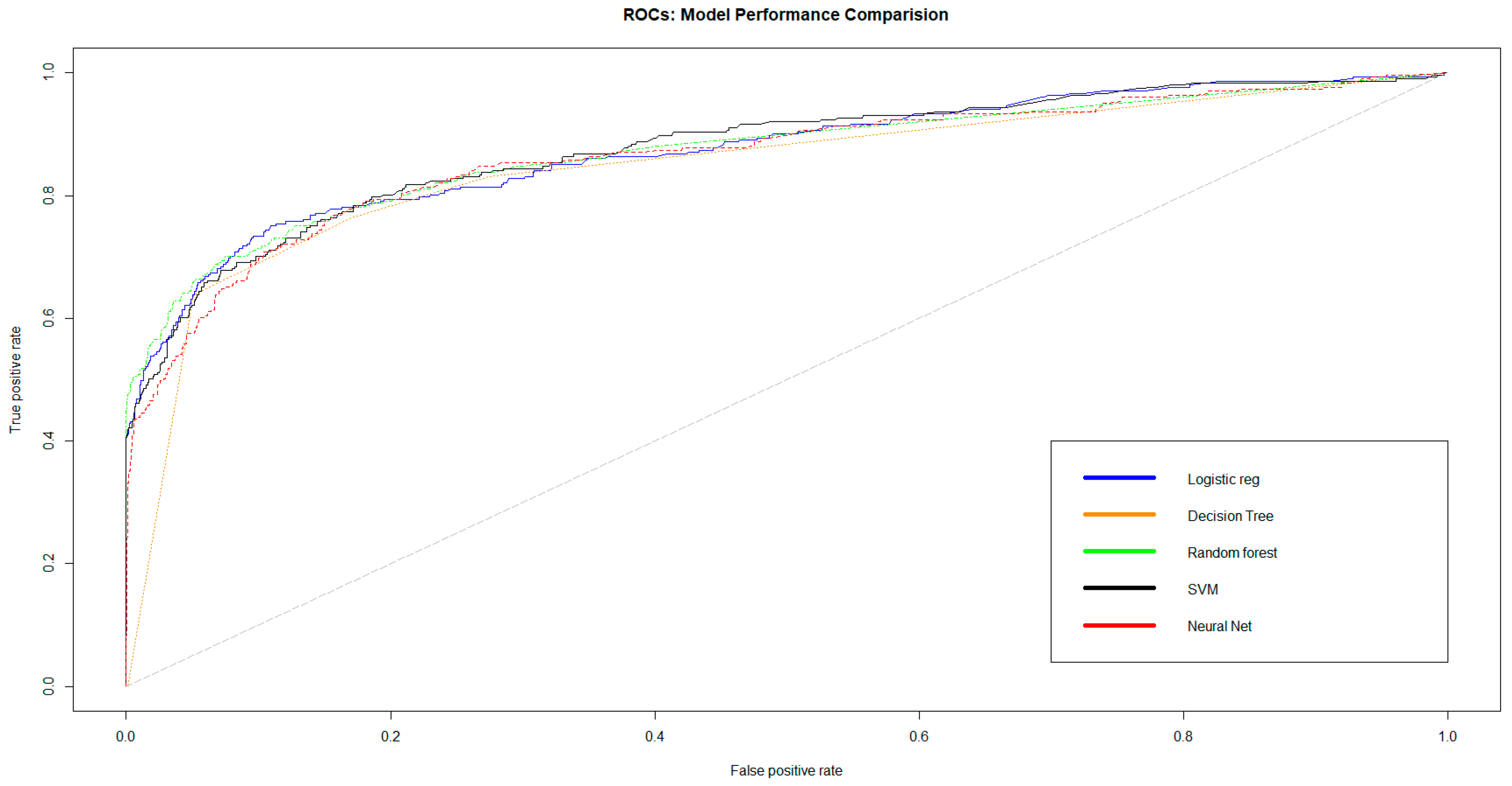
Figure 10 represents the ROC (
Bradley 1997) (receiver operating characteristic) curvefor all models trained on the balanced train set with SMOTE and without scaling. In
Table 5, we show the accuracy (accuracy = (TP + TN)/(TP + TN + FP + FN)), precision, recall and F1 score (function of precision and recall) for the five models on the same datasets. The results shown in
Table 5 are useful for imbalanced datasets, like in our dataset, where we have more samples of class 0 (non-risky borrowers) and less with class 1 (risky borrowers). Credit registry has a high class imbalance, because very few have defaulted, and the precision and recall are concerned with the correct prediction of the minority class, which is our aim.
Credit risk classification is sensitive and we do not want to miss on a borrower with risk going undetected (recall), but it is also important to know that the predicted one is true (precision). The precision–recall evaluation is more informative than the ROC plot when evaluating binary classifiers on imbalanced datasets, as it is our credit registry dataset (
Saito and Rehmsmeier 2015).
The results show that all the models are performing with high accuracy and precision on imbalanced data with feature scaling. In
Table 5, we are missing the balanced dataset with SMOTE and with scaling, because the results were not promising. The best models selected by F1 score are decision tree, random forest and linear regression. As shown in
Table 5, the results with feature scaling are very low, and the worst combination is when the data are balanced and scaled. The results obtained by comparing five machine-learning models also show better results compared with the existing papers on datasets of commercial banks. The results showed that the models performed best with high accuracy using imbalanced data with scaling and that the best algorithms are decision tree followed by random forest, logistic regression, SVM and neural network. Models also performed with high accuracy using imbalanced data without balancing, followed by using a balanced training set with SMOTE without scaling. The usage of feature scaling in our dataset showed that it has a minor effect on the results. In our case, it was because our attributes are almost within the same numerical ranges and do not have a big difference. Another interesting point is that balancing with SMOTE did not provide the expected improvements of the results as described above in the paper. In our opinion, this is because the ratio of our dataset between major and minor class was 1:2, which after all, is not a big difference. The dataset with the worst results was imbalanced and scaled; this may be because it adds noise on noise (balancing then scaling). Decision tree is also mentioned in our section for related work, and as such, it also draws the tree of conditions, which can also be valuable for credit approvals.
5. Conclusions
The presented methodology and results from this research could empower automated or semi-automated decisions for credit approval and will reduce the credit financial risk in the market. The dataset with its unique content will help new data science approaches to emerge, which will extract different insights and carry out better prediction, minimizing the credit and banks risks.
We have efficiently predicted borrowers’ credit risk from the credit registry dataset using historical data for all loans in all banks. Besides the methodology that we suggest and the models that we evaluate, our dataset is different from other commonly used datasets from banks because it is a real credit registry dataset from a central bank, and the data differ because they are aggregated for loans, and there are no data about client income, outcome, employment status and details for transactions. Our dataset resides in the central bank, which has historical data for all the client behaviors of the country and has more potential to predict the credit risk because of the huge amount of information from all the commercial banks. On the other hand, the drawback of our dataset is the unavailability of client personal information such as salary and spending transactions.
This proposed research can be an additional source of valuable information, which will help banks to make proper decisions for granting credit. After the operationalization of this model in the central bank, the commercial banks need only to send the personal number of the client, and the model will return its prediction about the risk using historical data and the client’s behaviors in all the banks in the country, thus providing informed decisions gained from big centralized data sources. We believe that by using this approach, banks will have huge benefits, i.e., instead of just getting historical data for the client from the central banks, they can also get a prediction about credit risk for a given client. Based on our model, to have accepted credit, the client must not have delayed payments for previous loans and should have successfully paid any previous loans, and age should not be in the bins with higher risk.
As a drawback, our paper uses only one dataset, and all countries have a similar dataset, which can vary by its requirements, laws and roles. Based on the financial roles of North Macedonia, our described methodology can be easily implemented in other countries. Another drawback is that there is not any research that uses data from credit risk, and we were unable to carry out such a comparison. There only papers that use the known public datasets of banks are, for example, German, Australian and Japanese datasets. However, we leave this for future work and analysis. Besides that, in the future, we plan to augment the dataset using other open datasets, to experiment the prediction with multiclass classification and to undertake time-series forecasting prediction for the borrower’s status after some months or years.
Although the described models in the manuscript produced good accuracy, we will compare the predictive analytics with deterministic artificial intelligence methods to compare for improvements. Our future work will include experimenting deterministic artificial intelligence methods, which can provide better accuracy in lower execution time (
Smeresky et al. 2020). To minimize the uncertainty of our model, we will re-model it by re-parametrizing the problem into a form to minimize the variance and uncertainty (
Sands 2020).


