Article

Quanto Pricing beyond Black–Scholes

1
Department of Computer Science and Mathematics, Munich University of Applied Sciences, Lothstr. 64, 80335 Munich, Germany
2
Department of Statistics, Ludwig-Maximilians-Universität München, Akademiestrasse 1/I, 80799 Munich, Germany
*
Author to whom correspondence should be addressed.
J. Risk Financial Manag. 2021, 14(3), 136; https://doi.org/10.3390/jrfm14030136
Submission received: 16 February 2021 / Revised: 3 March 2021 / Accepted: 12 March 2021 / Published: 23 March 2021
(This article belongs to the Special Issue Structured Financial Products and Derivatives)

Abstract

:
Since their introduction, quanto options have steadily gained popularity. Matching Black–Scholes-type pricing models and, more recently, a fat-tailed, normal tempered stable variant have been established. The objective here is to empirically assess the adequacy of quanto-option pricing models. The validation of quanto-pricing models has been a challenge so far, due to the lack of comprehensive data records of exchange-traded quanto transactions. To overcome this, we make use of exchange-traded structured products. After deriving prices for composite options in the existing modeling framework, we propose a new calibration procedure, carry out extensive analyses of parameter stability and assess the goodness of fit for plain vanilla and exotic double-barrier options.

1. Introduction

Recent events in Japan, starting with the 2012 general election that made Shinzo Abe prime minister, brought the country of deflation and economic stagnation back into the focus of global investors. The main goals of the Abe administration were bringing up inflation to 2%, weakening the Japanese yen and pushing for more growth. Therefore, it is only natural to ask how foreign investors can get exposure to the Japanese equity market in form of, say, its major index, the Nikkei 225. Conventional choices would be to either directly invest into the index or to pursue a riskier option strategy. Both approaches may, however, be hampered by the effects of “Abenomics,” namely, that investors may benefit from rising equity prices but a weakening yen may offset the profits. A possible solution to this problem is to resort to quanto options, i.e., derivatives where the exchange rate at maturity has been fixed upfront.
To allow for such features in classical option pricing, not one but two asset prices need to be modeled, namely, that of the equity index and that of the foreign exchange (FX) as well the dependence structure between the two. Although quanto derivatives have gained popularity, results on quanto pricing are rather scarce. Standard approaches, such as Derman et al. (1990); Baxter and Rennie (1996) or Wilmott (2006), assume two-dimensional Black–Scholes-type markets, with recent extensions allowing for stochastic volatility (Dimitroff et al. (2009); Branger and Muck (2012) and Park et al. (2013)) and dynamic correlation (Teng et al. (2015)). However, all these models rely on the assumption that the underlying assets are governed by a multivariate Brownian motion, which fails to capture the omnipresent heavy-tailedness and asymmetric dependence in asset returns. Kim et al. (2015) were the first to leave this framework by specifying normal tempered stable (NTS) processes to drive asset dynamics. These represent a subtype of the rich Lévy class, which has been in the focus of market modeling since the early work of Eberlein and Keller (1995) and Eberlein et al. (1998). In particular, NTS processes were constructed in Barndorff-Nielsen and Levendorskii (2001) by certain time-changed Brownian motions and have since then been investigated especially in the context of portfolio analysis and option pricing, cf. Barndorff-Nielsen and Shephard (2001); Kim et al. (2012) or Fink et al. (2019). In recent work, Ballotta et al. (2015) formulate a general multivariate Lévy framework for combined equity and FX markets to investigate model-implied correlations based on futures and plain vanilla options.
Kim et al. (2015) introduced the NTS model to price quanto options but, except from an illustrative application using synthetic prices, did not provide any empirical validation. As they point out, exchange-traded quanto options—especially beyond plain-vanilla contracts—are hard to obtain and price histories of OTC trades are, per definition, not available. Here, we fill this gap and conduct an extensive empirical investigation of the NTS quanto model. To do so, we consider two types of exchange-traded warrants, which are a special class of retail-structured products (RSPs), namely, plain vanilla options and exotic double-barrier options. For these derivatives, as detailed in Section 3 below, market makers provide not only constant liquidity but also let us make use of exchange-recorded daily closing prices to compare different quanto pricing models beyond vanilla calls and puts. As conjectured in Kim et al. (2015), our results show that the NTS model clearly dominates the Gaussian framework.
The paper is structured as follows. Section 2 presents the classical Black–Scholes-type setup and the newly introduced NTS framework of Kim et al. (2015), stating model assumptions and pricing formulas. Furthermore, estimation results using historical return data are presented and parameter restrictions for the NTS setup are motivated. The data we use are described in Section 3. Preliminary results from fitting the pricing formulas to real market prices are presented in Section 4. Although the fits look very much in favor of the NTS assumption, we will show that parameter identification and stability can be an issue. To overcome this, we theoretically extend the NTS model in Section 5 and provide pricing formulas for composite (compo) options on the stock and the FX rate individually. Using these price representations and combining historical estimation with risk-neutral calibration, we address stability and identification issues while leaving the main advantages of the NTS model untouched. A brief summary closes the paper.1

2. The NTS Framework for Quanto Options

Following the theoretical setup of Kim et al. (2015), we model quanto options under two different assumptions: a two-dimensional NTS framework, the object of interest, and, for reference purposes, the classical Black–Scholes-type setting. For both setups, we assume the existence of two riskless rates: Let r d 0 and r f 0 be the instantaneous interest rates for the domestic and foreign currency, respectively. In particular, there is one riskless (domestic) bank account denoted by
B = { B ( t ) } t 0 with B ( t ) = exp { r d t } , t 0 .
In our empirical study below, the domestic currency shall be the euro (EUR) and the foreign currency the Japanese yen (JPY).2 Furthermore, we assume the existence of two tradable risky assets:
V = { V ( t ) } t 0
denotes the price process of an equity-type asset in the domestic currency (the Nikkei 225 index converted into EUR), while
exp { r f · } F = { exp { r f t } F ( t ) } t 0
describes the (tradable) exchange rate process from the domestic (EUR) to the foreign currency (JPY); i.e., at time t 0 , an investor gets for one unit of foreign currency (JPY) F ( t ) units of the domestic numéraire (EUR). We want to stress the importance of the factor exp { r f t } : Any investment in the foreign currency would incur an interest rate payment of r f . So, while F itself shall be the FX spot rate, it can only be traded via the foreign cash bond exp { r f · } F . By combining both, we obtain the price process of the equity asset in the foreign currency (the Nikkei 225 index in JPY), given by
N = { N ( t ) } t 0 = V ( t ) F ( t ) t 0 .
Remark 1 (Model summary).
(i) Below, EUR will be our domestic currency as we consider quanto options traded on the Frankfurt Exchange in EUR. N then denotes the Nikkei 225 in the foreign currency JPY (from a European investors perspective), although the JPY is actually the local currency for the Nikkei 225.
(ii) Even though there are two riskless interests rates in our model, r d and r f , there is only one riskless bank account B which is denoted in the domestic currency. A foreign counterpart would be subject to exchange-rate risk and return exp { r f · } F .
Given this general market framework, we first specify the (simpler) Black–Scholes-type setting making the following assumptions:
Assumption 1
(Black–Scholes setting, see Kim et al. (2015), Section 3.1). Let W = ( W X , W ¯ Y ) = { ( W X ( t ) , W ¯ Y ( t ) ) } t 0 be a two-dimensional standard Brownian motion with independent marginal processes. To construct straightforwardly tractable, dependent processes for the equity asset, V, and the FX rate, F, let μ X , μ Y R , σ X , σ Y > 0 and ρ [ 1 , 1 ] . We specify
W Y : = ρ W X + 1 ρ 2 W ¯ Y ,
so that C orr ( W X ( t ) , W Y ( t ) ) = ρ t for t 0 , and, with V ( 0 ) > 0 and F ( 0 ) > 0 , assume the following dynamics under the real-world measure P for t 0
V ( t ) = V ( 0 ) exp { μ X t + σ X W X ( t ) } and F ( t ) = F ( 0 ) exp { μ Y t + σ Y W Y ( t ) } .
To price quanto options, the above setup needs to be arbitrage-free with the usually considered class of admissible trading strategies see Delbaen and Schachermayer (1994) thus allowing the construction of a suitable equivalent martingale measure. Since we have two tradable assets and two sources of risk, both given by Brownian motions, we have the following theorem.
Theorem 1
(see Kim et al. (2015), Section 3.1). Let Assumption 1 hold with | ρ | < 1 . Then, there exists a unique equivalent measure Q under which
V ( t ) = V ( 0 ) exp { r d t σ X 2 2 t + σ X B X ( t ) } , F ( t ) = F ( 0 ) exp { ( r d r f ) t σ Y 2 2 t + σ Y ρ B X ( t ) + σ Y 1 ρ 2 B ¯ Y ( t ) } ,
for t 0 and where B = ( B X , B ¯ Y ) = { ( B X ( t ) , B ¯ Y ( t ) ) } t 0 is a two-dimensional standard Brownian motion with independent marginal processes. Furthermore, the discounted tradable assets { exp { r d t } V ( t ) } t 0 and { exp { ( r d r f ) t } F ( t ) } t 0 are Q -martingales.
Let T > 0 , then the price, C t ( K , T ) , of a European quanto call option on N ( T ) with strike K > 0 at time 0 t T is given by
C t q u a n t o ( K , T ) = exp { r d ( T t ) } E Q [ F f i x ( N ( T ) K ) + | F t ] = F f i x e ( r f r d + σ Y 2 ρ σ X σ Y ) ( T t ) N ( t ) Φ ( d 1 ) e r d ( T t ) K Φ ( d 2 )
where
d 1 = log ( N ( t ) / K ) + ( r f + σ Y 2 ρ σ X σ Y + 1 2 [ σ X 2 2 σ X σ Y ρ + σ Y 2 ] ) ( T t ) [ σ X 2 2 σ X σ Y ρ + σ Y 2 ] T t , d 2 = d 1 [ σ X 2 2 σ X σ Y ρ + σ Y 2 ] T t .
Here ( F t ) 0 is the (augmented) filtration generated by V and F which we can assume to satisfy the usual conditions of right-continuity and completeness.
Having set up our reference model, we turn to the NTS setting of Kim et al. (2015), the object of interest in our empirical study.
Assumption 2
(NTS market setting, see Kim et al. (2015), Section 3.2). Let T = { T ( t ) } t 0 be a tempered stable subordinator, i.e., an a.s. increasing Lévy process with characteristic function
E exp { i u T ( t ) } = exp 2 t θ 1 α 2 α ( θ i u ) α 2 θ α 2 , u R , t 0 ,
with α ( 0 , 2 ] and θ > 0 . For a two-dimensional standard Brownian motion B = ( B X , B Y ) = { ( B X ( t ) , B Y ( t ) ) } t 0 with correlated marginal processes, independent of T , construct a two-dimensional NTS process ( X , Y ) = { ( X ( t ) , Y ( t ) ) } t 0 by
X ( t ) Y ( t ) = μ X μ Y t + β X β Y [ T ( t ) t ] + σ X 0 0 σ Y B X ( T ( t ) ) B Y ( T ( t ) )
with μ X , μ Y , β X , β Y R , σ X , σ Y > 0 and C orr ( B X ( t ) , B Y ( t ) ) = ρ t , t 0 , ρ [ 1 , 1 ] . We write
( X , Y ) NTS 2 α , θ , μ X μ Y , β X β Y , σ X σ Y , 1 ρ ρ 1 .
Furthermore, with V ( 0 ) > 0 and F ( 0 ) > 0 , we assume the following dynamics for our tradable assets under the real-world measure P for t 0 :
V ( t ) = V ( 0 ) exp { X ( t ) } and F ( t ) = F ( 0 ) exp { Y ( t ) } .
It is well known that subordinated Lévy processes are again of the Lévy type. Therefore, all measure changes under which the Lévy property is invariant basically modify the deterministic drift and the jump intensity.3 Choosing such a measure change (in particular one of the Esscher transform type, see Gerber and Shiu (1994) and Eberlein et al. (2009) for more background) and defining the functions
w X : , θ β X σ X 2 2 λ X 🟉 β X 2 θ 1 α 2 α θ β X λ X 🟉 σ X 2 2 α 2 θ α 2
and
w Y : , θ β Y σ Y 2 2 λ Y 🟉 β Y 2 θ 1 α 2 α θ β Y λ Y 🟉 σ Y 2 2 α 2 θ α 2 ,
Kim et al. (2015) proved the following theorem.
Theorem 2
(Kim et al. (2015), Section 3.2 and Theorem 3.1). Let Assumption 2 hold with | ρ | < 1 and suppose that there are
λ X 🟉 < θ β Y σ Y 2 2 and λ Y 🟉 < θ β Y σ Y 2 2 ,
such that
μ X r d + w X ( λ X 🟉 ) = 0 and μ Y r d + r f + w Y ( λ Y 🟉 ) = 0 .
Then, there exists an equivalent measure Q under which
V ( t ) = V ( 0 ) exp { ( r d w X ( λ X 🟉 ) ) t + X ( t ) } , F ( t ) = F ( 0 ) exp { ( r d r f w Y ( λ Y 🟉 ) ) t + Y ( t ) } ,
for t 0 , with
( X , Y ) NTS 2 α , θ , λ X 🟉 λ Y 🟉 , β X + λ X 🟉 β Y + λ Y 🟉 , σ X σ Y , 1 ρ ρ 1 .
The discounted tradable assets { exp { r d t } V ( t ) } t 0 and { exp { ( r d r f ) t } F ( t ) } t 0 are Q -martingales.
Let T > 0 , then the price, C t ( K , T ) , of a European quanto call option on N ( T ) with strike K > 0 at time 0 t T is given by
C t q u a n t o ( K , T ) = exp { r d ( T t ) } E Q [ F f i x ( N ( T ) K ) + | F t ] = e r d ( T t ) F f i x K 1 + ζ 2 π N ( t ) ζ e ζ ( r f w X ( λ X 🟉 ) + w Y ( λ Y 🟉 ) ) ( T t ) F 1 2 π log K N ( t ) ,
where
F ( x ) = R e 2 π i u x e i u ( r f w X ( λ X 🟉 ) + w Y ( λ Y 🟉 ) ) ( T t ) ( i u ζ 1 ) ( i u ζ ) E e ( i u ζ ) Z ( T t ) d u ,
with Z = X Y and ζ R , such that the appearing moment generating function exists. Again, ( F t ) 0 is the augmented filtration generated by V and F and satisfying the usual conditions of right-continuity and completeness.
As pointed out in Kim et al. (2015), the call-price formula (derived by classical Fourier pricing methods, see Carr and Madan (1999)) can be efficiently evaluated by the Fast Fourier Transform.
We close this section by presenting parameter estimates using daily return data as shown in Figure 1. The data cover the period 4 January 2000 to 15 April 2013.4 The annualized parameter estimates, obtained by maximum likelihood and based on inversion of the characteristic functions of the NTS setup, are reported in Table 1.5
For all time series, the goodness of fit, measured in terms of both the log-likelihood and the model-selection criteria AIC and BIC strongly favor the NTS over the Black–Scholes model. Note that both market models produce a modest positive correlation. However, when interpreting this effect, we need to be aware that V describes the Nikkei 225 in EUR not in JPY. Given that, in the Gaussian case,
C orr log N ( t ) N ( t 1 ) , log F ( t ) F ( t 1 ) = σ X ρ σ Y σ X 2 2 σ X σ Y ρ + σ Y 2 ,
our parameter estimates imply a correlation of 0.4691 between the log returns of N and F, i.e., the Nikkei 225 (in JPY) tends to decline when the JPY appreciates, a relationship we expect given the export-orientation of the Japanese economy.
The estimate for the tail parameter, α , of 1.30 with 95%-confidence interval [1.07,1.45] indicates a considerably heavier and distinctly different tail behavior compared to the Gaussian assumption. Furthermore, the estimated skewness parameters, β , indicate a milde but significant skewness in the distributions. Figure 2, showing the estimated densities and log-densities implied by both models for V, F and N, illustrates both phenomena. As will be discussed in Section 4, the fact that the Black–Scholes model cannot capture the empirically observed fat-tailedness has serious implications when pricing double-barrier options.
It remains to explain why we impose parameter restrictions to α and θ . Consider simulated paths of V / F with varying α and θ , shown in Figure 3. (The exact simulation procedure will be explained in Section 4 below). As we can see, small values for the tempering parameter θ produce highly unrealistic sample paths with very large jumps. Furthermore, tail parameters α below one lead to paths with finite variation (see Section 2 of Kim et al. (2015)). Finally, if both are taken too small or if θ is very large, numerical instabilities can arise.

3. Data on Retail Structured Products

Next, we describe the data used in the empirical investigation. As already pointed out in Kim et al. (2015), classical quanto options, like calls and puts, are rarely traded on official exchanges.6 Per definition, OTC trades are not recorded by financial data providers and, thus, not available for empirical analyses. The data situation differs, however, when turning to retail structured products (RSPs). Looking just at the German market (being one of the largest RSP markets in the world), several banks and issuers provide quanto structures to be tradable at retail exchanges, where issuers are usually committed to continuously quote bid and offer prices that can be accessed.
Focusing on Nikkei 225 quanto RSPs, Société Générale appears to be the dominating issuer in Germany in terms of available products.7 For this reason and to avoid possible differences between issuers (see Remark 2 below), we focus on the French investment bank’s products.
Our data set consists of 29 quanto call options on the Nikkei 225 (traded in EUR) and 363 digital knock-out (KO) options with upper and lower barriers also referred to as inline options or double-barrier options, respectively. The later pay a fixed amount in EUR (10 EUR in our case) at maturity if the Nikkei 225 (in JPY) based on tick-by-tick observations has never touched or violated any of the barriers. Therefore, they can basically be classified as quanto KO options. In addition, we have 18 compo FX options (11 calls, 7 puts) on EURJPY and 20 compo calls on the Nikkei 225, both types with EUR as a base currency. The sample period we consider ranges from 16 April 2013 (issue date) to 15 September 2014 for the plain vanilla options and from 19 June 2013 to 15 September 2014 for the KO warrants, covering a total period of 17 months—a sample size that is in line with similar studies (e.g., Guillaume (2013)). After removing trading days where recordings are missing, we are left with a total of 354 daily closing-price observations (see Figure 4).8
Since the Japanese markets are closed at the time the option prices are recorded, we rely on the price of a quanto Nikkei 225 open-end-tracker issued and priced by Société Générale. This American product gives the buyer the right to exercise it with a three-month notice period every year on November 26 and to receive the Nikkei 225 close on this Japanese trading day (ratio 100:1). The spread of this product is quite tight and one can expect these kind of RSPs not to contain much margin for the issuer (see Remark 2). As a direct consequence, its pricing should closely resemble Société Générale’s proprietary Nikkei 225 indication. As for the EURJPY rate, we compare several issuers’ quanto and compo Nikkei 225 tracker and implicitly derive the (mean) FX rate.9
Remark 2.
As we are looking at RSPs (plain vanilla and double-barrier options) there are some potential sources for a systemic bias from the ’fair model price’.
(i) 
Credit risk: All products are basically a type of bearer bonds and, thus, are expected to include counterparty risk. Therefore, one would assume, considering only this effect, tradable prices to be somewhat lower than those coming from classical option pricing models as investors would want to be compensated for taking on default risk.
(ii) 
Issuer’s PnL: Issuers intend to profit from structuring and pricing RSPs which is reflected in the overpricing- and the lifecycle-hypothesis. Overpricing means a certain margin is charged on top of the model price (see Chen and Kensinger (1990) and Chen and Sears (1990) for the US retail market and Wilkens et al. (2003) for Germany). According to the lifecycle-hypothesis, this charge tends to decrease over time as the issuer presumably wants to profit from initial investors selling back later (see Stoimenov and Wilkens (2005)).
(iii) 
Dividends: The Nikkei 225 is a price index and, thus, does not account for dividends. Therefore, all else being equal, the index would decrease over time through this effect. The chosen market setups (Black–Scholes and NTS alike) do not account for such dividends.
However, the bias may not be dramatic as these three effects tend to partially offset each other: Sources ( i ) and ( i i i ) cause model prices to be higher than the real market prices, while neglecting ( i i ) will induce lower model-implied quotes.

4. Naive Model Calibration Using Quanto Options

As stated above, our goal is to empirically compare the NTS assumption with the classical Gaussian benchmark. The later is known to be deficient, especially when it comes to more exotic payoffs, as significant risks, like jump or tail risk, might be underpriced. To assess model adequacy, we conduct two types of empirical comparisons: the in-sample fit, obtained by calibrating parameters to classical vanilla options, and the out-of-sample fit via pricing exotic double-barrier derivatives.
We first use vanilla options to calibrate the parameters for each trading day, compare the models’ in-sample-fit, and then calculate delta-based forecasts to assess parameter stability by plugging in yesterday’s parameter values into today’s pricing formula.10 We follow Teng et al. (2015) and minimize the relative mean square error (RelMSE) to calibrate the models due to the relative large differences in absolute option prices, i.e., we chose the respective parameters collected in the vector Θ t 🟉 by minimizing11 the daily RelMSE between market and model prices, i.e.,
Θ t 🟉 = argmin Θ RelMSE ( Θ ) t : = argmin Θ 1 n t i = 1 n t P t model ( K i , T i | Θ ) P t market ( K i , T i ) 2 P t market ( K i , T i ) ,
where n t denotes the number of observed prices on day t. As starting points for the Black–Scholes pricing we choose the historical volatilities and correlation of the Nikkei 225 in EUR and the JPYEUR exchange rate obtained by maximum likelihood estimation (see Table 1). For the NTS calibration, we start with the implied Black–Scholes volatilities and correlation and set the other initial values additionally to α = 1.5 , θ = 25 and μ X = μ Y = β X = β Y = 0 . The semi-analytic Formula (3) is approximated by the Fast Fourier Transform algorithm. To avoid any numerical instabilities for α 2 , we restricted ourselves to α [ 1 , 1.95 ] { 2 } and θ [ 20 , 200 ] (see the discussion at the end of Section 2).
For the second comparison, we use the obtained daily parameters and assess the out-of-sample model fit by pricing the KO warrants described in Section 3. This, however, is not straightforward, since pricing such barrier options amounts to knowing the distribution of the running minimum and maximum of the underlying price process. For Black–Scholes-type settings, this problem has been considered by Kunitomo and Ikeda (1992) and Geman and Yor (1996), so that useful formulas for implementation are available.
For general Lévy markets (as the NTS setup) several solutions are possible12 but there is no simple analytic formula. Besides classical simulation-based Monte Carlo methods, which will be used here, other numerical or semi-analytical approaches include partial integro-differential equations (PIDEs) and Fourier methods.13 As NTS processes are partially generated by certain time-changed Brownian motions, the work of Escobar et al. (2014) is also closely related to our setup, but differs in that our subordinator, appearing in the NTS definition, is a jump process.
All these studies focus on continuous barriers. In reality, a continuous observation is impossible. In fact, the considered KO options observe the barrier only when Nikkei 225 prints are available, which is every 15 s during the five-hour trading day. Therefore, when using PIDE or Fourier methods, some kind of continuity correction would be necessary as well (see Broadie and Glasserman (1997) for the Gaussian case). To avoid this, we rely on simulation-based pricing which suffices for our objectives. The general idea is as follows: For a double-barrier option with maturity T, upper barrier K u and lower barrier K l , we simulate M sample paths, { N ˜ i ( t ) } 0 t T , i { 1 , , N } , under Q and approximate, for t T ,
KO t ( K u , K l , T ) = exp { r d ( T t ) } E Q [ 10 EUR × 1 { K l < min t T N ( t ) , max t T N ( t ) < K u } | F t ] 10 EUR × exp { r d ( T t ) } M i = 1 M 1 { K l < min t T N ˜ ( t ) } 1 { max t T N ˜ ( t ) < K u }
under the restriction that none of the barriers have been touched until t 0 .14 The main challenge here (besides the computational burden) is to simulate from the NTS distribution. In the light of (2) and an application of classical Euler–Maruyama schemes, this basically boils down to obtaining realizations from the driving tempered stable subordinator. Potential solutions include sampling by an infinite series representation, as in Bianchi et al. (2010), or numerically inverting the cumulative distribution function (which can itself be obtained by Fourier transformation of the characteristic function). However, to be inline with our real Nikkei 225 prints, price paths need to be simulated on a rather fine 15-s grid. From a computational perspective, both approaches are not sensible for such a thin discretizeation.
A practical solution is provided by an acceptance-rejection scheme, which performs best for such dense time grids (cf. Baeumer and Meerschaert (2010); Kawai and Masuda (2012)). Following the notation in Algorithm 3 of Kawai and Masuda (2012), the simulation of T ( Δ t ) , Δ t 0 , consists of the following steps:
Step 1: 
Draw U Uniform ( 0 , 1 ) , U Uniform ( π / 2 , π / 2 ) and E Exponential ( 1 ) , with U, U and E being independent.
Step 2: 
Calculate
V = Δ t 2 θ 1 α 2 α Γ ( α 2 ) 2 α 2 Γ ( 1 α 2 ) α cos ( U ) 2 α sin α 2 ( U + π / 2 ) ) cos U α 2 ( U + π / 2 ) E 2 α α
Step 3: 
If U exp { θ V } , return V. Otherwise return to Step 1.
For Δ t 0 , the acceptance probability converges to 1 (see Baeumer and Meerschaert (2010) and Kawai and Masuda (2012)) and, therefore, this setup is perfectly suited for our purposes.
We now turn to the empirical results.15 The daily implied parameters and RelMSE for the Black–Scholes model are plotted in Figure 5. To facilitate comparisons of the two models, the graphical summary also includes plots of the implied drift, skewness, tempering, and tail calibration series, which are constant for the Black–Scholes model and set to 0 and 2, respectively. The results for the NTS calibration are presented in Figure 6.
Before comparing model adequacy, two points are worth noting. First, the Black–Scholes correlation seems always to be close to zero and the implied volatilities themselves are negatively correlated. In fact, various numerical tests show that the calibrated parameters are sensitive to the chosen starting values without affecting, however, the RelMSE itself. This indicates identification problems when just considering quanto options. We will discuss this in more detail in Section 5. Second, the tail and tempering parameters, α and θ , in the NTS setting show a high variation and seem to be quite instable over time—especially α which is in line with the results on artificial quanto prices of Kim et al. (2015). This fluctuation has a strong impact on the other calibrated parameters. For example, α = 2 implies a Black–Scholes market, where μ X , μ Y , β X , β Y , and θ do not at all affect pricing, whereas their influence becomes stronger for smaller α -values.
Comparing delta-based forecasts and double-barrier option pricing of the two models in terms of their daily RelMSE Figure 7 reveals the following:
(1)
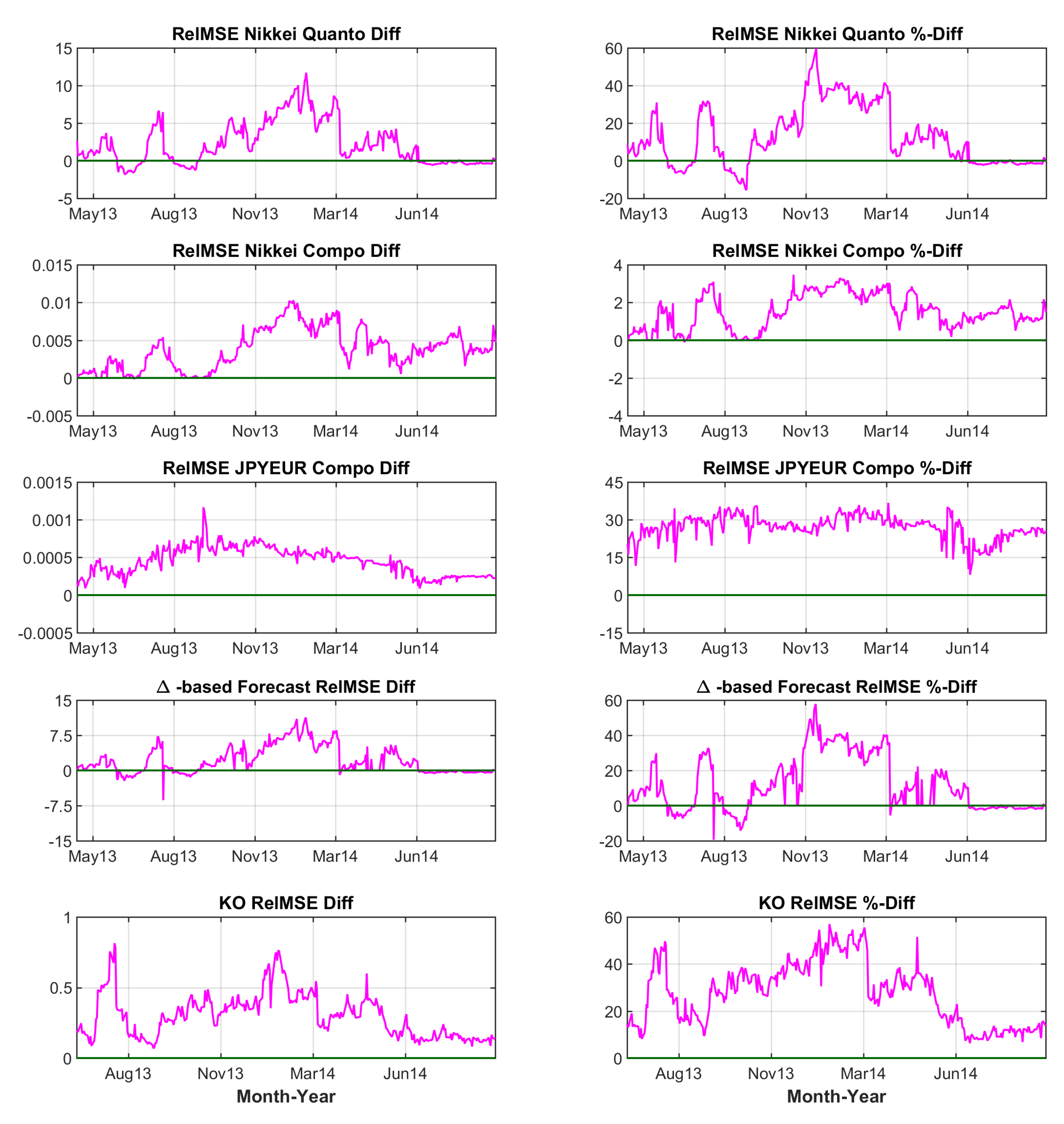
As the Black–Scholes model is contained in the NTS framework, RelMSE differences are non-negative and positive values support the NTS model. While on some days both models seem to fit equally well, the NTS setup generally outperforms.
(2)
Although parameter stability seems to be an issue for the NTS model, the use of yesterday’s parameter values still produces more realistic model prices than the Black–Scholes setup. This is of practical relevance as traders have to resort to readily available parameter values.
(3)
Concerning barrier risk, the NTS model clearly dominates the Gaussian version. The main reason for this follows from Figure 2. To accommodate fat tails, the Gaussian setup generally produces distributions that are flatter in the center. However, when the barriers of KO warrants are close enough to the current underlying level, significant overestimation of knock-out risk and, thus, lower prices will result. Moreover, we may – in some heuristic sense – relate our findings to hedging strategies. Since perfect delta-hedging is impossible, due to the unremovable jump risk in the NTS setup16, we can expect prices to be higher.
To summarize our empirical findings the NTS model generally performs better than the classical Black–Scholes setup, although parameter instability might be a concern. We will address this issue in the next section.
A last remark about stability of our Monte-Carlo pricing scheme: Given the fact that we work with M = 20 , 000 sample paths, one might raise concerns about potential noise in our simulation-based KO prices. However, as discussed before, the payoff of the considered barrier options is just binary—either an investor gets paid 0 EUR or 10 EUR, depending on whether the barriers have been touched/violated or not. In particular, the final level of the Nikkei 225 does play no role. Therefore one might already presume that not too many paths are necessary for stable simulation results. Figure 8 further substantiates this presumption.

5. Compo Options and a New Calibration Algorithm

As discussed in the previous section, given real market prices, the Black–Scholes as well as the NTS setup are not uniquely identified when using only quanto pricing formulas to calibrate risk neutral parameters. For the Black–Scholes model, this can be seen directly from Equation (1), since
σ X 2 2 ρ σ X σ Y + σ Y 2 = A and σ Y 2 ρ σ X σ Y = B ,
do not give rise to a unique solution given A and B. The same is true for the NTS assumption as it contains the Black–Scholes model. This problem is also well-known for other Lévy-based market setups and has led to stepwise calibration algorithms (see, for example, Guillaume (2013)) or the reduction of the given parameter space by combining historical estimation and classical calibration (cf. Guillaume and Schoutens (2012) about a similar discussion for the Heston stochastic volatility model).
To overcome this problem, quanto option practitioners frequently calibrate the Gaussian model via compo options. Based on the market setup in Assumption 1, the implied FX volatility, σ Y , can be identified by just using FX options. For compo equity derivatives, however, the correlation, ρ , and the implied equity volatility, σ X , come into play leading to a similar identification issue as with just using quanto options. As, for example, Ballotta et al. (2015) point out, traders usually set ρ to the historical market correlation and then calibrate σ Y and σ X . This has the additional charm that one can adjust ρ for quanto options to reflect the fact that these derivatives are typically more difficult to hedge. In fact, Ballotta et al. (2015) show that there are significant differences between the historical and the quanto implied correlations. Therefore, for the Gaussian case we adopt the following calibration algorithm:
Algorithm BS
Step 1: 
Calibrate σ Y via compo options on 1 / F .
Step 2: 
Take the historical correlation ρ = 0.2216 (based on the roughly 12-year sample in Section 2) and calibrate σ X via compo options on N.
Step 3: 
Use the implied volatilities σ X and σ Y obtained in Step 2 and calibrate ρ via quanto options on N.
Note that this procedure can be compared to that in Brigo and Alfonsi (2005) who calibrated interest and credit rates separately, as they showed that the correlation impact on theoretical CDS prices is fairly small. Our argument here is somewhat different, but leads to a comparably simple and straightforward calibration algorithm. From a theoretical perspective, we need to extend the presented pricing formulas to compo options. Even though this is a straightforward calculation, we are not aware of the relevant Black–Scholes formula in the rather scarce quanto pricing literature.
Therefore, we establish and prove the pricing formula, which also leads to a better understanding of the mathematical difficulties arising for the NTS model.17
Theorem 3.
Given Assumption 1 and Theorem 1 with T > 0 , the prices C t N , compo ( K , T ) and C t F , compo ( K , T ) of European compo call options on N ( T ) and 1 / F ( T ) with strike K > 0 at time 0 t < T can be calculated via
C t N , compo ( K , T ) = exp { r d ( T t ) } E Q [ F ( T ) ( N ( T ) K ) + | F t ] = 1 2 π R V ( t ) Φ ( d 1 [ η ] ) K F ( t ) e r f ( T t ) Φ ( d 2 [ η ] ) e 1 2 η 2 d η , σ Y ρ σ X V ( t ) Φ ( d 1 0 ) K F ( t ) e r f ( T t ) Φ ( d 2 0 ) , σ Y ρ = σ X
where
d 1 [ η ] = log V ( t ) K F ( t ) + ( r f + 1 2 [ σ X 2 + σ Y 2 2 σ X σ Y ρ ] ) ( T t ) | σ Y ρ σ X | T t 1 ρ 2 | ρ σ X / σ Y | η , d 2 [ η ] = d 1 [ η ] | σ Y ρ σ X | + σ Y ( 1 ρ 2 ) | ρ σ X / σ Y | T t
and
d 1 0 = log V ( t ) K F ( t ) + ( r f 1 2 [ σ X 2 σ Y 2 ] ) ( T t ) σ Y 1 ρ 2 T t , d 2 0 = d 1 0 σ Y 1 ρ 2 T t .
Furthermore, we have
C t F , compo ( K , T ) = exp { r d ( T t ) } E Q 1 F ( T ) K 1 F ( T ) + F t = Φ ( d 2 ) e r d ( T t ) e r f ( T t ) Φ ( d 1 ) K F ( t )
where
d 1 = log ( K F ( t ) ) + r d r f + σ Y 2 2 ( T t ) σ Y T t , d 2 = d 1 σ Y T t .
To date, we only derived prices for compo FX calls. As detailed in Section 3, our data set also includes puts of that type. However, by invoking the model-free compo FX call-put-parity
P t F , compo ( K , T ) = exp { r f ( T t ) } K F ( t ) exp { r d ( T t ) } + C t F , compo ( K , T )
we can directly specify the necessary put prices.
Figure 9 summarizes the Black–Scholes parameters obtained by the stepwise calibration algorithm. Note that for equity compo options the historical correlation of 0.2216 is used. As discussed already in Section 2, this positive correlation implies a negative correlation between the Nikkei 225 in JPY and the JPYEUR exchange rate. In Step 3 of the above calibration algorithm, the correlation is adjusted on each day to optimize the fit for Nikkei 225 quanto options. Keeping in mind that we need (4) to interpret this quanto implied correlation, we realize that even though ρ seems to be lower in absolute terms, on most days the implied relationship between the Nikkei 225 in JPY and the JPYEUR rate is even more negative, i.e., stronger.
Furthermore, having calibrated ρ in Step 3, we examine how its value affects the fit of the compo options. The RelMSEs are compared in the bottom left graph in Figure 9. It turns out that the optimal parameters for quanto substantially differ from those for the compo options. This shows that the Black–Scholes model is not able to adequately capture the increased risk contained in quanto derivatives. Therefore, one could argue that the fitted ρ values reflect a charge for this additional risk and, thus, we will refer to quanto-adjusted parameters as quanto charge.
For the NTS model the situation is somewhat more delicate as, especially, the tail and tempering parameters, α and θ , affect both option types. In addition, as shown in Section 4, the implied values for these two parameters proved to be quite instable over time. A potential solution to this problem follows from Theorem 2. The chosen risk-neutral measure is obtained by just modifying the drift of the two-dimensional Brownian motion and leaving the tempered stable subordinator untouched. In other words, α and θ do not change under the measure change from P to Q .
As we are mainly interested in obtaining stable NTS parameters for quanto option pricing, we propose the following algorithm for the NTS framework:
Algorithm NTS
Step 1: 
Estimate α and θ using the bivariate log return history of V and F from Section 2.
Step 2: 
Calibrate the Y-parameters via compo options on 1 / F .
Step 3: 
Calibrate the X-parameters and the correlation ρ via compo options on N.
Step 4: 
Calibrate the quanto option formula using the Y-parameters obtained in Step 2, but let the X-parameters and the correlation, ρ , vary under the restriction that the relative Nikkei compo fit is not worse than that of the Black–Scholes model (see Algorithm BS).
To apply the algorithm, we need to establish the relevant compo formulas for the NTS model. At the start of the calibration procedure, α and θ are already fixed. To speed up computation, it helps to separate these two parameters from the others.
Theorem 4.
Given Assumption 2 and Theorem 2 with T > 0 , then the prices C t N , compo ( K , T ) and C t F , compo ( K , T ) of European compo call options on N ( T ) and F ( T ) with strike K > 0 at time 0 t < T can be calculated via
C t N , compo ( K , T ) = exp { r d ( T t ) } E Q [ F ( T ) ( N ( T ) K ) + | F t ] = 1 2 π R + [ A T t ( ζ ) K B T t ( ζ ) ] f T ( T t ) ( ζ ) d ζ ,
where, for ζ > 0 ,
f T ( T t ) ( ζ ) = 1 2 π R e i u ζ exp 2 [ T t ] θ 1 α 2 α ( θ i u ) α 2 θ α 2 d u
and
A T t ( ζ ) = V ( t ) e [ w X ( λ X 🟉 ) β X ] ( T t ) R e [ β X + λ X 🟉 + σ X 2 2 ( 1 ρ 2 ) ] ζ + ρ σ X ζ η Φ ( d 1 [ η , ζ ] ) e 1 2 η 2 d η ,
B T t ( ζ ) = F ( t ) e ( r f w Y ( λ Y 🟉 ) β Y ) ( T t ) R e [ β Y + λ Y 🟉 ] ζ + σ Y ζ η Φ ( d 2 [ η , ζ ] ) e 1 2 η 2 d η
with
d 1 [ η , ζ ] = d 2 [ η , ζ ] + σ X 1 ρ 2 ζ d 2 [ η , ζ ] = log V ( t ) K F ( t ) + [ r f + w Y ( λ Y 🟉 ) w X ( λ X 🟉 ) + β Y β X ] ( T t ) + ( β X + λ X 🟉 β Y λ Y 🟉 ) ζ σ X 1 ρ 2 ζ ( σ Y ρ σ X ) σ X 1 ρ 2 η .
For the compo FX call we have
C t F , compo ( K , T ) = exp { r d ( T t ) } E Q 1 F ( T ) K 1 F ( T ) + F t = R + [ e r d ( T t ) Φ ( d 2 [ ζ ] ) K D T t ( ζ ) ] f T ( T t ) ( ζ ) d ζ
with
D T t ( ζ ) = F ( t ) e ( r f w Y ( λ Y 🟉 ) β Y ) ( T t ) exp [ β Y + λ Y 🟉 + σ Y 2 2 ] ζ Φ ( d 1 [ ζ ] )
where
d 1 [ ζ ] = log ( K F ( t ) ) + r d r f w Y ( λ Y 🟉 ) β Y ( T t ) + ( β Y + λ Y 🟉 + σ Y 2 ) ζ σ Y ζ , d 2 [ ζ ] = d 1 [ ζ ] σ Y ζ .
The following new representation for the pricing formula in Theorem 2 also helps to speed up Step 4 of the new calibration algorithm: As we do not need to minimize over α and θ , we can calculate upfront the subordinator density on a chosen grid and, thus, improve significantly on the otherwise supreme Fast Fourier Transform Algorithm.
Theorem 5.
Given Assumption 2 and Theorem 2 with T > 0 , assume σ X 2 + σ Y 2 2 ρ σ X σ Y > 0 . Then, for K > 0 , F f i x > 0 and 0 t < T , we have
C t q u a n t o ( K , T ) = exp { r d ( T t ) } E Q [ F f i x ( N ( T ) K ) + | F t ] = R + [ E T t ( ζ ) K e r d ( T t ) Φ ( d 2 [ ζ ] ) ] f T ( T t ) ( ζ ) d ζ
where for ζ > 0
f T ( T t ) ( ζ ) = ( 2 π ) 1 R e i u ζ exp 2 [ T t ] θ 1 α 2 α ( θ i u ) α 2 θ α 2 d u , E T t ( ζ ) = N ( t ) e [ r d + r f + w Y ( λ Y 🟉 ) + β Y w X ( λ X 🟉 ) β X ] ( T t ) × exp [ β X + λ X 🟉 β Y λ Y 🟉 + 1 2 ( σ X 2 + σ Y 2 2 ρ σ X σ Y ) ] ζ Φ ( d 1 [ ζ ] )
with
d 1 [ ζ ] = d 2 [ ζ ] + σ X 2 + σ Y 2 2 ρ σ X σ Y ζ , d 2 [ ζ ] = log N ( t ) K + r f + w Y ( λ Y 🟉 ) w X ( λ X 🟉 ) + β Y β X ( T t ) + ( β X + λ X 🟉 β Y λ Y 🟉 ) ζ σ X 2 + σ Y 2 2 ρ σ X σ Y ζ
The empirical results obtained for the NTS model are illustrated in Figure 10. One of our main findings is that when fixing α and θ upfront and including compo options, the calibrated parameters (especially drift and skewness) are much more stable over time than when just considering quanto options, as was done in Section 4. Even though some quanto implied parameters (i.e., quanto charges) are quite different from those coming from the Nikkei compo options, the two RelMSEs (bottom left) do not differ as much as in the Black–Scholes setting. This is in line with our earlier findings on the KO option fit in Section 4: The NTS model generally seems to be coping much better with the additional quanto risk. This is especially evident in the period November 2013 to March 2014.
Finally, as in Section 4, we use the calibrated parameters to calculated delta-based forecasts for the quanto options and compare the out-of-sample model fit for our double-barrier option data. The daily RelMSE differences (including those for the calibration fit) are shown in Figure 11.
Having α and θ fixed at the chosen values, the two models clearly differ and, therefore, it is not surprising that, on some days, the quanto fit of the Black–Scholes setup can be better. This can be seen especially for the last months of the sample period, where Figure 6 implied α -values close to 2. However, when considering the complete sample period, the NTS setup clearly dominates the Gaussian model for quanto and, especially, for FX compo options. Interestingly, even though the Nikkei compo fit is nearly the same (second row of Figure 11), the additional quanto charge is lower for the NTS model.
Furthermore, when looking at the delta-based forecasts for quanto options, the NTS setup implies more stable parameters over time than the Black–Scholes model.
Finally, for the double-barrier options, the NTS framework clearly outperforms the Black–Scholes setup again even though its advantage is lower than in Section 4. However this can be explained by the fact that the additional compo options make it harder for every model.

6. Conclusions

Conducting an extensive empirical study of daily data on quanto retail options we have compared the adequacy of a classical Black–Scholes-type framework and the newly proposed NTS model of Kim et al. (2015). However, direct calibration led to problems with identification and parameter instability. This was overcame by a stepwise procedure making use of compo options and combining historical estimation and calibration. Our results indicate that the non-Gaussian NTS model, a member of the general Lévy class, does not only provide a better in-sample-fit for observed quanto options prices. It also provides better forecasts for model parameters as well as out-of-sample accuracy when pricing exotic double-barrier options.
Given that the stepwise calibration procedure employed in Section 5 favors in some time periods (e.g. June–September 2014) the Black–Scholes (i.e., α = 2 ) over the NTS setup (i.e., α < 2 ), a time-varying parameter approach, which allows α (and possibly other parameters) to change over time, might be a promising extension of our analysis.

Author Contributions

All authors contributed equally to the paper. All authors have read and agreed to the published version of the manuscript.

Funding

This research received no external funding.

Institutional Review Board Statement

Not applicable.

Informed Consent Statement

Not applicable.

Data Availability Statement

Our used data was obtained from publicly available sources as described in Section 3 and Appendix B.

Conflicts of Interest

The authors declare no conflict of interest.

Appendix A. Proofs

Proof of Theorem 3.
We start with the quanto equity option. Assume σ Y ρ > σ X and decompose
C t N , compo ( K , T ) = exp { r d ( T t ) } E Q [ F ( T ) ( N ( T ) K ) + | F t ] = exp { r d ( T t ) } E Q [ ( V ( T ) K F ( T ) ) + | F t ] = exp { r d ( T t ) } E Q [ 1 { V ( T ) K F ( T ) } V ( T ) | F t ] : = ( I ) K E Q [ 1 { V ( T ) K F ( T ) } F ( T ) | F t ] : = ( I I )
Setting
d 1 🟉 = log V ( t ) K F ( t ) + ( r f 1 2 [ σ X 2 σ Y 2 ] ) ( T t ) σ Y 1 ρ 2 ] [ B ¯ Y ( T ) B ¯ Y ( t ) ] ( σ Y ρ σ X ) T t ,
the first term becomes
( I ) = V ( t ) E Q E Q 1 { V ( T ) K F ( T ) } V ( T ) V ( t ) | F t F B ¯ Y | F t = V ( t ) E Q ( 2 π ) 1 / 2 d 1 🟉 e r d ( T t ) σ X 2 2 ( T t ) + σ X T t ξ e 1 2 ξ 2 d ξ | F t = V ( t ) e r d ( T t ) E Q ( 2 π ) 1 / 2 d 1 🟉 e 1 2 [ ξ σ X T t ] 2 d ξ | F t = V ( t ) e r d ( T t ) E Q ( 2 π ) 1 / 2 d 1 🟉 σ X T t e 1 2 η 2 d η | F t = V ( t ) e r d ( T t ) E Q Φ ( d 1 🟉 σ X T t ) | F t = V ( t ) e r d ( T t ) ( 2 π ) 1 / 2 R Φ ( d 1 [ η ] ) e 1 2 η 2 d η
with d 1 [ η ] as in the assertion. By similar arguments, the second simplifies to
( I I ) = F ( t ) E Q E Q 1 { V ( T ) K F ( T ) } F ( T ) F ( t ) | F t F B ¯ Y | F t = F ( t ) e r d r f + σ Y 2 2 ( ρ 2 1 ) ( T t ) E Q e σ y 1 ρ 2 [ B ¯ Y ( T ) B ¯ Y ( t ) ] Φ ( d 1 🟉 σ Y ρ T t ) | F t = F ( t ) e r d r f + σ Y 2 2 ( ρ 2 1 ) ( T t ) 1 2 π R e σ y ( 1 ρ 2 ) ( T t ) η Φ ( d 1 [ η ] ( σ Y ρ σ X ) T t ) ) e 1 2 η 2 d η = F ( t ) e ( r d r f ) ( T t ) 1 2 π R Φ ( d 2 [ ξ ] ) e 1 2 ξ 2 d ξ
with d 2 [ ξ ] as specified by the theorem. Combining ( I ) and ( I I ) , we obtain the stated formula. The cases σ Y ρ < σ X and σ Y ρ = σ X can be derived via similar calculations. It remains to show the formula for the compo FX option. With d 1 and d 2 as stated in the theorem, this will be done by rewriting the compo call option as K quanto put options via
C t F , compo ( K , T ) = e r d ( T t ) E Q 1 F ( T ) K 1 F ( T ) + F t = e r d ( T t ) K E Q [ ( K 1 F ( T ) ) + | F t ] = e r f ( T t ) ( r d r f ) ( T t ) K E Q [ ( K 1 F ( T ) ) + | F t ] = Φ ( d 2 ) e r d ( T t ) e r f ( T t ) Φ ( d 1 ) K F ( t ) .
Proof of Theorem 4.
Again we start with the compo equity option. With T being independent of ( B X , B Y ) , we can condition on the subordinator and proceed as in the proof of Theorem 3:
C t N , compo ( K , T ) = e r d ( T t ) E Q [ F ( T ) ( N ( T ) K ) + | F t ] = e r d ( T t ) E Q [ E Q [ ( V ( T ) K F ( T ) ) + | F t F T ] | F t ] = e r d ( T t ) E Q E Q [ 1 { V ( T ) K F ( T ) } V ( T ) | F t F T ] : = ( I ) K E Q [ 1 { V ( T ) K F ( T ) } F ( T ) | F t F T ] : = ( I I ) | F t .
In contrast to the Black–Scholes-type model, ( B X , B Y ) is correlated without assuming partly equal sample paths. However, using the well-known fact that conditional Gaussian random variables are again normally distributed, we obtai, n for 0 t < T ,
B X ( T ( T ) ) B X ( T ( t ) ) | B Y ( T ( T ) ) B Y ( T ( t ) ) , F T
N ρ [ B Y ( T ( T ) ) B Y ( T ( t ) ) ] , [ T ( T ) T ( t ) ] ( 1 ρ 2 ) .
Since T ( T ) T ( t ) 0 a.s., we set
d 2 🟉 = log V ( t ) K F ( t ) + [ r f + w Y ( λ Y 🟉 ) w X ( λ X 🟉 ) + β Y β X ] ( T t ) + ( β X + λ X 🟉 β Y λ Y 🟉 ) [ T ( T ) T ( t ) ] σ X 1 ρ 2 T ( T ) T ( t ) ( σ Y ρ σ X ) [ B Y ( T ( T ) ) B Y ( T ( t ) ) ] σ X 1 ρ 2 T ( T ) T ( t )
Now we can proceed with the individual terms, starting with
( I ) = V ( t ) E Q E Q 1 { V ( T ) K F ( T ) } V ( T ) V ( t ) | F t σ ( B Y ( T ( T ) ) B Y ( T ( t ) ) ) F T | F t F T = V ( t ) E Q [ 1 2 π d 2 🟉 exp [ r d w X ( λ X 🟉 ) β X ] ( T t ) + ( β X + λ X 🟉 ) [ T ( T ) T ( t ) ] × exp ρ σ X [ B Y ( T ( T ) ) B Y ( T ( t ) ) ] + σ X T ( T ) T ( t ) 1 ρ 2 ξ e 1 2 ξ 2 d ξ | F t F T ] = V ( t ) e [ r d w X ( λ X 🟉 ) β X ] ( T t ) × E Q [ exp [ β X + λ X 🟉 + σ X 2 2 ( 1 ρ 2 ) ] [ T ( T ) T ( t ) ] + ρ σ X [ B Y ( T ( T ) ) B Y ( T ( t ) ) ] × 1 2 π d 2 🟉 exp 1 2 [ ξ σ X T ( T ) T ( t ) 1 ρ 2 ] 2 d ξ | F t F T ] = V ( t ) e [ r d w X ( λ X 🟉 ) β X ] ( T t ) × E Q [ exp [ β X + λ X 🟉 + σ X 2 2 ( 1 ρ 2 ) ] [ T ( T ) T ( t ) ] + ρ σ X [ B Y ( T ( T ) ) B Y ( T ( t ) ) ] × Φ ( d 2 🟉 + σ X T ( T ) T ( t ) 1 ρ 2 ) | F t F T ] = 1 2 π V ( t ) e [ r d w X ( λ X 🟉 ) β X ] ( T t ) × R exp [ β X + λ X 🟉 + σ X 2 2 ( 1 ρ 2 ) ] [ T ( T ) T ( t ) ] + ρ σ X T ( T ) T ( t ) η × Φ ( d 2 🟉 + σ X T ( T ) T ( t ) 1 ρ 2 ) e 1 2 η 2 d η
Moreover, we have
( I I ) = F ( t ) E Q E Q 1 { V ( T ) K F ( T ) } F ( T ) F ( t ) | F t σ ( B Y ( T ( T ) ) B Y ( T ( t ) ) ) F T | F t F T = F ( t ) e ( r d r f w Y ( λ Y 🟉 ) β Y ) ( T t ) × E Q exp ( β Y + λ Y 🟉 ) [ T ( T ) T ( t ) ] + σ Y [ B Y ( T ( T ) ) B Y ( T ( t ) ) ] Φ ( d 2 🟉 ) | F t F T = 1 2 π F ( t ) e ( r d r f w Y ( λ Y 🟉 ) β Y ) ( T t ) × R exp ( β Y + λ Y 🟉 ) [ T ( T ) T ( t ) ] + σ Y T ( T ) T ( t ) η Φ ( d 2 🟉 ) e 1 2 η 2 d η
Combining everything, we obtain the assertion. The formula for the compo FX call can be derived via similar, but rather tedious, calculations. □
Proof of Theorem 5.
The proof follows along the lines of Theorem 4 and involves, again, a tedious calculation. □

Appendix B. Identifier Numbers (WKNs) of All RSPs Used in Empirical Analysis

Nikkei 225 open-end-tracker: 252140, 698516, 702976, 787332, CB5UYN, HV1NKY, DR1CD5, DZ2NX7, DZ2RZC
Nikkei 225 quanto call options: SG3424, SG3425, SG3426, SG3427, SG3428, SG3429, SG343A, SG343B, SG343C, SG343D, SG343E, SG343F, SG343G, SG343H, SG343J, SG343K, SG343L, SG343M, SG343N, SG343P, SG343Q, SG343R, SG343S, SG343T, SG343U, SG343V, SG343W, SG343X, SG343Y
Nikkei 225 compo call options: SG196L, SG196M, SG3WBJ, SG3WBK, SG3WBL, SG3WBM, SG3WBP, SG3WBQ, SG3WBR, SG3WBS, SG3WBT, SG3WBU, SG3WBV, SG2L0T, SG2L0U, SG2L0V, SG2L0W, SG2WQW, SG2WQX, SG2WQY
EURJPY compo options: SG3W6J, SG3W6K, SG3W6L, SG3W6M, SG3W6N, SG3W6P, SG3W6Q, SG3W6R, SG3W6S, SG3W6T, SG3W6U, SG3W6V, SG3W6W, SG3W6X, SG3W6Y, SG3W6Z, SG3W60, SG3W61
Nikkei 225 KO options: SG36ET, SG36EV, SG36EY, SG36EZ, SG36E0, SG36E1, SG36E4, SG4EFS, SG4EFT, SG4EFU, SG4EFV, SG4EFW, SG4EFX, SG4EFY, SG4EFZ, SG4EF0, SG4EF1, SG4EF2, SG4EF3, SG4EF4, SG4EF5, SG4EF6, SG4EF7, SG4EF8, SG4EF9, SG4EGA, SG4EGB, SG4EGC, SG4EGD, SG4EGE, SG4EGF, SG4EGG, SG4EGH, SG4EGJ, SG4EGK, SG4EGL, SG4EGM, SG4EGN, SG4EGP, SG4EGQ, SG4EGR, SG4EGS, SG4EGT, SG4EGU, SG4EGV, SG4EGW, SG4EGX, SG4EGY, SG4FZL, SG4FZM, SG4FZN, SG4FZP, SG4FZQ, SG4FZT, SG4FZU, SG4FZV, SG4FZW, SG4FZX, SG4FZZ, SG4FZ0, SG4FZ1, SG4FZ2, SG4FZ3, SG4FZ4, SG4FZ5, SG4FZ6, SG4FZ7, SG4FZ8, SG4FZ9, SG4F0A, SG4F0B, SG4F0C, SG4F0D, SG4F0E, SG4F0F, SG4NCZ, SG4NC0, SG4NC1, SG4NC2, SG4NC3, SG4NC4, SG4NC5, SG4NC6, SG4NC7, SG4NC8, SG4NC9, SG4NDA, SG4NDB, SG4NDC, SG4NDD, SG4S20, SG4S21, SG4S22, SG4S23, SG4S24, SG4S25, SG4S26, SG4S27, SG4S28, SG4S29, SG4S3A, SG4S3B, SG4S3C, SG4S3D, SG4S3E, SG4S3F, SG4S3G, SG4S3H, SG4S3J, SG4S3K, SG4S3L, SG4S3M, SG4S3N, SG4S3P, SG4S3Q, SG4S3R, SG4S3S, SG4S3T, SG4S3U, SG4S3V, SG4S3W, SG4S3X, SG4S3Y, SG4S3Z, SG4S30, SG41DF, SG41DG, SG41DH, SG41DJ, SG41DK, SG41DL, SG41DM, SG41DN, SG41DP, SG41DQ, SG41DR, SG41DS, SG41DT, SG42UV, SG42UW, SG42UX, SG42UY, SG42UZ, SG42U0, SG42U1, SG42U2, SG42U3, SG42U4, SG42U5, SG42U6, SG42U7, SG42U8, SG42U9, SG42VA, SG42VB, SG42VC, SG42VD, SG42VE, SG42VF, SG42VG, SG42VH, SG42VJ, SG42VK, SG42VL, SG42VM, SG42VN, SG42VP, SG4739, SG474A, SG474B, SG474C, SG474D, SG474E, SG474F, SG474G, SG474H, SG474J, SG474K, SG474L, SG474M, SG474N, SG474P, SG474Q, SG474R, SG474S, SG474T, SG474U, SG474V, SG474L, SG474X, SG474Y, SG474Z, SG4740, SG4741, SG4742, SG4743, SG4744, SG4745, SG4746, SG4747, SG4748, SG4749, SG475A, SG475B, SG475C, SG475D, SG475E, SG475F, SG475G, SG475H, SG475J, SG475K, SG475L, SG475M, SG475N, SG475P, SG475Q, SG475R, SG475S, SG475T, SG475U, SG475V, SG475W, SG475X, SG475Y, SG475Z, SG4750, SG4751, SG4752, SG4753, SG4754, SG4755, SG4756, SG5BFZ, SG5BF0, SG5BF1, SG5BF2, SG5BF3, SG5BF4, SG5BF5, SG5BF6, SG5BF7, SG5BF8, SG5BF9, SG5BGA, SG5BGB, SG5BGC, SG5BGD, SG5LUU, SG5LUV, SG5LUW, SG5LUX, SG5LUY, SG5LUZ, SG5LU0, SG5LU1, SG5LU2, SG5LU3, SG5LU4, SG5LU5, SG5LU6, SG5LU7, SG5LU8, SG5LU9, SG5LVA, SG5LVB, SG5LVC, SG5LVD, SG5LVE, SG5LVF, SG5LVG, SG5LVH, SG5LVJ, SG5LVK, SG5LVL, SG5LVM, SG5LVN, SG5LVP, SG5LVQ, SG5LVR, SG5LVS, SG5LVT, SG5LVU, SG5LVV, SG5NVU, SG5NVV, SG5NVW, SG5NVX, SG5NVY, SG5NVZ, SG5NV0, SG5NV1, SG5NV2, SG5NV3, SG5NV4, SG5NV5, SG5NV6, SG5NV7, SG5NV8, SG5NV9, SG5NWA, SG5NWB, SG5NWC, SG5NWD, SG5NWE, SG5NWF, SG5NWG, SG5NWH, SG5NWJ, SG5NWK, SG5NWL, SG5NWM, SG5QKA, SG5QKB, SG5QKC, SG5QKD, SG5QKE, SG5QKF, SG5QKG, SG5QKH, SG5QKJ, SG5QKK, SG5QKL, SG5QKM, SG5QKN, SG5QKP, SG5QKQ, SG5QKR, SG5QKS, SG5QKT, SG5QKU, SG5QKV, SG5QKW, SG5QKX, SG5QKY, SG5QKZ, SG5QK0, SG5QK1, SG5QN3, SG5QN4, SG5VQL, SG5VQM, SG5VQN, SG5VQP, SG5VQQ, SG5VQR, SG5VQS, SG5VQT, SG5VQU, SG5VQV, SG5VQW, SG5VQX, SG5VQY, SG5VQZ, SG5VQ0, SG5VQ1, SG5VQ2, SG5V0G, SG5V0H, SG5V0J, SG5V0K, SG5V0L, SG5V0M

References

  1. Baeumer, Boris, and Mark M. Meerschaert. 2010. Tempered stable Lévy motion and transit super-diffusion. Journal of Computational and Applied Mathematics 233: 2438–48. [Google Scholar] [CrossRef] [Green Version]
  2. Ballotta, Laura, Griselda Deelstra, and Grégory Rayée. 2015. Quanto Implied Correlation in a Multi-Lévy Framework. Available online: http://papers.ssrn.com/sol3/papers.cfm?abstract_id=2569015 (accessed on 10 October 2020).
  3. Barndorff-Nielsen, Ole Eiler, and Sergei Z. Levendorskii. 2001. Feller processes of normal inverse Gaussian type. Quantitative Finance 1: 318–31. [Google Scholar] [CrossRef]
  4. Barndorff-Nielsen, Ole E., and Neil Shephard. 2001. Normal Modified Stable Processes. Department of Economics, Discussion Paper Series; Oxford: University of Oxford, p. 72. [Google Scholar]
  5. Baxter, Martin, and Andrew Rennie. 1996. Calculus: An Introduction to Derivative Pricing. Cambridge: Cambridge University Press. [Google Scholar]
  6. Bianchi, Michele L., Svetlozar R. Rachev, Young S. Kim, and Frank J. Fabozzi. 2010. Tempered stable distributions and processes in finance: Numerical analysis. In Mathematical and Statistical Methods for Actuarial Sciences and Finance. Edited by Marco Corazza and Claudio Pizzi. Berlin and Heidelberg: Springer. [Google Scholar]
  7. Branger, Nicole, and Matthias Muck. 2012. Keep on smiling? The pricing of Quanto options when all covariances are stochastic. Journal of Banking & Finance 36: 1577–91. [Google Scholar]
  8. Brigo, Damiano, and Aurélien Alfonsi. 2005. Credit default swap calibration and derivatives pricing with the SSRD stochastic intensity model. Finance and Stochastics 9: 29–42. [Google Scholar] [CrossRef]
  9. Broadie, Mark, and Paul Glasserman. 1997. A continuity correction for discrete barrier options. Mathematical Finance 7: 325–48. [Google Scholar] [CrossRef] [Green Version]
  10. Carr, Peter, and Dilip Madan. 1999. Option pricing and the Fast Fourier Transform. Journal of Computational Finance 2: 61–73. [Google Scholar] [CrossRef] [Green Version]
  11. Chen, Andrew H., and John W. Kensinger. 1990. An analysis of market-index certificates of deposit. Journal of Financial Services Research 4: 93–110. [Google Scholar] [CrossRef]
  12. Chen, Kuang C., and R. Stephen Sears. 1990. Pricing the SPIN. Financial Management 19: 36–47. [Google Scholar] [CrossRef]
  13. Delbaen, Freddy, and Walter Schachermayer. 1994. A general version of the fundamental theorem of asset pricing. Mathematische Annalen 312: 463–520. [Google Scholar] [CrossRef]
  14. Derman, Emanuel, Piotr Karasinski, and Jeffrey Wecker. 1990. Understanding guaranteed exchange-rate contracts in foreign stock investments. In Goldman Sachs Quantitative Strategies Research Notes. New York: Goldman Sachs. [Google Scholar]
  15. Dimitroff, Georgi, Alexander Szimayer, and Andreas Wagner. 2009. Quanto Option Pricing in the Parsimonious Heston Model. Available online: https://ssrn.com/abstract=1477387 (accessed on 23 September 2009).
  16. Eberlein, Ernst, and Kathrin Glau. 2014. Variational solutions of the pricing PIDEs for European options in Lévy models. Applied Mathematical Finance 21: 417–50. [Google Scholar] [CrossRef]
  17. Eberlein, Ernst, Kathrin Glau, and Antonis Papapantoleon. 2009. Analyticity of the Wiener-Hopf factors and valuation of exotic options in Lévy models. In Advanced Mathematical Methods for Finance. Berlin and Heidelberg: Springer, pp. 223–45. [Google Scholar]
  18. Eberlein, Ernst, Kathrin Glau, and Antonis Papapantoleon. 2010. Analysis of Fourier transform valuation formulas and applications. Applied Mathematical Finance 17: 211–40. [Google Scholar] [CrossRef] [Green Version]
  19. Eberlein, Ernst, and Ulrich Keller. 1995. Hyperbolic distributions in finance. Bernoulli 1: 281–99. [Google Scholar] [CrossRef]
  20. Eberlein, Ernst, Ulrich Keller, and Karsten Prause. 1998. New insights into smile, mispricing and value at risk: the hyperbolic model. Journal of Business 71: 371–405. [Google Scholar] [CrossRef] [Green Version]
  21. Eberlein, Ernst, Antonis Papapantoleon, and Albert N. Shiryaev. 2009. Esscher transform and the duality principle for multidimensional semimartingales. Annals of Applied Probability 19: 1944–71. [Google Scholar] [CrossRef]
  22. Escobar, Marcos, Peter Hieber, and Matthias Scherer. 2014. Efficiently pricing double barrier derivatives in stochastic volatility models. Review of Derivatives Research 17: 191–216. [Google Scholar] [CrossRef]
  23. Fink, Holger, Sebastian Geissel, Jörn Sass, and Frank T. Seifried. 2019. Implied risk aversion: an alternative rating system for retail structured products. Review of Derivatives Research 22: 357–87. [Google Scholar] [CrossRef]
  24. Geman, Hélyette, and Marc Yor. 1996. Pricing and hedging double-barrier options: a probabilistic approach. Mathematical Finance 6: 365–78. [Google Scholar] [CrossRef] [Green Version]
  25. Gerber, Hans. U., and Elias S. W. Shiu. 1994. Option pricing by Esscher transforms. Transactions of Society of Actuaries 48: 99–191. [Google Scholar]
  26. Guillaume, Florence. 2013. The αVG model for multivariate asset pricing: calibration and extension. Review of Derivatives Research 16: 25–52. [Google Scholar] [CrossRef]
  27. Guillaume, Florence, and Wim Schoutens. 2012. Calibration risk: Illustrating the impact of calibration risk under the Heston model. Review of Derivatives Research 15: 57–79. [Google Scholar] [CrossRef] [Green Version]
  28. Kawai, Reiichiro, and Hiroki Masuda. 2012. Infinite variation tempered stable Ornstein-Uhlenbeck processes with discrete observations. Communications in Statistics-Simulation and Computation 41: 125–39. [Google Scholar] [CrossRef] [Green Version]
  29. Kim, Young S., Rosella Giacometti, Svetlozar T. Rachev, Frank J. Fabozzi, and Domenico Mignacca. 2012. Measuring financial risk and portfolio optimization with a non-Gaussian multivariate model. Annals of Operations Research 201: 325–43. [Google Scholar] [CrossRef] [Green Version]
  30. Kim, Young S., Jaesung Lee, Stefan Mittnik, and Jiho Park. 2015. Quanto option pricing in the presence of fat tails and asymmetric dependence. Journal of Econometrics 187: 512–20. [Google Scholar] [CrossRef] [Green Version]
  31. Kunitomo, Naoto, and Masayuki Ikeda. 1992. Pricing options with curved boundaries. Mathematical Finance 2: 275–98. [Google Scholar] [CrossRef]
  32. Park, Jiho, Youngrok Lee, and Jaesung Lee. 2013. Pricing of quanto option under the Hull and White stochastic volatility model. Communications of the Korean Mathmatical Society 28: 615–33. [Google Scholar] [CrossRef] [Green Version]
  33. Sato, Ken-Iti. 1999. Lévy Processes and Infinitely Divisible Distributions. Cambridge: Cambridge University Press. [Google Scholar]
  34. Schoutens, Wim, and Geert Van Damme. 2011. The β-variance gamma model. Review of Derivatives Research 14: 263–82. [Google Scholar] [CrossRef]
  35. Stoimenov, Pavel A., and Sascha Wilkens. 2005. Are structured products ’fairly’ priced? An analysis of the german market for equity-linked instruments. Journal of Banking and Finance 29: 2971–93. [Google Scholar] [CrossRef]
  36. Teng, Long, Matthias Ehrhardt, and Michael Günther. 2015. The pricing of quanto options under dynamic correlation. Journal of Computational and Applied Mathematics 275: 304–10. [Google Scholar] [CrossRef]
  37. Wilkens, Sascha, Carsten Erner, and Klaus Röder. 2003. The pricing of structured products in germany. Journal of Derivatives 11: 55–69. [Google Scholar] [CrossRef]
  38. Wilmott, Paul. 2006. Paul Wilmott on Quantitative Finance. Hoboken: John Whiley & Sons, Ltd. [Google Scholar]
1
All proofs are given in Appendix A. Appendix B identifies all RSPs used in our empirical study.
2
To avoid confusion, we will state the specific asset or currency in question in parentheses.
3
See Theorems 33.1 and 33.2 in Sato (1999).
4
Our option data set starts on 16 April 2013, cf. Section 3.
5
As discussed below, for the maximization procedure we imposed the restrictions α 1 and θ [ 20 , 200 ] .
6
CME options on its Nikkei 225 USD futures being one of the few exceptions.
7
Note, we focus only on simple option types and ignore more complex structures, like bonus-, lookback- or rainbow-certificates, which are left for future research.
8
The data were obtained from the data provider ARIVA.DE AG which also supplies the Frankfurt retail exchange Börse Frankfurt Zertifikate AG.
9
The identifiers (WKNs) of these tracker and the above plain vanilla as well as KO options are provided in Appendix B.
10
The main input factor (apart from time to maturity and interest rates) that changes is the price of the underlying, hence the term delta-based due to the Black–Scholes Greek delta.
11
The minimization is carried out in MATLAB using the routine fmincon. For this procedure the pricing formulas from Section 2 are invoked.
12
A very good overview and description of the various techniques can be found in Eberlein et al. (2009, 2010), or Eberlein and Glau (2014) and references therein.
13
The latter rely on the so-called Wiener-Hopf factorization, providing approximations of the characteristic functions of the running minimum and maximum and have been successfully applied to variance-gamma-type Lévy models (see Schoutens and Van Damme (2011)).
14
It should be mentioned that, for tax purposes, even in the case of a knock-out these types of products usually still pay a fixed amount of 0.001 EUR. For the sake of simplicity, we ignore this feature.
15
For all considerations, riskless rates were taken to be the lending rates from the European Central Bank and the Bank of Japan, respectively, at each trading day of the observation period.
16
See the discussion in the concluding section in Kim et al. (2015)
17
This and all other proof are presented in Appendix A.
Figure 1. Top: Nikkei 225 in EUR (left) and its log returns (right). Bottom: JPYEUR levels (left) and log returns (right). Sample period 4 January 2000 to 15 April 2013.
Jrfm 14 00136 g001
Figure 2. Estimated densities and log-densities based on the estimates reported in Table 1.
Jrfm 14 00136 g002
Figure 3. Simulated NTS price paths of V / F for varying α and θ . Remaining parameters were held fixed (see Table 1).
Jrfm 14 00136 g003
Figure 4. Top: Société Générale’s compo EURJPY options call prices (left) and compo Nikkei 225 call prices together with the Nikkei 225 tracker prices (right). Bottom left: Société Générale’s quanto call prices and the Nikkei 225 tracker price. Bottom right: Société Générale’s KO option prices and the Nikkei 225 tracker price. Vanilla (compo & quanto) contracts covering the period 16 April 2013 to 15 September 2014, KO options 19 June 2013 to 15 September 2015.
Jrfm 14 00136 g004
Figure 5. Quanto Calls: daily calibrated Black–Scholes parameters and RelMSE. Sample period 16 April 2013 to 15 September 2014.
Jrfm 14 00136 g005
Figure 6. Quanto Calls: daily calibrated implied ( X , Y ) NTS parameters and RelMSE. Sample period 16 April 2013 to 15 September 2014.
Jrfm 14 00136 g006
Figure 7. Quanto calls and KO options. Top: RelMSE-difference for the calibration. Middle: RelMSE-difference of the delta-based forecasts. Both sample period 16 April 2013 to 15 September 2014. Bottom: RelMSE-difference using the respective calibrated parameters from 19 June 2013 to 15 September 2014. Calculations were based on 20,000 sample paths simulated on each considered trading day assuming 5 daily trading hours and sampling every 15 s. Positive values indicate better performance of the NTS model.
Jrfm 14 00136 g007
Figure 8. Visualisation of noise in our chosen Monte-Carlo pricing scheme for two barrier options with different barriers (11,250/16,500 vs. 8400/18,800) and time to maturity (178 days vs. 548 days) for various numbers M of sample paths. Even though for maturities farther in the future, the NTS model still seems to miss market prices, its supremacy on the Gaussian setup is evident. Additionally, this miss does not necessarily present model issues as it could also be interpreted as evidence that issuer margins are especially high for such long product lifetimes.
Jrfm 14 00136 g008
Figure 9. Quanto and compo options: daily calibrated Black–Scholes parameters and RelMSEs. Sample period 16 April 2013 to 15 September 2014.
Jrfm 14 00136 g009
Figure 10. Quanto and compo options: daily calibrated ( X , Y ) NTS parameters and RelMSEs. Sample period 16 April 2013 to 15 September 2014.
Jrfm 14 00136 g010
Figure 11. Quanto, compo and KO options. Top three: RelMSE-difference for the quanto Nikkei, compo Nikkei and JPYEUR options. Bottom two: RelMSE-difference of the delta-based forecasts of quanto Nikkei call prices and RelMSE-difference for KO options. Sample period for vanilla options 16 April 2013 to 15 September 2014, for KO options 19 June 2013 to 15 September 2014. Positive values indicate better performance of the NTS model.
Jrfm 14 00136 g011
Table 1. Parameter estimates and bootstrapped 95% confidence intervals (in brackets) using 1000 simulated paths of length 3206 (inline with our historical return data set). For all time series, both the log-likelihood values and the model-selection criteria AIC and BIC strongly favor the NTS over the Black–Scholes model.
Black–ScholesNTS
Parameters
α 2 1.2962 [ 1.0662 , 1.4484 ]
θ 74.6539 [ 47.1372 , 127.7335 ]
μ X 0.0426 [ 0.2401 , 0.1593 ] 0.0454 [ 0.1625 , 0.0732 ]
β X 0.3192 [ 0.5694 , 0.0824 ]
σ X 0.2434 [ 0.2341 , 0.2525 ] 0.2477 [ 0.2396 , 0.2559 ]
μ Y 0.0147 [ 0.1180 , 0.0910 ] 0.0165 [ 0.0784 , 0.0450 ]
β Y 0.2062 [ 0.0798 , 0.3403 ]
σ Y 0.1319 [ 0.1270 , 0.1368 ] 0.1280 [ 0.1237 , 0.1321 ]
ρ 0.2216 [ 0.1724 , 0.2722 ] 0.2342 [ 0.1935 , 0.2770 ]
Nikkei 225 in EUR
log-likelihood   8834   8962
AIC 17 , 664 17 , 914
BIC 17 , 652 17 , 884
JPYEUR
log-likelihood    10 , 800     11 , 020
AIC 21 , 596 22 , 030
BIC 21 , 584 22 , 000
Bivariate Model
log-likelihood    19 , 708     20 , 154
AIC 39 , 406 40 , 288
BIC 39 , 376 40 , 233
Publisher’s Note: MDPI stays neutral with regard to jurisdictional claims in published maps and institutional affiliations.

