Article

Crisis and the Role of Money in the Real and Financial Economies—An Innovative Approach to Monetary Stimulus

1
Enterprise & Business Development, University of Hertfordshire, Enterprise Hub, Hatfield, Hertfordshire AL10 9AB, UK
2
Department of Media and Communications, London School of Economics and Political Science, London WC2A 2AE, UK
3
Sardex S.p.A., Viale Sant’Ignazio 16, 09038 Serramanna, Italy
*
Author to whom correspondence should be addressed.
J. Risk Financial Manag. 2021, 14(3), 129; https://doi.org/10.3390/jrfm14030129
Submission received: 28 February 2021 / Revised: 11 March 2021 / Accepted: 16 March 2021 / Published: 20 March 2021
(This article belongs to the Special Issue Monetary Plurality and Crisis)

Abstract

:
‘Financial crisis’ is sometimes regarded as synonymous with ‘economic crisis’, but this is an oversimplification and risks missing the feedback loops between the financial and real economies. In this paper, the role of money is revisited in the context of distinguishing the real economy from the financial economy. A theoretical framework is developed to explain how endogenous (bank credit) and central bank exogenous (quantitative easing, QE) money creation feed into the real and financial economies. It looks at how the velocity of monetary circulation varies between the two economies and across asset types within the financial economy. Monetary transmission mechanisms are set into a framework that helps explain how QE stimulus risks combining asset price bubbles with poor growth in the real economy. The real economy transmission mechanism of ‘helicopter money’ is given context, enabling an assessment of the efficacy of both the QE and helicopter money policy routes. Finally, we present a new type of monetary transmission, ‘Smart Helicopter Money’, to deliver monetary stimulus to innovators, SMEs and high-growth firms via both complementary currencies and a modified form of QE in order to achieve proportionally greater impact on the real economy.

Graphical Abstract

1. Introduction

In this paper, we postulate that developed nations have an economic base consisting of two separate and distinct economies: the real economy of Main Street, focused on ‘value adding’, and the financial economy of Wall Street, focused upon the wealth management of existing assets. The narrative in the real economy is one of output, capital investment, innovation and productivity, whilst in the financial economy it is of increases in existing asset values and yield. Both real and financial economies depend upon money to function and grow. The disconnect between the economies, in 2021, is reminiscent of the 1929 one described by Galbraith (1961) in his seminal work on the Wall Street Crash. Starting from say 1970, there has been growing divergence largely as a consequence of financial market deregulation. Starting with the breakdown of the fixed-currency Bretton Woods world, through to the repeal of the Glass Steagall Act in 1999, financial regulation barriers have been dismantled and the financial Prometheus allowed to let rip.
Financial deregulation has been associated with the prevailing dominance of libertarian (Friedman 1962; Hayek 1960) thought in conventional economics. This has seen mainstream monetary theory revert to the classical Quantity Theory in the Fisher (1911) formulation, supplanting the ‘liquidity preference’ framework of Keynes (1936). By juxtaposition and partly in reaction to this trend, Modern Monetary Theorists (Juniper et al. 2014) have presented an alternative framework where they envisage a world of limitless potential for central banks to ‘monetary-fund’ government deficits. They argue this allows the state to balance economic activity by acting as the ‘employer of last resort’.1
By contrast, we believe that whilst in the main money is created endogenously, central bank money creation to fund governments is constrained by the interplay between external capital flows, exchange rate fluctuations, and overall price growth and financial stability. Further, following Werner (1997, 2012),2 we argue that the separation between the real and financial economies results in protracted capital misallocation, as flows of funds and created credit are focused into purchasing existing assets in the pursuit of stable savings returns from known predictable cashflows and anticipated capital gains in asset values. Concurrently, the real economy requires a higher flow of funds into capital investment to support entrepreneurial growth in innovators, SMEs, and high-growth firms (Schumpeter 1934). Over-allocation of capital into the financial economy slows real economy growth rates and misprices financial economy assets (artificially depressing savings yields). This mismatch, in turn, leads to financial crises as markets force adjustments between asset prices and the real economy cashflows that support them.
For us, a financial crisis is a “liquidity freeze” where assets can no longer be turned into cash at a value aligned to their long-term discounted potential cashflows. The moment is general rather than specific (Feldstein 1991), so needs to cover more than one investor or group of investors and more than one company or asset class. The onset of the crisis is a ‘Minsky Moment’ (Minsky 1989).
As asset values fall in the financial economy, there can be an associated economic crisis as real-economy actors rein back spending and lenders tighten lending criteria. Economic crises have some similarities to financial crises, as they can start when economic actors have incurred debt to a level that they cannot service (Minsky 1989). Economic crises are also synonymous with monetary instability (Friedman 1960). We draw upon, develop, and interweave these themes to arrive at a 21st Century, high-level understanding of the relationship between money, financial markets, and the real economy.
More specifically, our view of a crisis is a situation where ‘business as usual’ is broken. Restrictive assumptions such as ‘rational expectations’ (Lucas 1976; Muth 1961), representative rational agent modelling, probability theory, and stochastic modelling fail to support understanding as in a crisis we face the uncertainty described by Frank Knight (Knight 1921). Arguably, this is one of the key challenges that Keynes (1936) addressed in his General Theory. Our analysis seeks to understand how changes in the monetary mass within both the real and financial economies act as a key factor in financial resource allocation to support innovation and economic growth, with mismatches driving financial asset bubbles and thereby acting as a crucial driver in the onset of both financial and economic crises. However, although both real and financial economies are part of one system, the monetary disconnect between them has profound importance. Specifically, growth in the monetary mass in the financial economy does not automatically pass into the real economy, so central bank stimulus targeting the financial economy is likely to have little direct impact on the real economy, although stress and trouble in the financial economy routinely spells trouble for the real economy.
Whilst money is normally created endogenously, since 2009 there has been an additional central bank exogenous ‘quantitative easing’ (QE) creation stream. Our understanding of how these monetary mass changes interact with both the real and the financial economies is enabled by utilizing the quantity equation into our two-economy paradigm. This simple innovation allows us to shed light on the interplay of money with economic activity in the real economy whilst providing insights into the bubbles and instabilities in the financial economy, which in turn can generate real economy instability. Not only does the quantity of money matter, but how new money is transmitted into the economy is crucial as to whether it will promote real economy activity and growth, or if it will feed asset value increases in the financial economy. This framework helps us understand why money injected via central banks’ QE has, despite its magnitude since 2009, generally become stuck in the financial economy and largely failed to reach the real economy. We suggest this blockage is largely the result of a failure to understand the differing monetary dynamics in the real and financial economies and the monetary mediation failures between them.
We conclude by noting that in the financial economy exogenous money (QE) stabilizes (in crisis) by inflating asset market values but lacks appropriate market-facing transmission mechanisms to carry QE into the real economy. Such real-economy QE support, in the context of the slow growth rates since 2008 and current Covid-19 pandemic growth losses, is urgently required to (i) promote crisis recovery; (ii) enhance economic growth rates by freeing real-economy credit constraints; (iii) support long-term economic/social goals such as decarbonizing the productive economy and/or promoting regional productive investment; (iv) a combination of all of the above.
Rather than opting for Friedman’s helicopter money (Friedman 1969), which is focused at consumers and whose benefit can be reduced through leakages to imports and saving(s) transferred into the financial economy, we opt for a ‘smart helicopter money’ concept to target the supply side of the real economy, which existing mechanisms fail to reach. To realize this we propose three options for transmission mechanisms to directly connect QE monetary expansion to real-economy growth by addressing those credit-starved innovators and SMEs that form the bedrock of all developed and developing economies.
The next section presents a qualitative analysis of time-series data from a number of public and private monetary and economic sources to provide evidence of the disconnect between the real and financial economies. Section 3 develops the main argument of the paper by generalizing the quantity equation for the two economies separately and detailing the monetary flows between them. It then analyses the sources and utilization of the monetary mass in the real and financial economies, providing a framework to explain the occurrence of financial crashes as a source of economic crises. It ends with an analysis of why conventional responses to financial and economic crises such as QE and helicopter money are not effective, and offers three new monetary policy channels to heal the real economy. Section 4 provides a brief clarification of the main concepts used, and Section 5 offers some conclusions.

2. Results

In this section we discuss almost exclusively empirical data to show the divergence between the real and financial economies since 1970, to give a sense of the asset composition of the financial economy, and to show that QE is much less effective at reaching the real economy than we all would wish.

2.1. The Roots of Divergence

Figure 1 shows the increase in the size of the financial sector in the United States since 1945. It is striking that assets in the financial sector grew more rapidly following the move from the gold standard to dollarization in 1971, the liberalization of the 1980s, and the subsequent repeal of the Glass Steagall Act in 1999.
Figure 2 shows how the pure financial sector’s assets rose from 29% of overall US financial assets in 1946 to 40% in 2019. The real and financial economies are separated by a black dotted boundary. This growth in financial assets has been enabled by financial innovation and leverage that have been applied (increasingly from about 1980 to 2000) to an already increasing US$ monetary mass. The definition of this monetary mass itself has also evolved as more instruments have tended to adopt “money-like” characteristics. Of particular importance in the modern financial economy are ‘repo’ and ‘reverse repo’3 agreements that underpin short-term money market fund arrangements and to a large extent enable the modern financial system.
Understanding the monetary landscape is confused by differences between the definitions used by different central banks and multilateral institutions (for example the US Federal Reserve and the IMF). Following the IMF definition of ‘Extended Broad Money’ (see Table 6.2 p. 1996 in Cartas and Harutyunyan (2017)), we estimate US Extended Broad Money by combining M2 money with institutional zero-demand money (MZM) and government cash, and repos. Debt securities are excluded to avoid double-counting risks as many of these are already involved in the repo market. Figure 3 gives a weekly view of this growth.
Comparing the growth in the annual money supply to the growth of financial assets in the household, business, and government sectors, we observe apparently loosely correlated relationships in Figure 4 (US Federal Reserve System 2020a). Although a statistical correlation test gives an r 2 value of only 0.02, qualitatively the curves follow each other for most of the 1981–2019 period. The major exception is some lagging of broad monetary mass relative to asset values in the 2000s (this area would benefit from follow-on econometric analysis). As can be seen in this figure, the repeal of the Glass-Steagall Act in 1999 and significant leverage utilized by professional traders with access to market trading platforms have had important systemic implications on the lag structure between the real and monetary economies. This change has been seen by some as the final “hammer blow’’ to the post-1929 regulatory system (Crawford 2011).

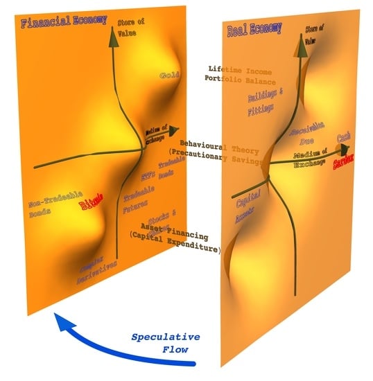
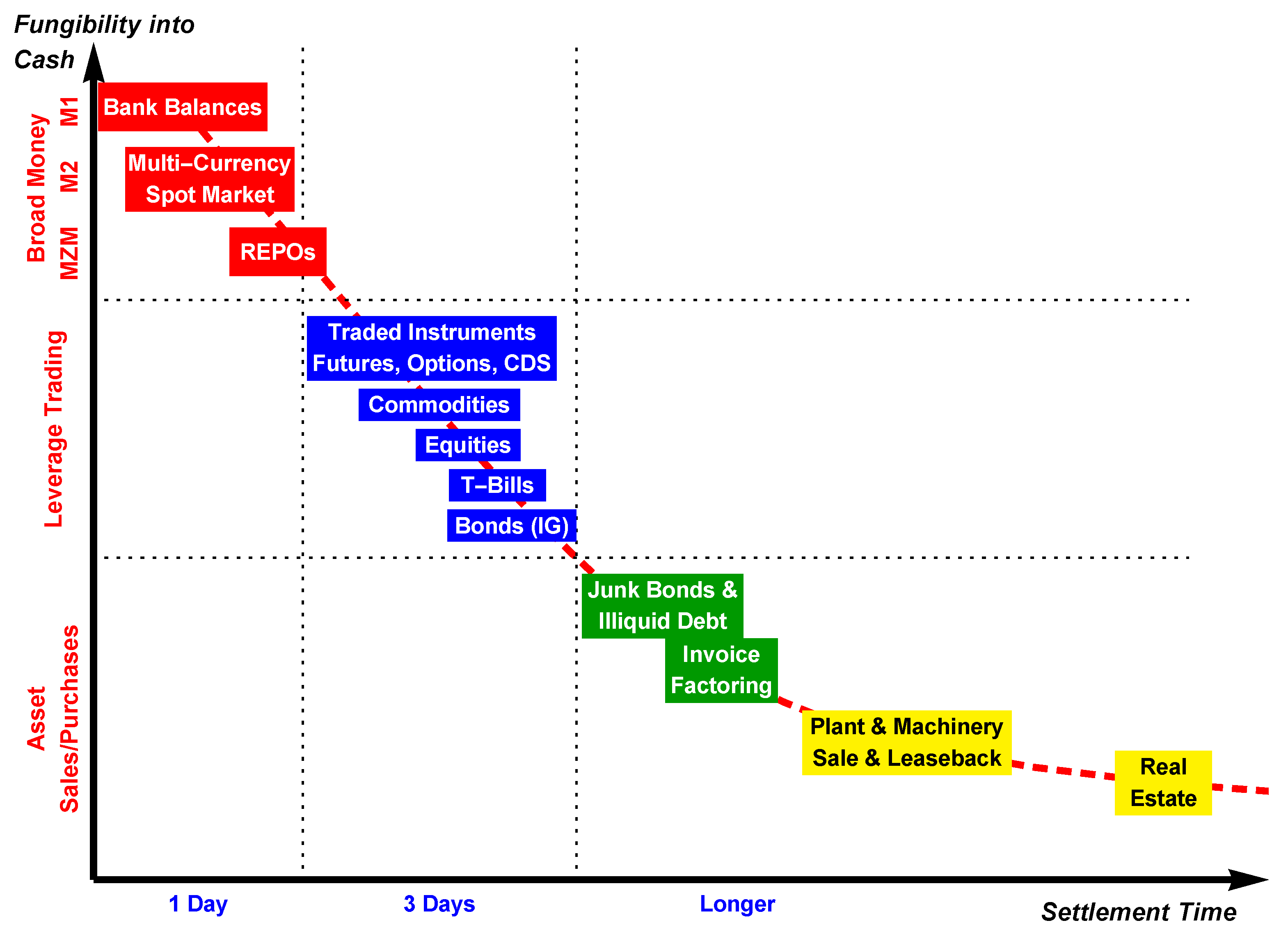
2.2. The Liquidity Continuum

As alluded to above, “formal money” is combined in today’s financial economy with significant trading platform leverage. This is expressed as the ‘liquidity continuum’ shown in Figure 5 (see also Economist (2021b) for a related discussion). This chart depicts qualitatively the inverse relationship between fungibility and maturity for some of the main financial asset classes. The size of the relevant leverage is significant, as shown in Table 1. Small retail investors access platform liquidity and leverage through brokers (such as Robinhood). These brokers carry the major platform registrations and provide the necessary margin to attract the leverage their customers trade under. Generally, financial markets perform within an overall expectation (many argue a ‘rational expectation’) that sees future growth as being in aggregate fairly similar to previous growth (for example Figure 6) adjusted for any major policy announcements, within some noise boundary. Daily movements are generally within 95% confidence limits. As demonstrated in Figure 7, over 90% of the daily changes in the S&P 500 lie within two standard deviations over a 10-year period.

2.3. The Role of Expectations

When divergence between reality and ‘rational expectations’ does occur it can be highly significant. We select two periods of such divergence to demonstrate this point, the first being the 2011 USA credit rating downgrade and the second the pandemic-induced drop in spring 2020. Markets perform differently when they are either under stress (crashing) or recovering, notwithstanding recent comments by some that recovery from the Covid-19 pandemic could be ‘V-shaped’ (Sharma et al. 2020). By contrast, the multi-period nature of a steady rise of a market index (usually termed a bull or boom market) is a more stable and predictable affair.
At market level, the dynamics of rapid change often start with a crash that is then followed by recovery. In a crash, expectations change rapidly as market participants try to protect their positions, with the recovery taking somewhat longer. Figure 8 shows how a sharp market adjustment in 2011 unfolded. The original event that led to the adjustment was a downgrading of the United States’ credit rating, with the downward phase taking rather longer to recover.
This experience differs from the Covid-19 pandemic’s impact in 2020. Once it was clear that this pandemic was going to be truly global and engulf the United States (dramatically demonstrated by the March 2020 events in New York City), financial markets started to adjust rapidly, with a ‘dash for cash’ as investors left many asset classes including United States Treasury Bills (T-Bills). The process of financial market contagion spilled across many asset classes, as asset holders first dashed for safer and more liquid assets and then for cash. This contagion drove multiple asset markets to move together, as described in a report by the Basel-based global Financial Stability Board (FinancialStabilityBoard 2020).
The US Federal Reserve reacted rapidly, buying a wide variety of assets. Figure 9 shows how after the intervention on the 23rd of March 2020 the equity market (and indeed other financial markets) stabilized, while GDP continued to fall. The cumulative impact of these changes can be seen in Figure 10, which shows rather dramatically the divergence between the real and financial economies.
The puzzle that this chart reveals is the subject of our analysis in the next section, where we present the outline of a theoretical framework to explain how the US Fed’s interventions in March 2020 stabilized financial markets but, despite injecting record amounts of new monetary assets, have failed to restart GDP in the real economy. We close the article by proposing new monetary transmission channels to directly impact the real economy from the supply side rather than the more conventionally conceived demand-side ‘helicopter money’ (Friedman 1969).

3. Discussion

3.1. The Overall Economy

Conventionally, monetary mass is defined by the domestic currency area it operates within. Central banks and national authorities measure economic activity and monetary mass within these areas, often starting from a simplified equation that relates the different elements of Gross Domestic Product (GDP):
Y = C + I + G + ( E x p I m p ) ,
where Y is the national income, C is consumption, I investment, G government expenditure (both investment, G I , and services, G S ), E x p exports, and I m p imports.
The IMF (2021) and, as implemented in the USA’s System of National Accounts the Bureau of Economic Analysis (BEA 2020a), define GDP as the sum of Gross Value Added, which can be broken down into Traded Gross Value Added (GVA), or J, where the relevant service is traded at a known market price, and Non-Traded GVA, or G N T S , where the service is provided outside the market system. Typically, G N T S covers government-supplied services such as defence or education. Therefore, government expenditure can be broken down as G = G I + G S = G I + G T S + G N T S , where ‘TS’ stands for ‘traded services’. Fundamental to this paper is to recognize that the overall economy is made up of an additional, third component, the increase in the value of asset wealth, H, over the same defined time-period. This is discussed in more detail later, but at this point we need to establish the relationship between J, G, and Y, namely:
Y = G D P = J + G N T S .
Setting (1) and (2) equal to each other and using the more granular definition for G, we get that
J = C + I + G I + G T S ,
since in this analysis we are neglecting foreign trade. To simplify our presentation, in this article we assume that all components of G are constant during the chosen time-period. This assumption allows us to ascribe all the changes in the value added in the real economy to J, thereby simplifying the need to explain the dynamics of G at every stage of our reasoning. We believe a potential future research agenda should be to relax this assumption. Table 2 shows how different kinds of economic activity contribute to the national accounts and to the increase in asset wealth in the financial economy.

3.1.1. Money, Transactions and GDP

We introduce money into this framework using the Quantity Equation (Fisher 1911):
M V = P T
or, in terms of fundamental dimensions,
[ C u r r e n c y ] C i r c u l a t i o n s T i m e = [ C u r r e n c y ] N o . o f T x T i m e or , simplifying , C u r r e n c y T i m e = C u r r e n c y T i m e .
Equation (4) relates monetary mass to economic output and applies to a specific time-period t, which may be set in advance or may fall out of the analysis, as explained below. The simplification of the dimensions shown above is due to the fact that cycles (or circulations) and number of transactions are pure numbers and are therefore dimensionless. We begin the discussion by assuming a set time-period (1 year, or 1 month, etc). In this equation, therefore, M is the quantity of money or monetary mass (see Section 3.3), V is the velocity of circulation for the given time-period, P is the average price level, and T is the total number of transactions in the given time-period. Out of these variables the one that may be less familiar is circulation, which we now define carefully because it plays an important role in what follows. ‘Circulation’ refers to the movement of money through the economy due to economic transactions and, as shown above, is measured in units of inverse time. More simply put, it is exactly analogous to a frequency, namely to the frequency of circulation of the monetary mass in a given time-period.4
In some of the economics literature GDP is used in place of T, which for dimensional consistency requires the interpretation of P as the dimensionless ‘GDP deflator’. In this paper, to account for GDP in Equation (4) in a dimensionally consistent manner we prefer to maintain the original meanings of these variables and set both sides of the equation equal to income or economic output:
x = M V = P T .
Depending on how x is interpreted, the meaning of the other variables changes. Further complexity is caused by the different definitions for monetary mass M. As definitions of monetary aggregates widen, more of the monetary mass is used in the financial economy. For the sake of clarity and completeness we list the possibilities here without worrying about the fact that some of these quantities may be challenging to measure from an econometric point of view (see also Table 3, below):
  • If x is total transaction volume (e.g., expressed in US$ transacted per year) we are dealing with the original Equation (4) and the variables are defined as above, but including also all asset purchases and sales in the financial economy. Specifically, M = Broad Money.
  • If x is GDP, then the relevant monetary mass is defined as a subset of M, namely M Y , that corresponds to the product and service transactions that actually made use of it; V and P are unchanged in concept although clearly they can change in value; and T refers only to those product and service transactions recorded within GDP. In this case we set x = Y . We note also that in this case V is dubbed the ‘income velocity of circulation’.
  • If x is set as traded GVA, or J, then our output measure no longer equates to GDP, the difference being due to non-traded GVA such as G N T S . For traded GVA we should be using Δ P = P o u t P i n in place of P, i.e., the average difference in price between two steps in the same supply chain, which measures the value added. Adopting this input/output approach allows our value-added measure to be evaluated independently of a specific stage of production, obtaining
    J = γ M V = Δ P T
    or J = M R V R = Δ P T R ,
    where the subscript R makes the emphasis on the real economy explicit and γ is a factor that expresses the fraction of the monetary mass that participates in the traded gross value-adding.
  • Finally, x could also be G N T S , non-traded GVA, whose monetary mass we call M N T S .
In our discussion we treat all components of G as constant and changes in J as changes in the real economy. J has specific quantification issues as Equation (4) is usually applied for a fixed time-period, often 1 year. Such arbitrary periods generate accounting challenges as value added in a supply chain occurs within payment transaction sequences that can straddle the initial or final time boundaries, and that can therefore lead to significant implicit stage-of-production assumptions. To address this issue we invert the algebraic problem: rather than setting the time-period and solving for V, we set the value of V and leave the time-period as a dependent variable. More precisely, following Keynes (1930) and Schumpeter (1934), we set the velocity of circulation equal to 1, which means that the activity J is measured for a single monetary circulation. For the sake of clarity, we reserve the Greek letter τ to denote the time-period that corresponds to 1 circulation, which of course can vary in different contexts.
A simple example can be provided for the case where x = G D P . If Equation (4) is applied to the US economy and a period of 1 year is chosen, the value of V is approximately 1.5, meaning that the monetary mass circulates one-and-a-half times in the US economy, in one year. If, instead, we choose to set V = 1 , then the value of GDP or Y and the corresponding time-period will become dependent variables, they will adjust to whatever corresponds to one circulation. For the US$ this is a smaller value of Y and a period shorter than 1 year.

3.1.2. The Role of Value Added

Focusing upon value added in a circulation, and relating some proportion of the monetary mass to this quantity, the productivity that value added represents can increase over time if new technologies are applied so that more output can be derived from the same level of circulation. In the short term, and ignoring economies of scale that are less important in today’s largely service-dominated economies, productivity is fixed. Using J allows us to focus on the supply side of the economy, on the assumption that an increase in consumer cash balances will be utilized in purchasing locally produced output or imports, or in saving. J looks exclusively at the first of these, and so focuses the question (to which we will return) as to how an increase in monetary mass can be used to drive an increase in value added. In reference to the Δ P in Equation (7), we define a coefficient of productivity, α , as the ratio of output to input value within a single circulation:
α = P o u t T P i n T = P o u t P i n .
It is notable that this increase in value added says nothing about possible changes in asset values or asset yields in the financial economy where, as shown in Figure 11, changes seem to be disconnected from movements in GDP.

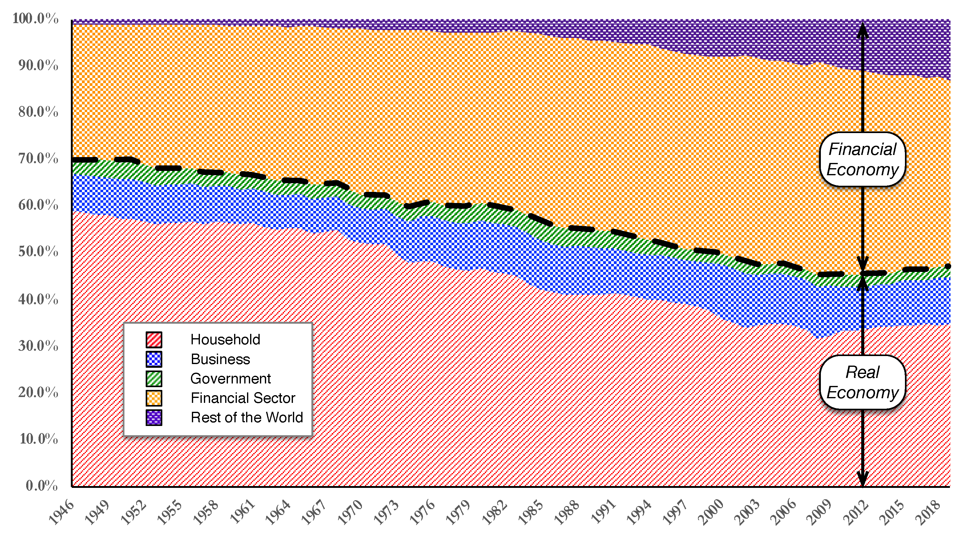
3.2. The Two Economies

Traded GVA (J) results from traded activity in the real economy. Consumers demand products and services that are provided by economic actors who in turn pay for their own inputs (raw material, labour, entrepreneurial contribution, and capital). Asset prices, on the other hand, rise in relation to investor demand. This demand may either be real (the deployment of savings) or speculative (the creation of new money for the leveraging of assets). The assets exist at the start of a circulation cycle, so financial flows into and out of them result in changes in asset prices and consequent values. Overall, rational investors are expected to optimize yield across assets in accordance with perceived risk (Markowitz 1952), although the opportunity for speculative gain (the casino referred to in Keynes (1936)) can supersede strict rationality.
These different dynamics suggest that there are two different economies coexisting within a single monetary space: the real economy, defined as the monetary circulation within which the implicated monetary mass is utilized in value-adding activity and the building of new real-capital assets, and the financial economy, defined as the monetary circulation within which the implicated monetary mass is utilized to hold and trade existing financial assets.5
Changes in regulation have also been important. During the tightly regulated 1945–1980 period, the real and financial aspects were kept in lockstep, with saving broadly matching investment across OECD countries (Feldstein and Horioka 1980). Increasingly, post-1980, a saving/investment divergence (Khan 2017; Tesar 1991) reflected increasing financializaton of developed nations’ economies, in turn associated with the post-1970 financial deregulation.6 Additionally, the introduction of the Basel Capital Accords, especially Basel II, skewed bank lending away from small firms and innovators, especially in favour of residential real estate in response to regulatory risk weights and associated bank capital allocations.
The increasing focus on wealth management (accumulation) associated with financial deregulation has led to the financialized economy becoming both pervasive (Krippner 2005) and international (Christophers 2012). We illustrated this financializaton in the US economy in Figure 1 and Figure 2. As financializaton grows, so does the divergence between the rate of return on capital investment (Keynes’s marginal efficiency of capital (Keynes 1936)) and financial economy interest rates. Expressed more formally, the marginal efficiency of capital diverges from the natural rate of interest (Wicksell 1898) which, in turn, diverges from the neutral rate of interest, which balances inflation and financial markets, as the real and financial economies become less connected in response to deregulation. Figure 12 conceptualizes the two economies and the monetary interdependencies between them.

3.2.1. Different Kinds of Circulations in the Two Economies

The two kinds of circulation that correspond to the two economies are shown in Figure 13. We note that while in the real economy there is a single circulation for a given nation-state, in the financial economy a different circulation can be identified for each asset class. Simplistically, entrepreneurs, firms, wage earners, consumers, and utility finance (banks that hold checking accounts and extend simple loans to real-economy actors) belong in the real economy. Financiers, asset traders, shadow banking, wealth management, existing real estate trading, insurance and financial options, indexes, derivatives, and other complex products belong in the financial “economies’’. Krippner (2005) usefully categorizes these as FIRE (Finance, Insurance and Real Estate) activities.
In the real economy, the output of a single circulation is the value added, J. Output in the financial economy from a single circulation is the change in the value of existing assets. To calculate the value of existing financial assets at a point in time, denoted W, one simply adds the number of each asset times its price. However, this calculation is complicated by the fact that assets come in different classes, so each class requires a separate sum. If we use i as the index that indicates the asset class, this can be expressed with a double summation as follows:
W = i = 1 n j = 1 m i p i j ,
where n is the number of asset classes, m i is the number of assets in asset class i, and p i j is the price of asset j in asset class i. The output or the ‘change in gross wealth’, H, of the financial economy can now be defined as the difference in W at the beginning of successive circulations as
H = W t + 1 W t ,
where t is used loosely as an index to indicate a given circulation rather than a specific time-period.7
Creating new assets in the real economy drives economic growth, whilst the intricacies of packaging cashflows from existing financial assets in the financial economy delivers the returns savers look for. Unsurprisingly, the monetary mass performs differently in the real and financial economies. Thus, following in the footsteps of Werner (1997, 2012), we split (4) into two components, as follows:
M R V R + M F V F = Δ P R T R + Δ P F T F ,
where the subscript R denotes the real economy and F the financial economy. The difference in the nature of the real and financial economies allows us to split (12) into two equations and set them equal to their corresponding outputs in a single circulation:8
J = M R V R = Δ P R T R
H = M F V F = Δ P F T F .
Notably, it is only Equation (13) that is integrated into the real variables described in Equation (1). Equation (14) for the financial economy is separate from the real activity variables of Consumption, Investment and Government: its connections are indirect via specific interactions between the two economies, as shown in Figure 12.
In discussing Equation (6), under our two-economy model it is possible for growth in the overall monetary mass M to exceed the growth in J without there being significantly observed consumer price inflation. This is because part of the growth in the monetary mass has been effectively ring-fenced into the financial economy, thereby inflating asset prices that are not included in mainstream price indices. Table 3 provides a summary of the different types of monetary mass for the different economic accounts.

3.2.2. Linkages Between the Real and Financial Economies
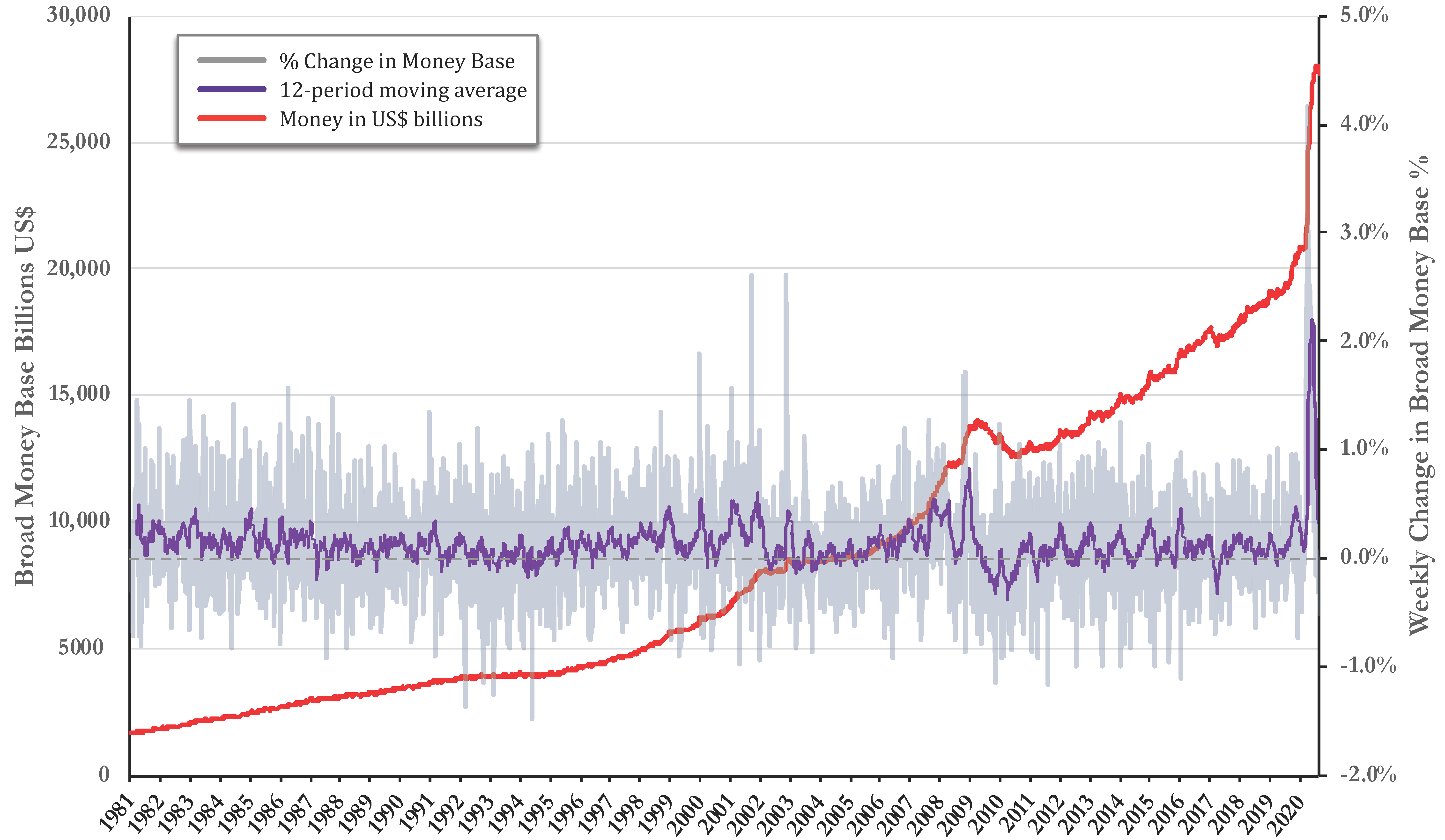
The connections9 between Equations (13) and (14) occur through a series of direct and indirect effects set out in Table 4. The same connections were also shown already at a more conceptual level in Figure 12. The financial economy’s contribution to J is defined as the impact of the value added created in the financial sector (bonuses, fees, etc.) and then as movements in consumption and investment behaviour due to the ‘wealth effect’. Drawing upon Burgess (2011), we formalize the value-added impact from the financial economy into the real economy as
J f = k P f T f + i Δ L ,
where k is the fee percentage associated with every strictly financial transaction within the monetary base, and i is the interest rate on the loan volume L in the period. We are using lower-case f to differentiate these variables from those used in Equation (14). Namely, f denotes all the financial transactions in the financial economy plus the transactions in the financial sector of the real economy (see Figure 13). Another subtle difference relative to (14) is the use of P rather than Δ P since fees are levied on gross prices rather than on price difference or value added.
Activity in the real economy is indirectly impacted also by the wealth effect, where individual economic actors may change real-economy consumption and investment behaviour as a result of changes in their financial wealth, expressed here as an unspecified functional dependence:
Δ C w = f ( H ) ,
where C w is the consumption associated with wealth effects.
A further impact from the split of the two economies, post-Keynes (1936) and Hicks (1937), is that macroeconomic adjustment is viewed by many as the result of the saving rate moving to meet the level of investment, to ensure saving equals investment (Lerner 1938). A decision to save does not mean a decision to invest in new real-economy assets, since it can be a decision to deploy cash into financial markets or hold larger cash balances. In other words, a decision to save represents a resource withdrawal from the real economy that may or may not be reinvested.10 In turn, the level of investment in the real economy depends upon (i) the desire of firms to invest to meet an anticipated market need, (ii) capability to invest from current cashflows,11 and (iii) the willingness of investors and banks to provide additional resources in preference to making potential gains on existing assets in the financial economy. Interactions in today’s globalized system with a single main reserve currency are further complicated by both the trade balance and capital flows.12
We should explain at this point that although the mathematical formalization discussed so far could be used as the starting point for a more in-depth modelling effort, for example based on extending general equilibrium theory towards dynamic behaviour (Arrow and Debreu 1954; Day 1994; Debreu 1970; Hahn 1978; Mas-Colell 1985; Samuelson 1948), etc., its role in the present paper is merely to provide greater conceptual clarity in support of the overall argument. This paper introduces innovations to monetary theory in the same discursive non-mathematical tradition used by Keynes, Friedman and others in this area. There is no claim that it is a self-standing mathematical construction of this aspect of economic theory. We therefore proceed in the same vein, with the analysis of the next building block of the two-economy model in relation to crisis: the monetary mass and how it originates.

3.3. Monetary Mass

We define the monetary mass as the quantity of money available to support economic activity in either the real economy (Equation (13)) or the financial economy (Equation (14)). In this analysis the monetary mass is assumed to be independently measured through empirical means, even if that may be difficult in practice. The monetary mass is made up of the elements set out in Table 5. We also note the importance of gross capital flows (Borio and Disyatat 2010) as a source of funds.13
Whilst both the real and financial economies require bank-mediated credit, certain forms of monetary mass are only available within the financial economy. In effect, the financial economy monetary mass consists of (i) open loan balances,14 (ii) margin deposits, (iii) trading platform leverage, and (iv) cash that a given investor has on hand and that the investor has allocated to buy positions without making use of a loan within an asset class (so this cash is now conceptually held within the asset class). By contrast, the real-economy monetary mass reflects immediately accessible cash and bank credit balances.

3.3.1. Real Economy Endogenous Money Demand

Money is created endogenously in both the real and financial economies.15 Following Hahn (1924),16 formal endogenous money creation (BOE 2014) occurs when bank balances are created from loans17 within the banking system (Werner 2014).18 Between 1959 and 2017 a link can be observed between growth in monetary aggregate M1 and GDP (Deleidi and Levrero 2019). Liquidity also matters. For instance, Laidler (2006) highlights the importance of adequate liquidity (bank deposits and cash), in turn giving central banks a lender-of-last-resort role for liquidity provision (Minsky 1982).
Expansion of the monetary mass in the real economy is a key enabler of economic growth (Schumpeter 1934). Repeated studies from as far back as the Macmillan Report of the 1930s (Stamp 1931) highlight the need for innovators, SMEs, and high-growth companies to have access to adequate capital. In theory, the ‘K plus’ rule (Friedman 1960), where the monetary mass should increase at the same percentage rate as the rate of GDP growth, should enable this expansion and ensure that inflation does not take off. Implicit to this is the requirement that the money created reaches needy firms in the real economy and is not frittered away into blowing financial economy bubbles. With the now near-complete separation between the real and financial economies, the K plus rule needs updating to reflect sophisticated capital markets, financial deregulation, banks increasingly focused on real estate lending, bond issues that are only available to large companies and private-equity companies, and the plethora of complex derivative products.

3.3.2. Financial Economy Endogenous Money Demand

For the financial economy money demand relates to the level of asset trading. Each type of asset is grouped into an asset class, which is typified by its risk and liquidity properties (see Figure 5). Financial economy money demand is the monetary mass required for a single circulation of trading for an individual asset class. The time duration of each circulation varies according to asset class (for example, real estate transactions take longer than option transactions). Abstracting and simplifying, we define eight asset classes in the financial economy:
(i)
Traded derivatives, options and futures
(ii)
Equity
(iii)
Government bonds (T-Bills/Gilts etc)
(iv)
Commercial investment-grade bonds
(v)
Non-investment-grade bonds
(vi)
Residential real estate
(vii)
Commercial real estate
(viii)
Cash
More generally, the financial sector consists of a vector of n asset classes (within which the individual assets are held) with (average) price vector p F = ( p 1 , p 2 , , p n ) . For each asset class, a specific forward price expectation ϵ i applies, the velocity of circulation is set to 1, and the time-period for a circulation is a function of price and expectation, τ i = f ( p i , ϵ i ) . Similarly, each asset class has its own monetary mass ( M F ) i . Although we chose to set V = 1 for greater conceptual clarity in the initial part of our analysis, it is easier to discuss qualitatively the instabilities in the financial economy from the point of view of a fixed time-period and a variable velocity of circulation. Specifically, the velocity of circulation of each asset class is potentially unstable, as it is a function of the price expectations ϵ i for that asset class that are, in turn, impacted by price expectations in other asset classes. This vector-based approach, therefore, provides an effective formulation to describe the effective money demand in the financial economy, which in turn drives money creation and leverage.
In the financial economy, Broad Money’s mass is augmented by the two additional concepts of ‘settlement’ and ‘trading leverage’. Settlement allows financial market traders to pay for their purchases (after netting their sales) after a typical 1 to 3-day period (Bech et al. 2020). Trading leverage relates to margin account trading, whereby a trader can leverage their collateral19 (Heimer and Simsek 2019). The repo market, where high-quality securities are sold and repurchased on a short-term basis, gives institutions access to short-term cash and specific securities required for settlement (ICMA 2020). Trading platform leverage moves pro-cyclically, so that it rises as asset prices rise and falls as asset prices fall, thereby multiplying price impacts of changes in trading expectations (Adrian and Shin 2010).

3.3.3. Exogenous Money

Since 2008, central bank money has additionally been created via QE (exogenously determined), as opposed to being related to endogenous growth. Under QE, the central bank buys existing assets (for example commercial or government bonds) that are then held on the central bank balance sheet for an indeterminate period of time. In this QE environment there is one special case where government expenditure (both consumption and investment) may be funded indirectly via the issue of government debt that is then repurchased by the central bank. Such action raises the value of G by injecting additional M1 money and is known as ‘monetary financing’ since there is little prospect of early repayment of the debt. Raising G may or may not deploy additional funds to the value-adding sector J, a point we discuss further below in the context QE transmission channels.
Following QE purchases, asset prices adjust upwards (imperfectly and with differing lags according to the “stickiness” of the asset class in question) according to demand from the central bank and as asset market actors re-balance holdings across asset classes. This rebalancing, depending on investor expectations and propensity to consume, may or may not release surpluses into the real economy.20 Mechanically, QE reduces yields, and percolates via the portfolio balance effect into other asset markets, changing prices to balance risk-adjusted yields (Joyce et al. 2011) with specific market impact set by each individual asset class’s dynamics (Goldstein et al. 2018; Thornton 2014). Significantly, investors look for safety and not to engage riskier debt.
The impact of QE on real GDP is less clear, and limited. Since QE asset purchases create new M1 deposits, which add to the real economy monetary mass, some expect that such interventions will help the real economy. However, since the sellers of the assets are financial economy actors, this provision of additional M1 money in general stays in the financial economy, raising asset prices rather than increasing traded value added J. In the UK a monetary injection of 14% of GDP was estimated to raise GDP by around 1.5% to 2.0% (Joyce et al. 2011).

3.4. The Velocity of Circulation in the Financial Economy

Effective monetary mass growth can also arise from a rise in the velocity of circulation of the monetary mass, meaning a shortened time-period τ for a single circulation. Empirically, in the short term, the velocity of circulation can be somewhat unstable, with a variety of explanations being offered (Bernanke 2006; Friedman and Schwartz 1982; Taylor 1993). Long-term, changes in the velocity (Anderson et al. 2015) occur due to a variety of structural reasons (Bordo et al. 1997; Duca 2016) that reflect the increasing sophistication of the financial economy. However, there can also be significant short-term fluctuations such as during the 1923 German hyperinflation (Laidler and Stadler 1998) and in anticipation of price changes (Cagan 1956; Hamilton 1989).
Trading volume and associated volatility (Karpoff 1987) are seen as a good proxy for length of τ i in each asset class, with volumes especially volatile in market stress.21 This creates the ‘effective τ i ’ for each circulation by asset class. Responding to market volatility, each asset class velocity itself can change rapidly and demonstrate instability in times of market stress. The overall velocity in the financial economy is itself a weighted average (based on each asset class’s proportion of M F ) of different asset class-related velocities in a specific time-period. In addition, deregulation22 has decoupled the length of cycles between the two economies and enabled a return of some of the speculative characteristics of the late 1920s.
In the face of such speculation, the financial economy is inherently unstable, since each asset class carries its own volatility ( λ ), fungibilty ( θ ) into other assets including cash, and unit of trading ( β ). Assets that have a large β account like residential property tend to have a lower fungibility parameter θ . Each asset class has its own set of time-phased expectations ( ϵ ) for each forward time-period t (or τ ), with expectations in turn relating to a function (w) expressing previous volatility in the asset class (normally through an exponentially-weighted moving average), plus some current expectation of volatility in alternative asset classes. We can express the volatility of an individual asset class as the following equation, which is weighted (u) by the monetary mass of this asset in the overall holding:
λ = i = 1 n u i λ i ϵ i .
Similarly, the average velocity of circulation of the whole financial economy is given by
V F = i = 1 n u i v i .
Arbitrage occurs across assets within an asset class vector, and then between asset classes within the vector holding all asset classes according to future price change expectations for the asset and the asset class, respectively.23 The ultimate safe asset is cash.

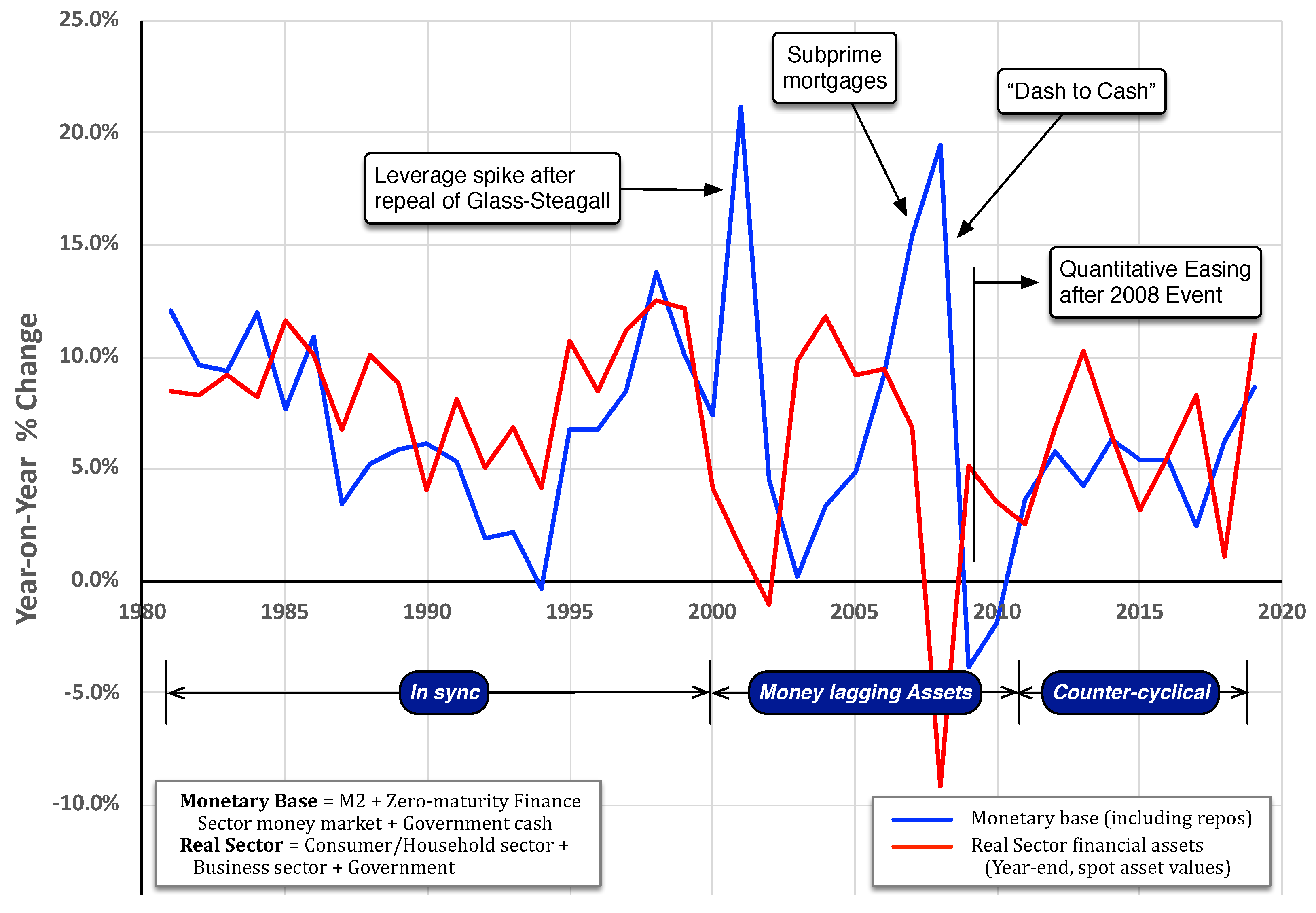
3.5. Crisis Onset and the Minsky Moment

Market stress events such as those shown in Figure 7 and Figure 8 arise when there is a need to liquidate assets to meet margin calls (Kahraman and Tookes 2020) and avoid future losses. When asset prices fall, expectations of further price falls trigger more sales in that asset class, leading to a cycle of declining prices. As asset sell-offs continue, if these pass a certain expectation threshold, they can generate a vicious cycle of contagion into adjacent asset classes, leading to an overall price crash. In other words, as volatility rises beyond the threshold in one asset class, investors move to sell assets in other asset classes that are now perceived to be vulnerable, thereby reducing the overall leverage and the associated monetary base in the financial sector. An increase in the financial economy velocity of circulation is a likely symptom of this process unfolding. This demonstrates how financial economy liquidity varies pro-cyclically in direct relation to the expected overall growth or fall in the market (Adrian and Shin 2010) and the type of asset (class) involved. When all else fails, a dash for cash results. Our financial crisis, the Minsky Moment, has arrived.
In the lead up to the Minsky Moment, financial structures become unstable because underlying cashflows from the real economy do not support financial-economy asset valuations on a systemic basis. In turn, the negative price spiral and financial contagion described above impact upon real-economy growth through associated wealth loss, loss of confidence, reductions in equity and bond flows, commercial bank lending restrictions, and loss of demand. The contagion from financial markets into real markets ceases when all financial market agents have rebalanced across asset classes to reach their new desired liquidity preference, but by then real-economy declines in aggregate demand have been triggered and economic activity is contracting. Our economic crisis has arrived.
Central banks have a mandate to prevent financial instability by intervening to moderate and stop financial contagion (Minsky 1982). In 2020, central banks used QE executed through asset purchases from the financial economy to achieve this, by providing additional liquidity and raising asset prices, reducing volatility and healing financial markets (see Figure 7, Figure 8 and Figure 9). Notwithstanding the healing delivered to the financial economy, QE had limited impact in the real economy due to the lack of automated connections between the real and financial economies (Equations (13) and (14)), and the indirect nature of the wealth effect. Figure 10 shows how, despite healing the financial economy, there was an increasing divergence from the real economy. QE had failed to reach the real economy, generating concern that inflated asset prices in the financial economy are not supported by underlying real economy cashflows and therefore represent a bubble.

3.6. Healing the Real Economy

It is by aligning the productivity and cashflows generated from value added in the real economy to asset values in the financial economy that financial stability is assured and the real economy healed. Without this alignment, crashes act as a necessary mechanism to force adjustment. In the long run market mechanisms dictate broad alignment between asset values and underlying cashflows. Adjustment can be gentle through accommodative regulation or brutal through crashes as asset price expectations realign to fundamentals (Culkin and Simmons 2019; French 1988). In spite of central banks’ best intentions, in the main, QE protects the stability of financial markets without healing the real economy and/or raising its growth rate, thereby setting up the next financial bubble and sowing the seeds of the next crash.
Avoiding this cycle of boom and bust requires mechanisms to (i) support and raise real-economy growth rates and (ii) heal the real economy in the event of a crash. The mainspring of these mechanisms is to ensure the necessary flow of capital to the entrepreneurs, innovators, SMEs, and high-growth companies to drive growth and enable cashflows in the future. Current monetary transmission channels fail to do this, given investor preferences for (i) known cashflows and (ii) making capital gains on existing assets. Additionally, de-minimus boundaries prevent smaller firms and innovators accessing capital markets, and regulatory Basel risk weights penalize certain forms of business lending and trade credit. Inadequate demand in the face of falling ‘neutral interest rates’ then drives economies into demand-deficient secular stagnation (Summers 2015). In the face of the failure of QE to heal the real economy, there are two conventional monetary responses.
First, following Friedman (1969) ‘helicopter money’ drops to consumers are made to drive activity and capital investment in the real economy. Second, in accordance with Modern Monetary Theory (MMT) and Neo-Keynesian policy, some argue that monetary-financed increases in G lift output through an increase in demand. Both proposals suffer from a lack of an automatic connection to raising long-term J and α (traded GVA and productivity), because raised consumption does not necessarily lead to higher capital investment and associated productivity increases in traded GVA. In today’s globalized world, much consumption spending is on imports that passes increase in demand to third countries instead of raising domestic value added. Additionally, with ageing populations, increases in savings can also be a significant consumer response.
Evoking a response to QE in the real economy requires targeted intervention to address three specific scenarios:
  • a shortage of liquidity (working capital) on the supply side; here targeted intervention during the same circulation should lead to a rapid upward adjustment of J, since freeing the working capital constraint should lead to a significantly larger number of supply-chain transactions;
  • a shortage of demand due to a lack of purchasing capability: this is an area that traditional helicopter money has targeted;
  • a shortage of capacity or lack of productivity on the supply side due to financing constraints on new capital investment. Investment is needed to raise both productivity and capacity of the supply side. There will be some increase in J during the same circulation due to expansion activities (building, new machinery, etc), but the increase in J will keep going in subsequent years due to the greater output that the larger capacity affords. This third intervention increases the value of our coefficient α .
These challenges call for the adoption of ‘smart helicopter money’ (Simmons et al. 2020), which is expected to be more effective in raising domestic economic growth since it directly targets an increment in J. To achieve this we identify two possible frameworks for ‘smart helicopter QE’, which can deliver monetary expansion directly to needy entrepreneurs by establishing two new QE transmission channels.
First, drawing upon the experiences of both Italian mutual credit innovator Sardex and the WIR Bank in Switzerland, locally-issued business-focused community and complementary currencies provide support to SMEs. Sardex is an electronic, account-based, non-convertible currency pegged 1:1 to the Euro and integrated into a mutual credit circuit in Sardinia that supports mainly business-to-business (B2B) transactions. WIR is a complementary currency started in 1934 only open to SMEs. Both Sardex and the WIR have been shown to make strong positive counter-cyclical growth contributions by enabling the creation of interest-free “mutual” credit by cash-starved SMEs who are underserved by the commercial banking system and modern capital markets (Dini and Kioupkiolis 2019; Littera et al. 2017; Stodder and Lietaer 2016; Studer 1998). By establishing limited convertibility for the community tokens into national currency via a QE-funded conversion fund, community credits can be integrated as an additional monetary transmission channel to target SMEs’ working-capital needs. An additional implementation of these tokens would be to issue them as a consumer helicopter drop, that forces consumers to spend the tokens with local SME businesses. We call these Smart Helicopter Tokens.
Second, QE can feed a state (or not-for-profit) fund, to finance established venture and risk capital providers with “low-cost” commercial debt funding in return for a small on-going interest payment24 and a modest share of future profits related to this finance, on condition that the funds are invested into innovators, SMEs and high-growth companies. The VCs identify and invest in such worthy companies with either equity or convertible debt, based upon firms’ business plans and anticipated enterprise valuations. The venture capital firms reap rewards through exits, dividends, further funding rounds, loan repayments, etc and they in turn repay the state/not-for-profit fund with ongoing interest, the principal, and a modest share of the related profits to help the fund build future capital reserves to support future activity (Culkin and Simmons 2018). This is a hybrid development of existing funding initiatives made by both the European Investment Bank and the British Business Bank. Table 6 summarizes the greater impacts that smart helicopter money is expected to have on increasing the output of the real economy, relative to traditional QE and other interventions.
For completeness we mention alternative interventionist central banking models visible in Asia, where ‘Structural Monetary Policy’ is used to proactively support certain sectors via shadow banks with a specific focus on stimulating demand through mainly real estate, (centrally identified) key sectors, and infrastructure development (Chen et al. 2018; Economist 2021a; Yang et al. 2019). The model has been very effective at maintaining and raising growth rates (even after 2008), but it can and does lead to overbuilding in some sectors that is then followed by consolidation. And the complex shadow banking transmission channels have from time to time needed state support to remain stable.

4. Materials and Methods

4.1. Economic Analysis

In this paper, we make extensive use of three economic concepts:
  • Circulation. The term circulation is used by both Keynes (1930) and Schumpeter (1934). In Keynes’s case he uses it to split the real from the speculative economy and as a tool to understand monetary flows and income distribution. Schumpeter uses it to express a trading flow through a series of Walrasian-type self-clearing markets.
  • Quantity Equation. We make extensive use of the Fisher (1911) Quantity Equation. This identity offers many insights when it is combined with understanding the definitional challenges relating to which transactions are implicated in a monetary circulation. Specifically, we believe that transactions associated with GDP only tell part of the story, which is why there is a need to incorporate the financial economy explicitly in the analysis.
  • Money Creation. We embrace concepts of both endogenous (Hahn 1924) and central bank exogenous (QE) (Joyce et al. 2011) money creation as being appropriate in specific settings. We do not seek or attempt to add to the very extensive literature on money demand equations.
Although temporal and time-dependent variables are discussed and although we fully acknowledge the importance of time and uncertainty in a comprehensive dynamic schema (Knight 1921), we do not address time explicitly in our analysis. This is an area for further development.

4.2. Data Sources

All our data sources are credited on the charts, and the data sets come from known credible sources, the links for which are in the bibliography. We have not undertaken complex statistical analysis, as this article is focused on developing the theory. We would welcome a follow-on econometric step of our analysis.

5. Conclusions

This paper has sought to establish through theoretical reasoning and qualitative empirical time series analysis that there is a disconnect between the real and financial economies. This disconnect, reinforced by the failure to measure changes in asset wealth in conventional output measures, has two major impacts. First, it is responsible for the inherent instability of the financial markets through the misallocation of capital into financial assets and asset bubbles. Second, it is responsible for the inefficacy of traditional QE interventions in achieving their ultimate intended goal: to restart the real economy during a crisis. In other words, the disconnect perpetrates the misallocation of capital away from innovators, SMEs and high-growth firms, thereby slowing economic growth and further raising risks of a crisis. We propose new smart helicopter QE transmission to remedy these points.
The analysis shows that our three smart helicopter money transmission channels, shown in Table 6, complement the efforts and policies to meet the current central bank imperative to maintain financial market stability, and they do this by providing monetary stimulus directly to real-economy wealth creators. The methods we advocate are tried-and-tested market mechanisms that focus support on viable growth prospects and minimize the moral hazard risks associated with state support. Our approach aligns with suggestions that central bank targeting needs to be widened from an inflation-only target to include growth and financial stability. A possible limitation of such a widening and of our approach is the extent to which institutional frameworks have evolved to integrate monetary and fiscal policy actions into single targeted interventions. Over time it is firms in the real economy and generating growth that help reduce financial market bubble pressure, since investors’ return expectations are then better met by higher cashflows created in the real economy.

Author Contributions

Conceptualization, R.S., P.D., N.C. and G.L.; methodology: R.S. and P.D.; formal analysis: P.D.; data curation: R.S. and P.D.; writing–original draft preparation, R.S. and P.D.; writing–review and editing, R.S., P.D., N.C. and G.L.; visualization: P.D. and R.S. All authors have read and agreed to the published version of the manuscript.

Funding

This research received no external funding.

Acknowledgments

Publication of this paper was financially supported by Monneta (https://monneta.org/, accessed on 18 March 2021), a German not-for-profit organization, and the Development Economics Research Group at the International Institute of Social Sciences of Erasmus University Rotterdam (https://www.iss.nl/en, accessed on 18 March 2021).

Conflicts of Interest

The authors declare no conflict of interest. P.D. worked as a part-time R&D consultant for Sardex S.p.A. from August 2016 to December 2019.

Appendix A. Definitions of Key Terms

Given the complexity of the discussion and the different interpretations of similar concepts by different schools of thought, we provide definitions of some of the key terms:
  • Collateral is pledged assets available to be sold to repay a debt.
  • Financial Economy is the set of markets where buyers and sellers trade assets for both yield and capital gain.
  • Gross Domestic Product or GDP is defined by the IMF (2021) and equals Gross Value Added which in turn equals Trading and Non-Trading Gross Value Added (J+ G N T S ).
  • Leverage is the financial multiplier that is applied to a ‘margin’ deposit in a trading account and is underpinned by collateral security held against the permitted leverage.
  • Lifetime Income, sometimes referred to as the Permanent Income Hypothesis, refers to the process economic actors use to plan savings, withdrawals and returns on assets held to allow them to optimize their income over their whole expected life.
  • Liquidity describes the free cash available to meet liabilities.
  • Liquidity Preference refers to economic actors’ preference to hold cash even if it means they miss out on financial returns that could be available from holding other assets.
  • M1 is cash and money held in ‘on-demand’ bank accounts.
  • M2 is M1 plus savings deposits, small (under US$100k) time deposits, and retail money market funds.
  • Margin is the deposit that is made into a trading account that allows the trader to trade a nominal value of specified assets that is up to some preset multiple of the deposited margin. The margin is held as immediately liquidatable security by the market maker (operator of the trading platform) against potential trading losses. Should losses exceed the required ‘margin’ amount the trader is subject to ‘margin calls’.
  • Margin Call is a demand for an additional deposit into the trading account to cover existing or anticipated trading losses.
  • Minsky Moment is when asset markets reset themselves to bring Ponzi asset financial economy valuations into line with real economy cashflows (Minsky 1989).
  • Monetary Mass is the total value of the components of broad money as defined by the IMF (2016). This includes monetary definitions that are then implemented by the US Federal Reserve for M1, M2 and MZM but that differ from the implementations by the European Central Bank and the Bank of England.
  • MZM is M2 less small-denomination time deposits plus institutional money funds US Federal Reserve System (2020a).
  • Natural Rate of Interest is the risk-adjusted interest rate that matches the Marginal Efficiency of Capital (Keynes 1936) meaning that the cost of finance equals the marginal return on capital (Wicksell 1898).
  • Neutral Rate of Interest is the rate of interest needed to keep financial markets in balance with inflation as per the central bank target inflation rate (Lavoie 2003).
  • Non-Traded Gross Value Added is the value added in the non-traded goods sector (principally government-provided services) and is represented by the symbol G N T S for ‘non-traded services’.
  • Portfolio Balance refers to the process economic actors use to mix their asset holdings so as to optimize their yield, risk and access to cash.
  • Real Economy is the set of markets in which consumers, firms, and government economic actors buy and sell products and services from each other.
  • ‘Repo’ is a short-term (often under 24 hours) agreement to sell to and (via a reverse repo) repurchase the previous repo’d security at a pre-agreed price.
  • ‘Reverse Repo’ is the original repo seller’s commitment to repurchase the security after the specified time-period.
  • Saving means national income Y minus consumption C, where consumption includes consumption by individuals, firms and households. In formal models the definition requires adjustment for capital flows.
  • Securities Settlement is the period of time specified by a trading platform between when a transaction is made and when it is netted against any others to establish an amount to be paid to or received from the agent trading.
  • Shadow Banking denotes a group of financial institutions that mediate credit to borrowers but who are not subject to banking regulations.
  • Solvency refers to the assets of an economic actor being sufficient to cover their liabilities.
  • Traded Gross Value Added represents the value added between inputs and outputs in traded goods and services and corresponds to J.
  • Velocity of Circulation is how many times the monetary mass circulates in a given period (or, more precisely, how many times each unit of account circulates, on average, in a given period). Normally V = ‘Income velocity of circulation’ and is calculated as GDP/Monetary mass, whereas in other situations V could be defined as Transaction volume/Monetary mass.
  • Wealth Effect is the indirect impact on the real economy of changes in the asset wealth of an economic actor in the financial economy.

References

  1. Adrian, Tobias, and Hyun Shin Shin. 2010. Liquidity and leverage. Journal of Financial Intermediation 19: 418–37. [Google Scholar] [CrossRef]
  2. Anderson, Richard G., Michael Bordo, and John V. Duca. 2015. Money and Velocity during Financial Crises: From the Great Depression to the Great Recession. Available online: https://www.dallasfed.org/~/media/documents/research/papers/2015/wp1503.pdf (accessed on 18 July 2020).
  3. Arrow, Kenneth J., and Gérard Debreu. 1954. Existence of an Equilibrium for a Competitive Economy. Econometrica 22: 265–90. [Google Scholar] [CrossRef]
  4. Badarudin, Z. E., Mohamed Ariff, and A. M. Khalid. 2013. Post-Keynesian money endogeneity evidence in G-7 economies. Journal of International Money and Finance 33: 146–62. [Google Scholar]
  5. BEA. 2020a. NIPA Handbook: Concepts and Methods of the U.S. National Income and Product Accounts. Available online: https://www.bea.gov/resources/methodologies/nipa-handbook (accessed on 10 February 2021).
  6. BEA. 2020b. Technical Note—Gross Domestic Product, Third Quarter of 2020 (Advance Estimate). Available online: https://www.bea.gov/sites/default/files/2020-07/gdp2q20_adv.pdf (accessed on 2 November 2020).
  7. Bech, Morten L., Jenny Hancock, Rice Tara, and Amber Wadsworth. 2020. On the Future of Securities Settlement. Technical Report, Bank of International Settlements. BIS Quarterly Review. March. Available online: https://ssrn.com/abstract=3561195 (accessed on 18 March 2021).
  8. Bernanke, Ben S. 2006. Monetary aggregates and monetary policy at the Federal Reserve: A historical perspective. Paper presented at Fourth ECB Central Banking Conference, Frankfurt, Germany, November 9–10; vol. 10. [Google Scholar]
  9. BOE. 1982. Supplementary Special Deposits Scheme. Available online: https://www.bankofengland.co.uk/-/media/boe/files/quarterly-bulletin/1982/the-supplementary-special-deposits-scheme.pdf (accessed on 16 July 2020).
  10. BOE. 2014. Money Creation in the Modern Economy. Available online: https://www.bankofengland.co.uk/quarterly-bulletin/2014/q1/money-creation-in-the-modern-economy (accessed on 4 July 2020).
  11. Bordo, Michael D., Lars Jonung, and Pierre L Siklos. 1997. Institutional Change and the Velocity of Money: A Century of Evidence. Economic Inquiry 35: 710–24. [Google Scholar] [CrossRef]
  12. Borio, Claudio, and Piti Disyatat. 2010. TGlobal imbalances and the financial crisis: Reassessing the role of international finance. Asian Economic Policy Review 5: 198–216. [Google Scholar]
  13. Burgess, Stephen. 2011. Measuring financial sector output and its contribution to UK GDP. Bank of England Quarterly Bulletin 2011: 234–46. [Google Scholar]
  14. Cagan, Phillip. 1956. The Monetary Dynamics of Hyperinflation. In Studies in the Quantity Theory of Money. Edited by Milton Friedman. Chicago: University of Chicago Press. [Google Scholar]
  15. Cartas, Jose, and Artak Harutyunyan. 2017. Compilation, Source Data, and Dissemination of Monetary Statistics. In Monetary and Financial Statistics Manual and Compilation Guide. Washington, DC: International Monetary Fund. [Google Scholar] [CrossRef]
  16. Chen, Kaiji, Jue Ren, and Tao Zha. 2018. The nexus of monetary policy and shadow banking in China. American Economic Review 108: 3891–936. [Google Scholar] [CrossRef] [Green Version]
  17. Christophers, Brett. 2012. Anaemic geographies of financialisation. New Political Economy 17: 271–91. [Google Scholar] [CrossRef]
  18. Crawford, Corrine. 2011. The repeal of the Glass-Steagall Act and the current financial crisis. Journal of Business & Economics Research (JBER) 9: 127–34. [Google Scholar]
  19. Culkin, Nigel, and Richard Simmons. 2018. Mastering Brexits Through the Ages: Entrepreneurial Innovators and Small Firms—The Catalysts for Success. Bingley: Emerald Group Publishing. [Google Scholar]
  20. Culkin, Nigel, and Richard Simmons. 2019. Shock Therapy and Entrepreneurial Flare #Brexit. International Journal of Entrepreneurial Behaviour & Research 25: 338–52. [Google Scholar]
  21. Day, Richard H. 1994. Complex Economic Dynamics. Cambridge: MIT Press, vol. 1. [Google Scholar]
  22. Debreu, Gérard. 1970. Economies with a Finite Set of Equilibria. Econometrica 38: 387–92. [Google Scholar] [CrossRef]
  23. Deleidi, Matteo, and Enrico S. Levrero. 2019. The Money Creation Process: A Theoretical and Empirical Analysis for the United States. Metroeconomica 70: 552–86. [Google Scholar] [CrossRef]
  24. Dini, Paolo, and Alexandros Kioupkiolis. 2019. The alter-politics of complementary currencies: The case of Sardex. Cogent Social Sciences 5. Available online: https://www.tandfonline.com/doi/full/10.1080/23311886.2019.1646625 (accessed on 18 March 2021). [CrossRef]
  25. Duca, John V. 2016. How capital regulation and other factors drive the role of shadow banking in funding short-term business credit. Journal of Banking & Finance 69: S10–S24. [Google Scholar]
  26. Economist. 2021a. China Leads in Precision-Guided Central Banking. Does It work? Free Exchange, February 13. [Google Scholar]
  27. Economist. 2021b. Transfer of power. Finance and Economics, February 6. [Google Scholar]
  28. FED. 2020. Money Stock Measures. H.6 Release Table 1 Footnotes. Available online: https://www.federalreserve.gov/releases/h6/current/default.htm (accessed on 18 July 2020).
  29. Feldstein, Martin. 1991. Reducing the Risk of Economic Crisis. Technical Report. Cambridge: National Bureau of Economic Research. [Google Scholar]
  30. Feldstein, Martin S., and Charles Y. Horioka. 1980. Domestic saving and international capital flows. Economic Journal 90: 314–29. [Google Scholar] [CrossRef]
  31. FinancialStabilityBoard. 2020. Holistic Review of the March Market Turmoil. Available online: https://www.fsb.org/wp-content/uploads/P171120-2.pdf (accessed on 17 November 2020).
  32. Fisher, Irving. 1911. The Purchasing Power of Money: Its Determination and Relation to Credit, Interest and Crises. New York: Macmillan. [Google Scholar]
  33. French, Kenneth R. 1988. Crash-testing the efficient market hypothesis. NBER Macroeconomics Annual 3: 277–85. [Google Scholar] [CrossRef]
  34. Friedman, Milton. 1960. A Program for Monetary Stability. New York: Fordham University Press. [Google Scholar]
  35. Friedman, Milton. 1962. Capitalism and Freedom. Chicago: Chicago University Press. [Google Scholar]
  36. Friedman, Milton. 1969. The Optimum Quantity of Money. In The Optimum Quantity of Money and Other Essays. Chicago: Adline Publishing Company, pp. 1–50. [Google Scholar]
  37. Friedman, Milton, and Anna J. Schwartz. 1982. Monetary Trends in the United States and the United Kingdom: Their Relation to Income, Prices, and Interest Rates, 1867–1975. Chicago: University of Chicago Press (for Nat. Bur. Econ. Res.). [Google Scholar]
  38. Galbraith, John Kenneth. 1961. The Great Crash, 1929: With a New Introduction by the Author. Boston: Houghton Mifflin. [Google Scholar]
  39. Goldstein, Itay, Jonathan Witmer, and Jing Yang. 2018. Following the Money: Evidence for the Portfolio Balance Channel of Quantitative Easing. Technical Report, Paper No. 2018-33. Montreal: Bank of Canada. [Google Scholar]
  40. Hahn, Frank. 1978. Exercises in Conjectural Equilibria. In Topics in Disequilibrium Economics. Edited by Steinar Strom and Lars Werin. Hoboken: Blackwell, pp. 64–80. [Google Scholar]
  41. Hahn, L. Albert. 1924. Geld und Kredit: Gesammelte Aufsätze. Tübingen: J C B Mohr. [Google Scholar]
  42. Hamilton, James D. 1989. The long-run behavior of the velocity of circulation: A review essay. Journal of Monetary Economics 23: 335–44. [Google Scholar] [CrossRef]
  43. Hayek, Friedrich A. 1960. The Constitution of Liberty. Chicago: University of Chicago Press, Available online: https://archive.org/details/in.ernet.dli.2015.553409/page/n3 (accessed on 14 November 2020).
  44. Heimer, Rawley, and Alp Simsek. 2019. Should retail investors’ leverage be limited? Journal of Financial Economics 132: 1–21. [Google Scholar] [CrossRef] [Green Version]
  45. Hicks, John R. 1937. Mr Keynes and the Classics: A suggested interpretation. Econometrica 5: 147–59. [Google Scholar] [CrossRef]
  46. ICMA. 2020. What Is Special in the Repo Market. Available online: https://www.icmagroup.org/Regulatory-Policy-and-Market-Practice/repo-and-collateral-markets/icma-ercc-publications/frequently-asked-questions-on-repo/9-what-is-a-special-in-the-repo-market/ (accessed on 10 September 2020).
  47. IMF. 2016. Monetary and Financial Statistics Manual and Compliation Guide. Available online: https://www.imf.org/~/media/Files/Data/Guides/mfsmcg_merged-web-pdf.ashx (accessed on 10 September 2020).
  48. IMF. 2017. Quarterly National Accounts Manual. Available online: https://www.imf.org/external/pubs/ft/qna/pdf/2017/QNAManual2017text.pdf (accessed on 15 February 2021).
  49. IMF. 2021. Gross Domestic Product: An Economy’s All. Available online: https://www.imf.org/external/pubs/ft/fandd/basics/gdp.htm (accessed on 15 February 2021).
  50. Joyce, Michael, Ana Lasaosa, Ibrahim Stevens, and Matthew Tong. 2011. The Financial Market Impact of Quantitative Easing in the United Kingdom. International Journal of Central Banking 7: 113–61. [Google Scholar]
  51. Joyce, Michael, Matthew Tong, and Robert Woods. 2011. The United Kingdom’s Quantitative Easing Policy: Design, Operation and Impact. Technical Report, Bank of England Quarterly Bulletin. London: Bank of England. [Google Scholar]
  52. Juniper, James, Timothy P. Sharpe, and Martin J. Watts. 2014. Modern monetary theory: Contributions and critics. Journal of Post-Keynesian Economics 37: 281–307. [Google Scholar]
  53. Kahraman, Bige, and Heather Tookes. 2020. Margin trading and comovement during crises. Review of Finance 24: 813–46. [Google Scholar]
  54. Karpoff, Jonathan M. 1987. The Relation between Price Changes and Trading Volume: A Survey. Journal of Financial and Quantitative Analysis 22: 109–26. [Google Scholar]
  55. Keynes, John M. 1930. A Treatise On Money Vols I and II. New York: Harcourt Brace. [Google Scholar]
  56. Keynes, John M. 1936. The General Theory of Employment, Interest, and Money. London: Palgrave Macmillan. [Google Scholar]
  57. Khan, Saleheen. 2017. The savings and investment relationship: The Feldstein–Horioka puzzle revisited. Journal of Policy Modeling 39: 324–32. [Google Scholar] [CrossRef]
  58. Knight, Frank Hyneman. 1921. Risk, Uncertainty and Profit. Boston: Houghton Mifflin, vol. 31. [Google Scholar]
  59. Krippner, Greta R. 2005. The financialization of the American economy. Socio-Economic Review 3: 173–208. [Google Scholar] [CrossRef]
  60. Laidler, David. 2006. Woodford and Wicksell on Interest and Prices: The place of the pure credit economy in the theory of monetary policy. Journal of the History of Economic Thought 28: 151–59. [Google Scholar] [CrossRef] [Green Version]
  61. Laidler, David, and George W. Stadler. 1998. Monetary Explanations of the Weimar Republic’s Hyperinflation: Some Neglected Contributions in Contemporary German Literature. Journal of Money, Credit and Banking 30: 816–31. [Google Scholar] [CrossRef] [Green Version]
  62. Lavoie, Marc. 2003. Measuring the natural rate of interest. Review of Economics and Statistics 85: 1063–70. [Google Scholar]
  63. Lerner, Abba P. 1938. Saving equals investment. The Quarterly Journal of Economics 52: 297–309. [Google Scholar] [CrossRef]
  64. Littera, Giuseppe, Laura Sartori, Paolo Dini, and Panayotis Antoniadis. 2017. From an Idea to a Scalable Working Model: Merging Economic Benefits with Social Value in Sardex. International Journal of Community Currency Research 21: 6–21. Available online: https://ijccr.files.wordpress.com/2017/02/littera-et-al.pdf (accessed on 18 March 2021).
  65. Lucas, Robert E., Jr. 1976. Econometric Policy Evaluation: A Critique. In The Phillips Curve and Labor Markets. Edited by Karl Brunner and Alan Meltzer. Carnegie Rochester Conference Series; New York: North Holland, pp. 19–46. [Google Scholar]
  66. Markowitz, Harry M. 1952. Portfolio selection. Journal of Finance 7: 77–91. [Google Scholar]
  67. Mas-Colell, Andreu. 1985. The Theory of General Economic Equilibrium: A Differentiable Approach. Cambridge: Cambridge University Press. [Google Scholar]
  68. Minsky, Hyman P. 1982. Can “It” Happen Again?: Essays on Instability and Finance. Armonk: M.E. Sharpe. [Google Scholar]
  69. Minsky, Hyman P. 1989. The Financial Instability Hypothesis: A Clarification. Ph.D. Thesis, Bard College, Annandale-On-Hudson, NY, USA. Available online: http://digitalcommons.bard.edu/hm_archive/145 (accessed on 28 August 2020).
  70. Muth, John F. 1961. Rational Expectations and the Theory of Price Movements. Econometrica 29: 315–35. [Google Scholar] [CrossRef]
  71. NASDQ. 2020. SPX Historical Data. Available online: https://www.nasdaq.com/market-activity/index/spx/historical (accessed on 2 November 2020).
  72. Obstfeld, Maurice, and Alan M. Taylor. 2005. Global Capital Markets: Integration, Crisis, and Growth. Cambridge: Cambridge University Press. [Google Scholar]
  73. Samuelson, Paul A. 1948. Economics, an Introductory Analysis. New York: McGraw-Hill. [Google Scholar]
  74. Schumpeter, Joseph. 1934. The Theory of Economic Development. Cambridge: Harvard University Press. [Google Scholar]
  75. Sharma, Dhruv, Jean-Phillipe Bouchaud, Stanislao Gualdi, Marco Tarzia, and Francesco Zamponi. 2020. “V-, U-, L-or W-shaped recovery after COVID?” Insights from an Agent-Based Model June 2020 SSRN 3627505. Available online: https://arxiv.org/pdf/2006.08469.pdf (accessed on 22 November 2020).
  76. Sifma. 2020. US Repo Market Fact Sheet. Available online: https://www.sifma.org/resources/research/us-repo-market-fact-sheet/ (accessed on 10 September 2020).
  77. Simmons, Richard, Giuseppe Littera, Nigel Culkin, Paolo Dini, Luca Fantacci, and Massimo Amato. 2020. Helicopter, Bazooka or Drone? Economic Policy for the Coronavirus Crisis. Available online: https://www.politico.eu/article/helicopter-bazooka-drone-economic-policy-coronavirus-crisis-money// (accessed on 10 February 2021).
  78. Stamp, Josiah C. 1931. The report of the Macmillan Committee. The Economic Journal 41: 424–35. [Google Scholar] [CrossRef]
  79. Stodder, James, and Bernard Lietaer. 2016. The Macro-Stability of Swiss WIR-Bank Credits: Balance, Velocity, and Leverage. Comparative Economic Studies 58: 570–605. [Google Scholar] [CrossRef]
  80. Studer, Tobias. 1998. IWIR and the Swiss National Economy. Basel: WIR Bank. [Google Scholar]
  81. Summers, Lawrence H. 2015. Demand side secular stagnation. American Economic Review 105: 60–65. [Google Scholar] [CrossRef] [Green Version]
  82. Tarassow, Artur. 2019. Forecasting US money growth using economic uncertainty measures and regularisation techniques. International Journal of Forecasting 35: 443–57. [Google Scholar] [CrossRef]
  83. Taylor, John B. 1993. Discretion versus policy rules in practice. In Carnegie-Rochester Conference Series on Public Policy. North-Holland: Elsevier, vol. 39, pp. 195–214. [Google Scholar]
  84. Tesar, Linda L. 1991. Savings, investment and international capital flows. Journal of International Economics 31: 55–78. [Google Scholar] [CrossRef]
  85. Thornton, Daniel L. 2014. QE: Is There a Portfolio Balance Effect? Technical Report, Review 96, No. 1. St. Louis: Federal Reserve Bank of St. Louis. [Google Scholar]
  86. US Federal Reserve System. 2020a. Institutional Money Funds [WIMFNS], M2 Money Stock [WM2NS], Total Cash Balance [GDTCBW], General Account Balance at Federal Reserve [GDBFRW], Time and Savings Deposits at Commercial Banks [GDTSDCBM] & Demand Deposits at Commercial Banks [GDDDCBW] Money Zero Maturity [MZM]. Retrieved from FRED, Federal Reserve Bank of St. Louis. Available online: https://fred.stlouisfed.org/series/NBCB (accessed on 9 September 2020).
  87. US Federal Reserve System. 2020b. Quarter 2, 2020, Z.1 Financial Accounts of the United States (Sept 21, 2020). Available online: https://www.federalreserve.gov/apps/fof/FOFTables.aspx (accessed on 1 October 2020).
  88. Werner, Richard. 1997. Towards a New Monetary Paradigm: A Quantity Theorem of Disaggregated Credit, with Evidence from Japan. Kredit und Kapital 2: 276–309. [Google Scholar]
  89. Werner, Richard. 2012. Towards a New Research Programme on ‘Banking and the Economy’—Implications of the Quantity Theory of Credit for the Prevention and Resolution of Banking and Debt Crises. International Review of Financial Analysis 25: 1–17. [Google Scholar]
  90. Werner, Richard. 2014. How do banks create money, and why can other firms not do the same?An explanation for the coexistence of lending and deposit-taking. International Review of Financial Analysis 36: 71–77. [Google Scholar] [CrossRef] [Green Version]
  91. Wicksell, Knut. 1898. Interest and Prices. Translated by Richard Kahn. London: Macmillan for the Royal Economic Society. [Google Scholar]
  92. Yang, Liu, Sweder van Wijnbergen, Xiaotong Qi, and Yuhuan Yi. 2019. Chinese shadow banking, financial regulation and effectiveness of monetary policy. Pacific-Basin Finance Journal 57: 101169. [Google Scholar] [CrossRef]
1.
They argue that this unlimited capability is due to the supremacy of state-issued money, meaning that government debt should be seen as a financial asset for the private sector, not as a liability.
2.
This article draws on many of the same concepts and is complementary but not intended as a specific follow-on to Werner’s work.
3.
Please see Appendix A for definitions of technical terms.
4.
For conceptual clarity, we assume that M is constant during the time-period used to calculate these variables.
5.
Although we do not treat it in this article, as already mentioned the duration of a circulation can differ between the real and financial economies.
6.
This savings/investment divergence is not associated with trade balance changes (Obstfeld and Taylor 2005).
7.
As already stated, the implication is that the time duration of different circulations may be different, but this does not present a problem in the present analysis.
8.
This is a major modelling step as it represents a strict additional constraint whose validity will need to be verified ex post by future empirical and mathematical research. This paper presents only the first tentative steps towards a possible model, modulated by the interactions shown in Figure 12 and Table 4, which could be expressed as additional equations.
9.
In mathematics or physics this is called the ‘coupling’.
10.
We note that changes in post-Pandemic saving behaviour are not yet clear.
11.
In the macroeconomic identity for saving this diversion of funds to investment is seen as saving deployed as investment.
12.
In a dynamic setting, to these must be added the import propensity to consume (how much of each $ of national income is spent on imports vs. home production) and the propensity to save (how much of each additional $ of income is saved).
13.
Capital flows have special importance with respect to exchange rate constraints on central bank policy.
14.
Open loan balances mean the amount of credit still available to be drawn down by the economic actor.
15.
Since the 1970s, money has been created endogenously in both the real and financial economies unless there are ‘emergency’ administrative constraints (Badarudin et al. 2013), such as the UK 1973 Supplementary Special Deposits Scheme (BOE 1982) where credit creation levels were specified by the central bank.
16.
L Albert Hahn had considerable influence on Josef Schumpeter.
17.
Banks and central banks are the only institutions able to create official national currency.
18.
The exception to this is when trading platforms (which may or may not be part of banks) create trading liquidity through margin trading prior to platform netting and settlement of any outstanding liabilities.
19.
Professional traders in the USA are limited to a 1:50 leverage by the Dodd Frank Act of 2010, whilst commodity traders have a leverage limit of 1:20.
20.
Surpluses can be reinvested into financial assets in anticipation of further price rises.
21.
Short-term τ changes can be later reflected into M2 changes (Tarassow 2019).
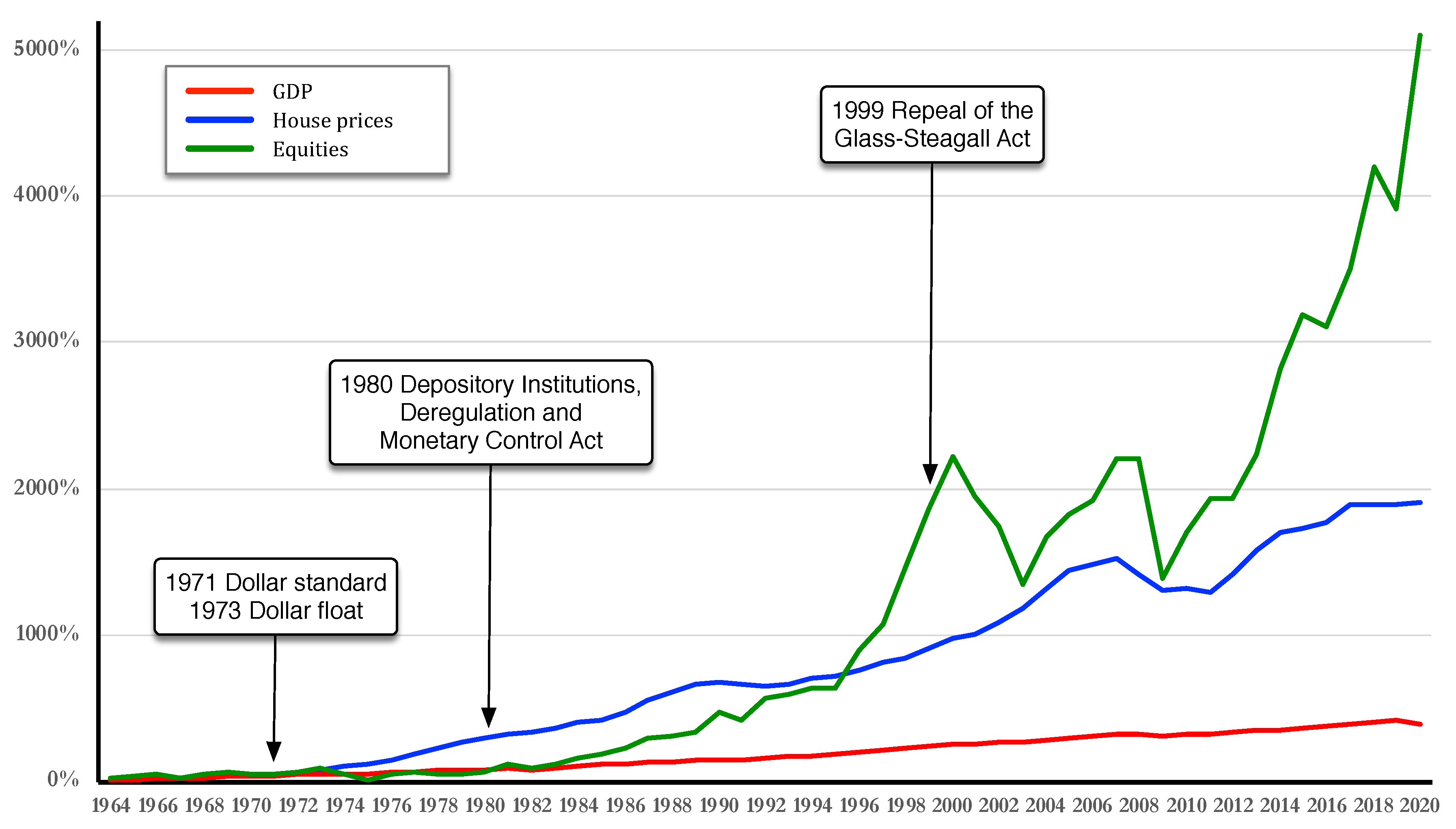
22.
Onset of the Euro-Dollar market in the 1960s, the dollar standard from 1971, the Depository Institutions Deregulation and Monetary Control Act of 1980, and the 1999 repeal of the Glass-Steagall Act.
23.
Each asset carries a future price change expectation, either “inheriting” this from the asset class or having its own expectation. For example, in late January 2021 GameStop had a different and more extreme price expectation than that of its asset class.
24.
Say 50 or 100 basis points over the costs of the funds.
Figure 1. Growth in US Dollar financial assets, cumulative view (US Federal Reserve System 2020b).
Jrfm 14 00129 g001
Figure 2. Cumulative % share of US financial assets by sector (US Federal Reserve System 2020b).
Jrfm 14 00129 g002
Figure 3. Growth in the United States’ monetary base (M2 + MZM + Government holdings).
Jrfm 14 00129 g003
Figure 4. US Monetary and Real Economy Growth 1980–2020 (Sifma 2020; US Federal Reserve System 2020b).
Jrfm 14 00129 g004
Figure 5. The Liquidity Continuum: variation of monetary, financial-leverage, and real-asset fungibility vs. settlement time.
Jrfm 14 00129 g005
Figure 6. 90-Day smoothed change in S&P Index 2010–2020 (NASDQ 2020).
Jrfm 14 00129 g006
Figure 7. Daily % variation in S&P Index 2010–2020 (NASDQ 2020).
Jrfm 14 00129 g007
Figure 8. Daily % variation in S&P Index, 2011 Crash (NASDQ 2020).
Jrfm 14 00129 g008
Figure 9. Daily % variation in S&P Index during the 2020 pandemic (BEA 2020b; NASDQ 2020).
Jrfm 14 00129 g009
Figure 10. Cumulative % change in S&P Index during the 2020 pandemic (BEA 2020b; NASDQ 2020).
Jrfm 14 00129 g010
Figure 11. Comparison of percentage change in asset prices (residential house prices and S&P 500 equities vs. GDP, United States).
Jrfm 14 00129 g011
Figure 12. Structure of the two economies, high-level monetary flow connections, and wealth effect.
Jrfm 14 00129 g012
Figure 13. Circulation.
Jrfm 14 00129 g013
Table 1. Leverage in the US financial economy at the end of 2019 (US Federal Reserve System 2020b).
US$b
M11446
M22399
MZM3130
Broad Money8068
Broad Money leveraged to:
    Futures22,709
    Options45,417
    CDS3000
    Commodities1000
    Equities1771
    Total73,897
Leverage Factor916%
Table 2. Contribution of economic activities to the national accounts (IMF 2017).
Contribution to ...
Productive Value AddedNon-Traded ServicesGDP CalculationWealth Calculation
SectorJGGDP ( J + G N T S )H
Agriculture and ForestryYesNoYesNo
FishingYesNoYesNo
Mining and QuarryingYesNoYesNo
ManufacturingYesNoYesNo
Electricity, Gas, Steam & Air ConditioningYesNoYesNo
Water SupplyYesNoYesNo
ConstructionYesNoYesNo
Wholesale and RetailYesNoYesNo
Transportation and StorageYesNoYesNo
AccommodationYesNoYesNo
Food ServicesYesNoYesNo
Information and CommunicationYesNoYesNo
Financial and Auxiliary ServicesYesNoYesNo
Insurance and PensionsYesNoYesNo
Real Estate ServicesYesNoYesNo
Professional, Scientific and Technical Serv.YesNoYesNo
Administration and Support ServicesYesNoYesNo
Public Admin., Defence, Social SecurityNoYesYesNo
EducationNoYesYesNo
Human Health and Social Work (Gov.)NoYesYesNo
Human Health and Social Work (Private)YesNoYesNo
Arts, Entertainment and RecreationYesNoYesNo
Asset Value ChangesNoNoNoYes
Table 3. Monetary mass variables associated with different economic accounts during one circulation.
AccountAccount VariableMass VariableRelation to Other Mass Variables
Whole economyTot. Transac. Vol.M M R + M N T S + M F = M Y + M F = Broad Money
GDPY M Y M M F = M R + M N T S
Traded GVAJ M R M ( M N T S + M F ) = M Y M N T S = γ M
Non-traded Govt. GVA G N T S M N T S M ( M R + M F ) = M Y M R
Change in gross wealthH M F M M Y
Table 4. Impacts of monetary flows on real and financial economies.
Real EconomyFinancial Economy
ImpactImpact
FlowGDP M R Asset Valuation M F Impact TypeAssumptions
Savings-++DirectAll new savings deployed into financial assets
Savings withdrawal-+DirectAll savings withdrawals taken from assets
Equity investment+ (indirect)++DirectFunded by existing, not new money
Bond issue-++DirectFunded by existing, not new money
Profit and loan interest-++DirectAssumes reinvestment of proceeds received
Management charges++DirectAssumes funded by reduced reinvestment of profits
Savings returns++DirectAssumes funded by reduced reinvestment of profits
Inbound capital flow--++DirectAll deployed into financial assets
Outbound capital flow--DirectAll withdrawn from assets
Wealth effectIf > 0 it can increase consumption and vice versaIndirect
Table 5. Components of the monetary mass.
NameDescriptionReal EconomyFinancial EconomySource
M1Physical notes and coins, and money in current accounts at banksYesYesFED (2020)
M2M1 + savings, small time deposits, and retail money market fundsYesYesFED (2020)
Broad MoneyM2 + eligible debt securities (paper that can be repo’d). In the USA this includes MZM.PartialYesTable 61, p. 182 in IMF (2016)
Net Broad MoneyBroad Money − M2NoYes
MZM(M2 − small term-deposits) + institutional money market fundsNoYesUS Federal Reserve System (2020a)
Trading LeverageCreation of trading credits against margin depositsNoYes
Table 6. Impacts of different monetary policy interventions.
Impact on:Real EconomyMonetary MassLeakagesOther
InterventionMethodCTraded GVAnon- TGVAMReal Econ.Fin. Econ. I m p Saving α (Prod- uctivity)Capital Gain
Additional working capitalMutual credit +
VC Conv. Debt + ++
Friedman helicopter dropCash to consumers++ +++++?
Smart helicopter working capitalConvertible tokens + +++++?
Smart helicopter tokensTokens for domestic spend++ +++ +?
Smart helicopter investment cashVC equity & debt + ++ ?+?
Conventional QEAsset purchases + + +
Rise in GMMT ?+ + ?
Structural monetary policyAsian development model + +++? ??
Publisher’s Note: MDPI stays neutral with regard to jurisdictional claims in published maps and institutional affiliations.

