Pricing Perpetual American Put Options with Asset-Dependent Discounting

Abstract

The main objective of this paper is to present an algorithm of pricing perpetual American put options with asset-dependent discounting. The value function of such an instrument can be described as $V_{{\mathrm{A}}^{\mathrm{Put}}}^{\omega }(s)={sup}_{\tau \in \mathcal{T}}{\mathbb{E}}_s[e^{-{\int }_0^{\tau }\omega (S_w)dw}{(K-S_{\tau })}^{+}],$ where $\mathcal{T}$ is a family of stopping times, $\omega$ is a discount function and $\mathbb{E}$ is an expectation taken with respect to a martingale measure. Moreover, we assume that the asset price process $S_t$ is a geometric Lévy process with negative exponential jumps, i.e., $S_t=s{e}^{\zeta t+\sigma B_t-{\sum }_{i=1}^{N_t}{Y}_i}$. The asset-dependent discounting is reflected in the $\omega$ function, so this approach is a generalisation of the classic case when $\omega$ is constant. It turns out that under certain conditions on the $\omega$ function, the value function $V_{{\mathrm{A}}^{\mathrm{Put}}}^{\omega }(s)$ is convex and can be represented in a closed form. We provide an option pricing algorithm in this scenario and we present exact calculations for the particular choices of $\omega$ such that $V_{{\mathrm{A}}^{\mathrm{Put}}}^{\omega }(s)$ takes a simplified form.

1. Introduction

In this paper, we consider a perpetual American put option with asset-dependent discounting. We consider a standard stochastic background for this problem, i.e., we define a complete filtered risk-neutral probability space $(\mathsf{\Omega },\mathcal{F},{\left\{{\mathcal{F}}_t\right\}}_{t\ge 0},\mathbb{P})$, on which we define the asset price process $S_t$. Then, ${\mathcal{F}}_t$ is a natural filtration of $S_t$ satisfying the usual conditions and $\mathbb{P}$ is a risk-neutral measure under which the discounted (with respect to the risk-free interest rate $r>0$) asset price process $e^{-rt}{S}_t$ is a local martingale. A family of ${\mathcal{F}}_t$-stopping times is denoted by $\mathcal{T}$ while ${\mathbb{E}}_s$ denotes the expectation with respect to $\mathbb{P}$ when $S_0=s=e^x$. The value function of the perpetual American put option with asset-dependent discounting can be represented by

$$V_{{\mathrm{A}}^{\mathrm{Put}}}^{\omega }(s):=\underset{\tau \in \mathcal{T}}{sup}{\mathbb{E}}_s\left[e^{-{\int }_0^{\tau }\omega (S_w)dw}{(K-S_{\tau })}^{+}\right].$$

(1)

The asset-dependent discounting is reflected in the $\omega$ function, which is our key concept considered in this article. We underline here that the discount function $\omega$ for various economical reasons can be different from the risk-free interest rate $r>0$; see Al-Hadad and Palmowski (2021) for further explanation. The way we choose discounting is to model strong dependence of discount factor with the asset price. The goal is to understand various economical phenomena that might appear in this extreme case. Our approach differs from typical studies considered in the literature, where the interest rate is independent from the asset price or there is a weak dependence between these two factors. Therefore, this research is noteworthy not only in the context of option pricing, but also in other areas where optimisation problems appear.

Our main motivation comes from the work of Linetsky (1999) who considers up-and-out put options traded mainly over-the-counter. In these options, the discounting factor depends exponentially on the cumulative excursion time above or below a given barrier during the entire life of the option. In other words, $\omega (s)=\varrho {𝟙}_{\{s\in A(H)\}}$ where $A(H)=\{s\ge 0:\pm (s-H)\ge 0\}$. Similar step-like options were considered in Rodosthenous and Zhang (2018) where the discounting is related to the occupation time of the asset price below a fixed level y exceeding an independent exponential random variable with mean $1/\varrho$. This discounting corresponds to the special choice of $\omega (s)=r+\varrho {𝟙}_{\{s\le y\}}$, where r is a risk-free interest rate. In general, one can think of $\omega (S_t)$ as the general knock-out (or knock-in) rate depending on the asset price of some vanilla options. This additional feature might allow us to customise the financial product according to the demand of the risk management.

Moreover, we assume that the asset price process $S_t$ is a geometric Lévy process with negative exponential jumps, i.e.,

$$S_t:=s{e}^{X_t}$$

(2)

with

$$X_t:=\zeta t+\sigma B_t-\sum _{i=1}^{N_t}{Y}_i,$$

(3)

where $\zeta$ and $\sigma >0$ are constant, $N_t$ is the Poisson process with intensity $\lambda \ge 0$ independent of Brownian motion $B_t$, and ${\left\{Y_i\right\}}_{i\in \mathbb{N}}$ are i.i.d. random variables independent of $B_t$ and $N_t$ having exponential distribution with mean $1/\phi >0$. Under the martingale measure $\mathbb{P}$, the drift parameter is of the form

$$\zeta :=r-\frac{{\sigma }^2}{2}+\frac{\lambda }{\phi +1}.$$

Note that when $\lambda =0$, then we end up with the classical Black–Scholes model. However, empirical studies show that stock prices have a heavier left tail than normal distribution. Note that the negative jumps underline the market crashes that appear once per while. Therefore, nowadays many books and articles concern, as we do in this work, pricing of derivative securities in market models based on Lévy processes; see Cont and Tankov (2004) for more details. Still, to get a complete picture, we analyse here the case of $\lambda =0$ as well. Our model of asset price is a particular case of the Kou model where the logarithm of the price process is a jump diffusion; see Kou (2002).

The main objective of this paper is to present an algorithm of pricing perpetual American put options with asset-dependent discounting with the value function defined in (1) and the asset price process $S_t$ given in (2). Furthermore, we take into account some specific scenarios (e.g., when $\sigma =0$ or $\lambda =0$), and, for these cases, we are able to derive analytical forms of the value function, while for more complex examples, we show how to handle them numerically.

Detailed theoretical results of the analysed problem were already developed in Al-Hadad and Palmowski (2021), where the authors presented the approach of deriving a closed form of value function (1) for even a more general setting than it is considered here. Therefore, in this paper, we focus more on numerical side of this problem and analyse, in detail, a few particular cases where more explicit results can be derived.

Still, before we present the option pricing method in our set-up, we recall the most important theoretical issues on which our article is based on. A key step in deriving a closed form of (1) is identifying the form of the optimal stopping rule ${\tau }^{*}$ for which the supremum in (1) is attained. It turns out that under certain conditions on the discount function $\omega$, which are presented in the next section, the value function is convex. By combining this fact with the classical optimal stopping theory presented, e.g., in Peskir and Shiryaev (2006), it allows us to conclude that the optimal stopping region is an interval $[l^{*},u^{*}]$ and hence

$${\tau }^{*}=inf\{t\ge 0:S_t\in [l^{*},u^{*}]\}$$

for some optimal thresholds $l^{*}\le u^{*}$. Observe that for the non-negative discount function $\omega$, we have $l^{*}=0$ (since waiting is not beneficial). Therefore, in this case a single continuation region appears. In general, for the negative $\omega$, we can observe a double continuation region; for more details, see De Donno et al. (2020).

The optimal boundary levels $l^{*}$ and $u^{*}$ can be found by application of standard methods of maximising the function

$$v_{{\mathrm{A}}^{\mathrm{Put}}}^{\omega }(s,l,u):={\mathbb{E}}_s\left[e^{-{\int }_0^{{\tau }_{l,u}}\omega (S_w)dw}{(K-S_{{\tau }_{l,u}})}^{+}\right]$$

over l and $u>l$. To find $v_{{\mathrm{A}}^{\mathrm{Put}}}^{\omega }(s,l,u)$, we use exit identities for spectrally negative Lévy processes containing so-called omega scale functions introduced in Li and Palmowski (2018).

As shown in (Al-Hadad and Palmowski 2021, Theorem 9), another way of finding the optimal thresholds $l^{*}<u^{*}$ is to apply the classical smooth and continuous fit conditions.

Typically, a price of the option is a solution to a certain Hamiltonian–Jacobi–Bellman (HJB) system, and the optimal thresholds are identified using the smooth fit conditions. We want to underline that our approach is different, although still finding the omega scale functions is carried out via solving certain ordinary differential equations.

The paper is organised as follows. In Section 2, we introduce basic theory and notation. Section 2.4 provides the main theoretical results of this paper. In Section 3, we present some specific examples where the option price can be expressed in the explicit way. Section 4 focuses on the purely numerical analysis. We also show there that these two approaches are consistent. The last section includes our conclusions.

2. Preliminaries

2.1. Assumptions

It the beginning, we note that the analysed American put option will not be realised when its payoff is equal to 0. Hence, we can transform the form of the value function given in (1) into the following one

$$V_{{\mathrm{A}}^{\mathrm{Put}}}^{\omega }(s):=\underset{\tau \in \mathcal{T}}{sup}{\mathbb{E}}_s\left[e^{-{\int }_0^{\tau }\omega (S_w)dw}(K-S_{\tau })\right].$$

(4)

We work under the same assumptions as those formulated in (Al-Hadad and Palmowski 2021, Section 2.2). However, this time we consider slightly more specific assumptions on the $\omega$ function, namely, that

Assumption 1.

A discount function ω is concave, nondecreasing and bounded from below.

From (Al-Hadad and Palmowski 2021, Remark 3) we can then conclude that under Assumption 1, the value function $V_{{\mathrm{A}}^{\mathrm{Put}}}^{\omega }(s)$ is convex.

2.2. Optimal Stopping Time

From (Al-Hadad and Palmowski 2021, Section 2.4), it follows that the optimal exercise time is the first entrance of the process $S_t$ into some interval, that is, it has the following form

$${\tau }_{l,u}=inf\{t\ge 0:S_t\in [l,u]\}.$$

Hence, we can represent value function (4) as

$$V_{{\mathrm{A}}^{\mathrm{Put}}}^{\omega }(s)=v_{{\mathrm{A}}^{\mathrm{Put}}}^{\omega }(s,l^{*},u^{*}),$$

where

$$v_{{\mathrm{A}}^{\mathrm{Put}}}^{\omega }(s,l^{*},u^{*}):=\underset{0\le l\le u\le K}{sup}{v}_{{\mathrm{A}}^{\mathrm{Put}}}^{\omega }(s,l,u)$$

and

$$v_{{\mathrm{A}}^{\mathrm{Put}}}^{\omega }(s,l,u):={\mathbb{E}}_s\left[e^{-{\int }_0^{{\tau }_{l,u}}\omega (S_w)dw}(K-S_{{\tau }_{l,u}})\right].$$

(5)

Moreover, we denote the optimal stopping time by

$${\tau }^{*}:={\tau }_{l^{*},u^{*}},$$

where $l^{*}$ and $u^{*}$ realise the supremum above. As shown in (Al-Hadad and Palmowski 2021, Theorem 9), another way of identifying the critical points $l^{*}$ and $u^{*}$ can be achieved via application of the smooth fit property. In that case, $l^{*}$ and $u^{*}$ satisfy

$${(V_{{\mathrm{A}}^{\mathrm{Put}}}^{\omega })}^{\prime }(u^{*})=-1\mathrm{and}{(V_{{\mathrm{A}}^{\mathrm{Put}}}^{\omega })}^{\prime }(l^{*})=-1.$$

(6)

2.3. Scale Functions

By applying the fluctuation theory of Lévy processes, we can find a closed form of (5), and hence of (4), in terms of the so-called omega scale functions.

To introduce them formally, first let us define the Laplace exponent of $X_t$ via

$$\psi (\theta ):=\frac{1}{t}log\mathbb{E}[e^{\theta X_t}\mid X_0=0],$$

which is well-defined for $\theta \ge 0$ since our $X_t$ is a spectrally negative Lévy process. In the case of $X_t$ given in (3), the Laplace exponent takes the form

$$\psi (\theta )=\zeta \theta +\frac{{\sigma }^2}{2}{\theta }^2-\frac{\lambda \theta }{\phi +\theta }.$$

(7)

By $\mathsf{\Phi }(q)$, we denote the right inverse of $\psi (\theta )$, i.e.,

$$\mathsf{\Phi }(q):=sup\{\theta \ge 0:\psi (\theta )=q\},$$

where $q\ge 0$.

The first scale function $W^{(q)}(x)$ is defined as a continuous and increasing function such that $W^{(q)}(x)=0$ for all $x<0$, while for $x\ge 0$, it is defined via the following Laplace transform

$${\int }_0^{\infty }{e}^{-\theta x}{W}^{(q)}(x)dx=\frac{1}{\psi (\theta )-q}$$

(8)

for $\theta >\mathsf{\Phi }(q)$. We define also the related scale function $Z^{(q)}(x)$ by

$$Z^{(q)}(x):=1+q{\int }_0^x{W}^{(q)}(y)dy,$$

where $x\in \mathbb{R}$. From Cohen et al. (2013), we know that for $X_t$ given in (3), we have

$$W^{(q)}(x)=\frac{e^{{\gamma }_{1}x}}{{\psi }^{\prime }({\gamma }_1)}+\frac{e^{{\gamma }_{2}x}}{{\psi }^{\prime }({\gamma }_2)}+\frac{e^{\mathsf{\Phi }(q)x}}{{\psi }^{\prime }(\mathsf{\Phi }(q))},$$

(9)

where $\{{\gamma }_1,{\gamma }_2,\mathsf{\Phi }(q)\}$ is the set the real solutions to $\psi (\theta )=q$. In turn, $Z^{(q)}(x)$ is as follows

$$Z^{(q)}(x)=1+q\left(\frac{e^{{\gamma }_{1}x}-1}{{\gamma }_1{\psi }^{\prime }({\gamma }_1)}+\frac{e^{{\gamma }_{2}x}-1}{{\gamma }_2{\psi }^{\prime }({\gamma }_2)}+\frac{e^{\mathsf{\Phi }(q)x}-1}{\mathsf{\Phi }(q){\psi }^{\prime }(\mathsf{\Phi }(q))}\right).$$

(10)

If we take $\sigma =0$ or $\lambda =0$ in (7), then $W^{(q)}(x)$ and $Z^{(q)}(x)$ take simplified forms

$$W^{(q)}(x)=\frac{e^{{\gamma }_{1}x}}{{\psi }^{\prime }({\gamma }_1)}+\frac{e^{{\gamma }_{2}x}}{{\psi }^{\prime }({\gamma }_2)}$$

and

$$Z^{(q)}(x)=1+q\left(\frac{e^{{\gamma }_{1}x}-1}{{\gamma }_1{\psi }^{\prime }({\gamma }_1)}+\frac{e^{{\gamma }_{2}x}-1}{{\gamma }_2{\psi }^{\prime }({\gamma }_2)}\right)$$

for ${\gamma }_1$ and ${\gamma }_2$ being again the real solutions to $\psi (\theta )=q$.

The generalisation of $W^{(q)}(x)$ and $Z^{(q)}(x)$ are the $\xi$-scale functions $\{{\mathcal{W}}^{(\xi )}(x),x\in \mathbb{R}\}$, $\{{\mathcal{Z}}^{(\xi )}(x),x\in \mathbb{R}\}$, where $\xi$ is an arbitrary measurable function. They are defined as the unique solutions to the following equations

$$\begin{array}{cc}\hfill {\mathcal{W}}^{(\xi )}(x)& =W(x)+{\int }_0^{x}W(x-y)\xi (y){\mathcal{W}}^{(\xi )}(y)dy,\hfill \end{array}$$

(11)

$$\begin{array}{cc}\hfill {\mathcal{Z}}^{(\xi )}(x)& =1+{\int }_0^{x}W(x-y)\xi (y){\mathcal{Z}}^{(\xi )}(y)dy,\hfill \end{array}$$

(12)

where $W(x)=W^{(0)}(x)$ is a classical zero scale function.

To simplify notation, we introduce also the following $S_t$ counterparts of the scale functions (11) and (12)

$$\begin{array}{cc}\hfill {\mathcal{W}}^{(\xi )}(s)& :={\mathcal{W}}^{(\xi \circ \exp )}(logs),\hfill \end{array}$$

(13)

$$\begin{array}{cc}\hfill {\mathcal{Z}}^{(\xi )}(s)& :={\mathcal{Z}}^{(\xi \circ \exp )}(logs),\hfill \end{array}$$

(14)

where $\xi \circ \exp (x):=\xi (e^x)$.

For $\alpha$, for which the Laplace exponent is well-defined, we can define a new probability measure ${\mathbb{P}}^{(\alpha )}$ via

$${\left.\frac{d{\mathbb{P}}_s^{(\alpha )}}{d{\mathbb{P}}_s}\right|}_{{\mathcal{F}}_t}=e^{\alpha (X_t-logs)-\psi (\alpha )t}.$$

By Palmowski and Rolski (2002) and (Kyprianou 2006, Cor. 3.10), under ${\mathbb{P}}^{(\alpha )}$, the process $X_t$ is again a spectrally negative Lévy process with the new Laplace exponent

$${\psi }^{(\alpha )}(\theta ):=\psi (\theta +\alpha )-\psi (\alpha )={\zeta }^{(\alpha )}\theta +\frac{{{\sigma }^{(\alpha )}}^2}{2}{\theta }^2-\frac{{\lambda }^{(\alpha )}\theta }{{\phi }^{(\alpha )}+\theta },$$

where

$${\zeta }^{(\alpha )}:=\zeta +{\sigma }^2\alpha ,{\sigma }^{(\alpha )}:=\sigma ,{\lambda }^{(\alpha )}:=\frac{\lambda \phi }{\phi +\alpha }\mathrm{and}{\phi }^{(\alpha )}:=\phi +\alpha .$$

(15)

For the new probability measure ${\mathbb{P}}^{(\alpha )}$, we can define the $\xi$-scale functions which are denoted by the adding subscript $\alpha$ to the regular counterparts, i.e., ${\mathcal{W}}_{\alpha }^{(\xi )}(s)$, ${\mathcal{Z}}_{\alpha }^{(\xi )}(s)$.

Lastly, we define the following auxiliary functions

$$\begin{array}{cc}\hfill & {\omega }_u(s):=\omega (su)\mathrm{and}{\omega }_u^{\alpha }(s):={\omega }_u(s)-\psi (\alpha ).\hfill \end{array}$$

(16)

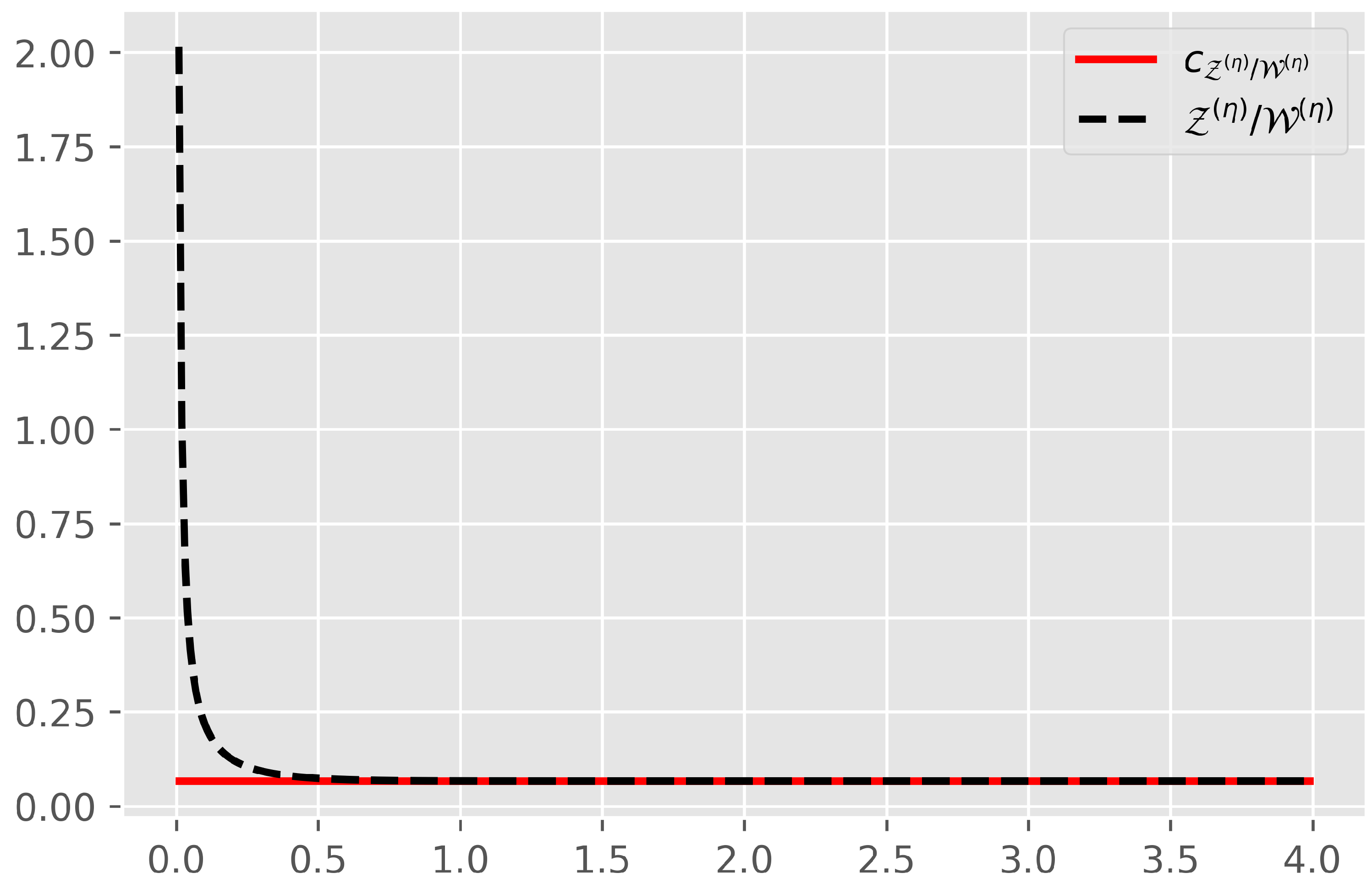
2.4. Theoretical Representation of the Price

The starting point for our entire analysis is the following results. The first one is a corollary from (Al-Hadad and Palmowski 2021, Theorem 15).

Theorem 1.

Let Assumption 1 hold, and assume that ω is non-negative. Then, the optimal stopping region is of the form $(0,u^{*}]$ and we have

1. 

For $\sigma =0$ and $\lambda >0$

$$\begin{array}{cc}\hfill V_{{\mathrm{A}}^{\mathrm{Put}}}^{\omega }(s)& :=\underset{u>0}{sup}{v}_{{\mathrm{A}}^{\mathrm{Put}}}^{\omega }(s,0,u)\hfill \\ & =\underset{u>0}{sup}\left\{\left(K-\frac{u\phi }{\phi +1}\right)\left({\mathcal{Z}}^{({\omega }_u)}\left(\frac{s}{u}\right)-c_{{\mathcal{Z}}^{(\omega )}/{\mathcal{W}}^{(\omega )}}{\mathcal{W}}^{({\omega }_u)}\left(\frac{s}{u}\right)\right)\right\}.\hfill \end{array}$$

(17)

2. 

For $\lambda =0$ and $\sigma >0$

$$\begin{array}{cc}\hfill V_{{\mathrm{A}}^{\mathrm{Put}}}^{\omega }(s)& :=\underset{u>0}{sup}{v}_{{\mathrm{A}}^{\mathrm{Put}}}^{\omega }(s,0,u)\hfill \\ & =\underset{u>0}{sup}\left\{(K-u)\left(\underset{\alpha \to \infty }{lim}{\left(\frac{s}{u}\right)}^{\alpha }\left({\mathcal{Z}}_{\alpha }^{({\omega }_u^{\alpha })}\left(\frac{s}{u}\right)-c_{{\mathcal{Z}}_{\alpha }^{({\omega }^{\alpha })}/{\mathcal{W}}_{\alpha }^{({\omega }^{\alpha })}}{\mathcal{W}}_{\alpha }^{({\omega }_u^{\alpha })}\left(\frac{s}{u}\right)\right)\right)\right\}.\hfill \end{array}$$

(18)

3. 

For $\sigma >0$ and $\lambda >0$

$$\begin{array}{cc}\hfill V_{{\mathrm{A}}^{\mathrm{Put}}}^{\omega }(s)& :=\underset{u>0}{sup}{v}_{{\mathrm{A}}^{\mathrm{Put}}}^{\omega }(s,0,u)\hfill \\ & =\underset{u>0}{sup}\{\left(K-\frac{u\phi }{\phi +1}\right)\left({\mathcal{Z}}^{({\omega }_u)}\left(\frac{s}{u}\right)-c_{{\mathcal{Z}}^{(\omega )}/{\mathcal{W}}^{(\omega )}}{\mathcal{W}}^{({\omega }_u)}\left(\frac{s}{u}\right)\right)\hfill \\ & +(K-u)\left(\underset{\alpha \to \infty }{lim}{\left(\frac{s}{u}\right)}^{\alpha }\left({\mathcal{Z}}_{\alpha }^{({\omega }_u^{\alpha })}\left(\frac{s}{u}\right)-c_{{\mathcal{Z}}_{\alpha }^{({\omega }^{\alpha })}/{\mathcal{W}}_{\alpha }^{({\omega }^{\alpha })}}{\mathcal{W}}_{\alpha }^{({\omega }_u^{\alpha })}\left(\frac{s}{u}\right)\right)\right)\},\hfill \end{array}$$

(19)

where

$$c_{{\mathcal{Z}}^{(\omega )}/{\mathcal{W}}^{(\omega )}}=\underset{z\to \infty }{lim}\frac{{\mathcal{Z}}^{(\omega )}(z)}{{\mathcal{W}}^{(\omega )}(z)}\mathit{and}{c}_{{\mathcal{Z}}_{\alpha }^{({\omega }^{\alpha })}/{\mathcal{W}}_{\alpha }^{({\omega }^{\alpha })}}=\underset{z\to \infty }{lim}\frac{{\mathcal{Z}}_{\alpha }^{({\omega }^{\alpha })}(z)}{{\mathcal{W}}_{\alpha }^{({\omega }^{\alpha })}(z)}.$$

The optimal boundary $u^{*}$ in (18) and (19) can be determined by the smooth fit condition

$${(V_{{\mathrm{A}}^{\mathrm{Put}}}^{\omega })}^{\prime }(u^{*})=-1,$$

while the optimal boundary $u^{*}$ in (17) can be determined by the continuous fit condition

$$V_{{\mathrm{A}}^{\mathrm{Put}}}^{\omega }(u^{*})=K-u^{*}.$$

Remark 1.

Let us note that, using (13) and (14), we can interpret the value functions occurring in Theorem 1 both as the functions of s variable and x variable, where $x=logs$.

Remark 2.

Formula (18) corresponds to the continuous transition of $S_t$ to an interval $(0,u]$, while (17) describes the situation when $S_t$ jumps from $(u,\infty )$ into $(0,u]$. A combination of these two components makes up formula (19).

To find the option price $V_{{\mathrm{A}}^{\mathrm{Put}}}^{\omega }(s)$, we have to identify

$${\mathcal{W}}_{\alpha }^{({\omega }_u^{\alpha })}(s)={\mathcal{W}}_{\alpha }^{({\omega }_u^{\alpha }\circ \exp )}(logs)\mathrm{and}{\mathcal{Z}}_{\alpha }^{({\omega }_u^{\alpha })}(s)={\mathcal{Z}}_{\alpha }^{({\omega }_u^{\alpha }\circ \exp )}(logs),$$

where ${\omega }_u^{\alpha }(s)$ is given in (16), and the case of $\alpha =0$ corresponds to ${\mathcal{W}}^{({\omega }_u)}(s)$ and ${\mathcal{Z}}^{({\omega }_u)}(s)$.

Observe that we need to find the above $\xi$-scale functions for $\xi ={\omega }_u^{\alpha }\circ \exp$ under measure ${\mathbb{P}}^{(\alpha )}$, i.e., we have to identify ${\mathcal{W}}_{\alpha }^{(\xi )}(x)$ and ${\mathcal{Z}}_{\alpha }^{(\xi )}(x)$. This is equivalent to taking our asset price process $S_t$ of the form of (2) but with the new parameters given in (15).

The second key result for our numerical analysis follows straightforward from (Al-Hadad and Palmowski 2021, Theorem 16) and allows us to identify the above omega scale functions using ordinary differential equations.

Theorem 2.

Assume that ξ is continuously differentiable. Then

1. 

If $\sigma =0$ and $\lambda >0$ or $\lambda =0$ and $\sigma >0$, then ${\mathcal{W}}^{(\xi )}(x)$ solves

$${{\mathcal{W}}^{(\xi )}}^{″}(x)=(({\mathsf{{\rm Y}}}_1+{\mathsf{{\rm Y}}}_2)\xi (x)+{\gamma }_2){{\mathcal{W}}^{(\xi )}}^{\prime }(x)+(({\mathsf{{\rm Y}}}_1+{\mathsf{{\rm Y}}}_2){\xi }^{\prime }(x)-{\mathsf{{\rm Y}}}_1{\gamma }_2\xi (x)){\mathcal{W}}^{(\xi )}(x)$$

(20)

with

$$\left\{\begin{array}{c}{\mathcal{W}}^{(\xi )}(0)={\mathsf{{\rm Y}}}_1+{\mathsf{{\rm Y}}}_2,\hfill \\ {{\mathcal{W}}^{(\xi )}}^{\prime }(0)={\mathsf{{\rm Y}}}_2{\gamma }_2+{({\mathsf{{\rm Y}}}_1+{\mathsf{{\rm Y}}}_2)}^2\xi (0).\hfill \end{array}\right.$$

Moreover, ${\mathcal{Z}}^{(\xi )}(x)$ solves the same Equation (20) with

$$\left\{\begin{array}{c}{\mathcal{Z}}^{(\xi )}(0)=1,\hfill \\ {{\mathcal{Z}}^{(\xi )}}^{\prime }(0)=({\mathsf{{\rm Y}}}_1+{\mathsf{{\rm Y}}}_2)\xi (0).\hfill \end{array}\right.$$

2. 

If $\sigma >0$ and $\lambda >0$, then ${\mathcal{W}}^{(\xi )}(x)$ solves

$$\begin{array}{cc}\hfill {{\mathcal{W}}^{(\xi )}}^{‴}(x)& =\left({\gamma }_2+{\gamma }_3\right){{\mathcal{W}}^{(\xi )}}^{″}(x)\hfill \\ & +\left({\mathsf{{\rm Y}}}_2({\gamma }_2-{\gamma }_3)\xi (x)-{\gamma }_2{\gamma }_3-{\mathsf{{\rm Y}}}_1{\gamma }_3\xi (x)\right){{\mathcal{W}}^{(\xi )}}^{\prime }(x)\hfill \\ & +\left({\mathsf{{\rm Y}}}_2({\gamma }_2-{\gamma }_3){\xi }^{\prime }(x)+{\mathsf{{\rm Y}}}_1{\gamma }_2{\gamma }_3\xi (x)-{\mathsf{{\rm Y}}}_1{\gamma }_3{\xi }^{\prime }(x)\right){\mathcal{W}}^{(\xi )}(x)\hfill \end{array}$$

(21)

with

$$\left\{\begin{array}{c}{\mathcal{W}}^{(\xi )}(0)=0,\hfill \\ {{\mathcal{W}}^{(\xi )}}^{\prime }(0)={\mathsf{{\rm Y}}}_2{\gamma }_2+{\mathsf{{\rm Y}}}_3{\gamma }_3,\hfill \\ {{\mathcal{W}}^{(\xi )}}^{″}(0)={\mathsf{{\rm Y}}}_2{{\gamma }_2}^2+{\mathsf{{\rm Y}}}_3{{\gamma }_3}^2.\hfill \end{array}\right.$$

Moreover, ${\mathcal{Z}}^{(\xi )}(x)$ solves the same Equation (21) with

$$\left\{\begin{array}{c}{\mathcal{Z}}^{(\xi )}(0)=1,\hfill \\ {{\mathcal{Z}}^{(\xi )}}^{\prime }(0)=0,\hfill \\ {{\mathcal{Z}}^{(\xi )}}^{″}(0)=\xi (0)({\mathsf{{\rm Y}}}_2({\gamma }_2-{\gamma }_3)-{\mathsf{{\rm Y}}}_1{\gamma }_3).\hfill \end{array}\right.$$

3. Option Pricing—Analytical Approach

In this section, we present some examples of discount functions for which we are able to determine the analytical form of the value function $V_{{\mathrm{A}}^{\mathrm{Put}}}^{\omega }(s)$.

3.1. Constant Discount Function

The case when $\omega$ function is constant, i.e., $\omega (s)=q$ is the standard example which appears in the literature quite extensively. However, this case is quite special, as it turns out that the second term of the sum in (19) simplifies and we do not need to deal with the measure ${\mathbb{P}}^{(\alpha )}$ (and thus to calculate the limit for $\alpha \to \infty$) to find $V_{{\mathrm{A}}^{\mathrm{Put}}}^{\omega }(s)$. This fact is stated in the below theorem.

Theorem 3.

Assume that $\omega (s)=q$. Then

$$\begin{array}{cc}\hfill & \underset{\alpha \to \infty }{lim}{\left(\frac{s}{u}\right)}^{\alpha }\left({\mathcal{Z}}_{\alpha }^{(q-\psi (\alpha ))}\left(\frac{s}{u}\right)-c_{{\mathcal{Z}}_{\alpha }^{(q-\psi (\alpha ))}/{\mathcal{W}}_{\alpha }^{(q-\psi (\alpha ))}}{\mathcal{W}}_{\alpha }^{(q-\psi (\alpha ))}\left(\frac{s}{u}\right)\right)\hfill \\ & =\frac{{\sigma }^2}{2}\left({\mathcal{W}}^{(q)\prime }\left(\frac{s}{u}\right)-\mathsf{\Phi }(q){\mathcal{W}}^{(q)}\left(\frac{s}{u}\right)\right).\hfill \end{array}$$

(22)

Proof. 

Note that

$$\underset{\alpha \to \infty }{lim}{\left(\frac{s}{u}\right)}^{\alpha }\left({\mathcal{Z}}_{\alpha }^{(q-\psi (\alpha ))}\left(\frac{s}{u}\right)-c_{{\mathcal{Z}}_{\alpha }^{(q-\psi (\alpha ))}/{\mathcal{W}}_{\alpha }^{(q-\psi (\alpha ))}}{\mathcal{W}}_{\alpha }^{(q-\psi (\alpha ))}\left(\frac{s}{u}\right)\right)$$

(23)

corresponds to the continuous transition of the process $S_t$ to the interval $(0,u]$ or, in other words, continuous exit from half-line $(u,\infty )$. We define

$${\tau }_b^{+}=inf\{t\ge 0:X_t\ge b\},{\tau }_0^{-}=inf\{t\ge 0:X_t\le 0\}.$$

It turns out that formula (23) is equivalent to

$${\mathbb{E}}_{\frac{s}{u}}\left[e^{-q{\tau }_0^{-}};{\tau }_0^{-}<{\tau }_b^{+},X_{{\tau }_0^{-}}=0\right],$$

for details, see (Al-Hadad and Palmowski 2021, Proof of Theorem 7).

Then, using (Loeffen et al. 2014, (13)) for $x=log\left(\frac{s}{u}\right)$, $a=0$ and $v^{(q)}(x)=W^{(q)\prime }(x)$ together with the fact that $W^{(q)\prime }(0)=\frac{2}{{\sigma }^2}$ (see (Kyprianou 2006, 8.5 (ii), p. 235)), we obtain

$${\mathbb{E}}_{\frac{s}{u}}\left[e^{-q{\tau }_0^{-}};{\tau }_0^{-}<{\tau }_b^{+},X_{{\tau }_0^{-}}=0\right]=\frac{{\sigma }^2}{2}\left(W^{(q)\prime }(x-logu)-\frac{W^{(q)\prime }(b)}{W^{(q)}(b)}{W}^{(q)}(x-logu)\right).$$

Lastly, taking limit $b\uparrow \infty$ and applying L’Hospital’s Rule, complete the proof. □

Ultimately, value function (19) for the constant discount function $\omega (s)=q$ can be written as

$$\begin{array}{cc}\hfill & V_{{\mathrm{A}}^{\mathrm{Put}}}^{\omega }(s)=\underset{u>0}{sup}\{\left(K-\frac{u\phi }{\phi +1}\right)\left({\mathcal{Z}}^{(q)}\left(\frac{s}{u}\right)-c_{{\mathcal{Z}}^{(q)}/{\mathcal{W}}^{(q)}}{\mathcal{W}}^{(q)}\left(\frac{s}{u}\right)\right)\hfill \\ & +(K-u)\frac{{\sigma }^2}{2}\left({\mathcal{W}}^{(q)\prime }\left(\frac{s}{u}\right)-\mathsf{\Phi }(q){\mathcal{W}}^{(q)}\left(\frac{s}{u}\right)\right)\}.\hfill \end{array}$$

Remark 3.

For the case of $\lambda =0$, using (22), one can show that value function (18) simplifies to the well-known formula for the value function in the Black–Scholes model, i.e.,

$$V_{{\mathrm{A}}^{\mathrm{Put}}}^{\omega }(s)=\underset{u>0}{sup}\left((K-u){\left(\frac{s}{u}\right)}^{-\frac{2r}{{\sigma }^2}}\right),$$

where we substituted $q=r$ and $\zeta =r-\frac{{\sigma }^2}{2}$. Therefore, we are not forced to apply the smooth fit condition in order to find the optimal value of u. We can do this analytically by finding the maximum of $V_{{\mathrm{A}}^{\mathrm{Put}}}^{\omega }(s)$ with respect to u.

Figure 1 presents value function (19) for three different values of q, i.e., $q\in \{0.3,0.6,0.9\}$.

Based on Figure 1, we can simply note that a higher value of the discount function $\omega$ results in a smaller value of $V_{{\mathrm{A}}^{\mathrm{Put}}}^{\omega }(s)$, which is in line with the financial intuition.

In turn, Figure 2 shows a comparison of (17)–(19) for the same value of $q=0.5$.

The resulting relation between these functions is again consistent with the economical expectations.

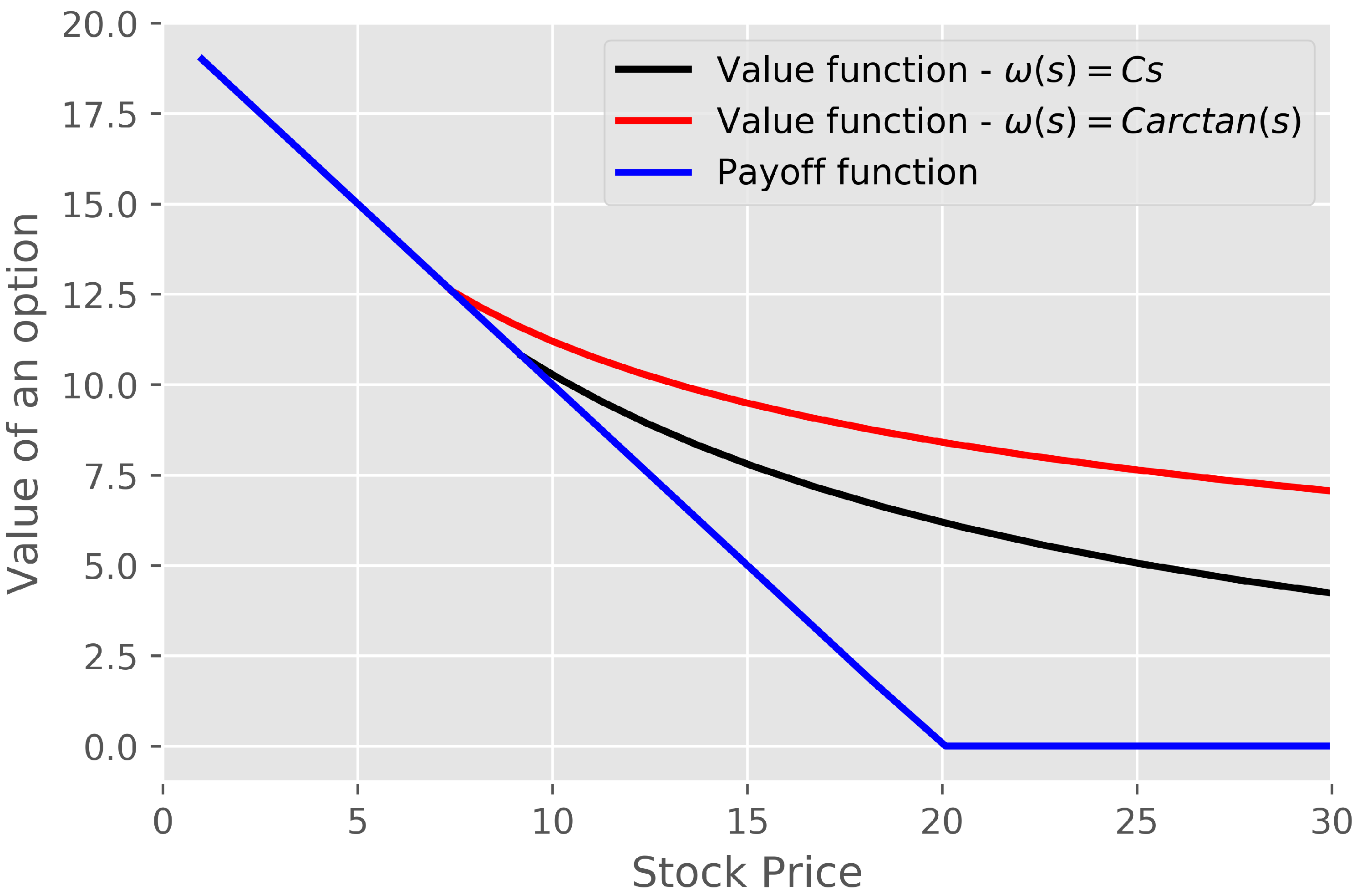
3.2. Linear Discount Function

In this subsection, we consider a linear discount function of the form $\omega (s)=Cs$ for some positive constant C.

3.2.1. $\sigma =0$

Let us consider the case of $\sigma =0$. Then, the asset price process $S_t$ jumps into the interval $(0,u]$, which means from Theorem 1 that

$$V_{{\mathrm{A}}^{\mathrm{Put}}}^{\omega }(s)=\underset{u>0}{sup}\left(K-\frac{u\phi }{\phi +1}\right)\left({\mathcal{Z}}^{({\omega }_u)}\left(\frac{s}{u}\right)-c_{{\mathcal{Z}}^{(\omega )}/{\mathcal{W}}^{(\omega )}}{\mathcal{W}}^{({\omega }_u)}\left(\frac{s}{u}\right)\right),$$

(24)

where ${\omega }_u\left(\frac{s}{u}\right)=\omega (s)=Cs$. Equivalently, (24) can be rewritten as

$$V_{{\mathrm{A}}^{\mathrm{Put}}}^{\eta }(x)=\underset{u>0}{sup}\left(K-\frac{u\phi }{\phi +1}\right)\left({\mathcal{Z}}^{({\eta }_u)}\left(x-logu\right)-c_{{\mathcal{Z}}^{(\eta )}/{\mathcal{W}}^{(\eta )}}{\mathcal{W}}^{({\eta }_u)}\left(x-logu\right)\right),$$

(25)

where $x=logs$ and ${\eta }_u(x-logu)=\eta (x)=C{e}^x$.

To find a closed form of value function (25), we need to identify the scale functions ${\mathcal{W}}^{({\eta }_u)}(x-logu)$ and ${\mathcal{Z}}^{({\eta }_u)}(x-logu)$. From Theorem 2, it follows that both ${\mathcal{W}}^{(\eta )}(x)$ and ${\mathcal{Z}}^{(\eta )}(x)$ solve the following ordinary differential equation

$$f^{″}(x)=(A{e}^x+B)f^{\prime }(x)+D{e}^{x}f(x)$$

(26)

with $A=\frac{C}{\zeta }$, $B=\frac{\lambda -\phi \zeta }{\zeta }$ and $D=C\frac{1+\phi }{\zeta }$, while the initial conditions are as follows

$$\left\{\begin{array}{c}{\mathcal{W}}^{(\eta )}(0)=\frac{1}{\zeta },\hfill \\ {{\mathcal{W}}^{(\eta )}}^{\prime }(0)=\frac{C+\lambda }{{\zeta }^2}\hfill \end{array}\right.$$

(27)

and

$$\left\{\begin{array}{c}{\mathcal{Z}}^{(\eta )}(0)=1,\hfill \\ {{\mathcal{Z}}^{(\eta )}}^{\prime }(0)=\frac{C}{\zeta }.\hfill \end{array}\right.$$

(28)

Substituting $t=A{e}^x$ and $F(t)=f(x)$ to (26), we obtain the Kummer’s equation of the form

$$t{F}^{″}(t)+(b-t)F^{\prime }(t)-aF(t)=0,$$

(29)

where $b=1-B$ and $a=\frac{D}{A}$.

If b is not an integer, then the general solution to (29) has the form

$$F(t)=K_1{}_1{F}_1(a_1,b_1;t)+K_2{t}^{1-b}{}_1{F}_1(a_2,b_2;t),$$

(30)

where $K_1$ and $K_2$ are the constants that can be found based on the initial conditions, $a_1=a$, $b_1=b$, $a_2=a-b+1$, $b_2=2-b$, while ${}_1{F}_1(·,·;·)$ is the Kummer confluent hypergeometric function.

We denote by $K_1^W$, $K_2^W$ and $K_1^Z$, $K_2^Z$ the constants corresponding to ${\mathcal{W}}^{(\eta )}(x)$ and ${\mathcal{Z}}^{(\eta )}(x)$, respectively. Using initial conditions (27) and (28), we can simply calculate these constants for both ${\mathcal{W}}^{(\eta )}(x)$ and ${\mathcal{Z}}^{(\eta )}(x)$. By shifting these functions by $logu$, we simply produce ${\mathcal{W}}^{({\eta }_u)}(x-logu)$ and ${\mathcal{Z}}^{({\eta }_u)}(x-logu)$.

The asymptotic behaviour of ${}_1{F}_1\left(a,b;t\right)$ for $t\to \infty$ is as follows

$${}_1{F}_1(a,b;t)=\frac{\mathsf{\Gamma }(b)}{\mathsf{\Gamma }(a)}{e}^t{t}^{a-b}\left[1+O\left(\frac{1}{t}\right)\right].$$

(31)

Based on (31), we calculate the constant $c_{{\mathcal{Z}}^{(\eta )}/{\mathcal{W}}^{(\eta )}}$ (or equivalenly $c_{{\mathcal{Z}}^{(\omega )}/{\mathcal{W}}^{(\omega )}}$) occuring in (25). It has the following form

$$c_{{\mathcal{Z}}^{(\eta )}/{\mathcal{W}}^{(\eta )}}=\frac{K_1^Z\frac{\mathsf{\Gamma }(b_1)}{\mathsf{\Gamma }(a_1)}{A}^{a_1-b_1}+K_2^Z\frac{\mathsf{\Gamma }(b_2)}{\mathsf{\Gamma }(a_2)}{A}^{a_2-1}}{K_1^W\frac{\mathsf{\Gamma }(b_1)}{\mathsf{\Gamma }(a_1)}{A}^{a_1-b_1}+K_2^W\frac{\mathsf{\Gamma }(b_2)}{\mathsf{\Gamma }(a_2)}{A}^{a_2-1}}.$$

(32)

Combining all the obtained results and substituting them into (25), we can present value function (25) graphically for some sample parameter values. This is carried out in Section 4.

3.2.2. $\lambda =0$

Let us consider the case of $\lambda =0$. In this case, the asset price process $S_t$ enters the interval $(0,u]$ in a continuous way only. Therefore, from Theorem 1

$$\begin{array}{c}\hfill V_{{\mathrm{A}}^{\mathrm{Put}}}^{\omega }(s)=\underset{u>0}{sup}\left\{(K-u)\left(\underset{\alpha \to \infty }{lim}{\left(\frac{s}{u}\right)}^{\alpha }\left({\mathcal{Z}}_{\alpha }^{({\omega }_u^{\alpha })}\left(\frac{s}{u}\right)-c_{{\mathcal{Z}}_{\alpha }^{({\omega }^{\alpha })}/{\mathcal{W}}_{\alpha }^{({\omega }^{\alpha })}}{\mathcal{W}}_{\alpha }^{({\omega }_u^{\alpha })}\left(\frac{s}{u}\right)\right)\right)\right\}\end{array}$$

(33)

which is equivalent to

$$V_{{\mathrm{A}}^{\mathrm{Put}}}^{\eta }(x)=\underset{u>0}{sup}\left\{(K-u)\left(\underset{\alpha \to \infty }{lim}{e}^{\alpha (x-logu)}\left({\mathcal{Z}}_{\alpha }^{({\eta }_u^{\alpha })}(x-logu)-c_{{\mathcal{Z}}_{\alpha }^{({\eta }^{\alpha })}/{\mathcal{W}}_{\alpha }^{({\eta }^{\alpha })}}{\mathcal{W}}_{\alpha }^{({\eta }_u^{\alpha })}(x-logu)\right)\right)\right\}.$$

(34)

It suffices to find now ${\mathcal{W}}_{\alpha }^{({\eta }_u^{\alpha })}(x-logu)$ and ${\mathcal{Z}}_{\alpha }^{({\eta }_u^{\alpha })}(x-logu)$. From Theorem 2, it follows that ${\mathcal{W}}_{\alpha }^{({\eta }^{\alpha })}(x)$ and ${\mathcal{Z}}_{\alpha }^{({\eta }^{\alpha })}(x)$ solve

$$f^{″}(x)=B_{\alpha }{f}^{\prime }(x)+(D_{\alpha }{e}^x+E_{\alpha })f(x)$$

(35)

with $B_{\alpha }=-\frac{2}{{\sigma }^2}(\zeta +{\sigma }^2\alpha )$, $D_{\alpha }=\frac{2C}{{\sigma }^2}$ and $E_{\alpha }=-\frac{2}{{\sigma }^2}\left(\zeta \alpha +\frac{{\sigma }^2}{2}{\alpha }^2\right)$. The initial conditions have the following form

$$\left\{\begin{array}{c}{\mathcal{W}}_{\alpha }^{({\eta }^{\alpha })}(0)=0,\hfill \\ {{\mathcal{W}}_{\alpha }^{({\eta }^{\alpha })}}^{\prime }(0)=\frac{2}{{\sigma }^2}\hfill \end{array}\right.$$

(36)

and

$$\left\{\begin{array}{c}{\mathcal{Z}}_{\alpha }^{({\eta }_u^{\alpha })}(0)=1,\hfill \\ {{\mathcal{Z}}_{\alpha }^{({\eta }_u^{\alpha })}}^{\prime }(0)=0.\hfill \end{array}\right.$$

(37)

Substituting $t=2\sqrt{-D_{\alpha }{e}^x}$ and $F(t)=e^{-\frac{B_{\alpha }x}{2}}f(x)$ to (35), we obtain the Bessel differential equation of the form

$$t^2{F}^{″}(t)+t{F}^{\prime }(t)+(t^2-v^2)F(t)=0,$$

(38)

where $v=\sqrt{{B_{\alpha }}^2+4E_{\alpha }}=\frac{2\zeta }{{\sigma }^2}$. The general solution to (38) is equal to

$$F(t)=K_1{J}_v(t)+K_2{Y}_v(t)$$

and therefore

$$f(x)=e^{\frac{B_{\alpha }x}{2}}\left(K_1{J}_v(2\sqrt{-D_{\alpha }{e}^x})+K_2{Y}_v(2\sqrt{-D_{\alpha }{e}^x})\right).$$

(39)

Based on the form of (39) and the fact that $D_{\alpha }$ does not depend on $\alpha$, we can simply note that value function (34) is also independent of $\alpha$. Therefore, we can take an arbitrary value of $\alpha$ in (35). Thanks to this key observation, its solution (39) can take a simplified form. Indeed, for $\alpha =0$, Equation (35) is equal to

$$f^{″}(x)=B_0{f}^{\prime }(x)+D_0{e}^{x}f(x),$$

(40)

where $B_0=\frac{-2\zeta }{{\sigma }^2}$ and $D_0=\frac{2C}{{\sigma }^2}$. Hence, the general solution to (40) takes the following form

$$f(x)=e^{\frac{B_{0}x}{2}}\left(K_1{J}_v(2\sqrt{-D_0{e}^x})+K_2{Y}_v(2\sqrt{-D_0{e}^x})\right).$$

(41)

For $B_0=\frac{1}{2}-n$, where $n\in {\mathbb{N}}_0$ and $D_{0}t>0$, Equation (41) reduces to

$$f(x)=K_1{\left(cosh\left(4\sqrt{D_0{e}^x}\right)\right)}^n+K_2{\left(sinh\left(4\sqrt{D_0{e}^x}\right)\right)}^n.$$

If we take the following sample parameters $r=0.05$ and $\sigma =0.2$, we obtain $n=2$ and therefore

$$\begin{array}{cc}\hfill f(x)& =K_1\left(\frac{3sinh(2\sqrt{e^x})}{4e^{\frac{5}{2}x}}+\frac{sinh(2\sqrt{e^x})}{e^{\frac{3}{2}x}}-\frac{3cosh(2\sqrt{e^x})}{2e^{2x}}\right)\hfill \\ & +K_2\left(\frac{3cosh(2\sqrt{e^x})}{4e^{\frac{5}{2}x}}+\frac{cosh(2\sqrt{e^x})}{e^{\frac{3}{2}x}}-\frac{3sinh(2\sqrt{e^x})}{2e^{2x}}\right).\hfill \end{array}$$

(42)

Applying initial conditions (36) and (37), we can simply obtain $K_1^W$, $K_2^W$ and $K_1^Z$, $K_2^Z$. Using equality (42), which holds for both ${\mathcal{W}}_{\alpha }^{({\eta }^{\alpha })}(x)$ and ${\mathcal{Z}}_{\alpha }^{({\eta }^{\alpha })}(x)$, we can calculate that

$$\begin{array}{c}\hfill c_{{\mathcal{Z}}_{\alpha }^{({\eta }^{\alpha })}/{\mathcal{W}}_{\alpha }^{({\eta }^{\alpha })}}=c_{{\mathcal{Z}}^{(\eta )}/{\mathcal{W}}^{(\eta )}}=\frac{K_1^Z+K_2^Z}{K_1^W+K_2^W}.\end{array}$$

(43)

Taking into account all the obtained results, we can obtain value function (34) for sample data. This is performed in Section 4 as well.

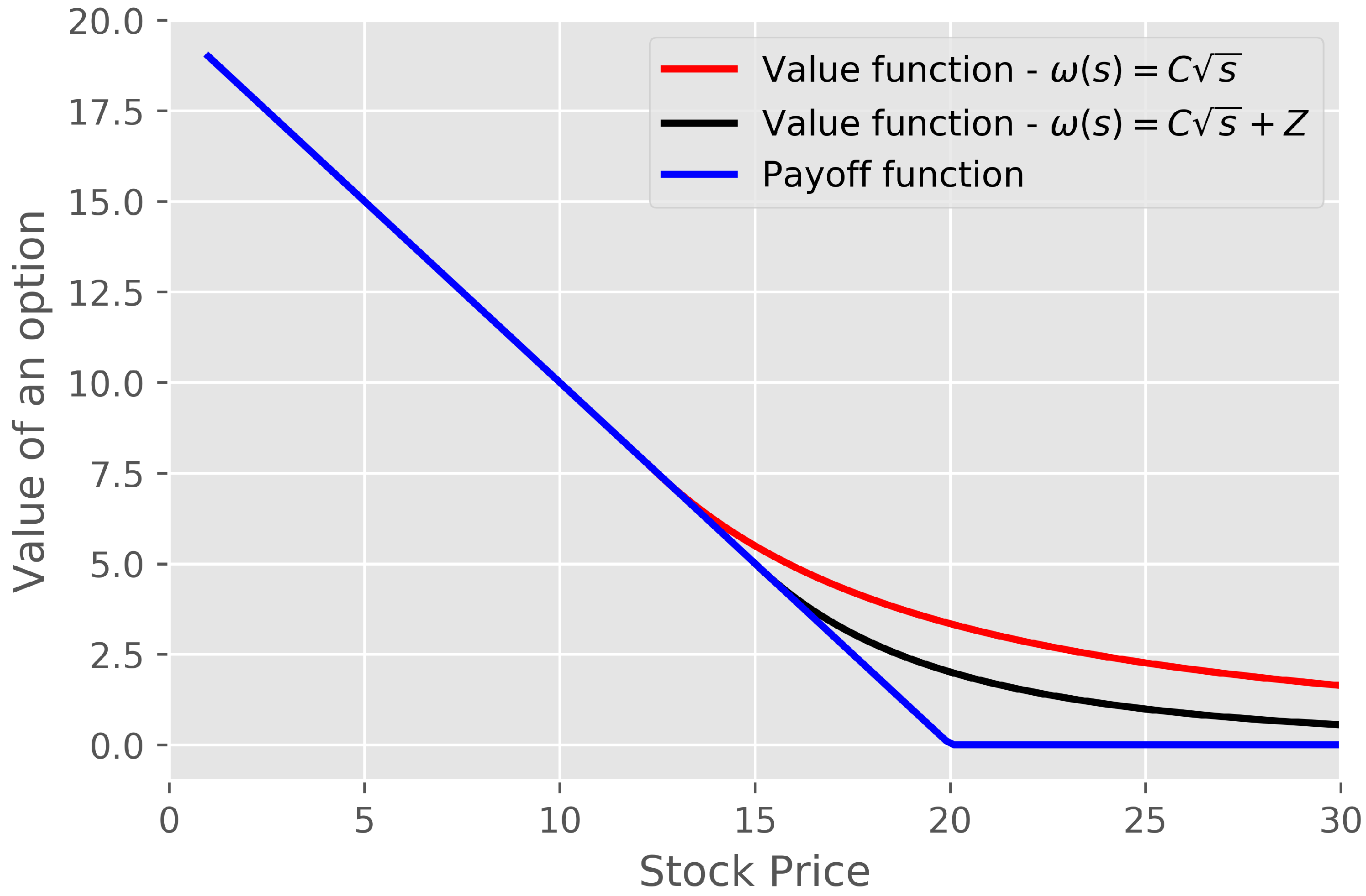
3.3. Power Discount Function

This time, we take into account a power function of the form $\omega (s)=C{s}^n$ for $n\in (0,1]$ and C being some positive contant. This case is a generalisation of a linear discount function.

3.3.1. $\sigma =0$

Similar to the case of a linear discount function, the scale functions ${\mathcal{W}}^{(\eta )}(x)$ and ${\mathcal{Z}}^{(\eta )}(x)$ solve

$$f^{″}(x)=(A{e}^{nx}+B)f^{\prime }(x)+D{e}^{nx}f(x)$$

(44)

with $A=\frac{C}{\zeta }$, $B=\frac{\lambda -\phi \zeta }{\zeta }$ and $D=C\frac{n+\phi }{\zeta }$, while the initial conditions are the same as those provided in (27) and (28). Applying a substitution $t=\frac{A}{n}{e}^{nx}$ and $F(t)=f(x)$, we transform (44) into

$$t{F}^{″}(t)+(b-t)F^{\prime }(t)-aF(t)=0,$$

(45)

where $b=1-\frac{B}{n}$ and $a=\frac{D}{An}$. The general solution to (45) has the same form as was provided in (30).

Therefore, for both the linear and the power discount function $\omega$, the form of the value function $V_{{\mathrm{A}}^{\mathrm{Put}}}^{\eta }(x)$ is identical.

3.3.2. $\lambda =0$

As in the above case, the idea of finding a closed form of the value function can be borrowed from the linear case. This time, the scale functions ${\mathcal{W}}_{\alpha }^{({\eta }^{\alpha })}(x)$ and ${\mathcal{Z}}_{\alpha }^{({\eta }^{\alpha })}(x)$ satisfy the equation

$$f^{″}(x)=B_{\alpha }{f}^{\prime }(x)+(D_{\alpha }{e}^{nx}+E_{\alpha })f(x)$$

with $B_{\alpha }=-\frac{2}{{\sigma }^2}(\zeta +{\sigma }^2\alpha )$, $D_{\alpha }=\frac{2C}{{\sigma }^2}$ and $E_{\alpha }=-\frac{2}{{\sigma }^2}\left(\zeta \alpha +\frac{{\sigma }^2}{2}{\alpha }^2\right)$, while the initial conditions are of the form (36) and (37). If we substitute $t=\frac{2}{n}\sqrt{-D_{\alpha }{e}^{nx}}$ and $F(t)=e^{-\frac{B_{\alpha }x}{2}}f(x)$, we receive the Bessel differential equation for $F(t)$ with the solution

$$F(t)=K_1{J}_v(t)+K_2{Y}_v(t).$$

Therefore, we have

$$f(x)=e^{\frac{B_{\alpha }x}{2}}\left(K_1{J}_v\left(\frac{2}{n}\sqrt{-D_{\alpha }{e}^{nx}}\right)+K_2{Y}_v\left(\frac{2}{n}\sqrt{-D_{\alpha }{e}^{nx}}\right)\right),$$

(46)

where $v=\frac{\sqrt{{B_{\alpha }}^2+4E_{\alpha }}}{n}=\frac{2\zeta }{n{\sigma }^2}$. We can show, as in the prevoius section, that the value function which arises in this scenario does not depend on $\alpha$. Thus, for $\alpha =0$, (46) takes the form

$$f(x)=e^{\frac{B_{0}x}{2}}\left(K_1{J}_v\left(\frac{2}{n}\sqrt{-D_0{e}^{nx}}\right)+K_2{Y}_v\left(\frac{2}{n}\sqrt{-D_0{e}^{nx}}\right)\right).$$

Again, having exact formulas for the scale functions, we can easily represent the form of the value function. All results are presented in Section 4.

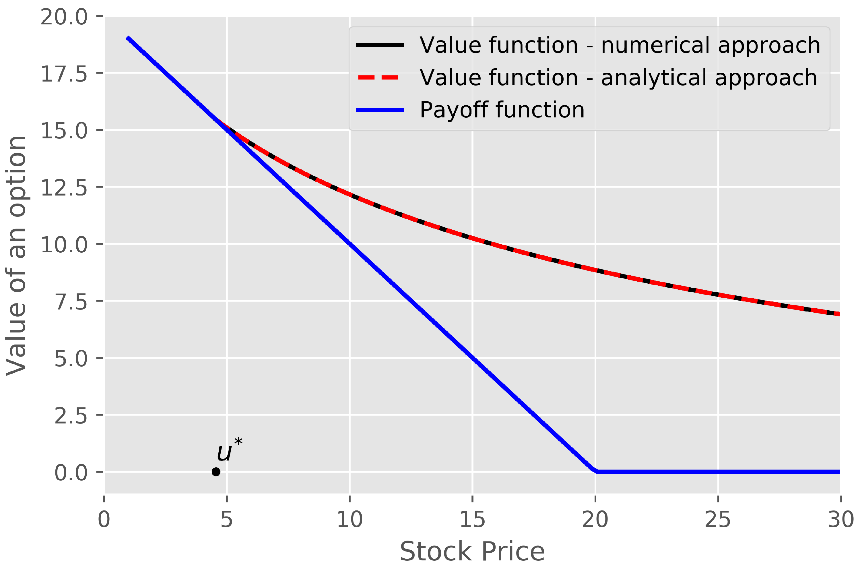
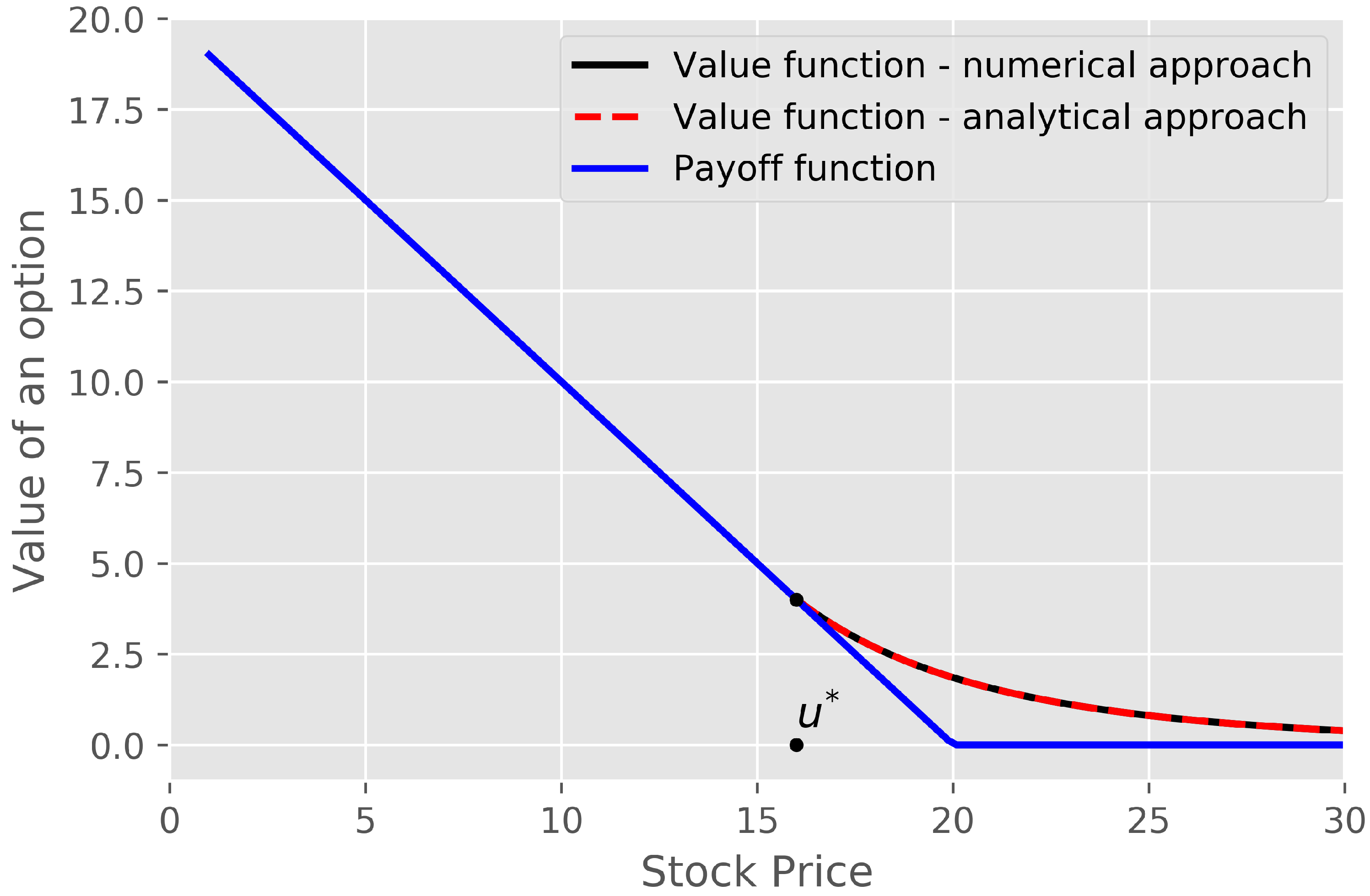
4. Option Pricing—Numerical Approach

In this section, we show how to numerically identify the value function $V_{{\mathrm{A}}^{\mathrm{Put}}}^{\omega }(s)$ for arbitrary discount function $\omega$. We present some figures corresponding to the various discount functions as well.

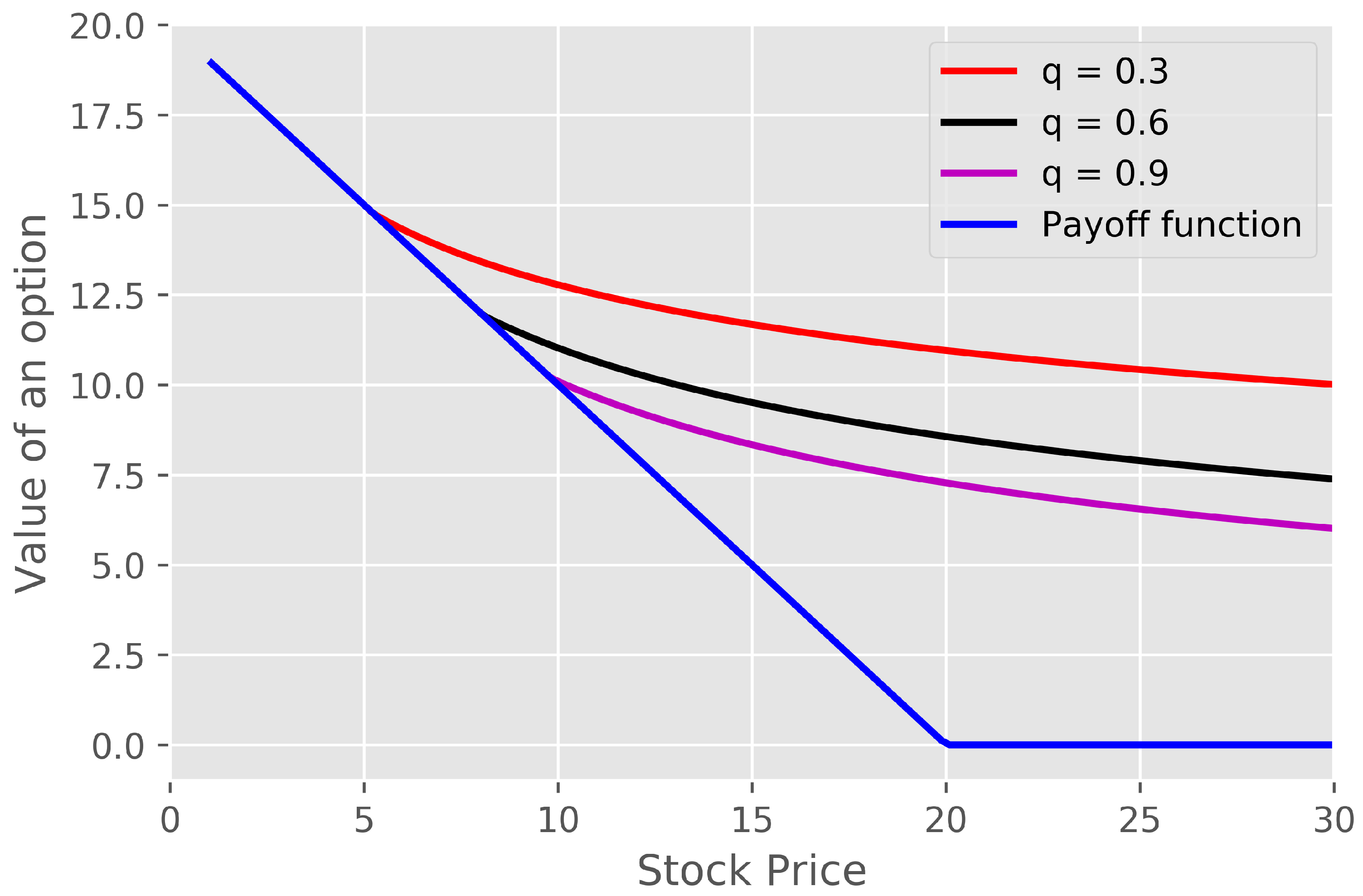
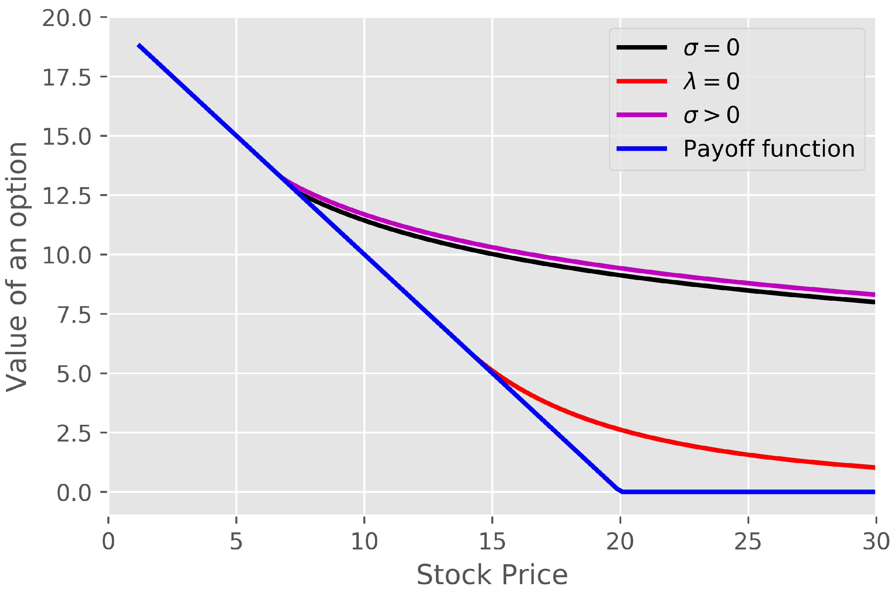
4.1. Different Discount Functions

For some discount functions $\omega$, we are unable to find the analytical forms of ${\mathcal{W}}^{(\eta )}(x)$, ${\mathcal{Z}}^{(\eta )}(x)$, ${\mathcal{W}}_{\alpha }^{({\eta }^{\alpha })}(x)$ and ${\mathcal{Z}}_{\alpha }^{({\eta }^{\alpha })}(x)$, which are the solutions to the ordinary differential equations occurring in Theorem 2. That is, formally we cannot identify explicitly the value function either. In such a situation, we can proceed a numerical analysis of these equations.

In general, solving a high-order ordinary differential equation consists of transforming it into first-order vector form and then applying an appropriate algorithm that returns the numerical solution of the $n+1$-dimensional system of first-order ordinary differential equations. For practical purposes, however—such as in financial engineering—numeric approximations to the solutions of ordinary differential equations are often sufficient. In this paper, we focus on the Higher-Order Taylor Method. This method employs the Taylor polynomial of the solution to the equation. It approximates the 0-th order term by using the previous step’s value (which is the initial condition for the first step), and the subsequent terms of the Taylor expansion by using the differential equation.

4.1.1. $\sigma =0$

For the case of $\sigma =0$, we showed in the previous section how to derive the value function for the linear discount function $\omega$. Figure 3 presents comparison of the value function given in (24) when the scale functions were calculated analytically (as shown in Section 3.2.1) and numerically by solving differential ordinary Equation (26). In this example, a linear discount function was chosen, i.e., $\omega (s)=Cs$. The difference between these functions is so small that this is negligible.

Moreover, Figure 4 illustrates the constant $c_{{\mathcal{Z}}^{(\eta )}/{\mathcal{W}}^{(\eta )}}$ obtained in (32) together with the quotient of the functions ${\mathcal{Z}}^{(\eta )}(x)$ and ${\mathcal{W}}^{(\eta )}(x)$.

As we mentioned at the beginning of this section, we are not always able to get an analytical solution to an ordinary differential equation. This is the case, for example, when the discount function is of the form $\omega (s)=Carctan(s)$ for some positive C. Then, we can only obtain the scale functions numerically. Figure 5 shows two value functions, for $\omega (s)=Cs$ and $\omega (s)=Carctan(s)$, respectively. Since for all positive s we have $s>arctan(s)$, then we expect that the value function corresponding to $\omega (s)=Carctan(s)$ takes greater values rather than for $\omega (s)=Cs$. We can also note that the difference between these functions becomes greater for higher values of s, which is in line with economical intuition since the difference between $\omega (s)=s$ and $\omega (s)=arctan(s)$ also extends as s increases.

4.1.2. $\lambda =0$

The case of $\lambda =0$ corresponds to the situation when the stock price process (2) does not have any jumps. Then, the value function takes the form (18). From the numerical point of view, the problem lies in choosing a sufficiently large value of $\alpha$ in (18) to obtain the final and right form of the value function. In this section, we avoid this problem by selecting discount functions for which the value function is independent of the $\alpha$ parameter.

Figure 6 presents a comparison of the value function given in (33) for $\omega (s)=Cs$ and for the scale functions obtained analytically and numerically. As shown in Section 3.2.2, in this case, we can take an arbitrary value of $\alpha$ and obtain a simplified form of the value function and ordinary differential equation that the scale functions solve. Similar to the previous example, we again can observe a negligible difference between these two value functions.

In turn, Figure 7 shows the constant $c_{{\mathcal{Z}}^{(\eta )}/{\mathcal{W}}^{(\eta )}}$ given in (43) with the ratio of ${\mathcal{Z}}^{(\eta )}(x)$ and ${\mathcal{W}}^{(\eta )}(x)$.

Lastly, in Figure 8, we can observe the value functions for both $\omega (s)=C\sqrt{s}$ and $\omega (s)=C\sqrt{s}+Z$ for some positive Z, i.e., we compare two discount functions that differ in shift. This time, we can see that the value functions obtained in this way also differ only in shift, which confirms financial intuition.

4.1.3. $\sigma >0$ and $\lambda >0$

The most general case is when $\sigma >0$ and $\lambda >0$. Then, the considered value function $V_{{\mathrm{A}}^{\mathrm{Put}}}^{\omega }(s)$ is given by (19). It can be also represented as the function of x variable:

$$\begin{array}{cc}\hfill & V_{{\mathrm{A}}^{\mathrm{Put}}}^{\eta }(x)=\underset{u>0}{sup}\{\left(K-\frac{u\phi }{\phi +1}\right)\left({\mathcal{Z}}^{({\eta }_u)}(x-logu)-c_{{\mathcal{Z}}^{(\eta )}/{\mathcal{W}}^{(\eta )}}{\mathcal{W}}^{({\eta }_u)}(x-logu)\right)\hfill \\ & +(K-u)\left(\underset{\alpha \to \infty }{lim}{e}^{\alpha (x-logu)}\left({\mathcal{Z}}_{\alpha }^{({\eta }_u^{\alpha })}(x-logu)-c_{{\mathcal{Z}}_{\alpha }^{({\eta }^{\alpha })}/{\mathcal{W}}_{\alpha }^{({\eta }^{\alpha })}}{\mathcal{W}}_{\alpha }^{({\eta }_u^{\alpha })}(x-logu)\right)\right)\}.\hfill \end{array}$$

(47)

For the linear discount function $\omega (s)=Cs$, the scale functions ${\mathcal{W}}^{(\eta )}(x)$ and ${\mathcal{Z}}^{(\eta )}(x)$ occurring in (47) are the solutions to the following ordinary differential equation

$$\begin{array}{cc}\hfill f^{‴}(x)& =A{f}^{″}(x)+(B{e}^x+D)f^{\prime }(x)+E{e}^{x}f(x)\hfill \end{array}$$

(48)

with $A={\gamma }_2+{\gamma }_3$, $B=C\left[{\mathsf{{\rm Y}}}_2({\gamma }_2-{\gamma }_3)-{\mathsf{{\rm Y}}}_1{\gamma }_3\right]$, $D=-{\gamma }_2{\gamma }_3$, $E=C[{\mathsf{{\rm Y}}}_2({\gamma }_2-{\gamma }_3)$ $+{\mathsf{{\rm Y}}}_1{\gamma }_2{\gamma }_3-{\mathsf{{\rm Y}}}_1{\gamma }_3]$.

The initial conditions for ${\mathcal{W}}^{(\eta )}(x)$ and ${\mathcal{Z}}^{(\eta )}(x)$ are as follows

$$\left\{\begin{array}{c}{\mathcal{W}}^{(\eta )}(0)=0,\hfill \\ {{\mathcal{W}}^{(\eta )}}^{\prime }(0)={\mathsf{{\rm Y}}}_2{\gamma }_2+{\mathsf{{\rm Y}}}_3{\gamma }_3,\hfill \\ {{\mathcal{W}}^{(\eta )}}^{″}(0)={\mathsf{{\rm Y}}}_2{{\gamma }_2}^2+{\mathsf{{\rm Y}}}_3{{\gamma }_3}^2\hfill \end{array}\right.$$

and

$$\left\{\begin{array}{c}{\mathcal{Z}}^{(\eta )}(0)=1,\hfill \\ {{\mathcal{Z}}^{(\eta )}}^{\prime }(0)=0,\hfill \\ {{\mathcal{Z}}^{(\eta )}}^{″}(0)=C\left[{\mathsf{{\rm Y}}}_2({\gamma }_2-{\gamma }_3)-{\mathsf{{\rm Y}}}_1{\gamma }_3\right].\hfill \end{array}\right.$$

Thus, ${\mathcal{W}}_{\alpha }^{({\eta }^{\alpha })}(x)$ and ${\mathcal{Z}}_{\alpha }^{({\eta }^{\alpha })}(x)$ solve

$$\begin{array}{cc}\hfill f^{‴}(x)& =A_{\alpha }{f}^{″}(x)+(B_{\alpha }{e}^x+D_{\alpha })f^{\prime }(x)+(E_{\alpha }{e}^x+F_{\alpha })f(x)\hfill \end{array}$$

(49)

with $A_{\alpha }={\gamma }_{{\alpha }_2}+{\gamma }_{{\alpha }_3}$, $B_{\alpha }=C\left[{\mathsf{{\rm Y}}}_{{\alpha }_2}({\gamma }_{{\alpha }_2}-{\gamma }_{{\alpha }_3})-{\mathsf{{\rm Y}}}_{{\alpha }_1}{\gamma }_{{\alpha }_3}\right]$, $D_{\alpha }=-{\mathsf{{\rm Y}}}_{{\alpha }_2}({\gamma }_{{\alpha }_2}-{\gamma }_{{\alpha }_3})\psi (\alpha )-{\gamma }_2{\gamma }_3+{\mathsf{{\rm Y}}}_{{\alpha }_1}{\gamma }_{{\alpha }_3}\psi (\alpha )$, $E_{\alpha }=C\left[{\mathsf{{\rm Y}}}_{{\alpha }_2}({\gamma }_{{\alpha }_2}-{\gamma }_{{\alpha }_3})+{\mathsf{{\rm Y}}}_{{\alpha }_1}{\gamma }_{{\alpha }_2}{\gamma }_{{\alpha }_3}-{\mathsf{{\rm Y}}}_{{\alpha }_1}{\gamma }_{{\alpha }_3}\right]$, $F_{\alpha }=-{\mathsf{{\rm Y}}}_{{\alpha }_1}{\gamma }_{{\alpha }_2}{\gamma }_{{\alpha }_3}\psi (\alpha )$. The initial conditions for ${\mathcal{W}}_{\alpha }^{({\eta }^{\alpha })}(x)$ and ${\mathcal{Z}}_{\alpha }^{({\eta }^{\alpha })}(x)$ are as follows

$$\left\{\begin{array}{c}{\mathcal{W}}_{\alpha }^{({\eta }^{\alpha })}(0)=0,\hfill \\ {{\mathcal{W}}_{\alpha }^{({\eta }^{\alpha })}}^{\prime }(0)={\mathsf{{\rm Y}}}_{{\alpha }_2}{\gamma }_{{\alpha }_2}+{\mathsf{{\rm Y}}}_{{\alpha }_3}{\gamma }_{{\alpha }_3},\hfill \\ {{\mathcal{W}}_{\alpha }^{({\eta }^{\alpha })}}^{″}(0)={\mathsf{{\rm Y}}}_{{\alpha }_2}{{\gamma }_{{\alpha }_2}}^2+{\mathsf{{\rm Y}}}_{{\alpha }_3}{{\gamma }_{{\alpha }_3}}^2\hfill \end{array}\right.$$

and

$$\left\{\begin{array}{c}{\mathcal{Z}}_{\alpha }^{({\eta }^{\alpha })}(0)=1,\hfill \\ {{\mathcal{Z}}_{\alpha }^{({\eta }^{\alpha })}}^{\prime }(0)=0,\hfill \\ {{\mathcal{Z}}_{\alpha }^{({\eta }^{\alpha })}}^{″}(0)=C\left[{\mathsf{{\rm Y}}}_{{\alpha }_2}({\gamma }_{{\alpha }_2}-{\gamma }_{{\alpha }_3})-{\mathsf{{\rm Y}}}_{{\alpha }_1}{\gamma }_{{\alpha }_3}\right].\hfill \end{array}\right.$$

In this case, we are not able to identify explicit solutions to third-order ordinary differential Equations (48) and (49). Therefore, we are forced to use only the numerical method to find the scale functions and, hence, the value function.

Figure 9 shows several graphs of the value function (19) for different values of $\alpha$ parameter together with the first and second component occurring in (19).

5. Conclusions

In this paper, we have presented a novel approach to pricing the perpetual American put options with asset-dependent discounting. For the asset price process $S_t$ being the geometric spectrally negative Lévy process, we have shown that the value function (1) is the solution of the ordinary differential equations given in Theorem 2. We have used these theoretical results to perform extended numerical analysis for some key financial examples. In particular, for some cases, we have managed to produce some explicit formulas for the value function. In the cases where it was impossible to do so, we have used the numerical analysis of the above-mentioned ordinary differential equations based on the Higher-Order Taylor Method. We have presented many figures of the value functions that arise in various scenarios.

One can think of further generalisations; for example, when the discount factor is randomised. Thia can be achieved in different ways, e.g., by introducing additional Markov economical environment. One can also think about other very realistic models for financial assets, for example, based on generalised hyperbolic distributions and their subclasses; see Prause (1999), for more details. This type of research is left for future investigations.

References

1. Al-Hadad, Jonas, and Zbigniew Palmowski. 2021. Perpetual American Options with Asset-Dependent Discounting. Submitted for Publication. Available online: https://arxiv.org/abs/2007.09419 (accessed on 18 July 2020).
2. Cohen, Serge, Alexey Kuznetsov, Andreas Kyprianou, and Victor Rivero. 2013. Lévy Matters II. Berlin/Heidelberg: Springer. [Google Scholar]
3. Cont, Rama, and Peter Tankov. 2004. Financial Modelling with Jump Processes. Boca Raton: Chapman & Hall. [Google Scholar]
4. De Donno, Marzia, Zbigniew Palmowski, and Joanna Tumilewicz. 2020. Double continuation regions for American and Swing options with negative discount rate in Lévy models. Mathematical Finance 30: 196–227. [Google Scholar] [CrossRef] [Green Version]
5. Kou, Steven G. 2002. A Jump-Diffusion Model for Option Pricing. Management Science 48: 1086–1101. [Google Scholar] [CrossRef] [Green Version]
6. Kyprianou, Andreas E. 2006. Introductory Lectures on Fluctuations of Lévy Processes with Applications. Berlin/Heidelberg: Springer. [Google Scholar]
7. Li, Bo, and Zbigniew Palmowski. 2018. Fluctuations of omega–killed spectrally negative Lévy processes. Stochastic Processes and their Applications 128: 3273–99. [Google Scholar] [CrossRef] [Green Version]
8. Linetsky, Vadim. 1999. Step options. Mathematical Finance 9: 55–96. [Google Scholar] [CrossRef]
9. Loeffen, Ronnie L., Jean-François Renaud, and Xiaowen Zhou. 2014. Occupation times of intervals until first passage times for spectrally negative Lévy processes. Stochastic Processes and their Applications 124: 1408–143. [Google Scholar] [CrossRef] [Green Version]
10. Palmowski, Zbigniew, and Tomasz Rolski. 2002. A technique for exponential change of measure for Markov processes. Bernoulli 8: 767–85. [Google Scholar]
11. Peskir, Goran, and Albert Shiryaev. 2006. Optimal Stopping and Free–Boundary Problems. Basel: Birkhäuser. [Google Scholar]
12. Prause, Karsten. 1999. The Generalized Hyperbolic Model: Estimation, Financial Derivatives, and Risk Measures. Ph.D. thesis, University of Freiburg, Breisgau, Germany. Available online: https://d-nb.info/961152192/34 (accessed on October 1999).
13. Rodosthenous, Neofytos, and Hongzhong Zhang. 2018. Beating the omega clock: An optimal stopping problem with random time-horizon under spectrally negative Lévy models. Annals of Applied Probability 28: 2105–40. [Google Scholar] [CrossRef]
Figure 1. The value and payoff functions for the given set of parameters: K = 20 , r = 0.05 , σ = 0.2 , λ = 6 , φ = 2 and q { 0.3 , 0.6 , 0.9 } .
Jrfm 14 00130 g001
Figure 2. The value and payoff functions for the given set of parameters: K = 20 , r = 0.05 , σ = 0.4 , λ = 6 , φ = 2 and q = 0.5 .
Jrfm 14 00130 g002
Figure 3. Comparison of value function (24) for ω ( s ) = C s for both methods of determining the scale functions—analytical and numerical one. The chosen set of parameters is as follows: K = 20 , C = 0.1 , r = 0.05 , λ = 6 , φ = 2 .
Jrfm 14 00130 g003
Figure 4. Comparison of the constant c Z ( η ) / W ( η ) and the ratio of Z ( η ) ( x ) and W ( η ) ( x ) for a linear discount function ω ( s ) = C s and K = 20 , C = 0.1 , r = 0.05 , λ = 6 , φ = 2 .
Jrfm 14 00130 g004
Figure 5. Comparison of value function (24) for both ω ( s ) = C s and ω = C arctan ( s ) and for the given set of parameters: K = 20 , C = 0.5 , r = 0.05 , λ = 6 , φ = 2 .
Jrfm 14 00130 g005
Figure 6. Comparison of value function (33) for ω ( s ) = C s for both methods of determining the scale functions–analytical and numerical one. The chosen set of parameters is as follows: K = 20 , C = 0.1 , r = 0.05 , σ = 0.2 .
Jrfm 14 00130 g006
Figure 7. Comparison of the constant c Z ( η ) / W ( η ) and the ratio of Z ( η ) ( x ) and W ( η ) ( x ) for a linear discount function ω ( s ) = C s and K = 20 , C = 0.1 , r = 0.05 , σ = 0.2 .
Jrfm 14 00130 g007
Figure 8. Comparison of value function (33) for both ω ( s ) = C s and ω = C s + Z and for the given set of parameters: K = 20 , C = 0.005 , Z = 0.1 , r = 0.05 , σ = 0.2 .
Jrfm 14 00130 g008
Figure 9. Comparison of value function (19) for the particular choice of α , ω ( s ) = C s and for the given set of parameters: K = 20 , C = 0.1 , r = 0.05 , σ = 0.2 , λ = 6 , φ = 2 .
Jrfm 14 00130 g009
Publisher’s Note: MDPI stays neutral with regard to jurisdictional claims in published maps and institutional affiliations.