1. Introduction
From a theoretical perspective, we believe that this argument has been presented in the most simple, and powerful way, in the work of
Wagner (
2010). The theoretical model that
Wagner (
2010) presents shows how diversification decreases the probability of failure for each bank individually, but it does not decrease the probability of default of the banking system as a whole (i.e., systemic risk). It must be said that an important, and very interesting, theoretical complement to this argument has been provided by
Ibragimov et al. (
2011). In this paper we focus solely in the work of
Wagner (
2010), because
Ibragimov et al. (
2011) find this result in the case of full diversification whereas
Wagner (
2010) establishes this result for any degree of diversification.
The system in
Wagner (
2010) consists of two banks. Each bank collects a unit of funds from investors of which a share
d is in the form of deposits. Bank 1 invests in asset
X and bank 2 in asset
Y. The asset returns,
x and
y, are identically and independent random variables, uniformly distributed in
In the model, a bank defaults when banks cannot pay depositors, i.e.,
or
. The event
is called a systemic crisis, and Wagner noticed that if the banks diversify according to
and
it can be be proved that:
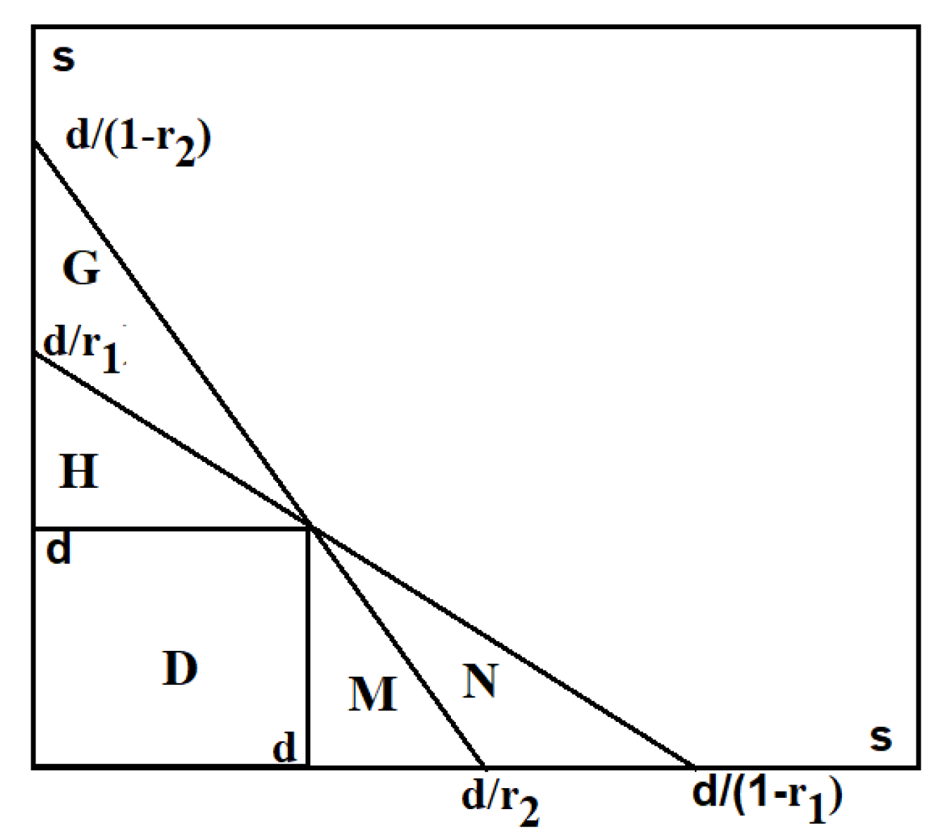
Since the probability for the non-diversified system is given by the (normalized) area of the square
D in
Figure 1 and the probability of joint default is given by that of the area of the combined regions
the validity of (
1) is clear.
Even though the case depicted in
Figure 1 is one of several possible cases considered in
Wagner (
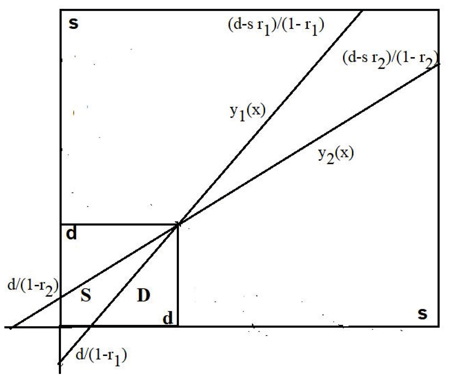
2010), he considered diversified portfolios without short positions. One of the aims of this work is to extend Wagner’s theoretical analysis by including portfolios with short positions. We show that if we consider the generic case depicted in
Figure 2, that when each bank diversifies by including short positions on the other bank’s portfolio; then the probability of joint default decreases, even though the probability of each bank defaulting individually may increase. The other aim of this work is to point out a dilemma that confronts the risk managers and/or regulators: Should one minimize the probability of collective loss or minimize the joint risk of default? We show that each choice leads to a different strategic decision.
The remainder of this work is organized as follows. In
Section 2 we recall Wagner’s model. Since in that model the different probabilities of interest reduce to the computation of areas in a square of size
we describe the areas determined by the different portfolios geometrically. In
Section 3 and
Section 4 we consider the extensions of Wagner’s model. First, in
Section 3 we prove that when diversification includes short positions and leverage, the probabilities of default decrease with diversification. In particular, the probability of joint default or systemic crisis decreases. In
Section 4 we depart from Wagner’s model in that we consider portfolios with a return of arbitrary sign, and we shall see that in this model the probability of systemic crisis decreases when short positions are allowed. In
Section 5 we regard the problem from the point of view of risk theory. We carry out an analysis using the value at risk (VaR) (which is a non-coherent risk measure). Since we are considering Gaussian returns, the VaR happens to be the standard deviation, and this makes the analysis simple. Clearly, if one were to consider coherent risk measures, the risk of a diversified portfolio would always be less than the sum of the risks of the individual banks. In
Section 6 we collect some final remarks and discuss some implications of our results for risk managers and regulators. In
Appendix A we offer details of computations presented in previous sections. This paper can be seen as an extension of (
Cadenas et al. 2020); where short positions are not considered and there is no reference to Gaussian returns.
2. The Model
Using the same notations as in
Wagner (
2010), consider the financial positions of the two investors with diversified portfolios given by:
A bank run takes place whenever or which are the regions in the plane (respectively) bounded by the lines and Each bank is allowed to invest a share of their funds in the other’s bank portfolio. In the case of short positions, we say that each bank is allowed to short its portfolio anywhere in the range given by . After all, since the model assumes that each bank manages one unit of funds from risk-neutral investors, when considering short positions it is reasonable to assume that banks cannot short beyond one unit of funds.
Some Generic Observations about the Default Regions
In order to compute the probabilities of default, we begin by exploring the positioning of these lines as r varies. Denote by (resp. ) the equation of these lines. When we have the vertical line (infinite slope) through (resp. to we have the horizontal line ). The line rotates counterclockwise as increases from 0 to 1, and it rotates clockwise as decreases from 0 to . To see this, note that the slope of this line is thus the line is vertical for and increases from to 0 as increases from 0 to Similarly, rotates clockwise as increases from 0 to 1, and it rotates counterclockwise as decreases from 0 to . For the region (resp. for ) is the region to the left (resp, to the right) of the line (resp. ).
Finally, note that
and
rotate towards the diagonal as
Let us suppose that
and
are such that the lines are as in
Figure 2. The intercepts of the first line are
and
and those of the second line are
and
4. The Probabilities of Default in a Gaussian Model
Here we depart from Wagner’s model in the sense that
x and
y are considered to be the returns on the bank’s assets, and are supposed to be centered Gaussian random variables, with unit variance and correlation
That is, their joint distribution has a probability density
In this case, the range of is the whole plane. Once an admissible default threshold is agreed upon, the joint default region is the “orthant” If we consider the diversified portfolios and then the geometry of the default regions is as above, the lines that define the boundary of the default regions extend to infinity in both directions. At this point let us only note that the probability of loss of any of the banks is where stands for the cumulative distribution function of the standard normal random variable.
It is also clear that when
and
Wagner’s observations continue to be valid, that is, Equation (
1) holds true in this model as well. Let us now examine the effect of diversification depending on the type of diversification or leveraging.
4.1. The Probabilities of Loss of a Diversified Bank
The Gaussian model allows us to compute the probability of loss of the diversified portfolio. Note that
is a centered Gaussian random variable with variance
Therefore
Since or depending on whether or not, we have
Theorem 2. With the notations introduced above, it follows from (4) that: That is, shorting or leveraging decreases the probability of default for an individual bank.
The role that the standard deviation plays in this analysis, will reappear when we examine two standard risk measures, namely the VaR and the expected shortfall.
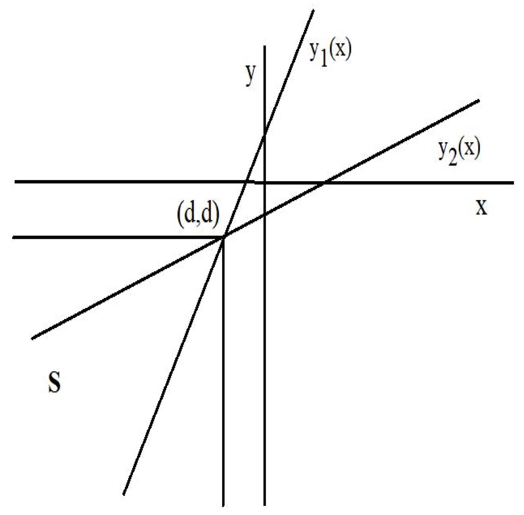
4.2. The Probability of Systemic Crisis
In the extended case, the region
S of default, that is
is the region between the lines
and
contained in the “orthant” determined by the half planes
and
as depicted in
Figure 3.
As the point
is on both lines as well as on the lines
and
as above, we might think of
as obtained by rotating
clockwise about
and
is obtained rotating
counterclockwise about
To be more precise
S in the 4th orthant contained between the lines defined by the angles:
when the origin of the coordinate system is put at
Note that when
then
and as
then
decreases to
That is
S tends to the region
We now clearly have:
Theorem 3. With the notations just introduced, when and the probability of joint default of the diversified portfolios satisfies: Proof. In principle
can be computed as
The problem is that the probability density of
is not invariant under translations nor under rotations, therefore, to go beyond this generic statement, we now suppose that
(that is, in this model we count any negative return as a loss). If we introduce polar coordinates
and
the probability
can be computed as
Integrating with respect to
r we obtain
□
We collect these remarks under the following statement.
Theorem 4. With the notations introduced above, the probability of systemic crisis is given by (6). We now draw some consequences form (
6).
Comments
(a) Note that is a increasing function of the coefficient of correlation
(
b) When
(the case considered by Wagner)
(
c) As
and
then since
and
in this particular case:
5. Risk Analysis
In this section, we shall verify that as then the risk of becomes larger than the risk of X when both are measured by the value at risk. Similarly, if we consider the total, or aggregated risk of the two diversified banks, the risk of the combined banks is larger than that of the combined non-diversified banks.
The value at risk (VaR) of a random asset of return
W, at confidence level
modeled by a continuous random variable, in units of the initial investment, is given by the solution (in
V) of
It is known that VaR is non-necessarily a coherent risk measure, despite the fact that it is enforced by regulators, and that it is very easy to estimate and interpret.
It is a standard exercise to verify that when
W is a centered Gaussian random variable:
5.1. The Risk of a Diversified Portfolio
The diversified portfolio
is a centered Gaussian with variance
Thus, according to (
7), the value at risk of
is
whenever
(and of course for
). That is, if me measure risk with VaR, entering a short or a leveraged position, increases the risk even though it decreases the probability of loss.
5.2. The Aggregated Risk
If we model the financial positions of the banking system by
in the same way that an individual bank would aggregate its risks, and we decide to measure the systemic risk by the value at risk, then, invoking (
7) once more we obtain:
This should be compared with the aggregated risk without diversification:
and the conclusion is clear. We sum up these computations as follows.
Theorem 5. If we we aggregate the risk in the system as then the value at risk at confidence level α satisfies Notice that as far as the total loss being more than we have Proof. The proof of the first part was established prior to the statement. It is a reflection of the fact that VaR may not decrease with diversification. As far as the proof of the second assertion, notice that on the one hand
and on the other
Note that whenever that is when both banks are equally diversified. In this case, the probability of loss in the aggregated portfolio does not depend on the diversification. □
6. Discussion
One of the controversies of diversification is that, although it may be beneficial for a bank in reducing the risk of its portfolio, it comes at the expense of increasing the likelihood of systemic risk. As banks diversify their portfolios, their business activities overlap and their portfolios become more similar to each other. This situation tends to expose the entire system to the same risks, and as a consequence, the probability of joint failure increases. In this line of reasoning, we extend the analysis by showing that when the returns of the bank’s assets are considered to be centered Gaussian random variables, as opposed to behaving under a uniform distribution as assumed by
Wagner (
2010), it continues to hold that diversification tends to increase systemic risk. However, a more important contribution of the paper is to show that when short positions are allowed; then the same measure of risk used by
Wagner (
2010) ends-up offering a different picture of diversification. That is to say, when short positions are allowed, diversification does not increase the probability of joint failure (i.e., systemic risk).
Furthermore, we show that not only the picture of diversification and systemic risk changes when short positions are allowed, but that the picture also changes when a different risk measure, like VaR, is used. We establish that when using VaR for evaluating short positions the risk of individual failure increases (rather than decreasing) with diversification; and also that the systemic risk decreases (rather than increasing) with diversification. These are the opposite conclusions than what we get when the risk measure is defined as in
Wagner (
2010). We would like to point out that one possible direct application of the idea of short positions could be the case of Government financial bailouts.
Our findings suggest a methodological problem, which consists of figuring out which of the two risk measures should be used and why. On one hand, we can pre-assign a tolerable loss threshold and then determine a portfolio that minimizes the probability of falling below the loss level. Or, on the other, we can fix a frequency of losses and then choose a portfolio that minimizes the loss with that frequency. Although these two procedures seem both to be equally reasonable; they can imply different views on diversification and, correspondingly, they assess individual and systemic risk in a different manner.
We don’t offer an ultimate solution to this problem here, but the finding in itself is relevant. Why? Because ambiguities of this sort generate a situation in which risk managers and regulators perceive risk in a manner that leads to opposite conclusions. Our findings are also relevant because we show that risk assessment changes depending on whether banks can assume a short position (capital leverage) or not. In addition, our results are suggestive of a host of problems that can be found in the literature about differences in risk perception in areas such as public health and tourism (
Wolff et al. 2019;
Renn 2004;
Cui et al. 2016;
Neuburger and Egger 2020), but for the case of banks. In the case of public health (
Renn 2004), the discussion usually revolves around communication, conflict resolutions, and delineating the different rationale behind risk measures; which in the case of the banking system will not be much different.
Finally, and perhaps most importantly, the results we have presented here are also suggestive of problems about differences in risk perception that are discussed in the behavioral finance literature (
Vlaev et al. 2009;
Ricciardi 2004,
Aren and Zengin 2016). Our work can be extended in various directions. One line of inquiry is to investigate whether allowing the system to consist of more than two banks would in any way change the conclusions. We are currently pursuing this line of work, following (
van Oordt 2014), for the case in which securitization is allowed. Another line of inquiry might be to study how results would change in the case of flat tails distributions. A third line of inquiry can be to work, with one of the risk measures as a reference, the implications to diversification and systemic risk when banks use a different risk measure. Observe that this would lead banks to have a different optimal solution, and the relation between them would be now of asymmetry (rather than symmetry). We do realize that attempting to find a solution to this problem purely in terms of a coordination problem between banks and regulators, may not result in an attractive line of attack because the way we assess the problem depends on what risk measure has been chosen by whoever happens to study the problem. However, we can choose a specific risk measure and investigate -from such a point of view- the implications for banks following different strategies in terms of the risk of individual and systemic failure.


