Small and Medium-Sized Enterprises, Business Demography and European Socio-Economic Model: Does the Paradigm Really Converge?

Abstract

Although the European business environment induces important premises and assures conditions in determining economic growth and social well-being, the determinant and existent connections between the evolution of small and medium-sized enterprises (SMEs), business demography characteristics and the European socio-economic model have been scarcely studied in recent years. The dimensions of the European socio-economic model design a very specific framework in developing business demography and assuring a favorable environment for future SME development. The main aim of the manuscript is to investigate the evolution of the European SMEs sector and the perspective of business demography evolution to converge with exigencies of the European socio-economic model. In order to argue the research objective, eight specific and representative business demography variables were employed, from 12 European Union member states (EU-MS), during 2009–2017. Further, the SMEs’ performances, determined by changing the economic functional paradigm, were assessed. For proving this, an econometric model was designed considering labor productivity as an endogenous variable. Our preliminary analysis shows considerable differences in business demography indicators and SMEs development among all five socio-economic sub-models of the main European socio-economic model, proving a tight connection between European socio-economic models and SMEs’ performance and arguing the necessity of a paradigm convergence. Within some sub-models, there is clear evidence of clustering and convergence in terms of business demography and SMEs future development.

1. Introduction

The European Economic Area and, implicitly, the European Union’s economy have undergone numerous and decisive reforms, highlighted in the existence of a mixture of economic models among the European Union member states. Our approach is dedicated to investigating the evolution of the European small and medium-sized enterprises (SMEs) sector and the perspective of business demography evolution to converge with exigencies of the European socio-economic model. From this perspective, the aim is to evaluate the response of the contemporary economies to numerous risks and challenges they are facing on their way to assuring growth and well-being for their populations. The big challenge of this research was to correlate the evolution of SME business demography during the analyzed period with the specificity characteristics of one of the European socio-economic model variants and integrate them in the econometric model.

In the European Union (EU), small and medium-sized enterprises (SMEs), during the period of long transformations has started to become a vital economic element in assuring both economic development and social wealth. As Gaganis et al. (2019) considered in their study, SMEs represent the backbone of economic activity in a large number of countries, including in the EU (Gaganis et al. 2019). De Marco et al. (2020) considered that SMEs are pertinent business instruments in shaping the innovation ecosystem, inducing important increases in economic growth and employment rates. According to Mura et al. (2020), the EU economic environment and circular economy (CE) practices are perceived as business opportunities for SMEs, being, at the same time, a favorable source of value creation. On the contrary, Johnstone (2020) held the view that SMEs define the biggest share in the EU contemporary economy and are responsible for most of the pollution. Masroor and Asim (2019) highlighted that a stable and very prosperous SME sector pushes the economic success of any country which understands its opportunity.

Further, a large body of literature continues to argue the importance, necessity, role and influence of the SME sector in providing vital functions in the architecture of contemporary economies. The World Trade Organization (WTO 2016) recognizes that SMEs play a crucial role in promoting international economic growth and their robustness contributes to diminishing the unemployment rate. The IEA (IEA 2015) highlights that almost 50% of the global gross value added is created by SMEs, as well as more than 13% of the global total final energy demand, while the share of SMEs in GDP varies between 16 and 80%. Moreover, in the literature, most of the existing studies analyzed the SME sector by providing evidence from individual countries, such as Ancarani et al. (2019), who conducted a comparative study regarding assessment of SME competitiveness for Italy, Canada and Hungary; Silva and Santos (2012), in the case of Portugal; Batrancea et al. (2018), for Romania; and Fitriati et al. (2020), for Indonesia, or by examining some of the specific characteristics such as capital structure and firm performance (Li et al. 2019), working capital (Afrifa and Padachi 2016), entrepreneurial orientation (Kiyabo and Isaga 2020), market orientation (Petzold et al. 2019), export (Tan et al. 2018), trade credit (McGuinness et al. 2018) or leverage (Chalmers et al. 2020). Cosenz and Bivona (2020) showed that SMEs are constantly subject to complex changes imposed by fast-changing markets which force them not only to be able to survive in conditions of aggressive competition but also to successfully orient themselves towards those business models and geographical spaces that will ensure their survival. Blanck et al. (2019) in their study remarked a positive correlation among business incubation and urban development which is often associated with the SME internationalization degree.

The evolution of the EU economy proves that the private economic initiative and private invested capitals are concentrated mainly in the SEMs sector which has already been recognized as a major economic component of the member states’ economies. With this consideration, the dimension of the small and medium-sized enterprises sector is highly important in EU economic architecture development. The European socio-economic model integrates SMEs as a fundamental pillar of the business model and the evolution of business demography could mainly be understood as reflecting a specific pattern of one of the existing variants of this economic model (hence resulting in economic SMEs’ performance).

The SMEs sector concentrates important economic, social and labor resources at the European level, being a fundamental component in both economic and business architectures. As is remarked in the literature (Özbuğday et al. 2020), SMEs provide a significant share of gross domestic product (GDP), generate employment for a numerous labor force, promote innovation and export and internalize local business opportunities. According to D’Imperio (2015), quoting the Edinburgh Group, the world SMEs sector represents 99% of all business sectors and employs almost 60% of the total workforce, while in the EU, the same sector employs approximately 90 million people with a yearly gross increase of 1.1 million (Muller et al. 2014).

Starting from the general consideration of existing numerous economic and social performance differences across European welfare models over time, in the literature, it was approached as one of the most important initiatives in Esping-Andersen’s classification of welfare models (Esping-Andersen 1990). Numerous literature studies and scholars have performed a vast investigation on the European social model patterns. Dima et al. (2018) pointed out that EU competitiveness and economic convergence are massively connected to innovation and education. Most approaches aimed to reveal the successful strategies for EU economic performance over time, how the different models cope with the new challenges of the socio-economic environment and what we can learn from the evolutions and approach of each model. Summarizing, in the literature (Aiginger and Guger 2005; Aiginger 2008; Guger et al. 2007; Burghelea et al. 2013), three variants of capitalist systems are mentioned: the Scandinavian system, which includes the Nordic countries (the social-democratic model), the Continental system (the conservative model) and the Anglo-Saxon system (the liberal welfare model). Within the EU, there are two other systems: the Mediterranean one, including southern countries (Aiginger 2008) (Guger et al. 2007), and the “Catching-up” system which includes the newest members, former communist countries, in which Romania is included (Aiginger and Guger 2005).

Further, the European SMEs are affected by numerous and undetermined business risks and uncertainties and they are working under intense economic pressures and asymmetric challenges; therefore, they need to approach alternatives to properly confront the economic adversities.

The main objective of this article is to look for certain factors that influence the economic performance of enterprises, to provide information for substantiating a general framework of EU socio-economic policies. The starting point was to investigate the hypothesis that the evolution of SMEs’ business demographics mainly reflects an available pattern of the European socio-economic model among EU countries. In doing so, in the manuscript, a dataset that includes SMEs’ most representative business demography indicators is analyzed, which allows a wider understanding of the influence of economic models on SME growth performance. Our research is focused on 12 EU countries over the period 2009–2017, which allows us to consider a significant number of business demography variables which vary in terms of SME economic depth of the activity and the country dimensions that we analyze.

Considering a dataset of eight representative business demography variables (nominal labor productivity per person and gross domestic product, population of active enterprises, births of enterprises, deaths of enterprises, persons employed in the population of active enterprises, persons employed in the population of births, persons employed in the population of deaths), operating in 12 EU countries over a period of eight years, we find that business demography developments and national economic dimensions have a statistically significant impact on converging to a specific economic performance.

Another feature of this work is that we focus on those business datasets that have a more homogenous variables sample distribution across the countries which could be assigned to one economic and social model or other economic and social models existing in the EU economy. As it is discussed in the literature, this consideration enables us to control the distribution of all those variables influencing the SME sector development due to business type differences and inland economic constraints.

From the methodological point of view, this research extends the contributions in the literature, in line with previous studies, by highlighting the need to perceive the complexity of business demography through the specific pattern perspectives of the European socio-economic model. Appropriate research methods and instruments used in carrying out the analysis were the panel data methodology and its subsequent techniques. Consequently, this method was used aiming to identify the existence of a specific pattern among the considered economies concerning the determinants of SME performance. In the related literature, there are many studies using this methodology in researching SME business demography, but the choice of using this methodology in this research was based on its robustness and the fact that it provides relevant information on the influences of determinants both transversally (from one country to another) and longitudinally (from one year to another).

This manuscript contributes to the existing literature in the field of European business models by considering SMEs’ different business variables and economic components of their activities, processes, developments and practices in converging the exigencies of the European socio-economic model framework.

Moreover, this practical review sheds light on the important role of SMEs in providing economic growth and stability in valuing the inland economic potential, as well as their economic behavior in the improvement of an appropriate variant of the economic model developed among the EU member states. Furthermore, this research encourages a proactive understanding of SME business demography by providing a constructive analysis environment between researchers, practitioners and policymakers. Practitioners and SME managers may improve and extend their knowledge in the field of European socio-economic model framework development by identifying the specific characteristics, risks, potentials and threats for implementing tools and adopting practices and lucrative strategies in valuing the strategic importance that business variables have for SMEs. For policymakers, this study highlights the key role of SMEs in the development of the EU economy and in providing economic and social wealth, supporting private initiatives and providing insights for better regulating the decision-making process and the business management requirements.

The paper content is organized as follows. The data and methods on the topic of the European socio-economic models and SMEs’ performance are presented in the second section as they are determinants in understanding the main business demography variables related to this research and the link between them and economic performance with approaches argued in the literature. Further, the research design including details about the methodology and scientific approach employed is presented in this section. The main findings of the research and the discussions incorporated by them are presented in the third section. The final section deals with the conclusions and limitations of the study.

2. Data and Methods

2.1. Data Sources

Following the research’s objectives, the study investigates the characteristics of SME business demography considering all five variants of the European socio-economic model, according to Aiginger and Guger (2005). The authors also consider that each model should be represented appropriately in the investigation. The analyzed data cover the period 2009–2017. The SME business demography specific data were retrieved from Eurostat (Eurostat 2020). Taking into account the differences in economic and social performance across European welfare models over time, starting with Esping-Andersen’s classification of welfare models (Esping-Andersen 1990), scholars have contributed to a vast body of literature on the European social model. Most approaches aimed to learn about successful strategies for Europe, how the different models cope with the new challenges of the socio-economic environment and what we can learn from the evolutions and approach of each model. Summarizing, three variants of capitalist systems are mentioned in the literature: the Scandinavian system, which includes the Nordic countries (the social-democratic model), the Continental system (the conservative model) and the Anglo-Saxon system (the liberal welfare model). Within the EU, there are two other systems: the Mediterranean one, including southern countries (Aiginger 2008) (Guger et al. 2007), and the “Catching-up” system which includes the newest members, former communist countries, in which Romania is included (Aiginger and Guger 2005).

Table 1. Synoptic of the five socio-economic models’ characteristics.

The Socio-Economic Models	Countries	The Main Characteristics
The Scandinavian Model	Denmark, Finland, Sweden, Iceland	- High degree of redistribution - The most efficient system of social protection - Promoting social inclusion
The Continental Model	Austria, Belgium, French, Germany, Luxembourg, Netherlands	- The labor market is governed by state - Employment is the basis of social transfers - The granted benefits are low, being dependent on the previous income level - The taxation level is high - A lower inequality of the incomes than of the countries in the Anglo-Saxon model as a result of higher spending on social protection in the past
The Anglo-Saxon Model	Ireland, United Kingdom	- Liberal approach to the welfare system - Social assistance is limited - State responsibility is transferred to the care of individual both in terms of insurance system and in terms of labor market regulation - Employment is relatively high - In terms of equity, there are notable differences in the distribution of income in society
The Mediterranean Model	Greece, Italy, Portugal, Spain, Cyprus, Malta	- The state has a minimal role in terms of social protection - Family plays an important role both socially and in productive plan - The labor market is controlled by the state, and it is highly fragmented and rigid - In the long term, the unemployment rate is very high, especially among young people, although the social expenditure budget is low
The “Catching-up” Model	The Visegrad countries: Czech Republic, Hungary, Slovakia, Poland (Bulgaria, Estonia, Latvia, Lithuania, Romania, Slovenia) *	- Regulated labor market - Still underdeveloped institutions of social dialogue - A low level of security

* This is a comprehensive approach, which has taken into account both the typologies of social models in the European Union and the analysis of competitiveness. Source: the authors, based on Sima et al. (2015) and Burghelea et al. (2013).

summarizes the main features of the five social-economic models above-mentioned.

In the research, the latest available datasets on the Eurostat website for seven variables were used. As no complete datasets were found for all European Union countries, only the results from 12 countries were used in performing the analysis (

Table 2. Countries that have been data sources.

Country	Model
Belgium	The Continental Model
Bulgaria	The “Catching-up” Model *
Czech Republic	The “Catching-up” Model
Denmark	The Scandinavian Model
France	The Continental Model
Germany	The Continental Model
Hungary	The “Catching-up” Model
Italy	The Mediterranean Model
Romania	The “Catching-up” Model *
Spain	The Mediterranean Model
Sweden	The Scandinavian Model
United Kingdom	The Anglo-Saxon Model

* These two countries has become EU-Member States after the Catching-up” Model has been defined Source: performed by the authors.

).

This study analyzed data extracted from the business demography data collection regarding the structure and performance of businesses in the specified countries, aiming to assess the main risks which can affect SME performance. In the table below, the data series considered in designing the research and the symbols used for designating each series are presented (

Table 3. Variable descriptions and data series availability.

Symbol	Variable Description
lab_prod	Nominal labor productivity per person-percentage of EU27 (from 2020) total (based on million PPS), current prices
gdp_per_cap	GDP per capita in PPS
act_ent	Population of active enterprises in t-number
birth_ent	Births of enterprises in t-number
death_ent	Deaths of enterprises in t-number
pers_emp_act_ent	Persons employed in the population of active enterprises in t-number
pers_emp_births	Persons employed in the population of births in t-number
pers_emp_deaths	Persons employed in the population of deaths in t-number

Source: the authors, based on Eurostat (2020).

).

The datasets are annual, spreading over nine years, from 2009 to 2017. The beginning is 2009, as we considered this time as a turning point in the evolution of the EU, 2007 being the year in which the last enlargement of the EU took place, and, subsequently, we considered that after two years, the effects became visible.

Table 4. The descriptive statistics of the datasets.

	Lab_prod	Gdp_per_ cap	Act_ent	Birth_ent	Death_ent	Pers_emp_ Act_ent	Pers_emp_ Births	Pers_emp_ Deaths
Mean	4.519	97.370	13.898	11.521	11.388	15.593	11.925	11.766
Median	4.654	106.000	13.651	11.325	11.326	15.212	11.785	11.664
Maximum	4.881	131.000	15.201	12.839	12.670	17.183	13.650	13.562
Minimum	3.681	44.000	12.256	9.932	9.724	14.102	9.853	9.610
Std. Dev.	0.323	27.165	0.946	0.917	0.951	0.963	1.002	1.112
Skewness	−1.156	−0.589	−0.079	0.014	−0.144	0.223	−0.131	−0.180
Kurtosis	3.190	2.059	1.656	1.488	1.566	1.471	1.871	1.868
Jarque–Bera	24.228	10.218	8.240	10.289	9.632	11.410	6.048	6.357
Probability	0.000	0.006	0.016	0.006	0.008	0.003	0.049	0.042
Sum	488.057	10,516.000	1501.025	1244.293	1229.903	1684.026	1287.853	1270.739
Sum Sq. Dev.	11.180	78,957.190	95.714	89.914	96.744	99.261	107.516	132.409
Observations	108	108	108	108	108	108	108	108

Source: the authors’ own computations.

contains the descriptive statistics of the datasets considered in the paper. Due to the fact that the common range of data availability is 2009–2017 and the present reserch is based on the panel data approach, the considered period is set accordingly.

The results of the correlation analysis are presented in

Table 5. Results of the correlation analysis.

Correlation	Lab_prod	Gdp_per_ cap	Act_ent	Birth_ent	Death_ent	Pers_emp_ act_ent	Pers_emp_ Births	Pers_emp_ Deaths
Probability
lab_prod	1.0000 -----
gdp_per_ cap	0.9302	1.00000
	0.0000 *	-----
act_ent	0.4178	0.2496	1.0000
	0.0000 *	0.0092 *	-----
birth_ent	0.2845	0.1296	0.9640	1.0000
	0.0028 *	0.1812 *	0.0000 *	-----
death_ent	0.1829	0.0536	0.9154	0.9448	1.0000
	0.0582 *	0.5814 *	0.0000 *	0.0000 *	-----
pers_emp_ act_ent	0.3710	0.2762	0.9483	0.9499	0.9228	1.0000
	0.0001 *	0.0038 *	0.0000 *	0.0000 *	0.0000 *	-----
pers_emp_ births	0.1548	0.0093	0.9123	0.9681	0.9324	0.9401	1.0000
	0.1096 *	0.9241 *	0.0000 *	0.0000 *	0.0000 *	0.0000 *	-----
pers_emp_ deaths	0.0829	−0.0568	0.8640	0.9272	0.9614	0.8887	0.9571	1.0000
	0.3939 *	0.5593 *	0.0000 *	0.0000 *	0.0000 *	0.0000 *	0.0000 *	-----

* Probability indicating the significance of t-statistic at 5%. Source: the authors’ own computations.

. According to this analysis, the results are not significant for three variables: death_ent, pers_emp_births and pers_emp_deaths reported as gdp_per_cap, which does not contradict the economic theory. In emerging economies, such as Catching-up countries, the firms’ life cycle is still short, being below the EU average (Shirokova et al. 2014). However, this led us to study these indicators.

Assuming labor productivity is one of the most important indicators of economic growth of SME activity, we designed a model considering this as an endogenous variable. The main research objective emphasizes the relationship among nominal labor productivity and the business demography variables described in Table 3.

2.2. Theoretical Methodology Description

The availability of data was limited, which led to significant restrictions in the choice of methodology. This is the main limitation of the research. This is also the reason that the paper aims to only identify new possibilities to develop the most efficient economic policy tools. In designing the current research, the main instrument used in carrying out the analysis was the panel data methodology and its subsequent techniques. This method was used aiming to identify the existence of a specific pattern among the considered economies concerning the determinants of SME performance. The choice of using this methodology was based on its robustness and the fact that it provides relevant information on the influences of determinants both transversally (from one country to another) and longitudinally (from one year to another).

The panel data regression model has a double index on its variables, the general form of the model being

$$Y_{it}={\beta }_0+{\displaystyle \sum }_{it,k}{\beta }_k{X}_{it,k}+{\nu }_{it}$$

(1)

where:

• i is the unit of observation, showing the cross-sectional dimension;
• t is the period of time, showing the temporal dimension;
• k indicates the kth explanatory variable;
• ${\beta }_0$ is the intercept;
• ${\beta }_k$is the coefficient of each explanatory variable;
• ${\nu }_{it}$ is the error term, which can be decomposed into two components: a cross-sectional unit-specific error, and an idiosyncratic error:

  $${\nu }_{it}=a_i+u_{it}$$

  (2)

Accordingly, (1) becomes

$$Y_{it}={\beta }_0+{\displaystyle \sum }_{it,k}{\beta }_k{X}_{it,k}+a_i+u_{it}$$

(3)

Thus, if eliminating some part of them, we would obtain a better result in terms of minimizing concerns for an omitted variable bias caused by unmeasured unit-specific factors. The first one does not change over time and the second one varies over the cross-sectional units and time. The constant error of time and the error specific to the unit, $a_i$, are unnoticed factors, which can be considered invariant in time, being very difficult to measure. Thus, the ordinary least squares (OLS) model does not differentiate $a_i$ from other types of errors, while the fixed effects (FE) model considers it as coefficients to be evaluated and the random effects model treats it as random variables (Baltagi 2013), (Greene 2002) (Gujarati 2003) (Maddala and Lahiri 2009) (Wooldridge 2006). The Hausman test is the procedure used to decide which technique or estimator should be adopted between the fixed effects within-group estimator (fixed effects model) and the random effects estimator. Assuming a non-stationary and cointegrated panel with endogenous variables, Granger non-causality tests are an essential tool in the application of cointegration techniques. These allow, on the one hand, the establishment of the error correction mechanism (ECM) and, on the other hand, the exploration of the relationships between the examined variables. Before that, the stationarity and cointegration of the data series must be verified. For that, the augmented Dikey–Fuller (ADF) test was used which consists in estimating the following regression model:

$$\Delta Y_t={\beta }_1+{\beta }_{2t}+\delta Y_{t-1}+{{\displaystyle \sum }}_{i=1}^p{\alpha }_i\Delta Y_{t-i}+{\epsilon }_t$$

(4)

where:

• $Y_t$ is the variable tested for stationarity;
• $\delta$ represents the lags used to identify possible higher-order autocorrelations;
• ${\epsilon }_t$ is the white noise error term.

According to Bond (2002), the null hypothesis in the case of the ADF test is $H_0: \delta =0$, against the alternative hypothesis $H_A: \delta <1$.

The test procedure is the same as for the Dikey–Fuller (DF) test: once the value of the DF test is calculated (5), it can be compared with the relevant critical value for the DF test. Therefore, the more negative the value of the ADF statistical test, the stronger the rejection of the null hypothesis.

$$DF\tau =\frac{\widehat{\tau }}{SE(\widehat{\lambda )}}$$

(5)

Testing the hypothesis for whether there is a statistically significant long-term connection between time series can be conducted by applying the Johansen cointegration procedure. To model cointegration, the basic steps of the Johansen methodology are as follows (Johansen 1991):

• Specifying and estimating a $\mathrm{VAR}\left(\mathrm{p}\right)$model (vector autoregression) for $Y$:

  $$Y_t=A_1{Y}_{t-1}+\dots +A_p{Y}_{t-p}+{\epsilon }_t$$

  (6)

  where:
  • $Y_t$is the vector of the variables $I\left(1\right)$;
  • ${\epsilon }_t$is the vector of innovations (or shocks).
• Rewriting the $\mathrm{VAR}\left(\mathrm{p}\right)$model to determine the number of integrated vectors:

  $$\Delta Y_t=\mathsf{\Pi }{Y}_{t-1}+{{\displaystyle \sum }}_{i=1}^{p-1}{\mathsf{\Gamma }}_i{Y}_{t-1}+{\epsilon }_t$$

  (7)

  where

  $$\mathsf{\Pi }={\displaystyle \sum }_{i=1}^p{A}_i-I$$

  $$\mathsf{\Gamma }=-{\displaystyle \sum }_{j=i+1}^p{A}_i$$
• Imposing normalization and identifying constraints on cointegration vectors resulting from considering a rank $r<k$for the coefficients matrix $\mathsf{\Pi }$.
• Estimation of the resulting vector error correction (VEC) cointegration model.

In Granger’s approach (Granger 1969), X is a cause of Y if it is useful in predicting Y, considering only past values of Y. The Granger causality test was applied in a VAR sense for testing the simultaneity of all variables considered.

According to Engle and Granger (Engle and Granger 1987), integration analysis is the appropriate technique to highlight the existence of a long-term stationary relationship between integrated variables. Two or more non-stationary data series can exist as a stationary linear combination if they are cointegrated. According to Hoffman and Rasche (Hoffman and Rasche 1996), the loss of information in a long-term relationship between the variables induced by differentiation can be avoided by using a vector error correction model (VECM). The VECM is appropriate to estimate a long-run relationship, providing efficient coefficient estimates. The VECM estimating procedure consists of four stages. First, it is necessary to test the panel unit for the unit root. The second stage is the identification and estimation of a vector autoregressive model of the integrated series. The third step is the VAR model selection and appropriate lag order, according to Equation (6). The procedure ends with the indication of the rank of the cointegration equation and the estimation of the model, according to Equation (7). Panel data modeling allows the analysis of the dynamic adjustment process, which cannot be conducted in a simple dataset with cross-sections. In this particular case, the generalized method of moments (GMM) was not an option because of the dataset’s characteristics. According to Arellano and Bond (1991) and Arellano and Bover (1995), it provides a more efficient estimator when T is small and N is large, which is not happening in this case.

3. Results

3.1. The Analysis of the Variables in Different Socio-Economic Models during 2009–2017

The issues of how the different models cope with the new challenges of the socio-economic environment were addressed by researchers who aimed to identify growth drivers and key areas for adaptability to present and future challenges (Aiginger 2008) (Aiginger and Guger 2005) (Esping-Andersen 1990) (Guger et al. 2007). From our perspective, in the context of the increasing risks that economies are facing, it is important to find what we can learn from each model’s evolutions and approach. Given that the differences in economic performance between European countries increased in the 1990s, especially in terms of production dynamics, productivity and employment, most of these scientific contributions examine differences in performance between European countries, seeking to identify the factors growth and key areas for adaptability to present and future challenges.

Our study started with an analysis of the evolution of the variables in categories of countries. Countries involved in the analysis were selected considering the European model and under the current socio-economic models, as shown above.

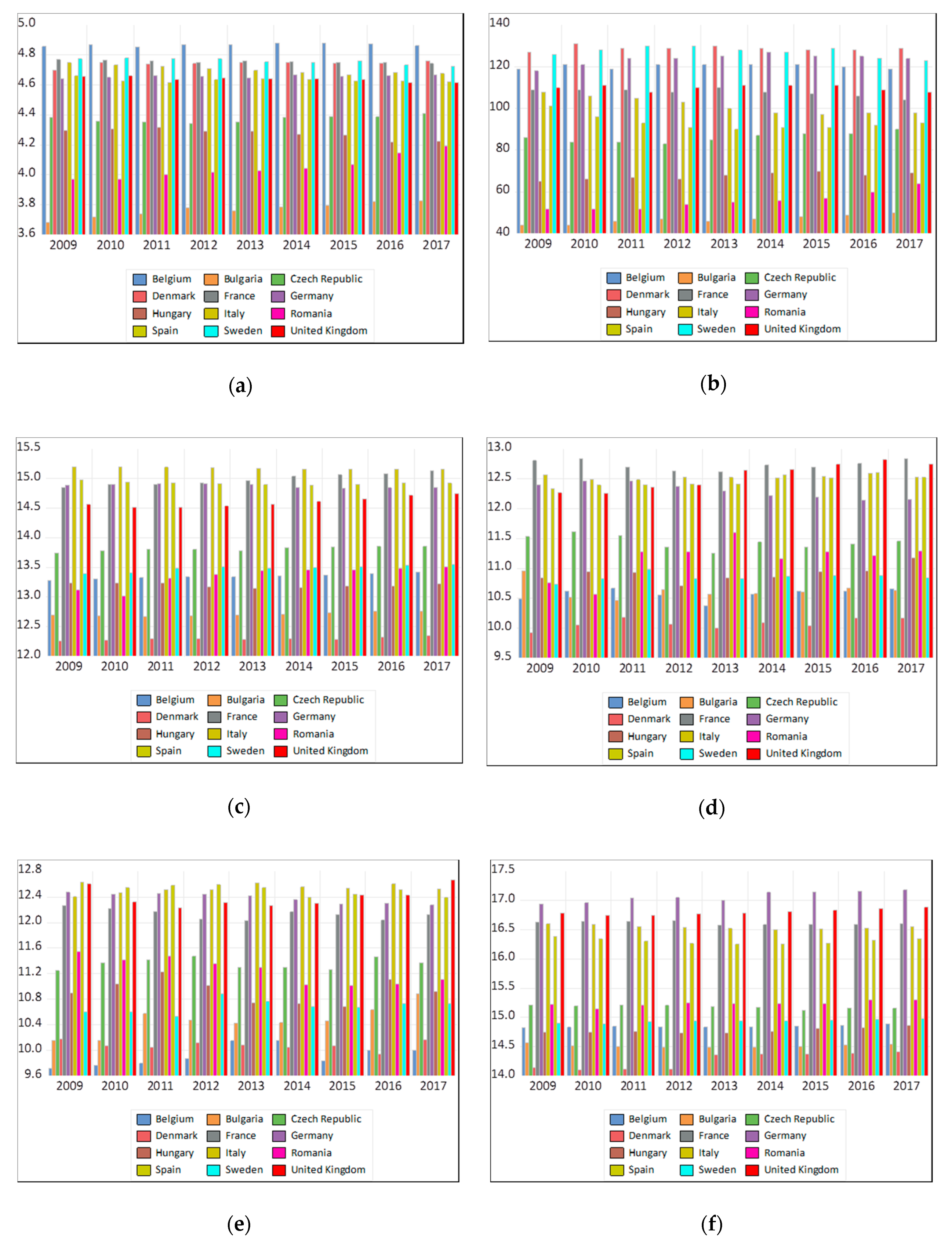
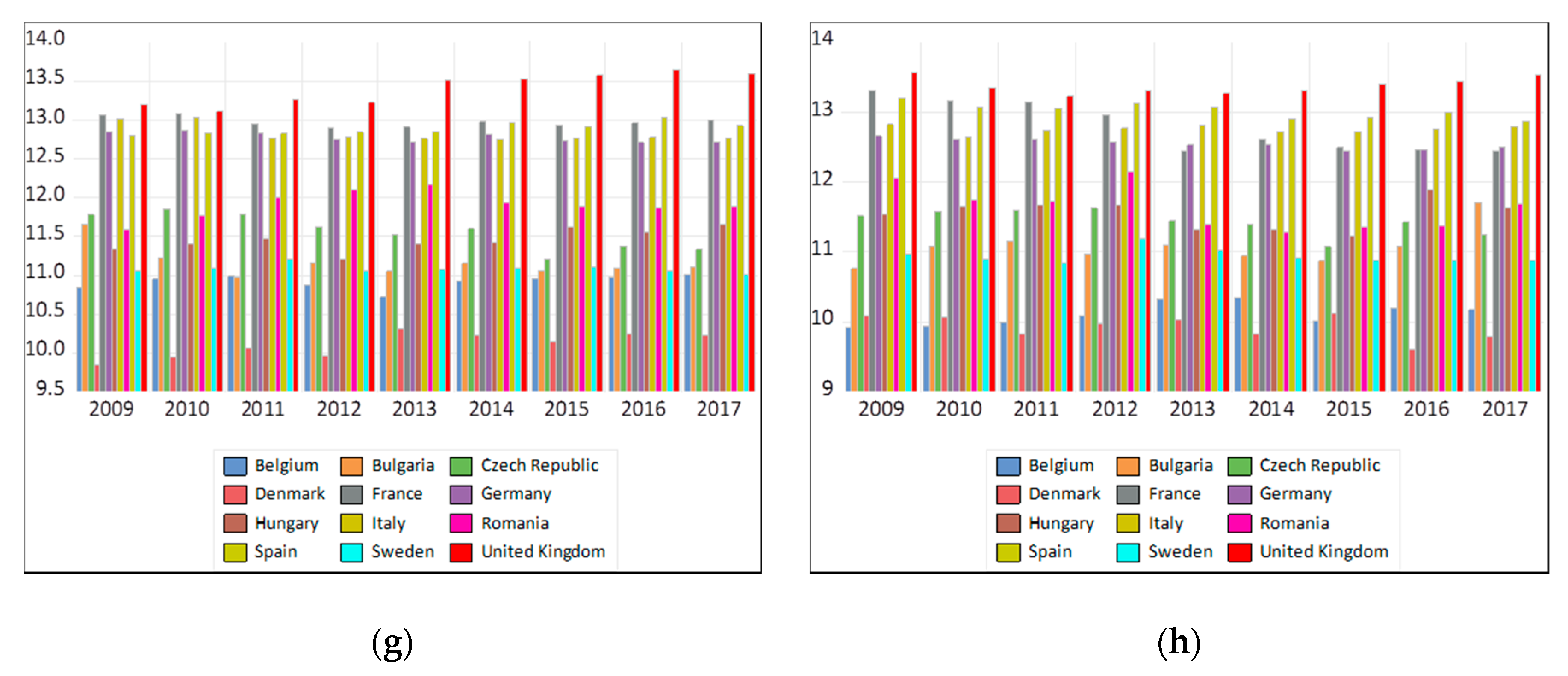
As we show above, we chose nominal labor productivity per person employed as a dependent variable, expressed, according to ESA (2010), as GDP per person employed, being intended to give an overall impression of the productivity of national economies expressed in relation to the European Union average (Eurostat 2007). By analyzing the evolutions of the variables at the country level, from Figure 1, their belonging to the stated socio-economic models is confirmed.

These differentiated evolutions are determined by the different rhythms of changes, imposed by the economic and technological environment, and the cultural one. It shows the importance of adapting European welfare states. As noted by Fagerberg et al. (2016), the global capitalist economy is not a unitary, homogeneous economy. Still, on the contrary, it is made up of countries with very different levels of economic and technological development. Starting from this finding, in the EU, it can be noticed that states have varying levels of development or technical structure, despite the accentuated process of economic convergence. Analyzing the ease of doing business (Rogge and Archer 2021) finds important differences among new and older EU member states in terms of performance and degree of convergence.

Referring to the evolution of the European economic model, Palevičienè et al. (2014) considered that EU member states, but especially those in the last wave of accession, under the influence of the need for convergence, change their social model. They are trying to apply those measures and policies that have proven effective in ensuring economic growth and the well-being of citizens. This statement is supported by the evolutions that Figure 1 exhibits.

The adaptation to the demands of the global economy has required a broad process of transformation of classical European paradigms and valorization of the new opportunities and development potentials. This has led both to the consolidation and improvement of the European economic model, but also the expansion of the economic models already existing in the EU area. On the other hand, as some studies highlighted (Fagerberg et al. 2010), the Catching-up economies are contextually different both from the developed countries and among them.

Reducing existing economic disparities, ensuring and promoting an environment conducive to economic development and capitalizing on existing potentials still hide levels and differences in the convergence between EU member states. Therefore, achieving sustainable economic growth, but mostly favorable to inclusion and resilience, requires, in the conditions of diversification of global economic demands and transformations, the application of a balanced economic policy, dedicated to ensuring a high degree of competitiveness in the context of consolidating market stability and reducing macroeconomic imbalances. Referring to these aspects, some scholars (Holzinger and Schimmelfennig 2012) (Loth and Paun 2014) argued that the differentiated integration of states in the European economic model just comes from the high degree of heterogeneity across EU member states, as a result of different rounds of negotiation and extension, but also from the design and functioning of the decision-making system at the EU level.

As studies have shown (Porter and Rivkin 2012), achieving a national economy’s fundamental objectives is supported by companies operating within it to face global competition. For this reason, it is essential to identify the critical convergence factors—social, institutional, economic and technological—of the environment that will support companies in the global competitive environment.

3.2. Empirical Analysis

As presented in the previous paragraph, despite the common policy at the European Union level in terms of the level of development, there are still significant disparities between member countries. These determined the choice of countries according to the socio-economic model, a factor that led to homogeneous characteristics within the respective groups. Data modeling using the panel method allows for heterogeneity control.

Our panel consists of 12 countries which were all member states of the European Union in 2018. The availability of data was limited, which restricted the analyzed period in 2009–2017. The use of Eurostat data ensures the compatibility of the variables between the countries considered, with the reporting methodology requiring their compatibility across the member states.

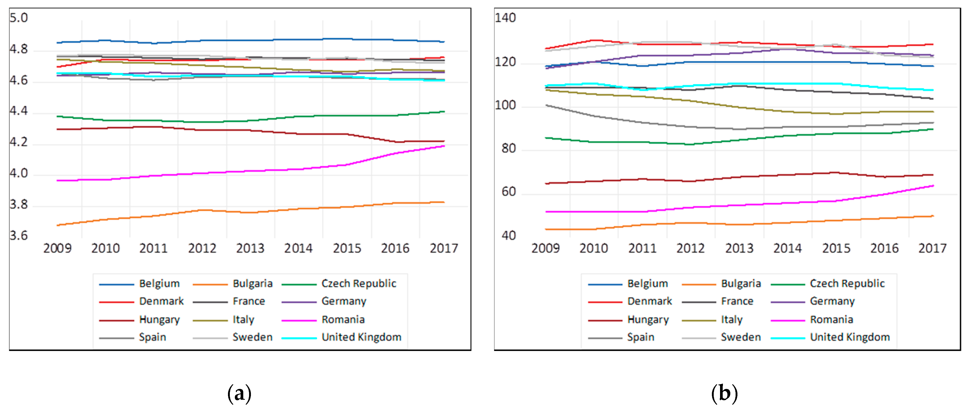
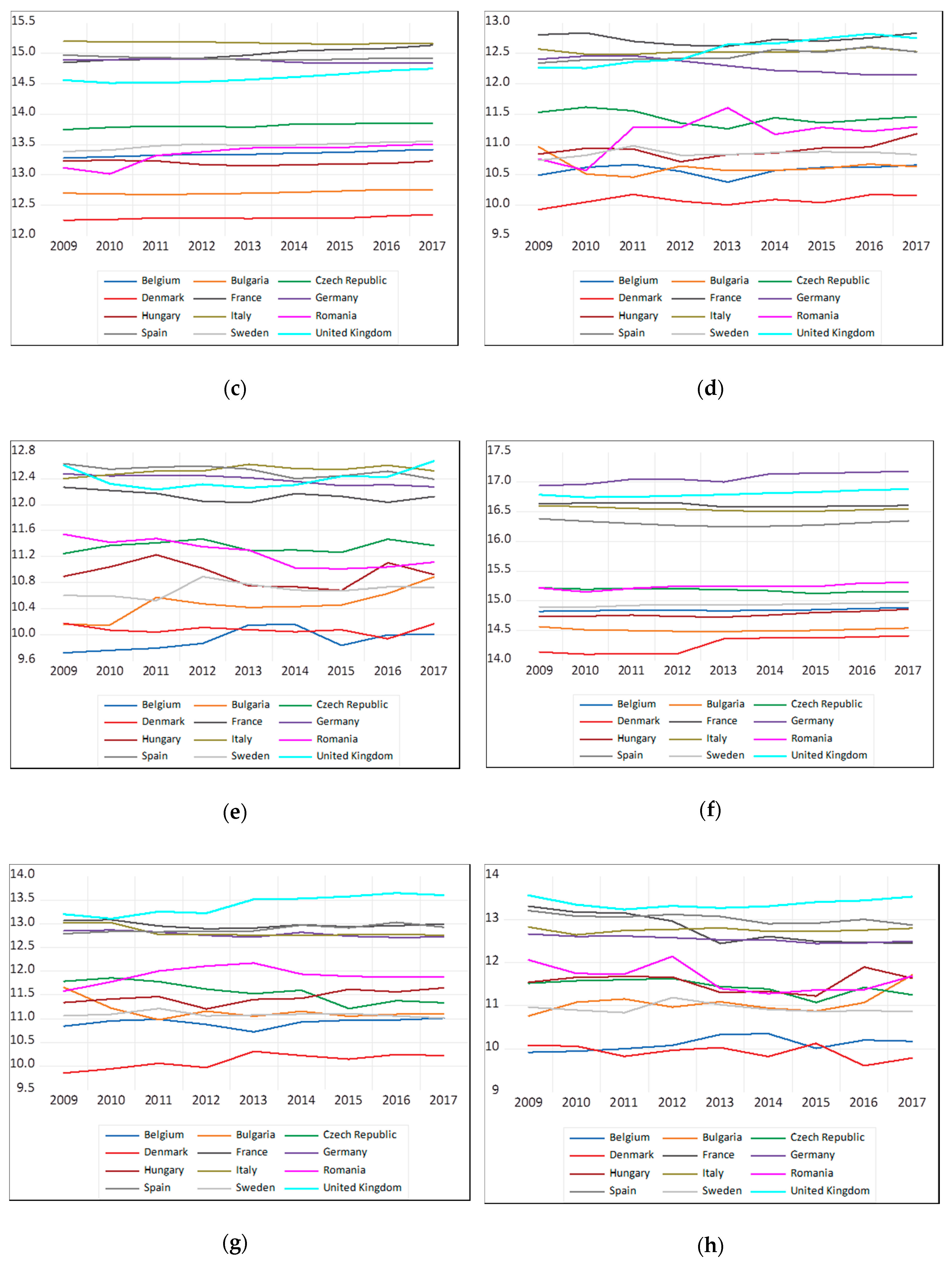
The empirical analysis uses time series for the data considered. The graph for each series shows the clear trends (Figure 2). This behavior suggests the need to test the stationarity of the series. Stationarity of a series implies that its mean, variance and covariance are constant over time. Otherwise, the series considered to be non-stationary has a unitary root, exhibiting a randomized series.

3.3. Stationarity and Cointegration

To identify the existence of a one-way relationship, from one direction to another, or the presence of a two-way connection, between two or more macroeconomic variables, the most indicated methods are Granger-type causality, the Johansen cointegration procedure, the autoregressive vector model (VAR), the vector error correction (VEC) model or the panel data models. Therefore, we aimed to investigate two main aspects: the first is to determine whether the variables are cointegrated, and the second is to identify the direction of causality between the variables.

The result of Jarque–Bera test statistics is that all series data do not have a normal distribution. Therefore, for all variables except gdp_per_cap, the natural log of the variables was used. In addition, this transformation reduces their variance.

The Hausman test was used to compare the random effects estimator to the “within” estimator. The null hypothesis of the test that the composite error term (random effects) is not correlated with the explanatory variables in the model, meaning that the fixed effects estimator is not applicable, was accepted.

The figures resulting from running the Hausman test are presented in

Table 6. Hausman test.

Test Summary	Chi-Sq. Statistic	Chi-Sq. d.f.	Prob.
Cross-section random	8.084177	7	0.3252

The authors’ compilation.

. The random effects model treats random effects as independent of explanatory variables, meaning that the investigators make unconditional inferences about the population of all effects. The main advantage of the random effects estimator is that it uses fewer degrees of freedom in estimation, allowing the inclusion of invariant covariates over time. The main disadvantage of the model is the assumption that the random effects are independent of the explanatory variables included. It is quite plausible that there may be unobservable attributes not included in the regression model that are correlated with the observable characteristics. This model, unlike the fixed effects model, does not allow the elimination of omitted heterogeneous effects.

Beyond the analysis of evolution graphs over time, the study of the regression model can provide some clues about the unit root.

Table 7. The estimators of the regression model.

Variable	Coefficient	Std. Error	t-Statistic	Prob.
lab_prod	3.316218	0.185441	17.88291	0.0000
gdp_per_cap	0.011900	0.000499	23.85434	0.0000
act_ent	0.295474	0.036962	7.994036	0.0000
birth_ent	−0.082856	0.056597	−1.463963	0.1463
death_ent	−0.046097	0.043987	−1.047970	0.2972
pers_emp_act_ent	−0.300072	0.045672	−6.570198	0.0000
pers_emp_births	0.149194	0.060087	2.482958	0.0147
pers_emp_deaths	0.026937	0.038739	0.695342	0.4885

The authors’ own computations.

shows the results of the regression model.

From the figures resulting from running the Hausman (Table 6), it is obvious that the fixed effects model is not applicable. The estimators of the regression model and the summary output of the model are presented in Table 7 and

Table 8. The summary output of the regression model.

Regression Statistics		Regression Statistics
Root MSE	0.073814	R-squared	0.947364
Mean dependent var	4.519044	Adjusted R-squared	0.943679
S.D. dependent var	0.323236	S.E. of regression	0.076710
Akaike info criterion	−2.226376	Sum squared resid.	0.588446
Schwarz criterion	−2.027699	Log likelihood	128.2243
Hannan–Quinn criter.	−2.145820	F-statistic	257.1199
Durbin–Watson stat	0.073967	Prob(F-statistic)	0.000000

The authors’ own computations.

. According to these results, GDP per capita, population of active enterprises, births of enterprises, deaths of enterprises, persons employed in the population of active enterprises, persons employed in the population of births and persons employed in the population of deaths represent causal variables for nominal labor productivity per person. The figures in

Table 9. Panel unit root tests summary.

Variable	Method	Levin, Lin and Chu t *		Im, Pesaran and Shin W-Stat		ADF-Fisher Chi-Square		PP-Fisher Chi-Square
		Statistic	Prob. **	Statistic	Prob. **	Statistic	Prob. **	Statistic	Prob. **
lab_prod	Level	−2.113	0.017	0.282	0.611	31.891	0.130	38.786	0.029
	1st difference	−11.147	0.000	−4.638	0.000	71.483	0.000	102.780	0.000
gdp_per_cap	Level	−0.172	0.432	0.957	0.831	27.754	0.271	37.257	0.041
	1st difference	−7.059	0.000	−2.41915	0.0078	48.1942	0.0024	80.967	0.000
act_ent	Level	−9.398	0.000	−1.03242	0.1509	32.6273	0.1122	15.5051	0.9051
	1st difference	−8.260	0.000	−2.98963	0.0014	52.7067	0.0006	53.574	0.001
birth_ent	Level	−4.240	0.000	−2.08438	0.0186	42.228	0.0122	47.213	0.003
	1st difference	−14.109	0.000	−5.75158	0	79.4625	0	98.385	0.000
death_ent	Level	−3.187	0.001	−1.04951	0.147	32.5552	0.1138	41.659	0.014
	1st difference	−9.000	0.000	−3.46019	0.0003	58.2316	0.0001	68.963	0.000
pers_emp_act_ent	Level	−0.534	0.297	2.13455	0.9836	13.290	0.961	11.919	0.981
	1st difference	−3.862	0.000	−2.66276	0.0039	50.5099	0.0012	80.585	0.000
pers_emp_births	Level	−9.866	0.000	−3.64779	0.0001	50.8991	0.0011	48.421	0.002
	1st difference	−10.628	0.000	−5.01694	0	75.9212	0	102.927	0.000
pers_emp_deaths	Level	−4.039	0.000	−1.2138	0.1124	31.964	0.1279	35.1677	0.066
	1st difference	−13.379	0.000	−5.62075	0	76.6516	0	85.9688	0

* 5% confidence level; ** Probabilities for Fisher tests were computed using an asymptotic chi-square distribution. All other tests assume asymptotic normality. The authors’ own computations.

show that the cointegration condition of the panel has been met.

Looking at the R-squared value in Table 8, as it is above 0.9, it may suggest that the variables are non-stationary. More than that, as the R-squared value obtained from the regression is higher than the Durbin–Watson (DW) statistic, at a low DW statistic, this evidence suggests a positive first-order autocorrelation of the error terms (Table 8), being a clear indication that this regression is spurious. This is also a clue for the non-stationarity of the series. These were arguments for the unit root panel tests.

Although the root of the panel unit is not a fundamental problem in approaching the panel data, especially in cases with a relatively short time series, as in the present paper, unit root tests have been used to test the information efficiency. The outcome of unit root testing matters for the empirical model to be estimated.

Table 9 summarizes the results of the panel series stationarity tests. The figures show that the data are not stationary at level, except for birth_ent and pers_empl_births, but they all become stationary at the first difference. In this condition, the condition of panel cointegration has been fulfilled.

According to the figures in

Table 10. Kao residual cointegration test results.

Test Summary	t-Statistic	Prob.
	−4.664259	0.0000
Residual variance	0.000797
HAC variance	0.000916

The authors’ own computations.

, there is cointegration among the series. This assumption implies that the series in question are related and therefore can be combined in a linear model.

3.4. The VAR Model Specification

As the variables are cointegrated, both the short-run (VAR) and long-run (VEC) models can be constructed. In the VAR models, there are no exogenous variables; all the variables are endogenous. The dependent variable is a function of its lagged values and the lagged values of the other variables in the model. The VAR model is estimated by ordinary least squares (OLS). The test results of the information criterion, namely, Akaike information criterion (AIC), Schwarz criterion (SC), and Hannan and Quinn criterion (HQC), impose the optimal number of lags.

Table 11. VAR lag order selection criteria.

Lag	AIC	SC	HQ
0	8.021805	8.253311	8.114869
1	−16.45875 *	−14.37519 *	−15.62117 *
2	−16.45815	−12.52255	−14.87607

* indicates lag order selected by the criterion. The authors’ own computations.

shows that all the variables have an optimal lag structure of one. From the Durbin–Watson statistics values which are closed to two, we can conclude that this model does not suffer from serial correlation. Analyzing the model coefficients, because most of them were not statistically significant, a Wald test was conducted for the coefficients’ diagnosis, as Zapata and Rambaldi (1997). After removing the redundant variables from the model, according the results of the Wald test, a new parsimonious model was obtained:

$$\begin{gathered} lab\_pro{d}_t=-0.0004gdp\_per\_ca{p}_{t-1}+0.9927lab\_pro{d}_{t-1}-0.0090pers\_emp\_death{s}_{t-1} \\ +0.0292pers\_emp\_act\_en{t}_{t-1} \end{gathered}$$

(8)

$$gdp\_per\_ca{p}_t=0.9523gdp\_per\_ca{p}_{t-1}+2.9753pers\_emp\_act\_en{t}_{t-1}-2.1381pers\_emp\_birth{s}_{t-1}$$

(9)

$$act\_en{t}_t=- 0.0295pers\_emp\_death{s}_{t-1}+0.0812pers\_emp\_birth{s}_{t-1}+ 0.9760act\_en{t}_{t-1}$$

(10)

$$birt\_en{t}_t=0.6573birth\_en{t}_{t-1}+0.2938lab\_pro{d}_{t-1}+ 0.1179pers\_emp\_death{s}_{t-1}$$

(11)

$$death\_en{t}_t=0.8703death\_en{t}_{t-1}+0.1034pers\_emp\_birth{s}_{t-1}$$

(12)

$$pers\_emp\_act\_en{t}_t=1.0136pers\_emp\_en{t}_{t-1}$$

(13)

$$pers\_emp\_death{s}_t=0.6252pers\_emp\_death{s}_{t-1}+0.3952pers\_emp\_birth{s}_{t-1}$$

(14)

$$\begin{array}{ll}pers\_emp\_birth{s}_t& \\ & =-0.1166birth\_en{t}_{t-1}- 0.0053gdp\_per\_ca{p}_{t-1}+ 0.4426lab\_pro{d}_{t-1}\\ & +0.1728pers\_emp\_death{s}_{t-1}+0.2441pers\_emp\_act\_en{t}_{t-1}+0.7646pers\_emp\_birth{s}_{t-1}\\ & -1.7020\end{array}$$

(15)

In this new VAR model, all the coefficients are statistically significant at p = 0.01, except for c(57) = −0.0053 and c(68) = −0.0295, which are significant at p = 0.05. According to Osterwald-Lenum (1992), for each case, the critical values for the reduced rank test were tabulated.

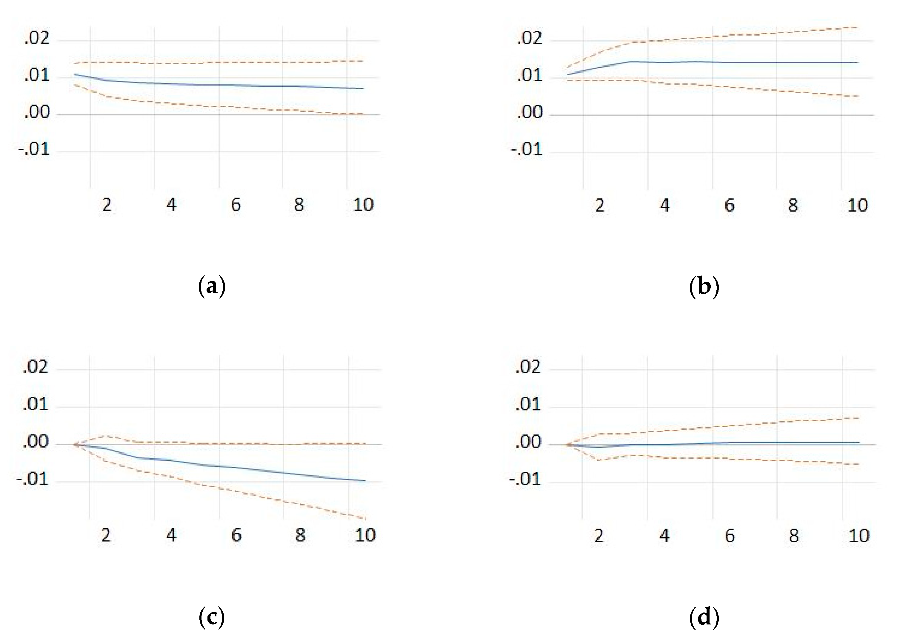
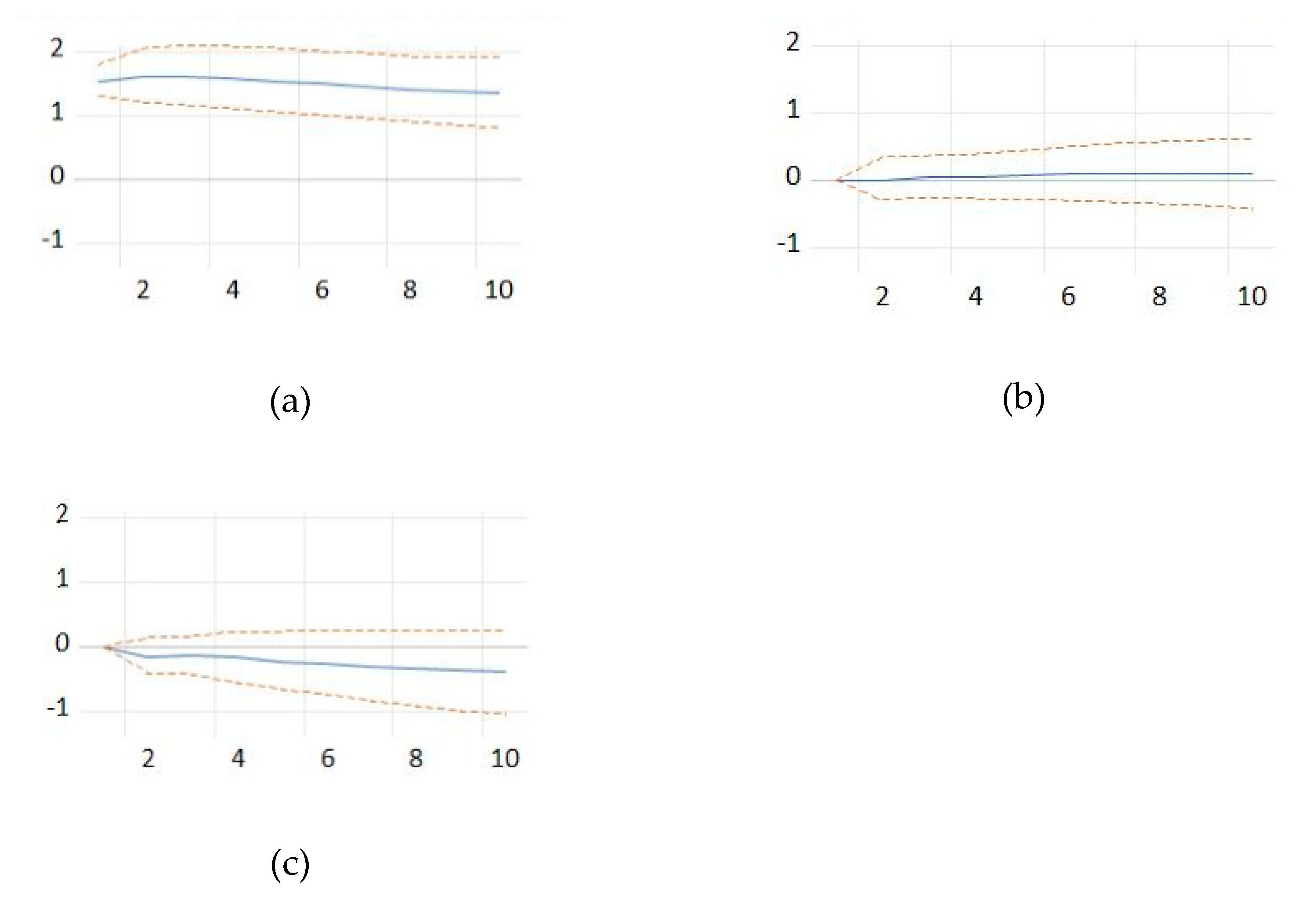
In the case of economic models, it is interesting to study the interaction between variables, requiring consideration of the effects of changes in one variable on the other variables. VAR models allow the study of the relationships between variables or non-zero residues’ effects by analyzing the impulse response (Lütkepohl 2005), which allows the identification of structural shocks reflected in a correlation in the innovation terms in Equations (8) to (15). The number of periods for which the shock response was estimated was ten, with the data being annual. 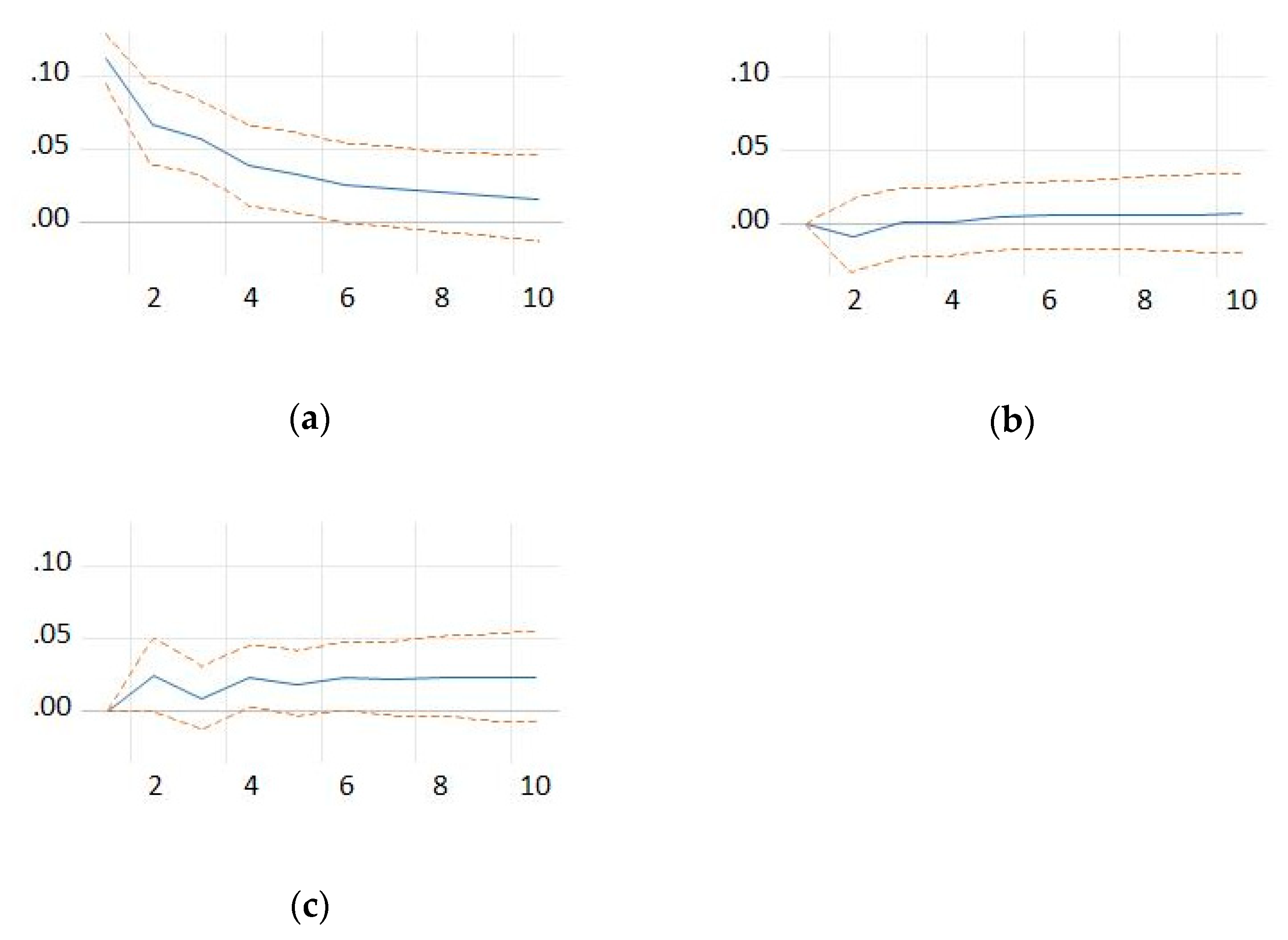The impulse responses for the long-run model are shown in Figure 3, Figure 4, Figure 5, Figure 6, Figure 7, Figure 8, Figure 9 and Figure 10. The definition of pulses used Cholesky decomposition, which considers the ordering of variables if they are correlated with each other. Looking at the VAR model coefficients, some interesting conclusions can be highlighted. Equation (8) means that the labor productivity per person is reacting in the next year to a shock at the level of GDP per capita, labor productivity per person, number of persons employed in the population of deaths and number of persons employed in the active enterprises in the following year (Figure 3). Remarkable is the decrease in the labor productivity per person when the number of persons employed in the population of deaths has a positive shock. This result is consistent with Landman’s empirical observations the short-term fluctuations of productivity and employment are strongly and positively correlated (2002).

Equation (9) shows how the GDP per capita is responding to a shock at the level of the GDP per capita, number of persons employed in the active enterprises and number of persons employed in the population of births in the previous year (Figure 4). It is remarkable that GDP per capita decreases in response to the shock of the number of persons employed in the population of births. This behavior could suggest that employees have a low level of pay at the beginning of the company’s activity. This result is also in line with previous studies (Molendowski and Żmuda 2013).

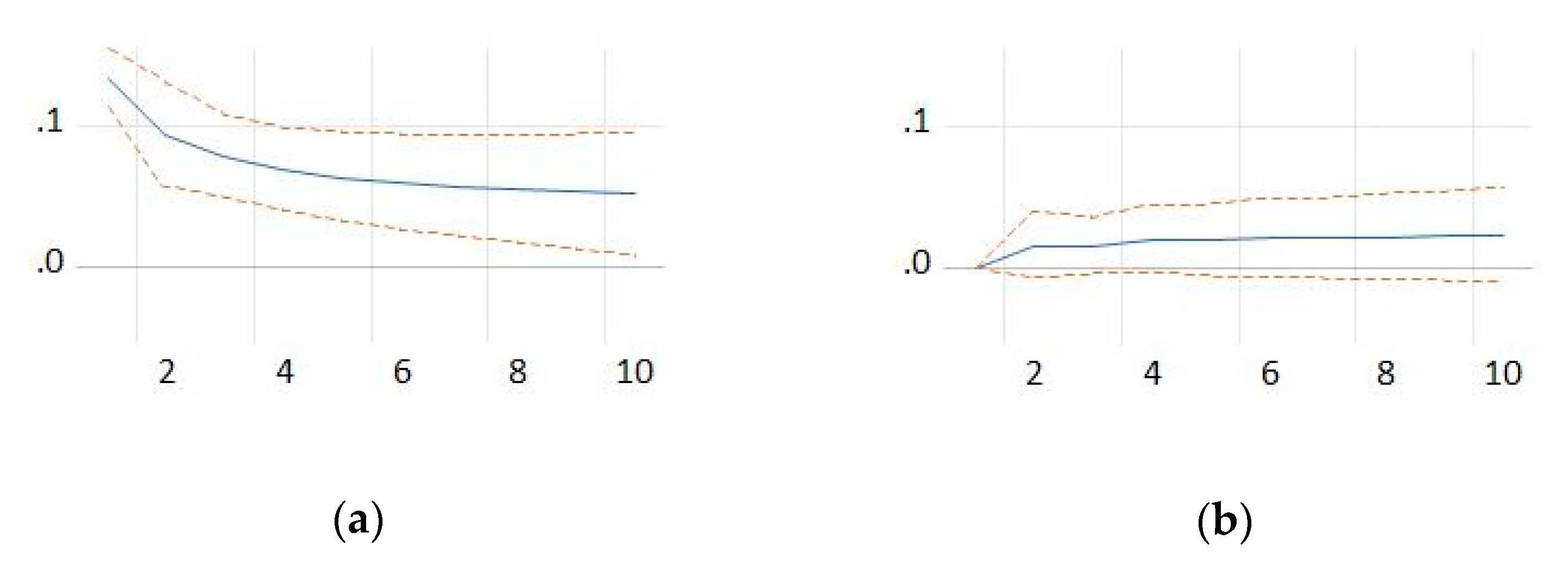
Equation (10) shows what the population of the active enterprises’ response looks like when there is a shock given in the number of persons employed in the population of newborn enterprises, the number of persons who were employed in the dead enterprises or the number of active enterprises in the previous year. The response of the population of active enterprises to a shock from the number of persons employed in births is the opposite to that of a shock from the number of persons employed in the population of deaths. (Figure 5).

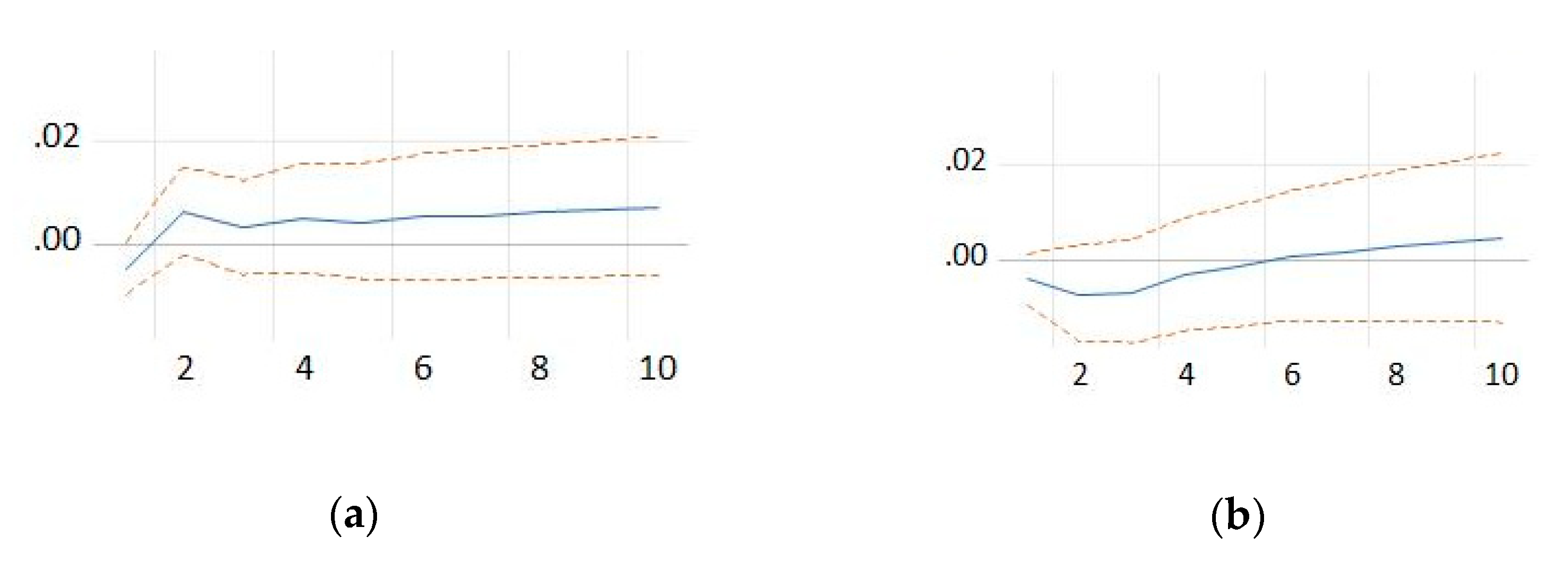
Equation (11) expresses the response of the births of enterprises to a shock from births of enterprises, nominal labor productivity per person and persons employed in the population of deaths in the previous year (Figure 6).

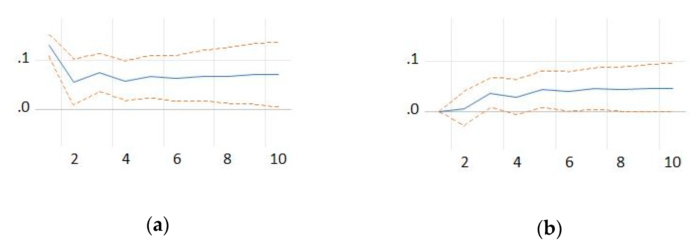
Equation (12) signifies that a shock at the level of the population of dead enterprises and the number of persons employed in the population of newborn enterprises generates effects on deaths of enterprises in the previous year (Figure 7).

Equation (13) shows that when a shock is given to the number of persons employed in the population of active enterprises, it generates effects at the level of the number of persons employed in the population of active enterprises in the following year (Figure 8).

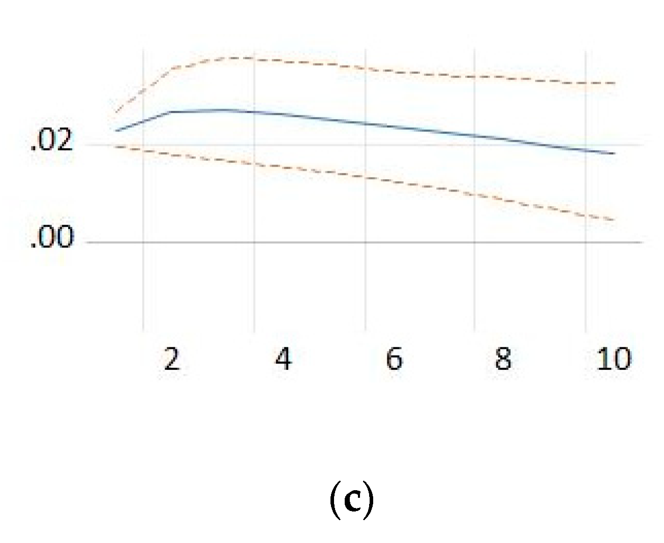
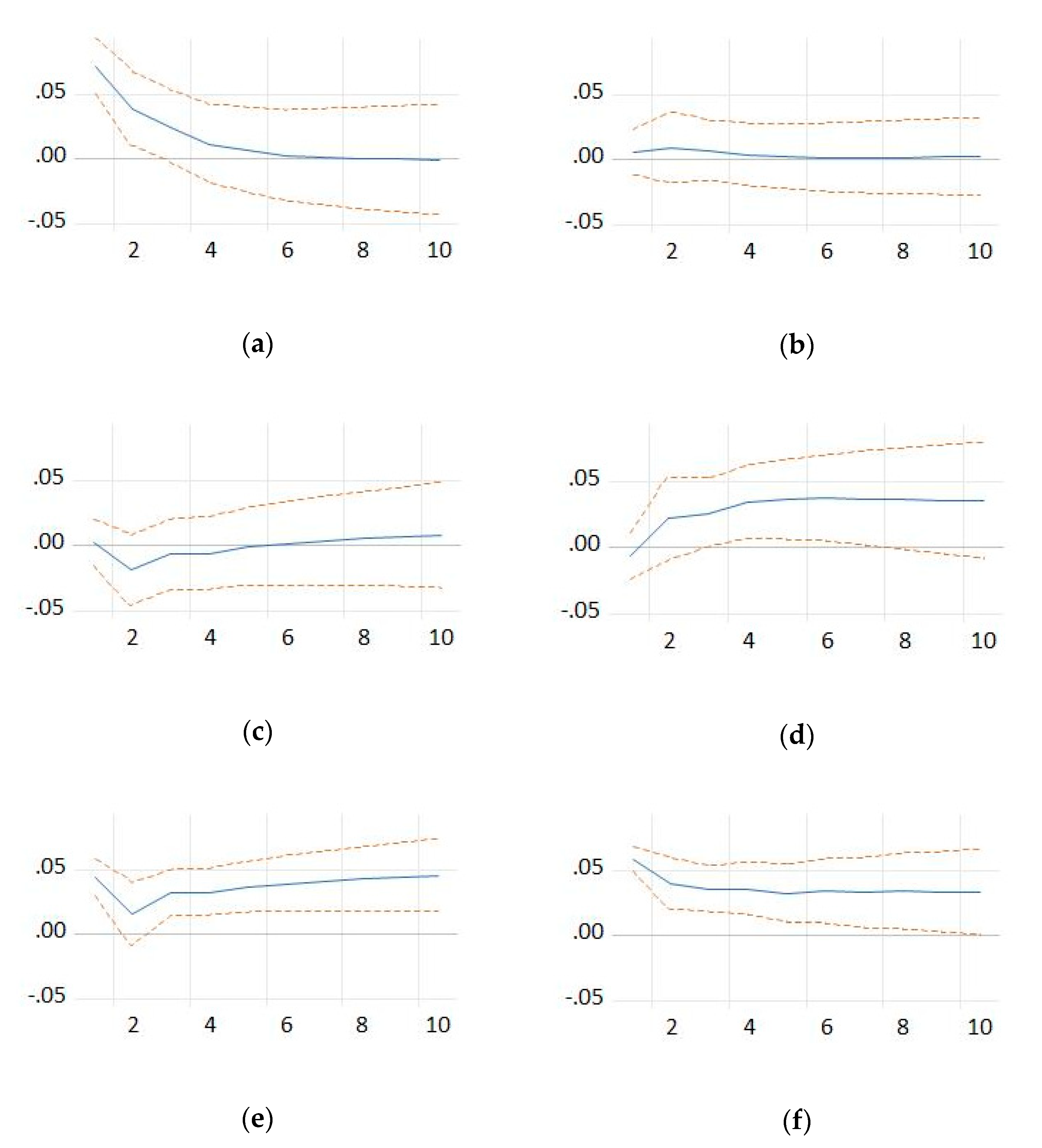
Equation (14) shows how a shock at the level of the number of persons employed in the population of dead enterprises and the number of persons employed in the population of newborn enterprises affects the number of persons employed in the population of dead enterprises in the following year (Figure 9).

Equation (15) expresses how the number of persons employed in the population of newborn enterprises will be affected in the following year by a shock at the level of the population of newborn enterprises or at the level of GDP per capita, the labor productivity per person, the number of persons employed in the population of dead enterprises, the number of persons employed in the population of active enterprises and the number of persons employed in the population of newborn enterprises in the previous year (Figure 10).

3.5. The VEC Model

When the analyzed variables are cointegrated, a VEC model can be constructed. Since the variables are not stationary (I (1)) and are not cointegrated, we first differentiated the variables, and we estimated the variables in the first differences of the variables. Constraints are introduced in the VEC model to allow long-term and short-term dynamic examination of the cointegrated series. In the case of studying economic relationships that are correlated and show long-term and short-term relationships, VEC models enable the separation of long-term and short-term components (Wooldridge 2008) (Asteriou and Hall 2016) (Hill et al. 2018).

In this line, as it is substantiated in literature (Asteriou and Hall 2016) (Wooldridge 2008) the VEC model is a representation of cointegrated VAR (courtesy of Granger’s representation theorem) and the resulting VAR from the VEC model representation has more efficient coefficient estimates. From this perspective, the VECM representation has several advantages: it reduces the effect of multicollinearity, long-term information is synthesized in matrix form, a more intuitive interpretation of the coefficients is obtained (capturing the long-term and short-term effects) and it is an adequate representation when changes of the previous period are of interest.

The cointegrated equation and long-run model are

$$\begin{gathered} EC{T}_{t-1}=1.000\ast lab\_pro{d}_{t-1}-0.0067\ast gdp\_per\_ca{p}_{t-1}+0.0484\ast \\ act\_en{t}_{t-1}+1.1884\ast birth\_en{t}_{t-1}-1.6718\ast death\_en{t}_{t-1}+0.5874\ast \\ pers\_emp\_act\_en{t}_{t-1}-2.3429\ast pers\_emp\_birth{s}_{t-1}+2.0242\ast \\ pers\_emp\_death{s}_{t-1}-4.4391 \end{gathered}$$

(16)

Equation (16) is the error correction equation and it signifies the long-run relationship among the variables. $EC{T}_{t-1}$ is the lagged value of the residuals obtained from the cointegrated regression of the dependent variable of the regressors. It contains long-run information derived from the long-run cointegrating relationship. In the analyzed dataset, the labor productivity shows a negative (−) association with GDP per capita, number of dead enterprises and number of persons employed in newborn enterprises. A positive (+) association appears with number of active enterprises, number of newborn enterprises, number of persons employed in active enterprises and number of persons employed in dead enterprises. As the variables are in logarithms, the coefficients can be interpreted as long-run elasticities. The result of Equation (16) as shown above is found to be questionable in terms of the labor productivity that has a negative sign with the GDP per capita relationship. This result is not in line with economic theory, suggesting the need to consider other variables in addition to modeling.

Table 12. Estimation of error correction term in the VEC model.

Variable	ECT Coefficients (t-Statistic)	Speed of Adjustment (t-Statistic)	Lag Coefficient (t-Statistic)	F-Statistic
lab_prod	1	−0.01378 (−3.25302)	0.001733 (0.90563)	2.717034
gdp_per_cap	0.048443 (−1.49061)	−0.8683 (−2.08262)	0.001771 (0.00941)	1.342875
act_ent	0.048443 (0.14168)	−0.01792 (−1.84941)	0.017323 (3.95798)	2.534653
birth_ent	1.188371 (2.35409)	−0.03879 (−1.20989)	0.038301 (2.64467)	2.750748
death_ent	−1.671782 (−4.43037)	−0.01249 (−0.34268)	0.00295 (0.17929)	0.677071
pers_emp_act_ent	0.587372 (1.44475)	−0.01339 (−1.32709)	0.013835 (3.03652)	0.886605
pers_emp_births	−2.342906 (−4.18569)	0.021932 (0.70223)	0.012686 (0.89933)	1.345365
pers_emp_deaths	2.044242 (5.19942)	−0.09775 (−1.88484)	−0.02904 (−1.23967)	2.392577

The authors’ own computations.

shows the estimated error correction time in the VEC model. The short-run model is:

$$\begin{array}{ll}\hfill \Delta lab\_pro{d}_t=& -0.013782\ast EC{T}_{t-1}+0.2687\ast \Delta lab\_pro{d}_{t-1}-0.0017\\ & \ast \Delta gdp\_per\_ca{p}_{t-1}+0.0124\ast \Delta act\_en{t}_{t-1}-0.0048\\ & \ast \Delta birth\_en{t}_{t-1}-0.0091\ast \Delta death\_en{t}_{t-1}-0.182\\ & \ast \Delta pers\_emp\_ect\_en{t}_{t-1}-0.0258\ast \Delta pers\_emp\_birth{s}_{t-1}\\ & +0.0171\ast \Delta pers\_emp\_death{s}_{t-1}+0.0017\end{array}$$

(17)

$$\begin{gathered} \Delta gdp\_per\_ca{p}_t=-0.868299\ast EC{T}_{t-1}-6,5811\ast \Delta lab\_pro{d}_{t-1}+ \\ 0.2048\Delta gdp\_per\_ca{p}_{t-1}+5.6755\ast \Delta act\_en{t}_{t-1}+0.0077\ast \\ \Delta birth\_en{t}_{t-1}-1,6245\ast \Delta death\_en{t}_{t-1}-0.2058\ast \\ \Delta pers\_emp\_ect\_en{t}_{t-1}-2,1794\ast \Delta pers\_emp\_birth{s}_{t-1}+1.6709\ast \\ \Delta pers\_emp\_death{s}_{t-1}+0.0018 \end{gathered}$$

(18)

$$\begin{array}{ll}\hfill \Delta act\_en{t}_t=& -0.017921\ast EC{T}_{t-1}-0.3128\ast \Delta lab\_pro{d}_{t-1}+0.0049\\ & \ast \Delta gdp\_per\_ca{p}_{t-1}+0.1775\ast \Delta act\_en{t}_{t-1}-0.1101\\ & \ast \Delta birth\_en{t}_{t-1}-0.0139\ast \Delta death\_en{t}_{t-1}-0.3657\\ & \ast \Delta pers\_emp\_ect\_en{t}_{t-1}+0.1704\ast \Delta pers\_emp\_birth{s}_{t-1}\\ & +0.0057\ast \Delta pers\_emp\_death{s}_{t-1}+0.0173\end{array}$$

(19)

$$\begin{array}{ll}\hfill \Delta birth\_en{t}_t=& -0.038794\ast EC{T}_{t-1}-0.6862\ast \Delta lab\_pro{d}_{t-1}+0.0151\\ & \ast \Delta gdp\_per\_ca{p}_{t-1}-0.3615\ast \Delta act\_en{t}_{t-1}-0.3015\\ & \ast \Delta birth\_en{t}_{t-1}-0.1406\ast \Delta death\_en{t}_{t-1}-1.0801\\ & \ast \Delta pers\_emp\_ect\_en{t}_{t-1}+0.4024\ast \Delta pers\_emp\_birth{s}_{t-1}\\ & +0.2579\ast \Delta pers\_emp\_death{s}_{t-1}+0.0383\end{array}$$

(20)

$$\begin{array}{ll}\hfill \Delta death\_en{t}_t=& -0.012485\ast EC{T}_{t-1}+0.4244\ast \Delta lab\_pro{d}_{t-1}+0.0007\\ & \ast \Delta gdp\_per\_ca{p}_{t-1}+0.8854\ast \Delta act\_en{t}_{t-1}-0.3547\\ & \ast \Delta birth\_en{t}_{t-1}-0.0904\ast \Delta death\_en{t}_{t-1}-0.2827\\ & \ast \Delta pers\_emp\_ect\_en{t}_{t-1}+0.1312\ast \Delta pers\_emp\_birth{s}_{t-1}\\ & -0.0464\ast \Delta pers\_emp\_death{s}_{t-1}+0.0030\end{array}$$

(21)

$$\begin{array}{l}\hfill \Delta pers\_emp\_ect\_en{t}_t\\ & =-0.013388\text{*}EC{T}_{t-1}-0.5833\ast \Delta lab\_pro{d}_{t-1}+0.0085\\ & \ast \Delta gdp\_per\_ca{p}_{t-1}-0.0271\ast \Delta act\_en{t}_{t-1}+0.0158\\ & \ast \Delta birth\_en{t}_{t-1}-0.0134\ast \Delta death\_en{t}_{t-1}-0.0815\\ & \ast \Delta pers\_emp\_ect\_en{t}_{t-1}+0.0139\ast \Delta pers\_emp\_birth{s}_{t-1}\\ & +0.0361\ast \Delta pers\_emp\_death{s}_{t-1}+0.0138\end{array}$$

(22)

$$\begin{array}{l}\hfill \Delta pers\_emp\_birth{s}_t\\ & =0.021932\ast EC{T}_{t-1}-1,4235\ast \Delta la{b}_{prod}{}_{t-1}+0.0195\\ & \ast \Delta gdp\_per\_ca{p}_{t-1}-0.4728\ast \Delta act\_en{t}_{t-1}+0.1873\\ & \ast \Delta birth\_en{t}_{t-1}-0.0876\ast \Delta death\_en{t}_{t-1}-0.5217\\ & \ast \Delta pers\_emp\_ect\_en{t}_{t-1}-0.1448\ast \Delta pers\_emp\_birth{s}_{t-1}\\ & +0.1504\ast \Delta pers\_emp\_death{s}_{t-1}+0.0127\end{array}$$

(23)

$$\begin{array}{l}\hfill \Delta pers\_emp\_death{s}_t\\ & =-0.097747\ast EC{T}_{t-1}+1,1390\ast \Delta lab\_pro{d}_{t-1}-0.0108\\ & \ast \Delta gdp\_per\_ca{p}_{t-1}+0.8070\ast \Delta act\_en{t}_{t-1}+0.0482\\ & \ast \Delta birth\_en{t}_{t-1}+0.3104\ast \Delta death\_en{t}_{t-1}+0.2821\\ & \ast \Delta pers\_emp\_ect\_en{t}_{t-1}-0.1887\ast \Delta pers\_emp\_birth{s}_{t-1}\\ & -0.3895\ast \Delta pers\_emp\_death{s}_{t-1}-0.0290\end{array}$$

(24)

In the case of the $\Delta lab\_prod$ estimation, the adjustment coefficient value is −0.013782. It measures the speed at which Y returns to equilibrium after changes in X and R. The interpretation of this value is that the previous years’ deviation from long-run equilibrium is corrected in the current period at a speed of 0.14 percent. For the GDP per capita coefficient, the percentage change is associated with a 0.17% decrease in labor productivity, the other conditions remaining, on average, unchanged in the short run. For the active enterprises number coefficient, the percentage change is associated with a 0.01% increase in labor productivity, the other conditions remaining, on average, unchanged in the short run. For the births of new enterprises number coefficient, the percentage change is associated with a 0.005% decrease in labor productivity, the other conditions remaining, on average, unchanged in the short run. For the dead enterprises number coefficient, the percentage change is associated with a 0.009% decrease in labor productivity, the other conditions remaining, on average, unchanged in the short run. For the number of persons employed in active enterprises coefficient, the percentage change is associated with a 0.18% decrease in labor productivity, the other conditions remaining, on average, unchanged in the short run. For the number of persons employed in births coefficient, the percentage change is associated with a 0.026% decrease in labor productivity, the other conditions remaining, on average, unchanged in the short run. For the number of persons employed in deaths coefficient, the percentage change is associated with a 0.17% increase in labor productivity, the other conditions remaining, on average, unchanged in the short run.

The high value of the adjustment coefficient, which is observed in the case of birth_ent, death_ent, pers_emp_births and pers_emp_deaths, indicates a rapid adjustment of the imbalance in the case of these variables, while the other coefficients act more slowly.

4. Discussions

The significant results in the VEC model highlight different situations of the variables considered. Thus, positive values that tend to zero indicate that the long-term adjustment process is slow; this is the case for GDP per capita and population of active enterprises. In the long run, births of enterprises, persons employed in the population of active companies and persons employed in the population of deaths show positive coefficients, which express that the action of these variables is toward a deflection of the equilibrium of labor productivity per person. In the case of deaths of enterprises and persons employed in the population of births, the negative values of the coefficients show that these variables act as factors that tend to overshoot the considered system from the long-run equilibrium path.

We analyzed whether the effects of the business demography variables on SMEs’ future economic performance are different according to the socio-economic model. Suppose countries increase their firms’ labor productivity by stimulation and development of entrepreneurship due to an improved socio-economic framework. In that case, it can be predicted that the increase in productivity will continue for an extended period. However, if GDP per capita increases, it is not expected that labor productivity will continue to grow in the next period as the impulse response function (IRF) show.

As it has been presented above, recent research addressed the issues of how the different models cope with the new challenges of the socio-economic environment (Aiginger 2008) (Aiginger and Guger 2005) (Esping-Andersen 1990) (Guger et al. 2007) and what we can learn from the evolutions and approach of each model. Given that the differences in economic performance between European countries increased in the 1990s, especially in terms of production dynamics, productivity and employment, most of these scientific contributions examine differences in performance between European countries, seeking to identify the factors growth and key areas for adaptability to present and future challenges. The evolution of society, determined especially by the unprecedented pace of progress, generates changes, both internally and externally. These changes, driven by the technological environment, include international competition, demographic aging, migration and the disintegration of traditional family structures, generating new risks for the individual and society as a whole, which requires European welfare states to adapt. These studies explore the differences in economic and social performance between European models to find the success factors of different strategic models for Europe.

In these studies, performed by data panel methods, the used datasets represent a small number of countries, divided into groups, depending on economic development, geographical location or other criteria. The grouping based on specific criteria was the factor that led to homogeneous characteristics within the respective groups. As presented in the previous paragraph, the use of data panel analysis methods only allows the control of heterogeneity. Despite the homogeneity of policy at the level of the European Union, regarding the status of development, there are still important disparities between groups, but also between countries belonging to the same group.

As we have shown above, the methods of analysis of the data panel were chosen because they allow the control of heterogeneity. Although cohesion has been an essential objective of European Union policies, fundamental differences remain between groups representing different development models and countries belonging to the same group. The availability of data on the 12 member states of the European Union that form the research panel is conditional on accession, which imposed a limitation of the period analyzed. All these countries have joined the Eurostat reporting framework, but they have the choice to use Eurostat databases taking into account the common reporting framework of the EU member states. Econometrically, this ensures the variables’ compatibility across the considered countries.

This research aimed to identify driving factors to enhance economic performances of firms, enabling the development of a common framework for EU economic policies. Our panel consists of 12 countries which are members of the European Union. The socio-economic diversity of the EU was taken into account, all European socio-economic models being represented at the panel level. All the nominalized countries have already adhered to the Eurostat reporting framework, but despite this, the availability of data related to them is limited compared to the moment of joining. Choosing to use the Eurostat data is based on their compatibility along with the panel countries. The dynamic VEC model can be used to generate predictions to analyze the impact of random perturbations (shocks) on the system variables. It can be concluded that analyzed variables need to be the set of analyzed variables that must be completed with other variables. On the other hand, the subject is of real interest and needs to be resumed in the future, as new data will be valid to represent all EU countries. Analyzing the evolution of nominal labor productivity per person values, at the level of all countries representing the socio-economic models considered, it is clear that this generates more important effects in more developed economies. The countries belonging to the Catching-up model and, especially, Bulgaria and Romania show much lower influences at the level of this indicator. In the case of GDP per capita, countries are grouped differently. Thus, Denmark, Sweden, Germany and Belgium are the leading group. These are followed by the group formed by the UK, France, Italy and Spain, to which also the Czech Republic could be joined. In the last positions is the group formed by Hungary, Romania and Bulgaria. In terms of the population of active enterprises, the grouping of countries is quite surprising. Thus, in the group with the most dynamic enterprises are Italy, France, Germany, Spain and the UK. These are followed by the group formed by the Czech Republic, Sweden, Belgium, Hungary and Romania. In the last positions is the group formed by Bulgaria and Denmark. In terms of births of enterprises, in essence, the countries are grouped into two clusters. Thus, France, Italy, Germany, Spain and the UK are at the forefront of higher values of this indicator. The other countries, namely, the Czech Republic, Romania, Hungary, Sweden, Bulgaria, Belgium and Denmark, showed relatively low values of the number of newborn enterprises. Regarding the deaths of enterprises, the countries could be grouped somewhat similarly, with the observation that, in the second group, the hierarchy is slightly changed. The same grouping was highlighted in the case of the number of persons employed in active enterprises, and also in the case of the number of persons employed in births, with the observation that Denmark, ranked last, distanced itself from the other six countries. In the case of the number of persons employed in death, two countries stand out from the second group, namely, Belgium and Denmark, which had the lowest values for this indicator.

The surprise is that the reforms are going in the same direction, mostly independent of the starting model. A general European model could represent a competitive advantage in an increasingly competitive environment, allowing the EU to become a high-performing region as a whole. The new changes transform globalization from a downward race to a top race, implementing future strengths such as innovation, education, lifelong learning and new technologies. The construction of functional economic models with a high degree of economic efficiency involves, at the EU level, the capitalization of local specificities, the development of key economic sectors, the promotion of technological progress and related developments. The role of the SME sector in stimulating and promoting economic growth is a vital one with wide influences in the European Union. The significant potential of SMEs lies not only in the ability to provide products and services with a high degree of competitiveness and functionality in the economy, but also, especially, in the ability to mobilize the factors and production resources available at the EU level.

From this perspective, the European Union’s strategy for the period 2021–2027 envisages a more personalized approach to regional development. It further seeks to eliminate the shortcomings of our development model and create favorable conditions for reducing disparities within the European Union. Cohesion policy continues to invest in all regions, based on three categories, namely, less developed regions; transition regions; and more developed regions. The outermost regions will continue to receive special support from the EU. The method of funds allocation is still based mainly on GDP per capita.

5. Conclusions

The main contribution of the paper is the analysis on the evolution, concentration, framing and assessment of belonging of a country or group of countries to an economic model already defined in the literature, from the perspective of SME specific indicators and their influence on labor productivity. The goal was to understand the process by which national economies with different levels of development can group and form a viable economic model within the European one, but also the process of catching up and achieving the degree of convergence with the EU average of those that register gaps, following a faster growth path through the SME sector, aiming both to make the EU compatible with global developments and to harmonize the new members. Therefore, a significant challenge for the Eastern European countries (Romania and Bulgaria) is the harmonization of economic and social standards at the EU level, a knowledge-based challenge. The question is whether there is an appropriate economic and social development model for these countries (Romania and Bulgaria), which could help reduce the gaps as quickly as possible. In our opinion, the differences among regions could reflect specific conditions. Identifying these conditions could be used to substantiate development policies. The multitude of existing economic models is in line with the European economic and social model, being able to provide a high degree of convergence. In this context, a connection between European socio-economic models and the SMEs’ performance is revealed.

Nordic countries are considered some of the best worldwide. In 2009, Sweden’s nominal labor productivity per person was higher than that of Denmark. Noteworthy is the fact that, starting in 2010, Denmark began to close the gap, so that, since in 2016, the hierarchy reversed, this trend was continued in 2017. The UK represents the Anglo-Saxon model. The nominal labor productivity per person started to decrease from 2013, with this trend maintained until the end of the analyzed period. Belgium, France and Germany represent the Continental model. Of these, Belgium stands out in terms of the nominal labor productivity per person, and France is ahead of Germany. Czech Republic and Hungary are identified in the Catching-up model. They joined the European Union in 2004. At that time, they were considered relatively undeveloped economies, but showing a significant potential. Romania and Bulgaria are ranked in the last places.

The industrial transition and the changing European economic paradigm generate an additional set of challenges for SMEs. Improving the level of labor force quality, increasing the degree of endowment with capital and modernizing and adapting the industrial base emphasize the need for reforms of existing redistributive systems at the community level.

Modernizing the EU economic system in line with the objectives of this new cycle is necessary to ensure both social cohesion and strengthening the competitiveness of the European model.. The structural changes of the economy and the forms of business organization have an essential role in the industrial transition and the development of new forms and models of socio-economic development. The involvement of the state governments through specific public policies has strengthened the traditional economic models, and the development of the SME sector and entrepreneurship have been aligned with these requirements, although in some places they have generated significant changes in local economic structures.

Research Limits

This paper’s most significant limitation is that the variables considered were not available for the specified period for all EU countries. This lack of data was the major limitation. For this reason, only data for 2009–2017 were analyzed because the data series for 2018 were not yet available for all variables and countries. These considerations have made it impossible to carry out an analysis for all EU countries. Another limitation is that the variables used are not specific to SMEs, being relative to enterprises, in general.