
Central Counterparties and Liquidity Provision in Cash Markets

Abstract
:Balance sheet space is treated like expensive real estate, available only to positions that can afford to pay rental fees that are now much higher.Darrell Duffie in Forbes, 11 March 2016
1. Introduction
2. Institutional Background
2.1. Basel III Leverage Rule and Market Making
2.2. Trading on the MTS Platform
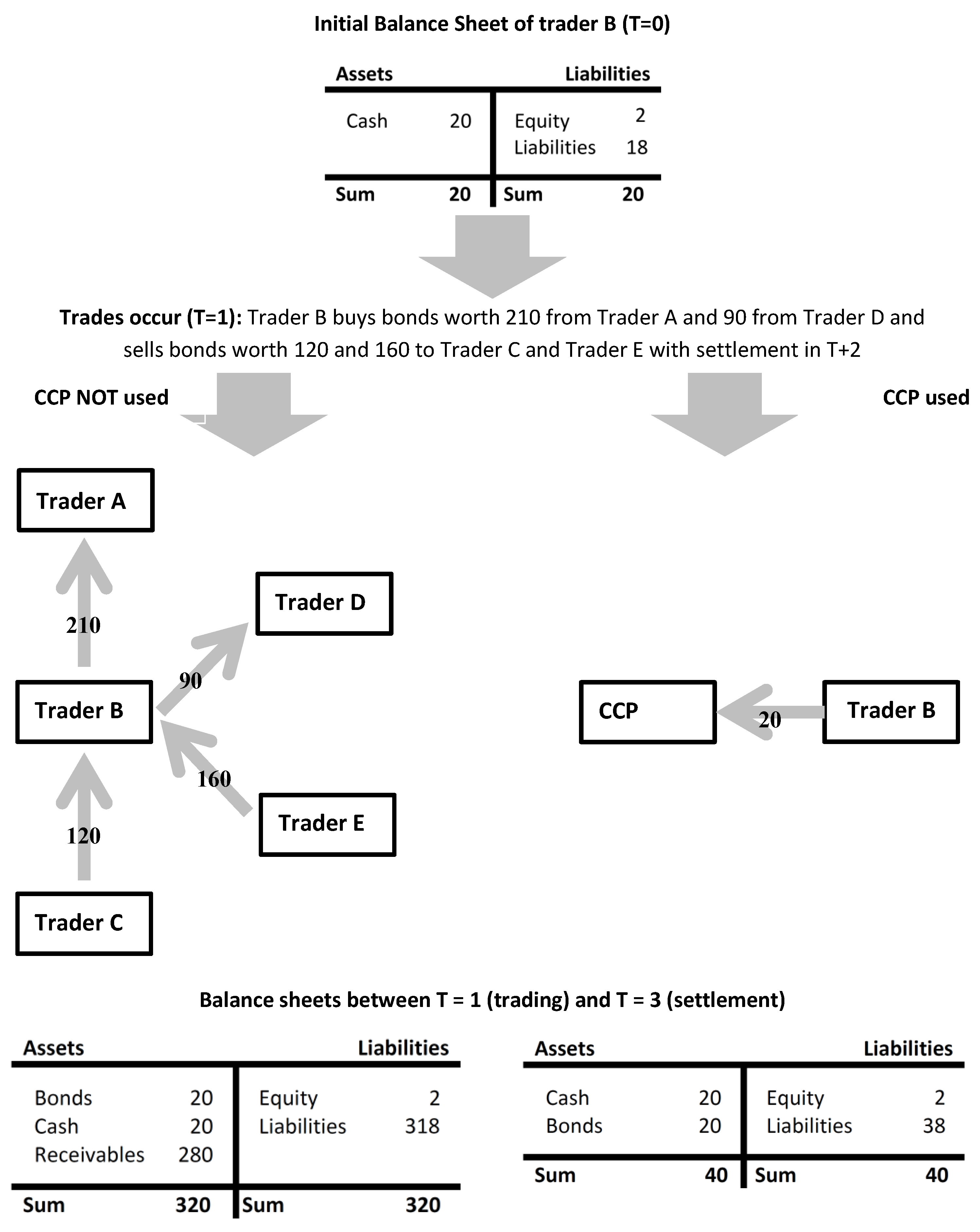
2.3. Balance Sheet Effects of Central Counterparties
3. Data
4. Variables and Descriptive Statistics
4.1. Trading Activity
4.2. Liquidity
4.3. Control Variables
5. Empirical Analysis
5.1. Trading Activity
5.2. Liquidity
6. Robustness
6.1. Placebo Test
6.2. Zero-Trading Days
6.3. Window Dressing
6.4. Country Groups
7. Conclusions, Limitations and Outlook
Funding
Institutional Review Board Statement
Informed Consent Statement
Data Availability Statement
Conflicts of Interest
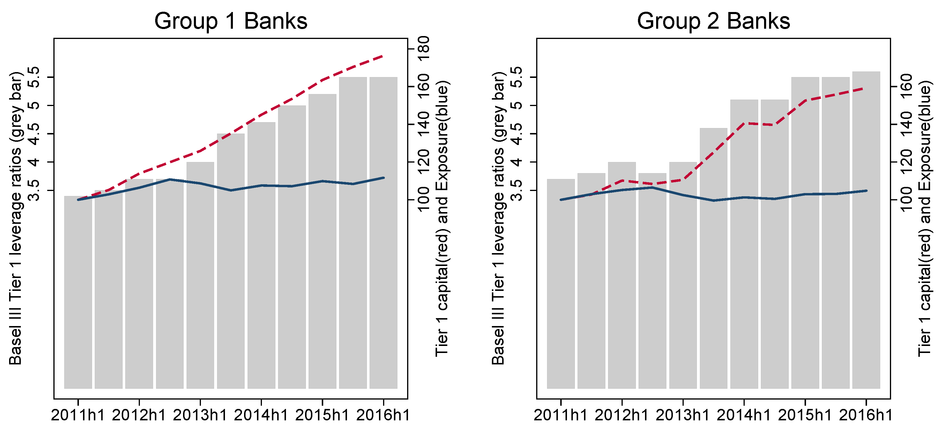
| 1 | The regulation set a target leverage ratio of 3% for a trial period between 2013 and 2017. This target ratio was not immediately a binding minimum capital requirement (Pillar 1). However, it was immediately part of the supervisory review of banks (Pillar 2) and disclosure requirements (Pillar 3). Moreover, the leverage ratio became a binding capital requirement (Pillar 1) in 2018 (PWC (2018)). As can be seen from Figure 1, the adoption of the rule into law and the anticipation that it would become a part of Pillar 1 led to a significant decrease in bank leverage. This is consistent with Committee on the Global Financial System (2016), whose survey results revealed that banks were already estimating current regulatory costs according to fully phased-in Basel III, which indicates that the adjustment of business models had already taken place. |
| 2 | See Section 2.3 and Table 1 for more details on the settlement infrastructure of the MTS platform. |
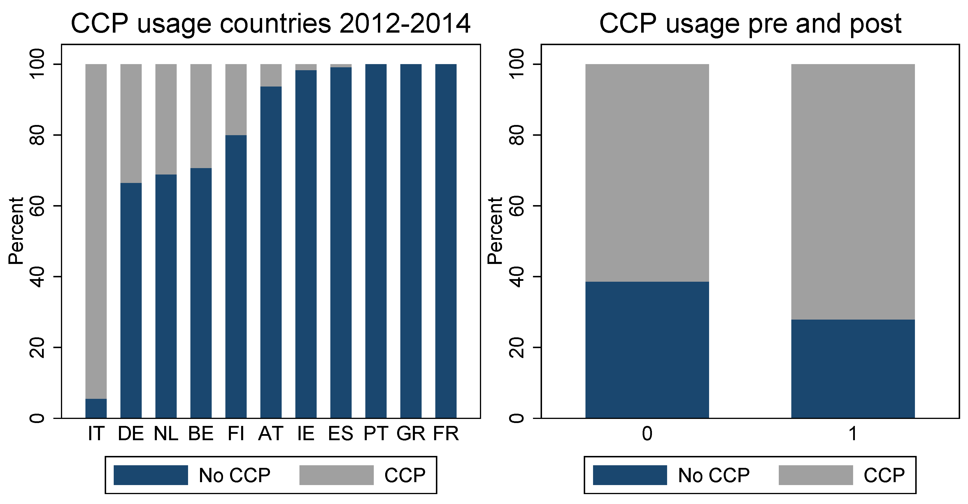
| 3 | CCPs have become increasingly important in cash markets. In 2015, bond trades worth more than 66 trillion were routed via the three largest CCPs in Europe. (The ECB names LCH.Clearnet SA, LCH.Clearnet Ltd. and EUREX Clearing AG as the biggest CCPs according to the number of participants.) On MTS, more than 60% of the trades were executed via CCPs. |
| 4 | |
| 5 | |
| 6 | The 2013 document was termed: “Consultative Document Revised Basel III leverage ratio framework and disclosure requirements”. |
| 7 | Due to interoperability arrangements, dealers in the Italian market can either be a CC&G or LCH.Clearnet SA member because the two institutions form a single virtual CCP (each CCP is a member of the other CCP). For further information, consult: https://www.bancaditalia.it/compiti/sispaga-mercati/controparte-centrale (accessed on 1 September 2017). |
| 8 | Further information on membership eligibility can be found at: https://www.lch.com/membership (accessed on 1 November 2017). |
| 9 | The MTS Cash Domestic Market Rules (MTS (2017)) specify on p. 22: “If Quotes and Orders matching on the Market, are submitted by two Dealers using the CCP Services on a Financial Instrument eligible for CCP Service, the execution of the Trade shall be automatic subject to the registration of the Trade by the CCP, if the applicable CCP regulations provide that the novation of the relevant Trade shall take place upon the registration of the Trade by the CCP”. |
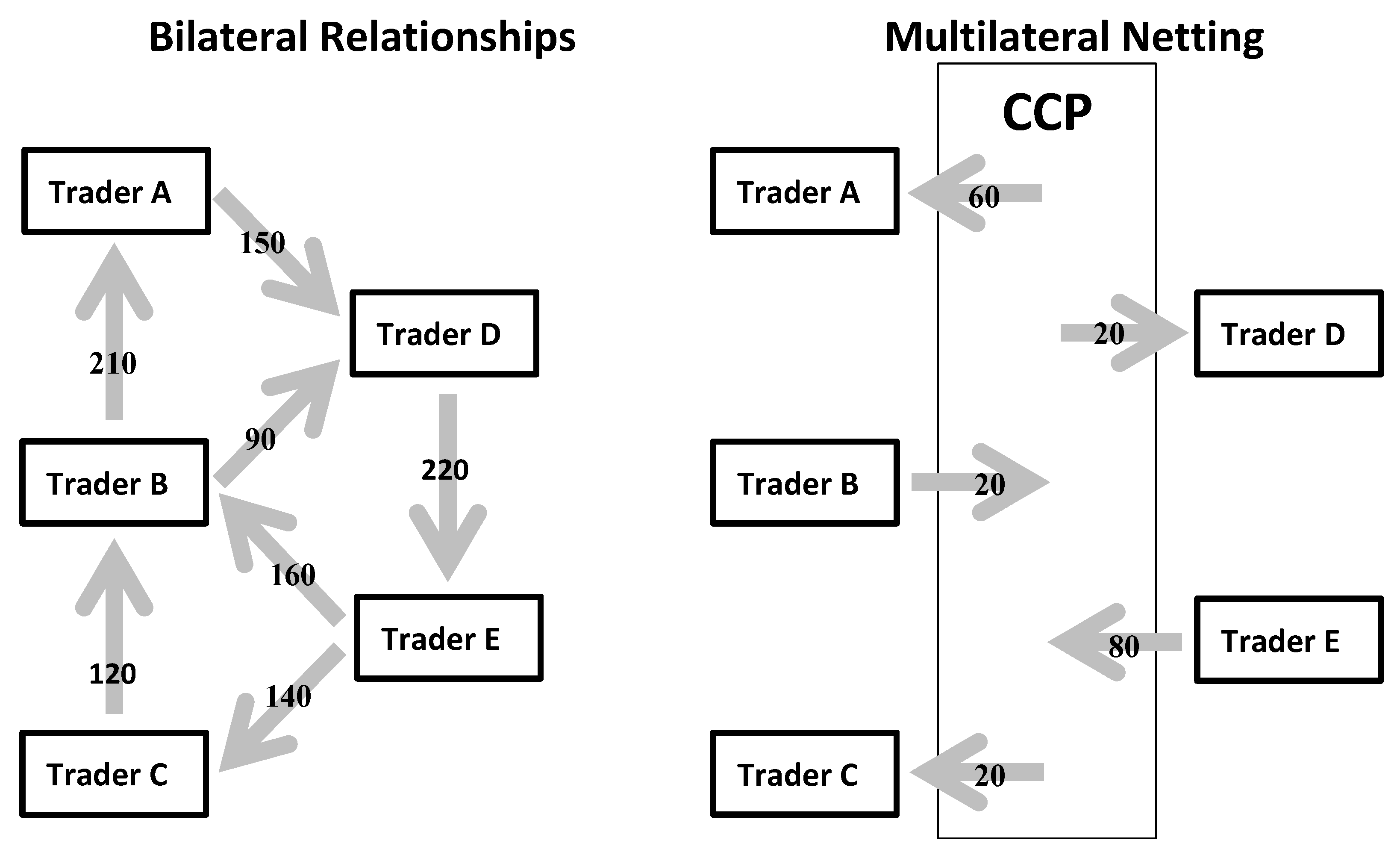
| 10 | According to the LCH Limited Procedures section 2B RepoClear clearing service (http://www.lch.com/rules-regulations/rulebooks/ltd (accessed on 1 September 2017), the netting process works as follows: (1) First, all delivery obligations are collected (for each settlement day and settlement system). (2) Next, contracts arising from (eligible) bond trades are netted by the CCP at the participant, security and settlement system levels. (3) Netting takes place every day and considers all (eligible) contracts for settlement on that day. (4) Finally, the netting process creates net delivery and receipt obligations (for securities and for cash) for each member, securities issue and settlement system combination. The procedures for the LCH SA work very similarly (see http://www.lch.com/rules-regulations/rulebooks/s (accessed on 1 September 2017) and CC&G http://www.lseg.com/node/5437 (accessed on 1 September 2017). |
| 11 | LCH. Limited (2017) states that “In such netting process no distinction will be made between securities forming part of RepoClear Contracts arising from RepoClear Repo Transactions, Repo Trades or Bond Trades”. |
| 12 | |
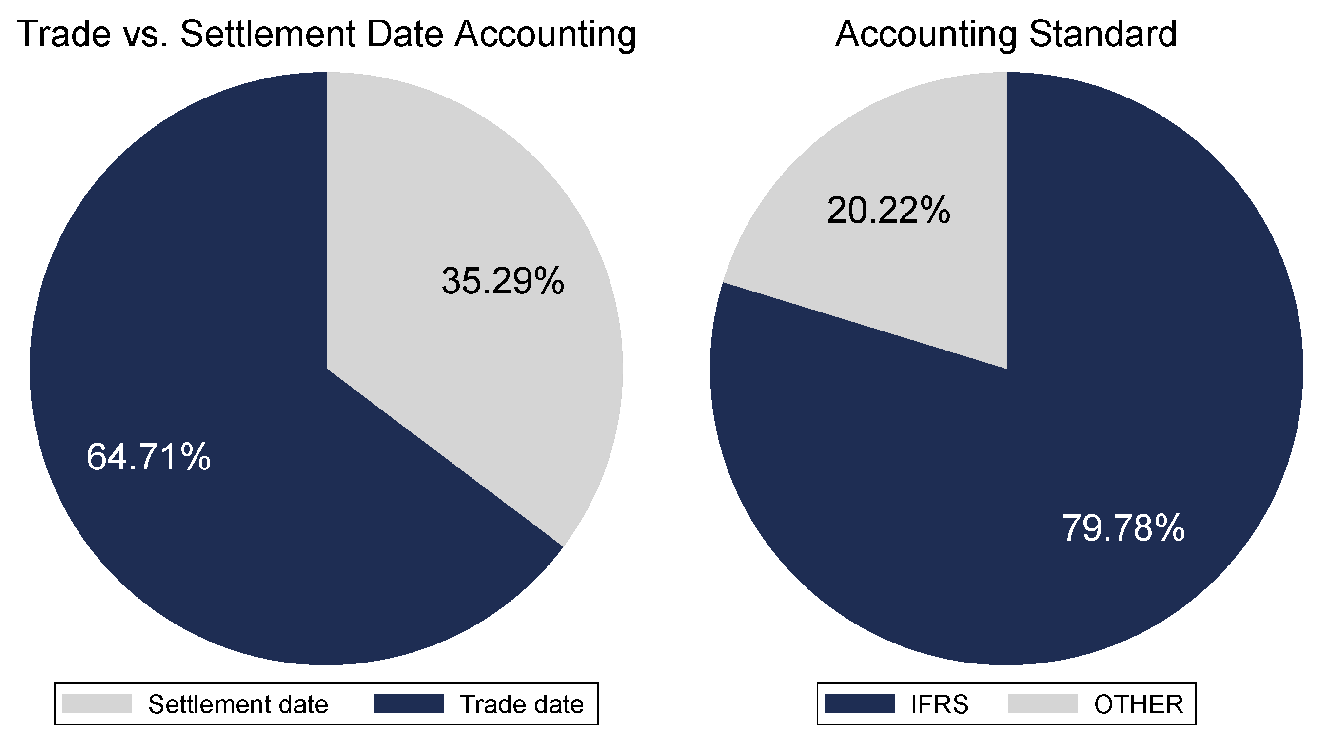
| 13 | Initially and during our entire sample period, the Basel III framework relied on accounting data to calculate the exposure arising from trade liabilities and receivables. However, in a finalized version of the Basel III framework (BCBS (2017b)), the BCBS recognized that different accounting standards (e.g., US Gaap and IFRS) and choices (settlement vs. trade date accounting) lead to different impacts of trading activity on the exposure measure. Thus, Basel III rules define a deviation from accounting standards for the purpose of calculating the exposure arising from trade payables and receivables. These rules specify that even if banks are allowed to net trade payables and receivables under their respective accounting standards, they are not allowed to do so for the purpose of calculating the Basel III leverage ratio. However, the regulation defines its own criteria for circumstances under which banks are allowed to net exposures. Note that these changes were not announced during our sample period. Their possibility was first mentioned in a consultative paper issued in 2016 (BCBS (2016)). |
| 14 | The receivables and liabilities remain in the balance sheet until the trade is settled. Currently, on MTS, the settlement date is T + 2 days from the trade date T (date on which the involved parties agree to exchange the bonds). |
| 15 | According to IAS 39 AG53, the chosen method has to be “applied consistently for all purchases and sales of financial assets that belong to the same category of financial assets”. Settlement date accounting seems to be the preferable method in the context of balance sheet exposures arising from unsettled trades described above but can be inferior to trade date accounting when it comes to hedging instruments (position appears in the balance sheet later) and non-regular way transactions (IAS 39 AG12), e.g., long settlement transactions (transaction has to be accounted as the derivative between the trade and settlement date). |
| 16 | A comprehensive explanation of the applied screens and error corrections can be found in Östberg and Richter (2017). |
| 17 | The distribution of bonds across countries is as follows: Austria 24, Belgium 191, Germany 157, Finland 18, Ireland 31, Italy 192 and The Netherlands 71. |
| 18 | The bond and trade characteristics that are associated with CCP usage and the way that market makers can use these variables to predict the likelihood of a CCP counterparty are discussed in detail in Section 5.2. |
| 19 | If the two groups exhibit diverging trends, the difference-in-difference coefficient may just capture this instead of differences between the two groups arising from the introduction of the Basel III leverage rule. |
| 20 | The rather weak results for the trading activity measures seem to be caused by unequally developed repo trading in different national MTS markets. As reported by Sigelman and Zeng (2000), banks significantly reduce repo trading at quarter-ends. Italy is the only market that has a big MTS repo market. Many cash trades are associated with repo trades (Duffie (1996)). Italy also has a high share of CCP trades. Thus, the reduction in repo trading might have more pronounced effects on the CCP trading activity and might act as a counterfactual. In an unreported analysis, we verified that the coefficient becomes significant in the and regressions when Italy is excluded. |
References
- Adrian, Tobias, Nina Boyarchenko, and Or Shachar. 2017. Dealer balance sheets and bond liquidity provision. Journal of Monetary Economics 89: 92–109. [Google Scholar] [CrossRef] [Green Version]
- Allen, Linda, and Anthony Saunders. 1992. Bank window dressing: Theory and evidence. Journal of Banking & Finance 16: 585–623. [Google Scholar]
- Anbil, Sriya, and Zeynep Senyuz. 2018. The Regulatory and Monetary Policy Nexus in the Repo Market. Available online: https://ssrn.com/abstract=3187697 (accessed on 3 December 2021).
- American Institute of Certified Public Accountants. 2017. Accounting Guide: Brokers and Dealers in Securities. Hoboken: John Wiley & Sons. [Google Scholar]
- Bank for International Settlements. 1992. Delivery versus Payment in Security Settlement Systems. Available online: http://www.bis.org/cpmi/publ/d06.pdf (accessed on 3 December 2021).
- Bao, Jack, Maureen O’Hara, and Xing Alex Zhou. 2016. The Volcker Rule and Market-Making in Times of Stress. Journal of Financial Economics. Forthcoming, Fourth Annual Conference on Financial Market Regulation. Available online: https://ssrn.com/abstract=2836714 (accessed on 3 December 2021).
- Basel Committee on Banking Supervision. 2017a. Basel III Monitoring Report. Available online: http://www.bis.org/bcbs/publ/d397.pdf (accessed on 3 December 2021).
- Basel Committee on Banking Supervision. 2017b. Basel III: Finalising Post-Crisis Reforms. Available online: https://www.bis.org/bcbs/publ/d424.htm (accessed on 3 December 2021).
- Basel Committee on Banking Supervision. 2010. Basel III: A Global Regulatory Framework for More Resilient Banks and Banking Systems. Available online: https://www.bis.org/publ/bcbs189.pdf (accessed on 3 December 2021).
- Basel Committee on Banking Supervision. 2013. Revised Basel III Leverage Ratio Framework and Disclosure Requirements—Consultative Document. Available online: https://www.bis.org/publ/bcbs251.pdf (accessed on 3 December 2021).
- Basel Committee on Banking Supervision. 2014. Basel III Leverage Ratio Framework and Disclosure Requirements. Available online: http://www.bis.org/publ/bcbs270.pdf (accessed on 3 December 2021).
- Basel Committee on Banking Supervision. 2016. Revisions to the Basel III Leverage Ratio Framework—Consultative Document. Available online: https://www.bis.org/bcbs/publ/d365.htm (accessed on 3 December 2021).
- Bellia, Mario, Roberto Panzica, Giulio Girardi, Loriana Pelizzon, and Tuomas A. Peltonen. 2018. The Demand for Central Clearing: To Clear or Not to Clear, That Is the Question. SAFE Working Paper No. 193. Frankfurt: Leibniz Institute for Financial Research SAFE. [Google Scholar]
- Bertrand, Marianne, Esther Duflo, and Sendhil Mullainathan. 2004. How much should we trust differences-in-differences estimates? The Quarterly Journal of Economics 119: 249–75. [Google Scholar] [CrossRef] [Green Version]
- Bessembinder, Hendrik, Stacey E. Jacobsen, William Maxwell, and Kumar Venkataraman. 2018. Capital commitment and illiquidity in corporate bonds. Journal of Finance 73: 1615–61. [Google Scholar] [CrossRef]
- Blum, Jürg M. 2008. Why Basel II may need a leverage ratio restriction. Journal of Banking & Finance 32: 1699–707. [Google Scholar]
- Boissel, Charles, Francois Derrien, Evren Ors, and David Thesmar. 2017. Systemic risk in clearing houses: Evidence from the European repo market. Journal of Financial Economics 125: 511–36. [Google Scholar] [CrossRef]
- Brunnermeier, Markus K. 2009. Deciphering the liquidity and credit crunch 2007–2008. The Journal of Economic Perspectives 23: 77–100. [Google Scholar] [CrossRef] [Green Version]
- Carhart, Mark M., Ron Kaniel, David K. Musto, and Adam V. Reed. 2002. Leaning for the tape: Evidence of gaming behavior in equity mutual funds. Journal of Finance 57: 661–93. [Google Scholar] [CrossRef] [Green Version]
- Comerton-Forde, Carole, Terrence Hendershott, Charles M. Jones, Pamela C. Moulton, and Mark S. Seasholes. 2010. Time Variation in Liquidity: The Role of Market Maker Inventories and Revenues. The Journal of Finance 65: 295–331. [Google Scholar] [CrossRef] [Green Version]
- Committee on Payments and Market Infrastructures. 2015. Statistics on Payment, Clearing and Settlement Systems in the CPMI Countries—Figures for 2015. Available online: http://www.bis.org/cpmi/publ/d155.htm (accessed on 3 December 2021).
- Committee on the Global Financial System. 2016. Fixed Income Market Liquidity. CGFS Papers No. 55. Basel: Bank for lInternational Settlements. [Google Scholar]
- Cont, Rama, and Thomas Kokholm. 2014. Central clearing of OTC derivatives: Bilateral vs. multilateral netting. Statistics & Risk Modeling l31: 3–22. [Google Scholar]
- Di Maggio, Marco. 2017. Comment on: Dealer Balance Sheets and Bond Liquidity Provision by Adrian, Boyarchenko and Shachar. Journal of Monetary Economics 89: 110–12. [Google Scholar] [CrossRef]
- Dunne, Peter G., Harald Hau, and M. Moore. 2010. A Tale of Two Platforms: Dealer Intermediation in the European Sovereign Bond Market. INSEAD Working Paper No. 2010/64/FIN. Paris: INSEAD. [Google Scholar]
- Duffie, Darrell. 2020. Still the World’s Safe Haven? Redesigning the US Treasury market after the COVID-19 crisis’. Hutchins Center on Fiscal and Monetary Policy at Brookings. Available online: https://www.brookings.edu/research/still-the-worlds-safe-haven (accessed on 28 November 2021).
- Duffie, Darrell. 1996. Special repo rates. The Journal of Finance 51: 493–526. [Google Scholar] [CrossRef]
- Duffie, Darrell. 2017. Financial regulatory reform after the crisis: An assessment. Mangement Science 64: 4835–57. [Google Scholar] [CrossRef] [Green Version]
- Dufour, Alfonso, Miriam Marra, and Ivan Sangiorgi. 2019. Determinants of intraday dynamics and collateral selection in centrally cleared and bilateral repos. Journal of Banking and Finance 107: 1–26. [Google Scholar] [CrossRef]
- Fleming, Michael J., and Frank M. Keane. 2021. The Netting Efficiencies of Marketwide Central Clearing. FRB of New York Staff Report No. 964. New York: Federal Reserve Bank of New York. [Google Scholar]
- Foucault, Thierry, Pagano Marco, and Alisa Röell. 2013. Market Liquidity: Theory, Evidence, and Policy. Oxford: Oxford University Press. [Google Scholar]
- Greene, William H. 2012. Econometric Analysis, 7th ed. London: Pearson Education. [Google Scholar]
- Haene, Philipp, and Andy Sturm. 2009. Optimal Central Counterparty Risk Management. Working Papers No. 2009-07. Bern: Swiss National Bank. [Google Scholar]
- Heckman, James J. 1981. The Incidental Parameters Problem and the Problem of Initial Conditions in Estimating a Discrete Time-Discrete Data Stochastic Process. Strutural Analysis of Discrete Data, S. 179–95. [Google Scholar]
- Ho, Thomas, and Hans R. Stoll. 1981. Optimal dealer pricing under transactions and return uncertainty. Journal of Financial Economics 9: 47–73. [Google Scholar] [CrossRef]
- Hu, Gang, David R. McLean, Jeffrey Pontiff, and Qinghai Wang. 2014. The year-end trading activities of institutional investors: Evidence from daily trades. The Review of Financial Studies 27: 1593–614. [Google Scholar] [CrossRef]
- Lakonishok, Josef, Andrei Shleifer, Richard Thaler, and Robert Vishny. 1991. Window dressing by pension fund managers. American Economic Review 81: 227–31. [Google Scholar]
- LCH. Limited. 2017. Procedures Section 2B RepoClear Clearing Service. Available online: https://www.lch.com/system/files/media_root/Section%202B%20-%20RepoClear%20Service.pdf (accessed on 20 December 2017).
- Loon, Yee C., and Zhaodong K. Zhong. 2014. The impact of central clearing on counterparty risk, liquidity, and trading: Evidence from the credit default swap market. Journal of Financial Economics 112: 91–115. [Google Scholar] [CrossRef]
- Mancini, Loriano, Angelo Ranaldo, and Jan Wrampelmeyer. 2015. The euro interbank repo market. The Review of Financial Studies 29: 1747–79. [Google Scholar] [CrossRef]
- Mendoza, Enrique G. 2010. Sudden stops, financial crises, and leverage. The American Economic Review 100: 1941–66. [Google Scholar] [CrossRef]
- Neyman, Jerzy, and Elizabeth L. Scott. 1948. Consistent estimates based on partially consistent observations. Econometrica 16: 1–32. [Google Scholar] [CrossRef]
- MTS. 2017. MTS Cash Domestic Rules. Available online: https://www.mtsmarkets.com/sites/default/files/content/documents/MTS%20Cash%20Domestic%20Market%20Rules%2014%2012%\202017%20clean.pdf (accessed on 30 December 2017).
- Östberg, Per, and Thomas Richter. 2017. The Sovereign Debt Crisis: Rebalancing or Freezes? Swiss Finance Institute Research Paper No. 17/32. Geneva: Swiss Finance Institute. [Google Scholar]
- O’Hara, Maureen, and Xing A. Zhou. 2021. The electronic evolution of corporate bond dealers. Journal of Financial Economics 140: 368–90. [Google Scholar] [CrossRef]
- PWC. 2018. Basel IV: The Leverage Ratio Revisited. Available online: https://www.pwc.co.uk/financial-services/assets/pdf/hot-topic-the-leverage-ratio.pdf (accessed on 1 February 2018).
- Sigelman, Lee, and Langche Zeng. 2000. Analyzing Censored and Sample-Selected Data with Tobit and Heckit Models. Political Analysis 8: 167–82. [Google Scholar] [CrossRef]
- Grill, Michael, Jan Hannes Lang, and Jonathan Smith. 2017. The Leverage Ratio, Risk-Taking and Bank Stability. European Central Bank Working Paper No. 2079. Frankfurt: European Central Bank. [Google Scholar]
- Tobin, James. 1958. Estimation of relationships for limited dependent variables. Econometrica 26: 24–36. [Google Scholar] [CrossRef] [Green Version]


| CCP | CSD | P | MM | Volume | % CCP | Trades | % CCP | |
|---|---|---|---|---|---|---|---|---|
| AT | LCH.Clearnet Ltd. | Euroclear Bank | 36.4 | 23.5 | 17,201 | 4.2% | 3223 | 10.6% |
| Clearstream Banking Luxemburg | ||||||||
| BE | LCH.Clearnet Ltd. | National Bank of Belgium | 32.7 | 19.7 | 320,143 | 29.2% | 23,163 | 40.9% |
| (NBB-SSS) | ||||||||
| DE | LCH.Clearnet Ltd. | Euroclear Bank Brussels | 44.3 | 10.4 | 51,529 | 35.9% | 10,935 | 32.3% |
| Clearstream Banking Luxembourg and Frankfurt | ||||||||
| FI | LCH.Clearnet Ltd. | Euroclear Bank | 32.8 | 22.1 | 46,784 | 18.9% | 5097 | 31.2% |
| Clearstream Banking Luxemburg | ||||||||
| IE | LCH.Clearnet Ltd. | Euroclear Bank | 27.4 | 19.2 | 6457 | 1.1% | 1451 | 3.7% |
| Clearstream Banking Luxemburg | ||||||||
| IT | LCH.Clearnet SA | Monte Titoli | 75.1 | 8.5 | 893,206 | 95.1% | 53,669 | 82.1% |
| CC&G | ||||||||
| NL | LCH.Clearnet Ltd. | Euroclear Bank | 34.4 | 21.9 | 174,330 | 30.4% | 17,420 | 40.3% |
| Clearstream Banking Luxemburg |
| Panel A: Descriptive Statistics MTS Market Makers | |||||
| Mean | p50 | sd | p5 | p95 | |
| Total Assets | 457.2 | 127.0 | 699.0 | 1.1 | 1910.0 |
| Leverage | 6.54% | 5.07% | 8.52% | 1.89% | 12.32% |
| Tier 1 Common Capital | 19.8 | 6.4 | 33.1 | 0.1 | 94.5 |
| Total Risk-Weighted Assets | 166.1 | 58.7 | 276.0 | 0.7 | 819.0 |
| Total Assets Held for Trading | 118.5 | 13.4 | 219.0 | 0.0 | 674.0 |
| Debt Instruments Held for Trading | 30.1 | 3.0 | 68.0 | 0.0 | 158.0 |
| % Debt | 32.69% | 25.50% | 25.88% | 1.25% | 93.48% |
| Equity Instruments Held for Trading | 8.4 | 0.3 | 19.7 | 0.0 | 61.4 |
| % Equity | 7.17% | 2.70% | 10.64% | 0.03% | 29.53% |
| Panel B: Change in Balance Sheet Positions | |||||
| % Debt | % Equity | TA | CET1 | Leverage | |
| Difference 2014–2012 | −0.028 | 0.032 ** | −15.0 ** | 1.337 ** | 0.003 * |
| (−1.29) | (2.62) | (−2.42) | (2.21) | (1.99) | |
| Count | Mean | p50 | sd | p5 | p90 | |
|---|---|---|---|---|---|---|
| Panel A: Euro Volume (expressed in millions) | ||||||
| VOL | 114,958 | 39.40 | 19.82 | 56.54 | 2.62 | 99.45 |
| VOL treated | 48,885 | 29.81 | 12.51 | 46.55 | 2.41 | 71.26 |
| VOL control | 66,073 | 46.49 | 23.07 | 61.98 | 3.41 | 115.71 |
| VOL post | 63,327 | 43.29 | 20.44 | 59.73 | 2.94 | 110.48 |
| VOL post treated | 26,956 | 28.42 | 12.48 | 41.68 | 2.29 | 69.50 |
| VOL post control | 36,371 | 54.31 | 28.68 | 68.11 | 4.91 | 135.84 |
| VOL pre | 51,631 | 34.62 | 16.73 | 51.97 | 2.52 | 84.06 |
| VOL pre treated | 21,929 | 31.51 | 12.57 | 51.86 | 2.48 | 78.91 |
| VOL pre control | 29,702 | 36.91 | 19.93 | 51.93 | 2.63 | 88.68 |
| Panel B: Number of bonds traded | ||||||
| NOB | 114,958 | 379,363 | 190,000 | 555,079 | 25,000 | 960,000 |
| NOB treated | 48,885 | 284,432 | 110,000 | 459,060 | 20,000 | 700,000 |
| NOB control | 66,073 | 449,600 | 210,000 | 607,093 | 30,000 | 1,120,000 |
| NOB post | 63,327 | 414,477 | 200,000 | 583,603 | 25,000 | 1,070,000 |
| NOB post treated | 26,956 | 270,767 | 110,000 | 410,610 | 20,000 | 650,000 |
| NOB post control | 36,371 | 520,987 | 270,000 | 664,394 | 50,000 | 1,310,000 |
| NOB pre | 51,631 | 336,295 | 150,000 | 514,698 | 25,000 | 815,000 |
| NOB pre treated | 21,929 | 301,229 | 105,000 | 511,887 | 25,000 | 750,000 |
| NOB pre control | 29,702 | 362,185 | 200,000 | 515,242 | 25,000 | 870,000 |
| Panel C: Bid–Ask Spreads | ||||||
| BAS | 212,058 | 0.240% | 0.089% | 0.631% | 0.006% | 0.475% |
| BAS treated | 82,475 | 0.180% | 0.080% | 0.426% | 0.004% | 0.413% |
| BAS control | 129,583 | 0.280% | 0.098% | 0.729% | 0.013% | 0.512% |
| BAS post | 109,521 | 0.130% | 0.064% | 0.365% | 0.005% | 0.304% |
| BAS post treated | 43,469 | 0.120% | 0.061% | 0.475% | 0.003% | 0.209% |
| BAS post control | 66,052 | 0.140% | 0.067% | 0.269% | 0.011% | 0.339% |
| BAS pre | 102,537 | 0.360% | 0.152% | 0.810% | 0.010% | 0.692% |
| BAS pre treated | 39,006 | 0.240% | 0.148% | 0.352% | 0.005% | 0.561% |
| BAS pre control | 63,531 | 0.420% | 0.155% | 0.985% | 0.018% | 0.842% |
| Overall | Control | Treated | Difference | |
|---|---|---|---|---|
| Panel A: Trade Characteristics | ||||
| Euro Volume (mn) | 39.3965 | 46.4909 | 29.8078 | −16.683 *** |
| Number of bonds traded | 37.9363 | 44.9600 | 28.4432 | −16.517 *** |
| Trade size | 6.4365 | 6.1187 | 6.8660 | 0.747 *** |
| Share of buy trades | 0.5074 | 0.5055 | 0.5100 | 0.004 |
| Share of partially filled trades | 0.1497 | 0.1672 | 0.1259 | −0.041 *** |
| Share of price taker trades | 0.0447 | 0.0400 | 0.0511 | 0.011 *** |
| Share EBM market | 0.1072 | 0.0710 | 0.1561 | 0.085 *** |
| Panel B: Bond Characteristics | ||||
| Number of Settlement days | 2.7177 | 2.7056 | 2.734 | 0.028 * |
| Number of participants | 53.9129 | 63.2776 | 41.2555 | −22.022 *** |
| Number of market makers | 13.7357 | 11.4364 | 17.5188 | 6.082 *** |
| Age | 3.3258 | 3.3242 | 3.328 | 0.004 |
| Original maturity | 9.3472 | 9.0077 | 9.8061 | 0.798 |
| Panel C: Quote Characteristics | ||||
| Relative bid–ask spread | 0.0024 | 0.0028 | 0.0018 | −0.001 *** |
| Quoted quantity at bid | 12.777 | 11.838 | 14.254 | 2.416 *** |
| Quoted quantity at ask | 12.652 | 11.687 | 14.168 | 2.480 *** |
| Mid-Price | 106.422 | 108.3222 | 103.4365 | −4.886 *** |
| Volatility (price returns) | 0.0001 | 0.0002 | 0.0001 | −0.000 ** |
| Price returns | 0.0002 | 0.0002 | 0.0002 | 0.0000 |
| (1) | (2) | (3) | (4) | (5) | (6) | |
|---|---|---|---|---|---|---|
| NoCCP | −5.081 *** | 2.068 | 1.758 | |||
| (−2.61) | (1.13) | (0.94) | ||||
| Post | 17.848 *** | 6.236 *** | 2.678 | |||
| (7.80) | (2.78) | (1.21) | ||||
| Post × NoCCP | −20.112 *** | −13.590 *** | −13.467 *** | −4.771 ** | −4.449 ** | −2.710 ** |
| (−7.19) | (−5.34) | (−5.19) | (−2.49) | (−2.30) | (−2.36) | |
| sd | −2.300 *** | 1.219 *** | 1.531 *** | 1.396 *** | 1.690 *** | 2.519 *** |
| (−3.82) | (2.76) | (3.18) | (2.96) | (3.24) | (4.27) | |
| Return | −0.862 * | −0.808 ** | −0.593 | −0.773 ** | −0.604 | −0.035 |
| (−1.76) | (−2.13) | (−1.45) | (−1.97) | (−1.46) | (−0.09) | |
| Mid-Price | −0.002 ** | 0.002 *** | 0.003 *** | 0.003 *** | 0.004 *** | 0.001 |
| (−2.00) | (2.68) | (3.42) | (3.31) | (3.92) | (0.38) | |
| Age | −0.018 *** | 0.010 | −0.002 | |||
| (−7.80) | (0.81) | (−0.12) | ||||
| Order Status | 0.228 *** | 0.158 *** | 0.158 *** | 0.167 *** | 0.166 *** | 0.164 *** |
| (21.55) | (17.20) | (17.43) | (18.38) | (18.74) | (19.93) | |
| % Market Taker | −0.104 *** | −0.121 *** | −0.120 *** | −0.033 *** | −0.030 *** | −0.025 *** |
| (−11.22) | (−11.90) | (−11.81) | (−5.01) | (−4.42) | (−3.44) | |
| % EBM | −0.146 *** | −0.190 *** | −0.197 *** | −0.028 *** | −0.032 *** | −0.035 *** |
| (−18.70) | (−15.76) | (−15.44) | (−6.26) | (−6.62) | (−6.79) | |
| % Buys | −1.732 *** | −1.743 *** | −1.726 *** | −2.028 *** | −2.001 *** | −1.744 *** |
| (−4.32) | (−5.21) | (−5.39) | (−5.82) | (−6.06) | (−5.85) | |
| Trade Size | 2.960 *** | 4.009 *** | 3.992 *** | 3.919 *** | 3.895 *** | 3.860 *** |
| (16.93) | (27.17) | (27.54) | (28.50) | (28.93) | (30.92) | |
| N | 114,958 | 114,958 | 114,958 | 114,958 | 114,958 | 114,958 |
| 0.111 | 0.205 | 0.232 | 0.269 | 0.298 | 0.328 | |
| Bond FE | No | Yes | Yes | No | No | No |
| Time FE | No | No | Yes | No | Yes | No |
| Bond × NoCCP FE | No | No | No | Yes | Yes | Yes |
| Country × Time FE | No | No | No | No | No | Yes |
| Cluster | TW | TW | TW | TW | TW | TW |
| (1) | (2) | (3) | (4) | (5) | (6) | |
|---|---|---|---|---|---|---|
| NoCCP | −0.511 *** | 0.177 | 0.147 | |||
| (−2.68) | (0.99) | (0.80) | ||||
| Post | 1.682 *** | 0.583 *** | 0.224 | |||
| (7.50) | (2.66) | (1.04) | ||||
| Post × NoCCP | −1.899 *** | −1.267 *** | −1.255 *** | −0.380 ** | −0.347 * | −0.197 * |
| (−6.87) | (−5.09) | (−4.94) | (−2.04) | (−1.85) | (−1.80) | |
| sd | −0.251 *** | 0.104 ** | 0.136 *** | 0.121 *** | 0.152 *** | 0.236 *** |
| (−4.08) | (2.54) | (3.04) | (2.79) | (3.14) | (4.24) | |
| Return | −0.074 | −0.062 * | −0.040 | −0.059 | −0.042 | 0.013 |
| (−1.62) | (−1.73) | (−1.03) | (−1.60) | (−1.07) | (0.35) | |
| Mid-Price | −0.000 *** | −0.000 | 0.000 | 0.000 | 0.000 * | −0.000 |
| (−4.01) | (−0.04) | (0.95) | (0.94) | (1.78) | (−1.11) | |
| Age | −0.002 *** | 0.001 | −0.000 | |||
| (−7.96) | (0.68) | (−0.24) | ||||
| Order Status | 0.022 *** | 0.015 *** | 0.015 *** | 0.016 *** | 0.016 *** | 0.016 *** |
| (21.07) | (16.75) | (16.99) | (17.85) | (18.20) | (19.32) | |
| % Market Taker | −0.010 *** | −0.012 *** | −0.012 *** | −0.003 *** | −0.003 *** | −0.002 *** |
| (−11.47) | (−11.88) | (−11.75) | (−4.89) | (−4.25) | (−3.30) | |
| % EBM | −0.014 *** | −0.018 *** | −0.019 *** | −0.003 *** | −0.003 *** | −0.003 *** |
| (−18.36) | (−15.58) | (−15.30) | (−6.01) | (−6.40) | (−6.60) | |
| % Buys | −0.169 *** | −0.169 *** | −0.166 *** | −0.198 *** | −0.194 *** | −0.169 *** |
| (−4.26) | (−5.12) | (−5.27) | (−5.75) | (−5.96) | (−5.78) | |
| Trade Size | 0.288 *** | 0.389 *** | 0.387 *** | 0.380 *** | 0.378 *** | 0.375 *** |
| (16.39) | (26.46) | (26.83) | (27.76) | (28.20) | (30.15) | |
| N | 114,958 | 114,958 | 114,958 | 114,958 | 114,958 | 114,958 |
| 0.117 | 0.213 | 0.239 | 0.277 | 0.305 | 0.335 | |
| Bond FE | No | Yes | Yes | No | No | No |
| Time FE | No | No | Yes | No | Yes | No |
| Bond × NoCCP FE | No | No | No | Yes | Yes | Yes |
| Country × Time FE | No | No | No | No | No | Yes |
| Cluster | TW | TW | TW | TW | TW | TW |
| LPM | Probit | Logit | |
|---|---|---|---|
| % share CCP usage last 10 trades | 0.247 *** | 0.737 *** | 1.211 *** |
| (14.91) | (11.03) | (10.76) | |
| Average Marginal Effects | 0.1439 | 0.1398 | |
| (11.03) | (10.78) | ||
| Number of Observations | 84,653 | 84,653 | 84,653 |
| R | 0.635 | 0.392 | 0.393 |
| Estimation Method | OLS | ML | ML |
| (1) | (2) | (3) | (4) | (5) | |
|---|---|---|---|---|---|
| Post × LCCPS | 0.107 *** | 0.159 *** | 0.114 *** | 0.162 *** | 0.034 ** |
| (2.74) | (3.14) | (2.83) | (3.03) | (1.97) | |
| Post | −0.222 *** | −0.200 *** | |||
| (−5.83) | (−7.04) | ||||
| LCCPS | −0.153 *** | −0.158 *** | |||
| (−3.21) | (−3.24) | ||||
| sd | −0.449 *** | −2.886 *** | −0.428 *** | −2.967 *** | −1.106 *** |
| (−3.05) | (−5.37) | (−2.93) | (−4.85) | (−6.44) | |
| Return | 0.056 *** | 0.053 *** | 0.056 *** | 0.050 *** | 0.030 *** |
| (4.50) | (5.04) | (4.65) | (4.84) | (3.65) | |
| Mid-Price | 0.339 *** | 0.250 *** | 0.333 *** | 0.241 *** | 0.142 *** |
| (8.73) | (7.73) | (8.58) | (7.46) | (3.15) | |
| % EBM | 0.012 | −0.010 | 0.016 | −0.004 | −0.003 |
| (1.36) | (−0.60) | (1.64) | (−0.23) | (−0.78) | |
| N | 212,058 | 212,058 | 212,058 | 212,058 | 212,058 |
| R | 0.294 | 0.515 | 0.322 | 0.543 | 0.766 |
| Bond FE | NO | YES | NO | YES | YES |
| Time FE | NO | NO | YES | YES | NO |
| Country × TimeFE | NO | NO | NO | NO | YES |
| VOL | NOB | BAS | |
|---|---|---|---|
| PlaceboPost × NoCCP | −0.245 | 0.339 | −0.000 |
| (−0.14) | (0.19) | (−0.05) | |
| sd | 0.944 ** | 0.881 ** | 1.301 *** |
| (2.43) | (2.40) | (6.92) | |
| Return | −0.258 | −0.163 | 0.057 *** |
| (−0.83) | (−0.52) | (4.61) | |
| Mid-Price | 0.003 *** | 0.002 | −0.001 *** |
| (2.87) | (1.46) | (−6.41) | |
| Order Status | 0.110 *** | 0.109 *** | |
| (10.34) | (10.31) | ||
| % Market Taker | −0.002 | −0.003 | |
| (−0.21) | (−0.34) | ||
| % EBM | −0.002 | 0.001 | −0.001 |
| (−0.20) | (0.10) | (−1.41) | |
| % Buys | −2.631 *** | −2.552 *** | |
| (−5.73) | (−5.57) | ||
| Trade Size | 3.377 *** | 3.308 *** | |
| (18.03) | (17.77) | ||
| N | 32,076 | 32,076 | 68,427 |
| 0.243 | 0.249 | 0.710 | |
| Bond FE | Yes | Yes | Yes |
| Time FE | Yes | Yes | Yes |
| Cluster | Bond | Bond | Bond |
| Linear Model | Tobit | |||||
|---|---|---|---|---|---|---|
| NoCCP | −1.852 *** | −1.834 *** | ||||
| (−4.80) | (−4.87) | |||||
| Post | 1.649 *** | 1.565 *** | ||||
| (5.03) | (4.89) | |||||
| NoCCP × Post | −0.219 *** | −0.171 *** | −1.065 *** | −0.993 *** | −2.514 *** | −2.432 *** |
| (−3.46) | (−2.86) | (−3.00) | (−2.85) | (−5.62) | (−5.61) | |
| sd | 0.012 *** | 0.011 *** | −1.166 *** | −1.167 *** | 0.060 * | 0.052 |
| (2.70) | (2.68) | (−4.77) | (−4.81) | (1.82) | (1.60) | |
| Return | 0.407 | 0.677 | −3.205 | −2.931 | −7.149 ** | −6.089 * |
| (0.45) | (0.77) | (−0.75) | (−0.70) | (−1.98) | (−1.74) | |
| Mid-Price | −0.004 | −0.008 * | −0.028 | −0.032 * | 0.077 *** | 0.065 *** |
| (−0.93) | (−1.67) | (−1.47) | (−1.71) | (4.85) | (4.23) | |
| N | 428,318 | 428,318 | 428,318 | 428,318 | 428,318 | 428,318 |
| Bond FE | No | Yes | No | No | Yes | Yes |
| Time FE | No | No | No | No | Yes | Yes |
| Bond × Treat FE | Yes | Yes | No | No | No | No |
| Country × Time | Yes | Yes | No | No | No | No |
| Cluster | TW | TW | Bond | Bond | Bond | Bond |
| Panel A: Window Dressing at the Quarter-End before and after Basel III | |||
| Post | Pre | Diff | |
| VOL | −0.054 | 0.180 * | −0.235 ** |
| (−0.94) | (1.83) | (−2.08) | |
| NOB | −0.046 | 0.199 ** | −0.245 ** |
| (−0.81) | (2.02) | (−2.18) | |
| BAS | 0.089 *** | 0.048 *** | 0.042 |
| (4.17) | (3.21) | (1.61) | |
| Panel B: Difference-in-Difference-in-Difference | |||
| VOL | NOB | BAS | |
| Quarter-End | 0.069 | −0.081 | 0.084 *** |
| (0.53) | (−0.64) | (3.72) | |
| NoCCP | −0.391 *** | −0.401 *** | −0.332 *** |
| (−4.45) | (−4.64) | (−6.01) | |
| Post | 0.743 *** | 0.369 *** | −0.402 *** |
| (7.42) | (4.65) | (−11.25) | |
| Quarter-End × Treat | 0.073 | 0.065 | −0.010 |
| (0.43) | (0.38) | (−0.41) | |
| Post × NoCCP | −0.703 *** | −0.654 *** | 0.135 ** |
| (−5.45) | (−5.17) | (2.27) | |
| Quarter-End × Post | −0.129 | −0.062 | −0.075 *** |
| (−0.82) | (−0.42) | (−3.24) | |
| Quarter-End × NoCCP× Post | −0.096 | −0.092 | 0.126 ** |
| (−0.51) | (−0.49) | (2.19) | |
| N | 428,318 | 428,318 | 212,058 |
| R | 0.079 | 0.173 | 0.334 |
| GIIPS | CORE | |||||
|---|---|---|---|---|---|---|
| VOL | NOB | BAS | VOL | NOB | BAS | |
| Post × NoCCP | −8.672 *** | −6.739 *** | 0.001 | −1.770 ** | −1.630 ** | 0.003 *** |
| (−3.30) | (−2.63) | (0.92) | (−1.96) | (−1.96) | (2.81) | |
| sd | 3.247 *** | 3.040 *** | 0.812 *** | 1.373 * | 1.262 * | 2.217 *** |
| (3.72) | (3.61) | (5.54) | (1.75) | (1.77) | (3.69) | |
| Return | −0.706 | −0.530 | 0.206 ** | 0.034 | 0.159 | 0.267 * |
| (−0.96) | (−0.74) | (2.02) | (0.09) | (0.44) | (1.84) | |
| Mid-Price | 0.001 | −0.001 | −0.000 *** | 0.001 | 0.000 | −0.000 ** |
| (0.45) | (−0.66) | (−6.36) | (1.31) | (0.00) | (−2.13) | |
| % EBM | −0.077 *** | −0.073 *** | −0.000 | −0.004 | −0.003 | −0.000 |
| (−8.72) | (−8.65) | (−0.33) | (−1.13) | (−0.94) | (−1.01) | |
| N | 55,120 | 55,120 | 68,622 | 36,675 | 36,675 | 101,822 |
| 0.307 | 0.311 | 0.882 | 0.301 | 0.311 | 0.363 | |
| Bond × Treat FE | YES | YES | YES | YES | YES | YES |
| Country × Time FE | YES | YES | YES | YES | YES | YES |
| Cluster | TW | TW | TW | TW | TW | TW |
Publisher’s Note: MDPI stays neutral with regard to jurisdictional claims in published maps and institutional affiliations. |
© 2021 by the author. Licensee MDPI, Basel, Switzerland. This article is an open access article distributed under the terms and conditions of the Creative Commons Attribution (CC BY) license (https://creativecommons.org/licenses/by/4.0/).
Share and Cite
Richter, T. Central Counterparties and Liquidity Provision in Cash Markets. J. Risk Financial Manag. 2021, 14, 584. https://doi.org/10.3390/jrfm14120584
Richter T. Central Counterparties and Liquidity Provision in Cash Markets. Journal of Risk and Financial Management. 2021; 14(12):584. https://doi.org/10.3390/jrfm14120584
Chicago/Turabian StyleRichter, Thomas. 2021. "Central Counterparties and Liquidity Provision in Cash Markets" Journal of Risk and Financial Management 14, no. 12: 584. https://doi.org/10.3390/jrfm14120584
APA StyleRichter, T. (2021). Central Counterparties and Liquidity Provision in Cash Markets. Journal of Risk and Financial Management, 14(12), 584. https://doi.org/10.3390/jrfm14120584