Abstract
This paper studies the reaction of share prices in the Chilean securities market at the sectoral level to the arrival of COVID-19 in the country. The following question is answered: Did the Chilean market act efficiently before the arrival of COVID-19? To answer this question, an event study using a 10-day investment return window was applied to the industrial sectors that make up the IPSA (Selective Stock Price Index). To obtain the abnormal returns (AR) and cumulative abnormal returns (CAR) for the event window, three models were used: (1) adjusted average return, (2) adjusted market return, and (3) the market model. The results of the study show an overreaction to market losses, except in the utilities industry, causing greater losses after the event, which shows that information is slow to be incorporated in the previous stage and suggests that the prices of the assets do not reflect all the information available in the market. A significant finding is that the Chilean stock market responded inefficiently in the face of the arrival of the pandemic. This information is useful for investors in the formation of portfolios and/or investment strategies with a view to the long term.
1. Introduction
The arrival of COVID-19 affected the volatility of the financial market, which has continued throughout the period of the pandemic. Compared with developed markets, it has been observed that the volatility generated by the COVID-19 crisis has been greater in Chile (Albulescu 2021). Markets reacted to the uncertainty with significant drops, causing a disruption in financial circuits throughout the market at up to four different times in 2020. A safeguard halted trading activities for approximately 15 min in the hope that the market would calm down (Funakoshi and Hartman 2020).
Unlike mature markets, the Chilean market is developing with a small number of listed companies. The companies are small in size compared to companies on other stock exchanges in developed countries. The frequency and number of transactions on the stock market are also lower, and, in general, large investments are focused on a few players, which can lead to market failures. This means that in the international context, the Chilean market has a low classification (Hassan and Kayser 2019). The objective of this study is to review the reaction of the industries that make up the index to the health crisis caused by COVID-19. The results of the study are useful to understand the reactions of an emerging market to a global crisis and to provide information to the managers involved in the formation of portfolios. Chile is a country where there are few studies of this type. However, the social significance of the evolution of the Chilean market is very important. Chilean pension funds are privately managed and invest in assets that make up the IPSA (Selective Index of Chilean Shares), they play an important role as market agents and are critically observed due to the low pensions distributed by the fund managers of pensions (AFP).
When reviewing recent studies in the stock markets, one sees a strategy followed by investors seeking refuge in commodities in times of such a crisis. Studies have been conducted in Asian countries, and for most of these markets, gold provided a strong haven for China, Indonesia, Singapore, and Vietnam, during periods of pandemic stress (Yousaf et al. 2021). Assets in gold, oil, the USD index and the MSCI World index have been evaluated, and some assets have been shown to react before and others after the onset of the pandemic. The identification of the net returns on assets after the COVID-19 shock was also carried out, with the intention of adequately diversifying assets during a pandemic (Bouri et al. 2020). Another study focused on the herd effect of investments in the emergence of the health emergency. The herd effect of uncertainty was strongly detected in emerging markets and European stocks. The study suggests that the grazing effect depends on the state of market development. This study on investor behavior during the COVID-19 pandemic can help investors take hedging positions to mitigate losses from the crisis. A significant finding was that investment sentiment indicators could be useful in forecasting volatility in the markets studied (Bouri et al. 2021). Other sectoral studies similar to the present work have focused on the Chinese stock market, where the spill of volatility and the asymmetry between the industrial sectors of the market during the pandemic were examined. The studies found an asymmetric impact of good volatility and bad volatility, which intensified during the COVID-19 period. These data will be useful for investors and for the formation of portfolios in the Chinese market, as well as for the formulation of sectoral public policies (Shahzad et al. 2021). Researchers have also studied the spread of systemic risk between global stock indices and assets in particular in 14 countries that have been hit hard by the COVID-19 outbreak. These studies showed an escalation due to contagion of systemic risk between global equity markets and individual equity markets during the COVID-19 outbreak. Specifically, developed markets in North America and Europe transmitted extreme marginal risk to Asian equity markets. This shows a high degree of equity market integration in terms of extreme downside risk, which is useful for portfolio risk management for investors (Abuzayed et al. 2021).
This work aims to evaluate the reaction and level of efficiency of the Chilean stock market upon the arrival of the first case of COVID-19 in the country, as well as after the start of the pandemic. The study was carried out by industry, to analyze the impact of the health crisis in Chile, with a small financial market with few participants, low number of transactions and lower levels of capitalization. This research is important for this developing country in South America, where studies of this type are rare compared to those of stock markets in developed countries.
The study can be useful for managing asset portfolios by industry in order to mitigate the risk of loss in portfolio formation during crises. This review of the state of the efficiency of the Chilean stock market can also be valuable in academic terms, where it might be expected that, while markets would not react with semi-strong or strong efficiency, they are efficient in a weaker way (Fama et al. 1970). To analyze this behavior, a study of events of forty companies included in the IPSA (Selective Stock Price Index) was used, obtaining daily returns that included the arrival date of the pandemic in Chile. We also examined whether the data are normally distributed and non-parametric tests were applied to ensure that the study has a solid foundation. In the study of events, three models were used to obtain abnormal returns (AR) and accumulated abnormal returns (CAR): (i) the adjusted average return model, (ii) the adjusted market return model and (iii) the market model. The data covers a 10 day window, where results were obtained before the first case of COVID in Chile, the day of the arrival of the first case, and after the first case of COVID-19 in the country. On the other hand, the reaction and market adjustment with the arrival of the pandemic in Chile was evaluated through the event methodology. Before applying this methodology, the statistical distribution of the data that make up the IPSA was reviewed and it was found that they are not normally distributed, as is common in this type of data that are more leptokurtic.
Non-parametric tests were also applied to the abnormal returns obtained with the three methods. It is suggested that the abnormal returns were affected by the news of the pandemic in the window before and after the event; as a result, an overreaction occurred after the first COVID-19 case in Chile, where all industries except for the utilities sector obtained negative accumulated returns of more than 10%. Statistical significance was obtained in the study carried out, therefore answering the question of reaction and efficiency. The market initially overreacted after the event of the first case, which suggests that not all the available information was incorporated into asset prices, thus leading to its acting inefficiently in the face of the pandemic.
2. Materials and Methods
The present work is based on the event study methodology proposed by Fama (1969), Binder (1998) and MacKinlay (1997), where the data include prices registered in the Santiago stock exchange, specifically firms listed in the IPSA (Selective Stock Price Index). We want to analyze whether there was a market reaction after the arrival of COVID-19, considering that the first case announced in Chile occurred on 3 March 2020.
The study of the event allows the researcher to demonstrate the strength of the information or news that affect the market and therefore the price of the shares. (Fama 1991), here we analyze how markets respond by industry and verify the efficiency of markets during a virus outbreak. Several studies have confirmed the efficient market hypothesis, while others question the supposed rationality of the market agent (Malkiel 2003).
A financial market is considered efficient when asset prices reflect all the relevant information available for making investment decisions (Fama 1965), and no agent can access the information more quickly than others; in this way, it is impossible to obtain benefits greater than those of other investors. The efficiency condition also implies that the economic agents that interact in a financial market are on an equal footing with respect to information; therefore, the investment decisions of the participants in said market will be the best possible. Different degrees of efficiency can be found, as follows.
Weak efficiency: Decisions are based on historical prices, where all past prices are reflected; however, past information has no strength in predicting future asset prices, and therefore efficiency is low.
Semi-strong efficiency: Decisions take into account public information, as well as historical prices. Values are rapidly adjusted when information becomes public; therefore, asset prices reflect all available public information.
Strong efficiency: In this form of efficiency, decisions incorporate both prior information and private information (internal). Thus, prices reflect historical prices, public information, and also all possible information that can be obtained utilizing particular business analyses and economy assessments.
If each market agent makes a mistake in their estimates, but these errors are independent, the information that each one has is summarized in the average value, and the result is the best possible estimate of the price. In this way, the actions in the set reflect the relevant information, which can be expressed as follows:
where the value of the market return estimation error for asset i for period t + 1 given the available information θt is equal to zero. This means that the price is adjusted to the expected return according to the risk of each share. In simpler terms, with the transaction of any asset, the current price has a net present value (NPV) equal to zero, so none of the participants will obtain abnormal returns on the purchase or sale of shares (Fama et al. 1970).
2.1. Used Data
The data used were obtained from the Santiago Stock Exchange, which offers online information on prices and the volume of transactions for each of the markets integrated into it. To understand the narrowness of this market, it must be taken into account that in 2020, it registered a volume of transactions worth USD 40,094 million, which represents a drop of −10.27% compared to the volume of businesses registered the previous year. The Santiago Stock Exchange produces two indices: the IGPA (General Stock Price Index) and the IPSA (Selective Stock Price Index). The data used in the study include daily prices between 1 January 2019 and 11 September 2020 corresponding to assets included in the selective IPSA of the Santiago Stock Exchange (Bolsa de Santiago de Chile 2021).
Table 1 contains the listed assets of companies that make up the IPSA index and the industry to which they belong. The study window included the 10 days before and after the event of the appearance of the first case of COVID-19 in Chile.

Table 1.
Shares per industry from the IPSA.
Figure 1 shows the twenty most traded shares in 2020, grouped by the industry of the shares that make up the IPSA; the four most important sectors in 2020 were utilities, commodities, banking, and retail.
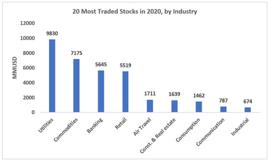
Figure 1.
Twenty most traded shares in 2020, shown by industry. Source: Authors’ own elaboration.
Figure 2 shows the amounts traded in 2020; the twenty shares that make up the IPSA are shown, where the four assets with the highest traded amounts in 2020 correspond to ENELAM (Enel America), SQM-B (Soquimich, Society of Chemistry and Mining of Chile), FALABELLA (Falabella store), and CHILE (Chile Bank).
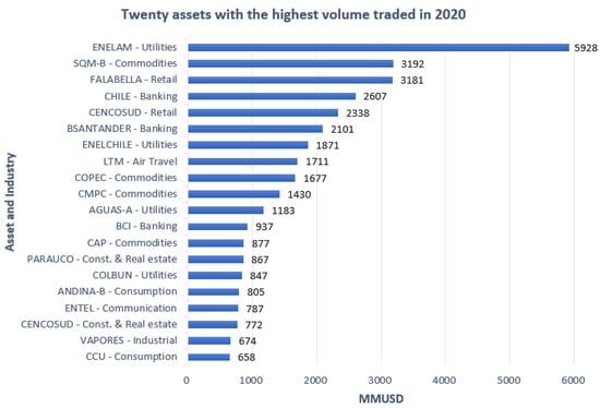
Figure 2.
Amount of 20 most traded shares in 2020, shown by industry. Source: Authors’ own elaboration.
In Figure 3, cumulative returns can be seen between the vertical bars showing the study period delimitations (prior to, during, and after event), where air travel obtained the highest negative profitability, followed by the retail and then the construction and real estate industries, which had a lower proportion. The industries with the fewest crashes in the cumulative return periods were industrial and utilities, followed by the consumption industry.
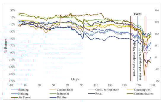
Figure 3.
Cumulative returns by industry for 10 day windows before and after event. Taken from assets belonging to the IPSA. Source: Authors’ own elaboration.
2.2. COVID-19 Pandemic Timetable
In Table 2 we present the important news that affected the movements of assets listed on the Chilean stock market.
Table 2.
COVID-19 pandemic timetable. Source: (CNN Chile 2020).
2.3. Methodology Event Study
To analyze the effect of COVID-19, an event study which included daily returns data from the Santiago Stock Exchange was conducted, specifically to the shares listed in the IPSA (Selective Stock Price Index), where data included assets grouped by industry.
Event study methodology is widely used in finance to identify the effects of circumstances or occurrences on stock markets, assessing the efficiency level by examining the price adjustment of assets according to news reports that could impact the businesses listed. The objective of the present methodology is to assess whether an abnormal efficiency of actions appears as a result of announcements or events (Martín Ugedo 2003).
The stages of the events study are as follows:
1. Event date determination and estimation periods and announcements
The estimation periods used within an event study can vary and are usually between 100 and 300 days for daily profitability studies and between 24 and 60 months for monthly profitability studies. In this case, longer periods improve the accuracy estimation; however, shorter periods avoid mistakes given that parameters are non-stationary (Peterson 1989).
In Figure 4, t = 0 is the announcement period, the event period goes from T1 + 1 to T2, the previous estimation period goes from T0 to T1, and the after-event estimation period goes from T2 + 1 to T3.
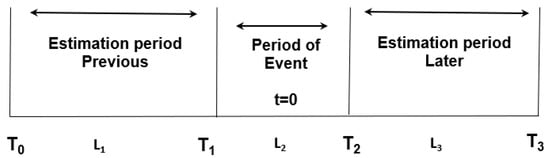
Figure 4.
Event study windows.
The study periods before and after the event had to be established such that they contain enough information to describe what is happening around the return of assets; thus, a range of −10 days to +10 days from T0 (date of initial event) was selected.
2. Estimation of extraordinary profitability
The following equation was used to estimate extraordinary profitability:
where = abnormal return i in time t, = real profitability obtained, = expected profitability, = risk-free rate, = systematic risk, and = expected return market.
The systematic risk (beta) was calculated using the returns of each industrial sector through ordinary least squares estimation. The estimate was made for the 157 days prior to the window prior to the event; then, the systematic risk was calculated for the 10 days after the event.
3. Obtain abnormal returns (AR)
This type of analysis is intended to obtain generalizations, avoiding isolated results of a particular company; therefore, once the abnormal returns (AR) have been estimated, they are cross-aggregated or aggregated by industry.
Calculated for each event date to obtain the residual, this term is mainly used to differentiate the return of share x on day t from the expected return:
where represents the residual difference between , the return of asset i at time t, and , the projected or estimated return.
For every day or month within an event period, residuals are averaged among shares and titles in order to obtain the average residual of the study period, and shares can be grouped by industry or several sectors according to the analysis objectives:
where is the residual average at time t, is the residual shares at time t, and is the sample shares number.
Models Used for Measuring Abnormal Returns
Several models have been developed to review and quantify the returns of normal assets and determine abnormal returns. In this study, we apply three such models (Peterson 1989).
Adjusted Average Return Model—MRPA (method A)
The adjusted average return model assumes that the normal ex ante return for asset i is equivalent to the average daily return of the estimated shares, which can vary between populations. The abnormal return, AR, is the same after deducting the normal return, Rt, from the actual observed return.
where is the abnormal return, is the return of asset i in period t, and is the simple average of asset return in the estimation period.
Adjusted Market Return Model—MRMA (method B)
This is a simpler model that is based on the prior model, where the estimated return of the studied asset is assumed to equal the market return; hence, the model expresses that and , given that alpha is almost consistently a smaller figure and the beta average (systematic risk) from all businesses is as follows:
where is the abnormal return, is the return of asset i in period t, and is the market index return on day t.
Market Model—MM (method C)
This method considers all the market variables and the systematic risk of each asset. This one-factor return model was developed by Sharpe (Sharpe 1963) and is defined in the following equation:
where is the return of asset i at time t, represents returns not explained by the model, is the systematic risk of asset i, is the market return at time t, and is the statistical error.
Profitability for a business is predicted and the event period is acquired through the market model:
This model is known as an index model. Other variants exist for the model, which include different factors (MacKinlay 1997):
where is the abnormal return of stock i on day t and is the expected return obtained using the CAPM.
4. Obtain cumulated abnormal returns (CAR)
At this stage, all abnormal returns are cumulated:
where is the cumulative average residual and is the residual average at time t.
5. Obtain buy-and-hold abnormal returns (BHAR)
In this step, the abnormal return (AR) is calculated based on compound returns (buy-and-hold abnormal returns, or BHAR), where long-term abnormal returns are calculated from short-term returns to obtain the return in the window of the event, following the strategy of buying and holding during said period. Initially, the performance in the event window is estimated for title i using the following expression:
where s is the month of the event, Rit is the return on asset i at time t, and τ is the time horizon after the event.
From BHR (purchase and retention return), the abnormal return obtained (BHAR) is subtracted from the return of the compound asset
Since we have an average cross-sectional sample , the following estimator is used to measure the abnormal behavior of the companies in the sample:
where N is the number of events in the sample, is the weight assigned to company i, and is the time horizon of the calculation after the event.
6. Statistical significance contrasts with extraordinary profitability
A statistical significance review is useful as it can support the study conclusions. When using this method, residual regression outcomes are validated to every period as with the cumulative residual.
The contrasting hypotheses are:
H0 = no evidence of existing abnormal return; and
H1 = evidence of existing abnormal return.
Student’s t-value is calculated using the following equation:
where corresponds to the standard deviation obtained from data in an information-free window related to the event. In this process, the statistical significance must be estimated as follows:
Different shares’ returns are equally and independently distributed as they could include errors, and certain biases can exist when obtaining estimates.
2.4. Analysis of Reaction to New Information in the Market
When news occurs that can affect asset prices in the stock market, these prices can react in a random walk; this was established by Kendall, whose study proposes that a pattern for asset prices that allows prediction of their future prices cannot be established because prices behave randomly in markets that behave efficiently; therefore, the prices of shares become unpredictable (Kendall and Bradford Hill 1953).
Before new information is incorporated into the market, three possible reactions can be visualized:
In Figure 5, the following reactions to an event that affects the stock market can be observed:
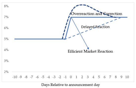
Figure 5.
Event reaction explanation. Source: Own making.
- The incorporation of the new information at time t = 0 and the implementation of a proper correction.
- A positive overreaction to the news, where prices react earlier and slowly correct themselves. It can also be a negative overreaction in the case that the news negatively affects the price of the asset.
- A delayed reaction; the price of the asset does not react at t = 0 before the news release but does react after the news that affects the market.
In points 2 and 3, the market does not react efficiently; therefore, it is inferred that the prices do not behave randomly, as established by Kendall.
3. Results
Parametric and nonparametric tests were used to determine whether these evaluations are robust. These are very specific measures and have worked in countries outside the United States (Campbell et al. 2010). In our case, we assume that the arrival of COVID-19 in Chile generated higher irregular returns, both positive and negative, so the t-statistic will vary significantly from 0.
In Table 3, descriptive return statistics are presented corresponding to a returns diaries sample which was employed in determining the windows for the event study.
Table 3.
Statistical data from the return series used in this study.
Table 3 shows the basic statistics of the data series used where it can be seen among the statigraphists, the kurtosis where it indicates that it is greater than zero, obtaining that the distribution corresponds to a lepticurtic.
In the Table 4 shows a total of a total of 228 daily available returns for the industries within the IPSA were used. The normality tests used for the estimated period data included normality tests from Shapiro–Wilk, Anderson–Darling, Lilliefors, and Jarque–Bera, where the hypotheses were as follows: Hypothesis 0, returns are normally distributed; Hypothesis 1, returns are not normally distributed.
Table 4.
Statistical significance per industry of normality test.
For all industries, the p-value was different than 0 and for some tests was practically zero, thus indicating that the sample for the event study was not normally distributed.
In Figure 6, on the day of the event, the abnormal returns of the industries that make up the IPSA increase following the falls on days −3 and −1, continue to increase until day 3, and then begin to fall from day 4 until day 10, whereas the cumulative abnormal returns continuously decrease until the day of the event, then increase until day 4, and finally continue to decrease.
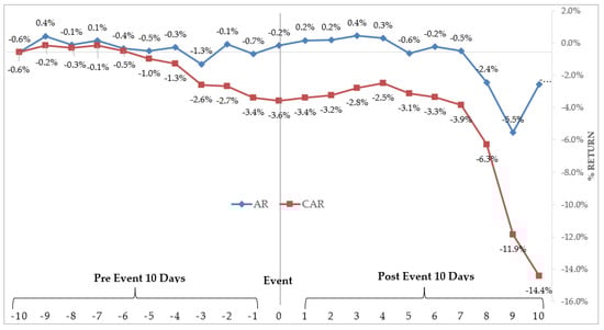
Figure 6.
Abnormal returns and cumulative abnormal returns (MRMA method).
In Figure 7, the abnormal returns are negative on day −10, positive between days −9 and −7 (similar to the obtained cumulative abnormal returns), and then remain negative until the day of the event. However, the abnormal returns from day 1 to day 4 are positive and then become negative from days 5 to 10, whereas the cumulative abnormal returns from day 4 remain negative.
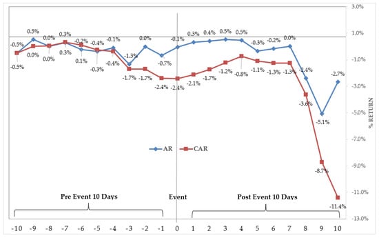
Figure 7.
Abnormal returns and cumulative abnormal returns (MRPA method).
In Figure 8, both the abnormal returns and cumulative abnormal returns are negative until day −4. The abnormal returns remain positive until the day of the event, but then only become positive again on days 6 and 10. However, the cumulative abnormal returns are always negative.
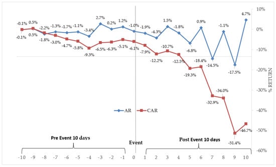
Figure 8.
Abnormal returns and cumulative abnormal returns (MM method).
Since the data sample did not show a normal distribution, it was necessary to use non-parametric tests to evaluate the abnormal returns. Thus, tables showing the results from application of the Wilcoxon signed-rank test are presented.
Given that returns are not normally distributed and have a more leptokurtic form (as generally seen in financial series), it breaks the supposed normality in finance price prediction models, where the tail risk can appear as produced in the real world. The established models with supposed normality cannot model returns movements outside the supposed normality (Sin-Yi 2011). In this case, the asset is shown to be slanted to the left of the curve (negative slant), where a kurtosis excess is given out; the impact is produced by the assignment of assets within a portfolio, especially in crisis periods, as analyzed in the subprime crisis of 2008 (Xiong and Idzorek 2011). Thus, models based on supposed normality, such as asset assessments, can make the mistake to over- or undervalue returns.
Table 5 shows that the Wilcoxon statistics for all days throughout the study window do not have statistical significance; therefore, the null hypothesis cannot be rejected. The population median is thus equal to zero for the abnormal returns obtained using the MRMA method for the industries analyzed in the pre- and post-event windows and on the day of the event, which indicates that the differences in the sample are due to chance.
Table 5.
Wilcoxon signed-rank test, MRMA method.
Table 6 shows that most of the Wilcoxon statistics have no statistical significance both in the pre- and post-event windows and on the day of the event; therefore, the null hypothesis cannot be rejected. The null hypothesis can only be rejected on day 10 post-event. In general, however, on the days studied, the population median is equal to zero among the abnormal returns obtained by the MRPA method of the industries analyzed in the pre- and post-event windows and on the day of the event, indicating that the differences in the sample are due to chance.
Table 6.
Wilcoxon signed-rank test, MRPA method.
Table 7 shows that most of the Wilcoxon statistics have statistical significance, contrary to the data of the other models, and thus the null hypothesis is rejected, except on days −10, −9, −2, 0, 6, and 8. However, in general, on the days studied, the population median is different from zero among the abnormal returns obtained by the MM method for the industries analyzed in the pre- and post-event windows and on the day of the event, which suggests that the differences in the sample are not due to chance.
Table 7.
Wilcoxon signed-rank test, MM method.
In conclusion, the signed-rank test results indicate that there are no significant differences in the abnormal returns data of the industries obtained by the MRMA and MRPA models in the pre-event window, on the day of the event, and in the after-event window; significant differences in the abnormal returns were only obtained by the MM method. This suggests that abnormal returns were affected by the news of the pandemic in the windows before and after the event.
Table 8 shows the results from the paired t-test between the pre- and post-event windows by industry, employed in logarithmic performances from industries listed in the IPSA (Selective Stock Price Index) through the market model method (MM). All industries demonstrated a negative average performance before and after COVID-19′s arrival to Chile, despite previous instances within the banking sector obtained from the abovementioned method. According to the market-adjusted return model (MRPA), the banking sector presented positive average returns in the 10-day pre- and post-event windows; the holding and retail sectors presented positive average returns before the event; and the information technology sector, communication sector, and utilities sector presented positive average returns, all after the event. Regarding the outcomes obtained from the market-adjusted return model (MRPA), the banking sector obtained a positive average return in both windows; however, all other sectors (communication, information technology, air travel, commodities, construction and real estate, holding, and retail) showed negative average returns before and after the event.
Table 8.
Results from the t-test for the pre-event and post-event windows.
All results were obtained by a two-tailed test. The results of all industries have a significance greater than 5% (p > 0.05); however, the null hypothesis cannot yet be rejected.
According to Table 9 and Table 10, the least affected industry before and after the event was the banking sector, and the most affected was air travel. The utilities sector was not affected pre-event according to all the methods, but with the MRPA method, abnormal negative returns during and after the event were noted. To a lesser extent, the consumption, IT, communication, industrial, and retail industries faced a low impact after the virus outbreak in Chile; however, according to the p-values in the post-event window, they became statistically significant. This study aligns with the outcomes from the March 2020 monetary policies report made by the Central Bank of Chile to level IPSA prices, where local financial markets responded strongly in the face of the changing global scenario. As observed in comparable countries, these variables have decayed in ways that have not occurred since the financial crash in 2008. Since the middle of February, the IPSA has descended by up to 32%, registering its worst session in over 30 years (−14.3%, 19 March). The retail, construction, and air travel sectors were the most financially affected (Banco Central de Chile 2020).
Table 9.
CAR results showing the average of the returns before, during, and after the event and their statistical significance.
Table 10.
BHAR results showing the average of the returns before, during, and after the event with their statistical significance.
Figure 9 shows the analysis of accumulated abnormal returns. It is observed that, after the first confirmed case of virus in Chile, the returns were mostly negative. On the other hand, the abnormal returns accumulated after the event showed statistical significance. Here, the financial and utilities sectors were less exposed to a return collapse. This information is useful for the development of investment strategies during a health emergency, considering the systematic risk worldwide.
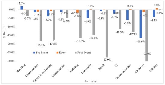
Figure 9.
Cumulative abnormal returns for industries (average of the three methods).
4. Discussion
The following studies were reviewed to justify the application of non-parametric testing for the statistical significance of the event study.
One study reviewed the methodology of event studies with daily returns, evaluating potential problems, such as non-regular data, estimation bias in the regression parameters using a market model, and estimation variance where an increase in the variance indicates excess mean returns within the days after the event (Brown and Warner 1985). For the study of events, it is better to use non-parametric tests than parametric ones, as the latter assume normality of the data, while non-parametric tests do not suppose any type of data distribution. Therefore, to see the robustness of a study, given that the series of financial returns in general are not normally distributed, it is preferable to subject the data to non-parametric tests for studies of events with daily returns (Corrado 1989; Corrado and Zivney 1992). A study with Nasdaq shares revealed an irregularity in developed markets with the application of parametric statistical tests on abnormal returns in an event study. This reinforces that the rank test (non-parametric test) shows the greatest consistency during the event study for the determination of abnormal performance and its statistical significance (Campbell and Wasley 1992).
In our study, non-parametric tests were useful because, after reviewing the data, we found that they were not normally distributed in the period analyzed; therefore, these tests showed that the data are robust from a statistical point of view.
Various studies have been carried out to verify the efficiency of the Chilean securities market. Following the technique of Eugene Fama, an attempt was made to find out if the prices of financial assets of the MILA member countries (Latin American Integrated Market) reflected all the relevant historical information. It was found that, based on the results of the Dickey-Fuller test, the equity markets of Chile, Colombia, Mexico and Peru have weak efficiency (Ramírez et al. 2017). Other researchers have tried to verify the weak efficiency of the five main stock exchanges in Latin America. They used two techniques: first, they tested the normality of the series, where the data was evaluated using basic statistics; then a random walk review was performed under different methods. The finding obtained was that the markets have experienced a change from inefficiency to weak efficiency in the following chronological order: Mexico (2007), Brazil (2008), Colombia (2008), Chile (2011) and Peru (2012) (Duarte and Mascareñas 2014).
This study deals with the efficiency of the market in the period of the arrival of COVID-19 to the Chilean territory, and it has been obtained that the market acted inefficiently, which suggests the non-incorporation of all the market information in the prices of assets. In the previous literature there are factual studies used to explain the effect the pandemic has had on the stock market.
A study carried out with 49 stock indices from different countries using the event study methodology detected strong negative reactions from all the stock indices studied after the virus outbreak, with Asian markets more negatively affected by the entry of the pandemic compared to the United States’ market; the impact was not so significant in both the short and long windows of the study (Pandey and Kumari 2020). Another event study was carried out in the Bangladeshi stock market, obtaining abnormal returns (AR) and cumulative abnormal returns (CAR) through three methods: constant average return, the market return model, and the market model. Here, the first case of COVID-19 caused a negative effect on the stock market, and these results are supported with statistical, parametric, and non-parametric tests (Adnan et al. 2020). Within the Latin American markets, studies have shown a vertiginous fall of the composite indices in the MILA (Integrated Market of Latin America) around March, just when the region faced the arrival of the pandemic. The analysis was carried out with five months of indices’ composite yields within this market, with the IPSA among them (Doria and Nuñez 2020).
Other effects of COVID-19 on the world’s leading stock markets have analyzed where individuals could benefit from a market affected by the pandemic. From this perspective, the markets will react adversely in the short term, so it is possible to invest in companies whose prices have lowered significantly; these low prices will be corrected in the long term. An analysis by industry has been carried out, focusing on the travel, technology, entertainment, and commodities (gold) sectors—areas where big profits can eventually be made (Yan et al. 2020). Another study of the behavior of the stock market indices of Australia, Austria, Belgium, Canada, Denmark, Finland, France, Germany, the United Kingdom, Spain, Ireland, Israel, Italy, the Netherlands, New Zealand, Norway, Portugal, Singapore, Sweden, Switzerland, Japan, and the United States found that the stock exchanges do not always incorporate all the available information; in many cases, they act slowly when evaluating the news. Using a simple statistical analysis, it was shown that the response of the markets to the available information was irrational and ineffective. The COVID-19 outbreak is given as an example of an underestimation of health risk and an unexpectedly slow response during the event; the authors suggest that this phenomenon should be examined in the future from a behavioral perspective, and that it provides an opportunity to search for necessary corrections of asset valuation models for this new world scenario (Vasileiou et al. 2021). A study on the United States’ capital market showed that the market was inefficient during the weeks after the start of the COVID-19 pandemic. This inefficiency meant that agents could maximize their profits from February until the end of March 2020, and they could generate windfall profits by only using historical prices and virus-related data to forecast future equity ETF returns (Navratil et al. 2021). According to research carried out using the event study methodology regarding the efficiency of the markets of emerging economies called BRIC (Brazil, Russia, India, and China), all these markets accumulated negative abnormal returns, with the exception of China. Of the four countries, only China had a better response between the announcement of H1N1 and COVID-19, possibly due to the transformation capacity of its companies in the H1N1 emergency, thus complying with the hypothesis of efficient EMH markets as it reduced anxiety, causing a more effective reaction from the stock markets and providing semi-strong efficiency (Sepúlveda et al. 2021). Furthermore, in a study on the reaction of the stock markets of G20 countries to the COVID-19 outbreak, a negative reaction to the virus outbreak was detected; however, the accumulated abnormal returns gradually turned positive. The conclusion and recommendation regarding the overreaction of the markets is that investors should have long-term investment strategies in the face of outbreaks, buying shares in the short term, with returns negatively affected by the arrival of the pandemic (Singh et al. 2020). Another study involving the Dhaka Stock Exchange of Bangladesh reviewed the hypothesis of randomness in the returns of shares in the face of the pandemic. It was found that the Dhaka Stock Exchange did not show even weak efficiency in the analyzed period (Ahmed 2021). Meanwhile, one study of various indices of various stock markets suggested that the studied markets overreacted with prices (overreaction), and as more information became available, this was corrected (Phan and Narayan 2020). Regarding the S&P500 index in the United States financial market, it was found that this developed market was not always efficient in the face of the COVID-19 outbreak (Evangelos 2020). Another study regarding the effect of health emergencies on stock values in the Asian region considering the SARS outbreak found a short-term window in which China and Vietnam were affected, whereas other countries’ stock markets faced no negative impacts (Nippani and Washer 2004). Additionally, other studies have focused on certain industries, specifically the hospitality industry, which, in theory, faced a greater impact because of sanitary regulations and border closures. A study of this nature was conducted in Taiwan following the SARS virus outbreak and showed an impact on shared returns for the hospitality industry of the country (Chen et al. 2007).
Like other markets, the Chilean stock market has shown great losses with the global health emergency, as can be seen in the results; only the utilities sector was less affected. With this state of the market, as indicated in previous studies, it is useful to apply a long-term investment strategy, since the falling prices of the assets are expected to be corrected in the long term. As in previous studies, the Chilean market is also showing a slow incorporation of information in the price of assets.
5. Conclusions
Financial and general markets come to be unstable and unpredictable during times of pandemic; thus, this work aimed to review COVID-19′s effect within the Chilean stock market. From day one, since the first COVID-19 case in Chile was announced, the majority of firms listed in the IPSA have had negative cumulative abnormal returns according to all applied methods, except the utility sector, and to a lesser extent obtained positive cumulative abnormal returns according to the applied models within the consumption, industrial, IT, and communications sectors.
However, the results were not statistically significant in the post-event window. The IPSA (Selective Stock Price Index) reacted inefficiently to the COVID-19 outbreak, showing weak efficiency against an established event date, that is, the first virus case in Chile. A post-event overreaction can be found within all IPSA-listed companies, highlighting the inefficiency of the Chilean market.
In summary, the findings of this study are the following. Firstly, the announcement of the first confirmed case in Chile led to negative cumulative abnormal returns, except in the industrial, commodities, and communications sectors, but without statistical significance. In the pre-event window, all non-banking industries obtained negative cumulative abnormal returns, also without statistical significance, and in the post-event window, all sectors except the utilities sector obtained negative cumulative abnormal returns, presenting statistical significance; therefore, this suggests the existence of an exaggerated reaction to the first COVID-19 case in Chile, excluding the commodities sector. Secondly, the utilities sector was less affected by the first case of coronavirus in Chile. Thirdly, in the post-event window analysis, non-banking industries obtained negative cumulative abnormal returns of above -10% with statistical significance, except for the utilities sector, which obtained positive cumulative abnormal returns. Fourthly, the study suggests that the market did not collect all the public information available for the first case of COVID-19 in Chile, and in all sectors except the utilities sector, an overreaction was observed after the analyzed event. Finally, when reviewing the event study, the industries that constitute the IPSA reacted slowly to the information of the pandemic, and abnormal returns were obtained by the three methods used that were other than zero, which suggests the existence of market inefficiency in incorporating the information available in the face of the pandemic and the arrival of the first COVID-19 case in the country.
Based on this contingency and the study of the IPSA by industry, it can be suggested to investment analysts that it is possible to adopt a long-term investment strategy, except in the utilities sector, and it is advisable to buy shares and obtain extraordinary profits once the health emergency has been overcome or the abnormal market returns have been corrected. On the other hand, the utilities sector did not present large losses before, during, and after the outbreak of COVID-19; therefore, it becomes a refuge in this market in the formation of investment portfolios, and pension funds can also be considered a refuge for this market.
In future research, it will be useful to carry out a Granger causality study between the variable of new cases of COVID-19 and the stock index in order to find a better valuation model in the face of this new scenario and this type of market, as well as applying an event study that takes into account heteroscedasticity (GARCH Model) and expanding the market to the indices included in the MILA (Latin American Integrated Market), which considers four Latin countries: Chile, Colombia, Mexico, and Peru.
Author Contributions
Conceptualization, J.L.G. and P.A.G.; methodology, P.A.G.; software, P.A.G.; validation, J.L.G. and P.A.G.; formal analysis, J.L.G. and P.A.G.; investigation, J.L.G. and P.A.G.; resources, J.L.G. and P.A.G.; data curation, P.A.G.; writing—original draft preparation, J.L.G. and P.A.G.; writing—review and editing, J.L.G. and P.A.G.; visualization, J.L.G. and P.A.G.; supervision, J.L.G. and P.A.G.; project administration, J.L.G.; funding acquisition, J.L.G. All authors have read and agreed to the published version of the manuscript.
Funding
This research received support from the Family Business Chair of the University de Lleida.
Institutional Review Board Statement
Not applicable.
Informed Consent Statement
Not applicable.
Data Availability Statement
https://es.investing.com/indices/ipsa-historical-data (accessed on 5 February 2021).
Conflicts of Interest
The authors declare no conflict of interest.
References
- Abuzayed, Bana, Elie Bouri, Nedal Al-Fayoumi, and Naji Jalkh. 2021. Systemic risk spillover across global and country stock markets during the COVID-19 pandemic. Economic Analysis and Policy 71: 180–97. [Google Scholar] [CrossRef]
- Adnan, Abu Taleb Mohammad, Mohammad Mahadi Hasan, and Ezaz Ahmed. 2020. Capital Market Reactions to the Arrival of COVID-19: A Developing Market Perspective. The Economic Research Guardian 10: 97–121. [Google Scholar]
- Ahmed, Fakrul. 2021. Assessment of Capital Market Efficiency in COVID-19. European Journal of Business and Management Research 6: 42–6. [Google Scholar] [CrossRef]
- Albulescu, Claudiu Tiberiu. 2021. COVID-19 and the United States financial markets’ volatility. Finance Research Letters 38: 1–5. [Google Scholar] [CrossRef]
- Banco Central de Chile. 2020. Informe de Política Monetaria. Santiago de Chile: Banco Central de Chile. [Google Scholar]
- Binder, John J. 1998. The Event Study Methodology Since 1969. Review of Quantitative Finance and Accounting 11: 111–37. [Google Scholar] [CrossRef]
- Bolsa de Santiago de Chile. 2021. Bolsa de Santiago. October 6. Available online: https://www.bolsadesantiago.com/ (accessed on 10 July 2021).
- Bouri, Elie, Oguzhan Cepni, David Gabauer, and Rangan Gupta. 2020. Return connectedness across asset classes around the COVID-19 outbreak. International Review of Financial Analysis 73: 1–11. [Google Scholar] [CrossRef]
- Bouri, Elie, Riza Demirer, Rangan Gupta, and Jacobus Nel. 2021. COVID-19 Pandemic and Investor Herding in International Stock Markets. Herding in International Stock Risks 9: 168. [Google Scholar] [CrossRef]
- Brown, Stephen J., and Jerold B. Warner. 1985. Using Daily Stock Returns: The Case of Event Studies*. Journal of Financial Economics 14: 3–31. [Google Scholar] [CrossRef]
- Campbell, Cynthia J., Arnold R. Cowan, and Valentina Salotti. 2010. Multi-Country Event Study Methods. Journal of Banking & Finance 34: 3078–90. [Google Scholar]
- Campbell, Cynthia, and Charles Wasley. 1992. Measuring security price performance using daily NASDAQ returns. Journal of Financial Economics 33: 73–92. [Google Scholar] [CrossRef]
- Chen, Ming-Hsiang, SooCheong (Shawn) Jang, and Woo Gon Kim. 2007. The impact of the SARS outbreak on Taiwanese hotel stock performance: An event-study approach. Hospitality Management 26: 200–12. [Google Scholar] [CrossRef]
- CNN Chile. 2020. Cnnchile. May 5. Available online: https://www.cnnchile.com/coronavirus/hitos-claves-covid-19-chile-mundo-cronologia_20200505/ (accessed on 10 July 2021).
- Corrado, Charles J. 1989. A nomparametric test for abnormal securiy-price performance in event studies. Journal of Financial Economics 23: 385–95. [Google Scholar] [CrossRef]
- Corrado, Charles J., and Terry L. Zivney. 1992. The Specification and Power of the Sign Test in Event Study Hypothesis Tests Using Daily Stock. The Journal of Financial and Quantitative Analysis 27: 465–78. [Google Scholar] [CrossRef]
- Doria, Carlos Fernando, and William Niebles Nuñez. 2020. El mercado integrado latinoamericano-MILA-en tiempo de Covid-19. Revista Aglala 11: 17–37. [Google Scholar]
- Duarte, Juan Juan Benjamín, and Juan Manuel Mascareñas. 2014. Comprobación de la eficiencia débil en los principales mercados. Estudios Gerenciales 30: 365–75. [Google Scholar] [CrossRef] [Green Version]
- Evangelos, Vasileiou. 2020. Efficient Markets Hypothesis in the Time of COVID-19. Review of Economic Analysis 13: 45–62. [Google Scholar]
- Fama, Eugene. 1969. Efficient Capital Markets II. The Journal of Finance 46: 1575–617. [Google Scholar] [CrossRef]
- Fama, Eugene. 1965. Efficient Capital Markets: A Review of Theory and Empirical Work. The Journal of Finance 25: 28–30. [Google Scholar] [CrossRef]
- Fama, Eugene F., Lawrence Fisher, Michael C. Jensen, and Richard Roll. 1970. The Adjustment of Stock Prices to New Information. International Economic Review 10: 1–21. [Google Scholar] [CrossRef]
- Fama, Eugene. 1991. The Behavior of Stock-Market Prices. The Journal of Business, 34–105. [Google Scholar] [CrossRef]
- Funakoshi, Minami, and Travis Hartman. 2020. Mad March: How the Stock Market Is Being Hit by COVID-19. March 23, Available online: https://www.weforum.org/agenda/2020/03/stock-market-volatility-coronavirus/ (accessed on 20 May 2021).
- Hassan, Hashibul, and Shahidullah Kayser. 2019. Ramadan effect on stock market return and trade volume: Evidence from Dhaka Stock Exchange (DSE). Cogent Economics & Finance 7: 1605105. [Google Scholar]
- Kendall, M. G., and A. Bradford Hill. 1953. The Analysis of Economic Time-Series-Part I: Prices. Journal of the Royal Statistical Society. Series A (General) 116: 11–34. [Google Scholar] [CrossRef]
- MacKinlay, A. Craig. 1997. Event Studies in Economics and Finance. Journal of Economic Literature 35: 13–39. [Google Scholar]
- Malkiel, Burton G. 2003. The Eficcient Market Hypothesis and Its Critics. Journal of Economic Perspectives 17: 59–82. [Google Scholar] [CrossRef] [Green Version]
- Martín Ugedo, Juan Francisco. 2003. Metodología de los Estudios de Sucesos: Una Revisión. España: Investigaciones Europeas de Dirección y Economía de la Empresa. [Google Scholar]
- Navratil, Robert, Stephen Taylor, and Jan Vecer. 2021. On equity market inefficiency during the COVID-19 pandemic. International Review of Financial Analysis, 1–9. [Google Scholar] [CrossRef]
- Nippani, Srinivas, and Kenneth M. Washer. 2004. SARS: A non-event for affected countries’ stock. Applied Financial Economics 14: 1105–10. [Google Scholar] [CrossRef]
- Pandey, Dharen Kumar, and Vineeta Kumari. 2020. Event study on the reaction of the developed and emerging stock markets to the 2019-nCoV outbreak. International Review of Economics and Finance, 467–83. [Google Scholar] [CrossRef]
- Peterson, Pamela P. 1989. Event Studies: A Review of Issues and Methodology. Quarterly Journal of Business and Economics 28: 36–66. [Google Scholar]
- Phan, Dinh Hoang, and Paresh Kumar Narayan. 2020. Country Responses and the Reaction of the Stock Market to COVID-19. Emerging Markets Finance and Trade 2020 56: 2138–50. [Google Scholar] [CrossRef]
- Ramírez, Laura Bibiana, Aura María Valencia, and Diana Marcela Villalba. 2017. Evaluación de la eficiencia en nivel débil de la información en los mercados de renta variable de los países pertenecientes al MILA 2011–2016: Una estimación a partir del modelo de Tres Factores de Fama y French. Colombia: Facultad de Ciencias Económicas y Sociales–Universidad de la Salle. [Google Scholar]
- Sepúlveda, Jorge, Pablo Tapia, and Boris Pastén. 2021. Analyzing Stock Market Signals for H1N1 and COVID-19: The BRIC Case. Santiago: Munich Personal RePEc Archive. [Google Scholar]
- Shahzad, Syed Jawad, Muhammad Abubakr Naeem, Zhe Peng, and Elie Bouri. 2021. Asymmetric volatility spillover among Chinese sectors during COVID-19. International Review of Financial Analysis 75: 1–9. [Google Scholar] [CrossRef]
- Sharpe, William F. 1963. A Simplified Model for Portfolio Analysis. Management Science 9: 277–93. [Google Scholar] [CrossRef] [Green Version]
- Singh, Bhanwar, Rosy Dhall, Sahil Narang, and Savita Rawat. 2020. The Outbreak of COVID-19 and Stock Market Responses: An Event Study and Panel Data Analysis for G-20 Countries. Global Business Review 1: 1–26. [Google Scholar] [CrossRef]
- Sin-Yi, Cindy Tsai. 2011. The Real World is Not Normal. Chicago: Morningstar Alternative Investments Observer. [Google Scholar]
- Vasileiou, Evangelos, Aristeidis Samitas, Maria Karagiannaki, and Jagadish Dandu. 2021. Health risk and the efficient market hypothesis in the time of COVID-19. International Review of Applied Economics 35: 210–23. [Google Scholar] [CrossRef]
- Xiong, James X., and Thomas M. Idzorek. 2011. The Impact of Skewness and Fat Tails on the Asset Allocation Decision. Financial Analysts Journal 67: 23–35. [Google Scholar] [CrossRef] [Green Version]
- Yan, Heather, Andy Tu, Logan Stuart, and Qingquan Zhang. 2020. Analysis of the Effect of COVID-19 On the Stock Market and Potential Investing Strategies. Illinois: Gies School of Business, University of Illinois Urbana-Champaign. [Google Scholar]
- Yousaf, Imran, Elie Bouri, Shoaib Ali, and Nehme Azoury. 2021. Gold against Asian Stock Markets during the COVID-19 Outbreak. Journal of Risk and Financial Management 14: 186. [Google Scholar] [CrossRef]
Publisher’s Note: MDPI stays neutral with regard to jurisdictional claims in published maps and institutional affiliations. |
© 2021 by the authors. Licensee MDPI, Basel, Switzerland. This article is an open access article distributed under the terms and conditions of the Creative Commons Attribution (CC BY) license (https://creativecommons.org/licenses/by/4.0/).