Empirical Analysis of MSCI China A-Shares

Abstract

In this paper, we introduce the MSCI China A-shares index (MCASI) and analyze MCASI’s properties. From the perspective of index investment, we found that MCASI’s investor sentiments, both overnight sentiment and BW sentiment, provide significant predictability for future MCASI returns, supported by the in-sample and out-of-sample results. From the perspective of sector investment, we show that the sector portfolio of “information transfer, software and information technology services” performs the best among the 10 sector portfolios. In addition, seven approaches of the optimal portfolio in ten sectors are examined, and the results suggest that the classic Markowitz portfolio approach is recommended. Our empirical analysis is helpful for domestic and foreign investors seeking to form investment strategies for MSCI China A-shares.

1. Introduction

To what extent does the MSCI China A-shares index distinguish the other indices in the Chinese stock market? Can it lead to better investments for both domestic and foreign investors? Does the MSCI China A-shares index indicate the characteristics of the Chinese stock market from investor sentiment, liquidity, volatility, sector, and return perspectives? These are the questions we study in this paper. Based on the MSCI index methodology, MSCI China A-shares (Appendix A) now constitute 236 stocks in more than 10 different sectors with constant outperformance, even in the 2015 Chinese stock market crashes. We diagnose MSCI China A-shares in ways ranging from basic returns and volatility to sentiment and liquidity, along with seasonal and sector analysis for trading strategies and investment suggestions. The first question is simply addressed by making comparisons among MSCI China A-shares, the Shanghai composite index (SSEC), and the Shenzhen component index (SZI) for a sample period from January 2010 to December 2018. MSCI China A-shares had positive returns and a positive Sharpe ratio with the smallest maximum drawdown. Both SSEC and SZI had negative returns and Sharpe ratios with bigger maximum drawdowns.

The Chinese capital market has been constantly stoked to open up the financial market to more investing by foreigners and foreign institutions. Foreign institutions invested in the interbank bond market through QFII (quota doubled to USD 300 billion in January 2019) and RQFII systems in the Shanghai and Hong Kong stock connect program in 2002, and the MSCI emerging market index included 200 Chinese stock A-shares on 1 June 2018, and had 236 in 2019. China will continue to make incremental changes to open up its markets, and its efforts will be recognized through greater inclusion in due course. The MSCI China A-shares index will be an important index not only for the Chinese capital market, but also for global investors. The study of Chakrabarti et al. (2005) documented the effect of changes in the MSCI countries indices on the returns and liquidity of the addition and deletion of stocks. The authors of Leuz et al. (2008) found that foreign institutional investors have a strong preference for picking constituents in the MSCI index and Hung and Shiu (2016) found that the trading behaviors of different groups of market participants and ownership changes of firms added to or deleted from the MSCI Taiwan index provide a better understanding of trader behavior around constituent changes and effects on abnormal returns and liquidity. The authors of Chen et al. (2019) further tested the investor awareness hypothesis and illustrated that the positive abnormal returns of additions in MSCI are significantly higher in emerging countries than in developed countries.

The authors of Gao and Chen (2017) explained the significance of Chinese stock A-shares in the MSCI index to understand the domestic investors’ investment behaviors through the comparison of indices’ volatilities, the risk premium effect, and the spillover effect. Instead of the investor awareness hypothesis, effects from additions and deletions, and effects on the currency market, we focus on characterizing the MSCI China A-shares index as an index gathered through returns, sentiments, liquidity, and volatility, and uncover the sector structure of the MSCI China A-shares regarding the performance of sector portfolios. This analysis should help local and global investors to better invest in the Chinese Capital Market.

In this paper, we introduce the MSCI China A-shares index (MCASI) with equal weights on its constituents; then, we calculate MCASI’s returns and other characteristics, including volatility, overnight sentiment, BW sentiment, liquidity measures by price impact Amihud (2002), and the trade-time liquidity of Barardehi et al. (2018). We also directly compare MCASI and other Chinese stock market indices to show the excellent performance of MCASI. In particular, MCASI had a positive average monthly return of 1.12%, and a positive Sharpe ratio whose maximum was 45.08% for the sample period from January 2010 to December 2018. In contrast, both the Shanghai composite index and the Shenzhen component index had negative average monthly returns of −0.05% and −0.31%, respectively, and negative Sharpe ratios of −13.04% and −23.60%, respectively, for the same period. Moreover, the small maximum drawdown of 36.11% was MCASI’s, which indicates that MCASI has lower risk exposure. The Shenzhen component index had the largest maximum drawdown 55.03%, and the Shanghai composite index had a 45.92% maximum drawdown. The results simply answer the first question to confirm the importance of roles of the MSCI China A-shares in the Chinese stock market.

Many studies investigate the relations among market characteristics (Audrino et al. 2019; Baker and Wurgler 2006; Baker et al. 2012; Chowdhury et al. 2018; Liu 2015). To understand the mutual relations among MCASI’s investor sentiment, liquidity, and volatility, our empirical results show that the BW sentiment’s Granger causes the liquidity and the overnight sentiment. We further analyzed whether MCASI’s sentiment, liquidity, and volatility can forecast MCASI’s return. Some studies have concluded that public sentiment can be used to predict stock market movements (Da et al. 2014; Joseph et al. 2011). In Lee et al. (2015), the relations among market volatility, market return, and aggregate equity fund flows are tested. The authors of Ma et al. (2018) examined the interactions among market volatility, liquidity shocks, and stock returns in 41 countries over the period 1990-–2015 and found that liquidity is an important channel through which market volatility affects stock returns in international markets. From in-sample and out-of-sample perspectives, we show that MCASI’s BW sentiment and the differential of MCASI’s overnight sentiment have significant positive predictabilities. These findings can help investors to use the index.

We further examined the properties of sectors in MCASI and the optimal portfolios of these sectors. There are 10 sector portfolios. The manufacturing and the finance sectors have the most stocks. The sector portfolio of "information transfer, software and information technology services" has the largest monthly average return of 2.06%, and the portfolio of mining and quarrying has the lowest monthly average return. We also detected the impact of sector portfolios’ returns on the future MCASI return. Regarding the construction sector and the information transfer sector, software and information technology services have significant and positive effects on their future MCASI returns. Our optimal portfolio results show that the minimum-variance portfolio (MVP), the classic Markowitz portfolio approach, has the highest average monthly returns of 1.9% and the best Sharpe ratio of 0.79. In terms of portfolio risks, MVP with the lowest max drawdown also has an advantage among all optimal portfolios. This sector analysis further helps both domestic and foreign investors to understand different sectors in MSCI China A-shares and conduct their strategies using the aspects of sectors and optimal portfolios.

The article is structured as follows. Section 2 shows our variables and data. We present our empirical results in Section 3 and conclude in Section 4.

2. Variables and Data

The MSCI China A-shares index (MCASI) is constructed with the relevant 236 stocks1 of China A-shares in the MSCI Emerging Market Index published by MSCI in August 2018. We briefly introduce MSCI China A-shares in the appendix. In this section, we evaluate MCASI characteristics, including the return, volatility, investor sentiment, and liquidity. We uniformly allocate an equal weight to each stock when performing calculations of these index features for simplicity.

2.1. MCASI’s Return and Volatility

MCASI’s return is constructed by

$$R{M}_t=\frac{1}{N_t}\sum _{i=1}^{N_t}{r}_{i,t},$$

(1)

where $r_{i,t}$ is the return of stock i for month t and $N_t$ denotes the number of tradable stocks in MCASI for month t.

MCASI’s volatility is defined as the aggregation of the standard deviation of all stocks’ daily returns for a given month,

$$R{V}_t=\frac{1}{N_t}\sum _{i=1}^{N_t}{\sigma }_{i,t},$$

(2)

where ${\sigma }_{i,t}$ is the standard deviation of the daily returns for stock i in month t and $N_t$ is the number of tradable stocks for month t.

Table 1. Codes of MSCI China A-shares in the Chinese Stock Market.

000001	000002	000027	000039	000050	000060	000063	000069
000100	000157	000166	000333	000338	000402	000413	000423
000425	000538	000559	000568	000581	000625	000627	000630
000651	000656	000709	000725	000728	000768	000776	000783
000792	000826	000839	000858	000876	000883	000895	000898
000938	000963	000983	000999	001979	002008	002024	002027
002044	002065	002081	002142	002146	002153	002180	002195
002202	002230	002236	002241	002294	002304	002385	002415
002422	002456	002460	002465	002466	002475	002493	002500
002508	002555	002558	002594	002602	002624	002673	002714
002736	002797	600000	600008	600009	600010	600011	600015
600016	600018	600019	600023	600027	600028	600029	600030
600031	600036	600048	600050	600061	600066	600068	600085
600089	600104	600109	600111	600115	600118	600153	600177
600196	600208	600271	600276	600297	600332	600340	600346
600352	600362	600372	600373	600383	600398	600406	600415
600436	600438	600482	600487	600489	600516	600518	600519
600535	600547	600570	600583	600585	600588	600600	600606
600637	600642	600660	600674	600688	600690	600703	600705
600739	600741	600760	600795	600804	600808	600809	600816
600820	600837	600867	600886	600887	600893	600895	600900
600909	600919	600926	600958	600977	600998	600999	601006
601009	601012	601018	601021	601088	601098	601111	601117
601155	601166	601169	601186	601198	601211	601225	601229
601238	601288	601318	601328	601333	601336	601377	601398
601555	601601	601607	601611	601618	601628	601668	601669
601688	601699	601718	601727	601766	601788	601800	601818
601857	601866	601877	601888	601899	601901	601919	601933
601939	601958	601966	601985	601988	601992	601997	601998
603288	603799	603858	603993

introduces the stock codes of MSCI China A share constituents in the Chinese stock market. There are 236 stocks in total. In August, 2018, MSCI Equity Indexes August 2018 Index Review indicates that MSCI will implement the second step of the partial inclusion of China A-shares in the MSCI China Index as well as relevant composite indexes such as the MSCI Emerging Market Index. Existing China A share constituents will have their weights increased following the increase in the inclusion factor from 2.5% to 5% of their respective FIF-adjusted market capitalization. In addition, ten China A-shares will be added as part of this Index Review at 5% of their FIF-adjusted market capitalization, bringing the total China A-shares included in the MSCI China Index to 236, representing 0.75% of the MSCI Emerging Markets Index.

2.2. MCASI’s Investor Sentiment

There are two sentiment measures of overnight sentiment and BW sentiment to adapt to MCASI. The studies Berkman et al. (2012) and Aboody et al. (2018) suggest that overnight (close-to-open) return can serve as a measure of firm-level investor sentiment. The authors of Berkman et al. (2012) document that individuals tend to place orders outside of normal working hours, and those orders will be executed at the start of the next trading day. Additionally, the study of Li and Li (2021) develops the market-level aggregation of overnight returns treated as firm-specific sentiments. Drawing on Li and Li (2021), we further design a new indicator to capture the whole effect of individual stocks’ investor sentiments measured by overnight returns in MCASI. We focus on two sides of cross-sectional investors’ sentiments, which are the power of optimistic investors and pessimistic investors, respectively2. Specifically, our calculation of the daily MCASI’s overnight sentiment is

$$Sen{t}_{ON,d}=max(0,CT{O}_{optimism,d})+min(0,CT{O}_{pessimism,d}),$$

(3)

where $CT{O}_{optimism,d}$ denotes the average overnight returns of stocks which are the bottom 30% after ranking all stocks by their overnight returns in ascending order on day d, and $CT{O}_{pessimism,d}$ is the average overnight return of the top 30% stocks, N is the numbers of all tradable stocks on day d, and $CT{O}_{i,d}$ represents the overnight return of firm i on day d. Then, we aggregate the daily overnight sentiment to month frequency by averaging them for specific month—specifically, $Sen{t}_{ON,t}=\frac{1}{n}{\sum }_{i=1}^{n}Sen{t}_{ON,t_i}$, where $t_i$ and n are the trading days of month t and the number of all trading days for that month, respectively.

The authors of Baker and Wurgler (2006) use principal component analysis (PCA) to compress six sentiment variables and extract the first principal component as the market sentiment, generally called the BW sentiment, which is widely used in empirical studies. We calculate the BW sentiment according to the procedures of Baker and Wurgler (2006). Due to the availability of corresponding data and the appropriate application of the sentiment index to the Chinese stock market, we selected three individual sentiment proxies: turnover, seasoned equity offerings (SEOs) initial return, and mutual fund premium rate. Turnover is the most direct and the most commonly used as a sentiment variable, and high turnover often means that investors are more active, especially retail investors. In the Chinese stock market, initial public offerings issues (IPOs) have some limitations and a lack of freedom. Additionally, due to the focus on the MSCI China A-shares, it is not appropriate to choose the IPO’s initial return as the sentiment proxy. Prior research indicates that firms that conduct SEOs typically have high equity market value just prior to the SEO, which is called the market-timing theory, which stands for the practice of issuing shares at high prices and repurchasing them at low prices (Asquith and Mullins 1986; Baker and Wurgler 2002; Loughran and Ritter 1995, 1997; Masulis and Korwar 1986). Moreover, Chen et al. (2019) provides empirical evidence that investor sentiment has a positive impact on the SEO probability, where they use the standard BW sentiment of Baker and Wurgler (2006) to measure the market investor sentiment. According to this relation, SEOs reflect some investor sentiment; further, instead of using issues volume of SEOs, we chose the SEO’s initial return as our second proxy in BW sentiment to directly measure the corresponding investor response. The third sentiment proxy is the mutual fund premium rate, and the proxy directly measures investors’ pursuit of mutual funds and their investment enthusiasm. The higher premium rate represents a higher investor sentiment.

We used principal component analysis (PCA) method to compress the above three variables and took the first principal component as the BW investor sentiment3. By fitting the PCA model, the first principal component explains 58.03% of the sample variance, accurately capturing the co-movement of individual sentiment proxies. We used the first principal component to represent our MCASI’s BW sentiment,

$$Sen{t}_{BW,t}=9.43FundC{R}_t+4.42Turnove{r}_t+8.92SE{O}_t,$$

(4)

where $FundC{R}_t$ refers to mutual fund premium rate for month t (the average of the premium rate of all mutual funds in t month), $Turnove{r}_t$ denotes MCASI’s turnover for month t (equal-weight turnover average of all stocks in MCASI), and $SE{O}_t$ represents SEO’s initial return for month t (averaging the SEO initial return of all stocks in MCASI for a given day at first, then aggregating the daily time series to monthly frequency by averaging).

2.3. MCASI’s Liquidity

There are two measures of MCASI’s liquidity: (1) The first liquidity measure is the price impact introduced by Amihud (2002). (2) The second one is the trade-time liquidity introduced by Barardehi et al. (2018). The first liquidity measure is an illiquidity measure (the larger the value, the worse the liquidity). We calculate the Amihud liquidity for firm i on day d as:

$$P{I}_{i,d}=\frac{|r_{i,d}|}{V_{i,d}},$$

(5)

where $r_{i,d}$ is the return of firm i on day d, and $V_{i,d}$ is the CNY volume of firm i on day d. For constructing MCASI’s liquidity, we first take equal-weight average for liquidity of all stocks in MCASI for a given day, then aggregate the daily time series to monthly frequency by equally averaging.

The second liquidity measure is the trade-time liquidity. We developed our trade-time liquidity indicator based on the method of Barardehi et al. (2018), where the trade-time liquidity measure reflects the per-dollar price impacts of fixed-dollar volumes. Specifically, our firm’s trade-time liquidity $TT{L}_t$ is defined, for day t, by

$$n_t=argmi{n}_{n^{*}}\{\sum _{n=1}^{n^{*}}{P}_{t-n}{Q}_{t-n}|\sum _{n=1}^{n^{*}}{P}_{t-n}{Q}_{t-n}>\lambda M{V}_t\},$$

(6)

$$TT{L}_t=|\frac{P_t-P_{t-n_t}}{P_{t-n_t}}|\frac{1}{{\sum }_{n=1}^{n_t}{P}_{t-n}{Q}_{t-n}},$$

(7)

where $P_t$, $Q_t$ and $M{V}_t$ are the price, the volume and the market value for a stock on day t respectively, and $\lambda$ is an adjustable parameter (we set it to be 0.02). The liquidity measure is different from the one in Barardehi et al. (2018). We used a rolling operation to determine the latest liquidity indicator. Specifically, for the calculation of $n_t$, we used the fixed end time to find the historical start time, but they used the fixed start time to find future end time because their time periods are not crossed. For any moment, our procedure allows us to use the historical information available to calculate the latest liquidity right now. However, the procedure of Barardehi et al. (2018) needs to wait for the information of future trade flow to finish the calculation of the latest $n_t$. However, $TTL$ calculated by their procedure does not include duplicate price or volume information, which let every $TTL$ node have access to the unique information. Of course, the latest daily trade-time liquidity in our definition does not seriously affect the aggregation calculations to form the lower frequency liquidity, but it is always better to obtain the new information.

We calculated the trade-time liquidity $TT{L}_t$ for each individual stock every day, and average them in cross section to obtain a daily aggregated liquidity time series, then average the daily time series to monthly frequency. Our trade-time liquidity TTL${}_t$ defined by similar method of Barardehi et al. (2018) has an innovated modification and improvement to use the latest information and aggregate daily information for individual stocks.

The calculation of trade-time liquidity can be adjusted according to investors’ long-term and short-term liquidity needs by changing the $\lambda$ in Equation (4). Compared with price impact, trade-time liquidity has higher information content and is more flexible and changeable to utilize without losing liquidity information. Considering the numerical issue that these values are too close to zero for these two liquidity measures, we take logarithm on them.

2.4. Data Descriptive

We collect data from the CSMAR database of the Chinese stock market. The sample period is chosen from January 2010 to December 2018. Individual stock data only relates to MSCI China A-shares, totaling 236 stocks. We first present basic data statistical description. Then we provide the correlation analysis and the seasonality analysis for our variables in the sample period.

Table 2. Description Statistics.

Panel A. Variables’s Statistics
Variables	No. of Obs.	Mean	Min	Max	Std	Skew	Kurtosis
FundCR	108	0.0004	−0.1732	0.3112	0.0622	1.2855	6.1792
Turnover	108	0.1950	0.0867	0.6621	0.1140	2.4201	6.1693
SEO	108	0.0000	−0.0141	0.0166	0.0051	0.3524	1.1779
$Sen{t}_{ON}$	108	−0.0015	−0.0117	0.0070	0.0031	−0.4345	2.2259
$Sen{t}_{BW}$	108	0.0000	−0.3067	0.3247	0.0967	0.4534	1.8404
PI	108	−23.66	−25.17	−22.40	0.6234	−0.1164	−0.7739
TTL	108	−24.46	−25.48	−23.32	0.5609	−0.1028	−1.1286
RV	108	0.0230	0.0131	0.0622	0.0082	2.3147	6.9304
RM	108	0.0112	−0.2327	0.1942	0.0709	0.0010	1.2116
Panel B. MCASI, SSEC and SZI
Indexes		MCASI		SSEC		SZI
Mean		0.0112		−0.0005		−0.0031
Std		0.0709		0.0644		0.0744
Sharpe Ratio		0.4508		−0.1304		−0.2360
Maximum		0.3611		0.4592		0.5503
Drawdown

gives the basic statistical description of our variables in Panel A, which are all monthly frequency (total 108 monthly observations). The mean of MCASI’s overnight sentiment ($Sen{t}_{ON}$) is negative (−0.15%) and the skewness is −0.4345, indicating that investor sentiment on MCASI tends to be pessimistic during the sample period. Figure 1 presents time-series charts of our variables for the MSCI China A-shares during the sample period. It is worth noting that there are distinct step shapes on charts of two liquidity indicators, price impact and trade-time liquidity, which means that after the financial crash in 2015, MCASI’s liquidity has become better.

Panel B of Table 2 compares performances of MCASI, SSEC and SZI in our sample period, where SSEC and SZI stand for Shanghai Composite Index and Shenzhen Component Index respectively. Compared with SSEC and SZI, MCASI has a positive average monthly return of 1.12%, a positive and maximum Sharpe ratio of 0.4508. Both SSEC and SZI have negative average monthly returns −0.05% and −0.31% respectively, and negative Sharpe ratios −13.04% and −23.60% respectively. Moreover, the smallest maximum drawdown is existing in MCASI which indicates that MCASI has lower risk exposure4. The Shenzhen Component Index exposes the largest maximum drawdown 55.03%. Figure 2 shows cumulative returns of MCASI, SSEC and SZI, where MCASI has a huge advantage over the two common market indexes in the Chinese stock market. The stable earning of MCASI constructed by MSCI China A-shares consistently performs best in the 2015 Chinese stock market crash. Cumulative returns of SSEC and SZI consistently perform negative returns since 2010 with a little hump from the earlier positive gain in 2015.

Table 3. Correlation analysis of variables of MCASI.

Variables	FundCR	Turnover	SEO	${\mathit{Sent}}_{\mathit{BW}}$	${\mathit{Sent}}_{\mathit{ON}}$	PI	TTL	RV	RM
FundCR	1.000 ***	0.256 ***	0.656 ***	0.907 ***	0.400 ***	−0.341 ***	−0.313 ***	0.015 ***	0.792 ***
Turnover	0.256 ***	1.000 ***	0.097	0.425 ***	0.175 *	−0.561 ***	−0.327 ***	0.742 ***	0.189 *
SEO	0.656 ***	0.097	1.000 ***	0.859 ***	0.571 ***	−0.189 *	−0.145	−0.200 **	0.888 ***
$Sen{t}_{BW}$	0.907 ***	0.425 ***	0.859 ***	1.000 ***	0.533 ***	−0.408 ***	−0.314 ***	0.090	0.897 ***
$Sen{t}_{ON}$	0.400 ***	0.175 *	0.571 ***	0.533 ***	1.000 ***	−0.354 ***	−0.339 ***	−0.281 ***	0.667 ***
PI	−0.341 ***	−0.561 ***	−0.189 *	−0.408 ***	−0.354 ***	1.000 ***	0.944 ***	−0.167 *	−0.306 ***
TTL	−0.313 ***	−0.327 ***	−0.145	−0.314 ***	−0.339 ***	0.944 ***	1.000 ***	0.060	−0.256 ***
RV	0.015	0.742 ***	−0.200 **	0.09	−0.281 ***	−0.167 *	0.060	1.000 ***	−0.216 **
RM	0.792 ***	0.189 *	0.888 ***	0.897 ***	0.667 ***	−0.306 ***	−0.256 ***	−0.216 **	1.000 ***

The statistical significance marks are in parentheses below the corresponding coefficients. *, **, and *** indicate (2-sided) statistical significance at the 10%, 5%, and 1% levels, respectively. The sample period extends from January 2010 to December 2018.

presents the Pearson correlations among these variables. For MCASI’s BW sentiment, there is a significant and positive correlation (53.3%) with the overnight sentiment, which represents these two sentiment measures capture some common sentiment information. MCASI’s BW sentiment has a significant and positive correlation with MCASI’s return, reaching 89.7%. MCASI’s overnight sentiment has significant correlation with all other variables. In addition, the correlation between price impact and trade-time liquidity of MCASI is very high, reaching 94.4%.

Table 2 provides descriptive statistics of our variables. All variables are described in the Variables Definition section. FundCR refers to the mutual fund premium rate. Turnover denotes MCASI’s turnover which is an equal-weight turnover average of all stocks in MCASI. SEO represents the SEO’s initial return. $Sen{t}_{ON}$ and $Sen{t}_{BW}$ are MCASI’s overnight sentiment and BW sentiment, respectively. PI and TTL are MCASI’s liquidity measures of Amihud liquidity and trade-time liquidity, respectively. RV refers to MCASI’s volatility which is the aggregation of the standard deviation of daily returns of all stocks in MCASI for a given month. SSEC and SZI stand for the Shanghai Composite Index and Shenzhen Component Index, respectively. The sample period extends from January 2010 to December 2018.

Table 3 presents the correlation analysis of our variables. All variables are as described in the text. FundCR refers to mutual fund premium rate. Turnover denotes MCASI’s turnover which is equal-weight turnover average of all stocks in MCASI. SEO represents SEO’s initial return. $Sen{t}_{ON}$ and $Sen{t}_{BW}$ are MCASI’s overnight sentiment and BW sentiment, respectively. PI and TTL are MCASI’s liquidity measures of Amihud liquidity and trade-time liquidity, respectively. RV refers to MCASI’s volatility which is the aggregation of the standard deviation of daily returns of all stocks in MCASI for a given month.

Table 4. Seasonality analysis of variables of MCASI.

	FundCR (%)	Turnover (%)	SEO (%)	${\mathit{Sent}}_{\mathit{BW}}$ (%)	${\mathit{Sent}}_{\mathit{ON}}$ (%)	PI	TTL	RV (%)	RM (%)
Month
1	−3.30	19.60	−0.05	−4.47	−0.24	−23.56	−24.33	2.63	−1.57
2	0.95	14.73	0.37	3.22	−0.10	−23.69	−24.42	2.35	3.67
3	0.74	22.38	0.15	1.85	−0.06	−23.79	−24.57	2.14	2.12
4	−1.31	21.12	0.09	−0.76	−0.08	−23.79	−24.58	2.18	1.35
5	−0.11	19.09	0.01	−1.25	−0.19	−23.64	−24.47	2.23	0.98
6	−3.10	19.25	−0.14	−5.51	−0.24	−23.57	−24.39	2.33	−2.69
7	0.33	21.94	0.15	1.43	−0.29	−23.59	−24.39	2.51	1.69
8	−0.61	20.96	0.11	−0.02	−0.25	−23.61	−24.46	2.36	−0.09
9	2.00	16.96	0.08	0.86	−0.11	−23.58	−24.46	2.14	0.73
10	1.79	15.76	0.19	1.89	−0.01	−23.63	−24.47	2.31	3.36
11	−0.11	21.56	0.02	−0.55	−0.05	−23.76	−24.56	2.22	1.52
12	3.23	20.61	0.13	3.29	−0.13	−23.67	−24.44	2.23	2.34
Quarter
1	−0.54	18.90	0.16	−0.20	−0.13	−23.68	−24.44	2.37	1.41
2	−1.51	19.82	−0.01	−2.50	−0.17	−23.66	−24.48	2.25	−0.12
3	0.58	19.95	0.11	0.76	−0.22	−23.59	−24.44	2.34	0.78
4	1.64	19.31	0.12	1.54	−0.06	−23.69	−24.49	2.25	2.41
Year
2010	−4.71	21.42	0.14	−2.88	−0.18	−23.41	−24.09	2.48	1.49
2011	−3.41	14.51	−0.05	−5.61	−0.24	−23.13	−23.95	2.09	−1.99
2012	−0.15	12.63	0.17	−0.63	−0.22	−22.84	−23.79	2.00	1.62
2013	0.12	16.74	0.11	−0.27	−0.11	−23.21	−24.03	2.28	1.15
2014	4.15	21.76	0.25	5.72	0.01	−23.60	−24.40	2.13	4.73
2015	4.11	42.68	0.25	9.97	−0.05	−24.50	−24.96	3.78	3.59
2016	−0.12	17.61	−0.05	−2.27	−0.18	−24.05	−24.94	2.14	−0.30
2017	0.39	15.36	0.09	−0.67	−0.15	−24.34	−25.22	1.65	1.77
2018	−0.02	12.74	−0.06	−3.36	−0.20	−23.82	−24.77	2.18	−2.00

illustrates the seasonality analysis of variables with respect to the aggregate averages over a month, a quarter and a year. In terms of monthly aggregation, the BW sentiment has the lowest average of −5.51% in June and the highest average of 3.29% in December. MCASI’s return has the lowest average of −2.69% in June and the highest average of 3.67% in February, partly due to the high optimism of investor sentiment during the Chinese New Year. In terms of quarterly aggregation, the data for both the BW sentiment and overnight sentiment of MCASI demonstrate that investors are relatively optimistic in the fourth quarter. The data for MCASI’s price impact and trade-time liquidity show that MCASI’s liquidity is also the best in the fourth quarter. In terms of annual aggregation, MCASI’s sentiment is the highest in 2014 and 2015 both for the BW and overnight sentiments, and MCASI’s return also has the highest average in these two years. MCASI’s return is the lowest in 2018, reaching −2.00%. Sent${}_{BW}$ and Sent${}_{ON}$ are the lowest in 2011, at −5.61% and −0.24%, respectively, where MCASI’s return also drops into the near lowest −1.99%. Two liquidity indicators generally show a certain trend; that is, MCASI’s liquidity has become better in recent years.

Table 4 presents seasonal analysis of our variables, which are grouped and averaged for the months, quarters, and years. All variables are as described in the text. FundCR refers to mutual fund premium rate. Turnover denotes MCASI’s turnover which is equal-weight turnover average of all stocks in MCASI. SEO represents SEO’s initial return. $Sen{t}_{ON}$ and $Sen{t}_{BW}$ are MCASI’s overnight sentiment and BW sentiment, respectively. PI and TTL are MCASI’s liquidity measures of Amihud liquidity and trade-time liquidity, respectively. RV refers to MCASI’s volatility which is the aggregation of the standard deviation of daily returns of all stocks in MCASI for a given month. The sample period extends from January 2010 to December 2018.

3. Empirical Results

3.1. Relations among MCASI’s Sentiment, Liquidity, and Volatility

We discuss the relationship among MCASI’s sentiment, liquidity and volatility by adopting the vector autoregression (VAR) model. First-order differential processing is applied in MCASI’s turnover and two liquidity measures to make them stationary. We perform the Dickey–Fuller tests on all variables, and

Table 5. Dickey–Fuller tests of variables.

Variables	T-Statistics
$Sen{t}_{ON}$	−7.26
$Sen{t}_{BW}$	−2.97
FundCR	−8.30
SEO	−9.37
$\mathsf{\Delta }Turnover$	−11.92
$\mathsf{\Delta }PI$	−5.54
$\mathsf{\Delta }TTL$	−6.77
RV	−3.68

shows results that manifest all tests that reject a unit root. We determined the lag numbers of the VAR model by using the Bayesian Information Criterions (BICs), and the BIC is smallest when $L=1$ for the sample.

Table 6. Relations among MCASI’s sentiment, liquidity and volatility.

	Liquidity = $\mathsf{\Delta }\mathit{TTL}$		Liquidity = $\mathsf{\Delta }\mathit{PI}$
	F-Statistics	p-Value	F-Statistics	p-Value
Eqn: $Sen{t}_{BW}$
$Sen{t}_{ON}$	0.149	0.700	0.334	0.564
$Sen{t}_{BW}$	2.928	0.088 *	4.542	0.034 **
Liquidity	0.111	0.739	0.565	0.453
RV	2.794	0.095 *	1.678	0.196
Eqn: $Sen{t}_{ON}$
$Sen{t}_{ON}$	0.264	0.608	0.812	0.368
$Sen{t}_{BW}$	8.893	0.003 ***	14.82	0.000 ***
Liquidity	0.047	0.829	3.132	0.078 *
RV	4.674	0.031 **	8.225	0.004 ***
Eqn: Liquidity
$Sen{t}_{ON}$	5.967	0.015 **	1.065	0.303
$Sen{t}_{BW}$	7.715	0.006 ***	8.240	0.004 ***
Liquidity	4.720	0.030 **	6.114	0.014 **
RV	0.654	0.419	3.603	0.058 *
Eqn: RV
$Sen{t}_{ON}$	21.93	0.000 ***	19.93	0.000 ***
$Sen{t}_{BW}$	0.008	0.930	0.236	0.628
Liquidity	1.303	0.254	0.006	0.940
RV	164.6	0.000 ***	169.7	0.000 ***

All variables are described in the text. *, **, and *** indicate (2-sided) statistical significance at the 10%, 5%, and 1% levels, respectively. The sample period extends from January 2010 to December 2018.

shows the estimates of VAR(1) with corresponding variables. The F-statistics and corresponding P-value test the null hypothesis that the coefficients associated with the row variables are jointly 0 in the VAR equation denoted at the top of the block. In the second and third row blocks, MCASI’s liquidity is measured by trade-time liquidity. In the last two row blocks, MCASI’s liquidity is measured by price impact.

Table 5 presents the results of Dickey–Fuller tests for the corresponding varia described inbles. All variables are the text. FundCR refers to mutual fund premium rate. Turnover denotes MCASI’s turnover which is equal-weight turnover average of all stocks in MCASI. SEO represents SEO’s initial return. $Sen{t}_{ON}$ and $Sen{t}_{BW}$ are MCASI’s overnight sentiment and BW sentiment, respectively. PI and TTL are MCASI’s liquidity measures of Amihud liquidity and trade-time liquidity, respectively. RV refers to MCASI’s volatility which is the aggregation of the standard deviation of daily returns of all stocks in MCASI for a given month. We transform MCASI’s turnover of $Turnover$ and liquidity measures of $TTL$ and $PI$ by differential processing to make them stationary in order to apply VAR, represented by $\mathsf{\Delta }Turnover$, $\mathsf{\Delta }TTL$ and $\mathsf{\Delta }PI$, respectively. The sample period extends from January 2010 to December 2018.

Table 6 shows that MCASI’s BW sentiment, liquidity and volatility are autocorrelated by the VAR model, regardless of whether MCASI’s liquidity measure is trade-time liquidity or price impact. There is evidence to show that MCASI’s BW sentiment Granger causes MCASI’s overnight sentiment, specifically, $F=8.893$ and $P=0.003$ for MCASI’s trade-time liquidity and $F=14.82$ and $P<0.001$ for MCASI’s price impact. MCASI’s volatility Granger also causes the overnight sentiment. The BW sentiment Granger causes both the trade-time liquidity and the price impact. In addition, the overnight sentiment Granger causes the trade-time liquidity with the evidence $P=0.015$, and MCASI’s volatility Granger causes the price impact with the slightly weak evidence $P=0.058$. For MCASI’s volatility, there is no evidence to show that MCASI’s BW sentiment and liquidity are Granger causes, but MCASI’s overnight sentiment is a Granger cause with good statistical significance ($p<0.001$).

Overall, MCASI’s BW sentiment Granger causes the overnight sentiment and liquidity of MCASI. MCASI’s overnight sentiment and MCASI’s volatility are the Granger cause for each other.

3.2. Forecasting MCASI’s Return with MCASI’s Sentiment, Liquidity, and Volatility

It is important to effectively forecast MCASI’s returns for investors. In this section, we investigate whether MCASI’s sentiments, liquidity, and volatility have predictive power with regard to MCASI’s return. We use the first-order differential form of MCASI’s overnight sentiment to conduct the following investigation since MCASI’s overnight sentiment does not have a predictive effect on MCASI’s return but its differential has. There is a certain long-term trend on MCASI’s overnight sentiment, and the differential of MCASI’s overnight sentiment captures the changes of the recent investor sentiment about MCASI, so it is more sensitive and effective for predicting MCASI’s return. Denote $\mathsf{\Delta }Sen{t}_{ON}$ as the differential (or the change) of MCASI’s overnight sentiment in

Table 7. Forecasting MCASI’s return.

Panel A. In-Sample Estimates
Variables	M1	M2	M3	M4	M5	M6	M7	M8	M9
Intercept	0.011	0.011	0.011	0.011	0.030	0.011	0.034	0.011	0.025
$\mathsf{\Delta }Sen{t}_{ON}$	4.812 **	—	—	—	—	5.563 **	5.008 **	4.867 **	4.537 *
$Sen{t}_{BW}$	—	0.130 *	—	—	—	0.156 *	0.194 **	0.098	0.116
$\mathsf{\Delta }PI$	—	—	−0.014	—	—	0.053 *	0.066 *	—	—
$\mathsf{\Delta }TTL$	—	—	—	-0.033	—	—	—	0.023	0.030
RV	—	—	—	—	−0.818	—	−1.024	—	−0.629
Panel B. Out-of-Sample Results
Metrics	M1	M2	M3	M4	M5	M6	M7	M8	M9
$R_{oos}^2$	6.796% **	5.371% ***	−1.169%	3.255% ***	−3.468%	0.298% **	−2.583% *	1.467% **	−3.578% *
MSFE_Adj	1.890	2.421	0.072	2.384	0.055	1.672	1.408	1.710	1.292

The statistical significance marks are in parentheses below the corresponding coefficients. *, **, and *** indicate (2-sided) statistical significance at the 10%, 5%, and 1% levels, respectively. The sample period extends from January 2010 to December 2018.

.

Table 6 presents estimates of VAR(1) with corresponding variables. $Sen{t}_{ON}$ and $Sen{t}_{BW}$ are MCASI’s overnight sentiment and BW sentiment respectively. PI and TTL are MCASI’s liquidity measures of Amihud liquidity and trade-time liquidity, respectively. RV refers to MCASI’s volatility which is the aggregation of the standard deviation of daily returns of all stocks in MCASI for a given month. We transform MCASI’s liquidity measures of $TTL$ and $PI$ by differential processing to make them stationary in order to apply VAR, represented by $\mathsf{\Delta }TTL$ and $\mathsf{\Delta }PI$, respectively. The F-statistics and corresponding p-value test the null hypothesis that the coefficients associated with the row variable are jointly 0 in the VAR equation denoted in the top of block. In the 2nd and 3rd columns, MCASI’s liquidity is measured by trade-time liquidity. In the last 2 columns, MCASI’s liquidity is measured by price impact.

Panel A of Table 7 presents the regression results of forecasting MCASI’s return. For univariate regression models 1–5, MCASI’s BW sentiment and the differential of MCASI’s overnight sentiment have significantly positive predictive effects on MCASI’s return; however, MCASI’s trade-time liquidity and price impact have no predictive effect on MCASI’s return. In multivariate regression models 6–9, the differential of MCASI’s overnight sentiment keeps the significantly positive predictability on MCASI’s return for all four models; MCASI’s BW sentiment and price impact have the significant and positive predictability on MCASI’s return for models 6 and 7, but BW sentiment and trade-time liquidity do not have the significant predictability on MCASI’s return for models 8 and 9. MCASI’s volatility does not show any predictability on MCASI’s return in all models. The differential of MCASI’s overnight sentiment has significantly positive predictability on MCASI’s return in both univariate and multivariate regressions, and MCASI’s BW sentiment has significantly positive predictability on MCASI’s return in univariate and first two partial multivariate regressions. MCASI’s liquidity measures and volatility have no predictive effect on MCASI’s return in univariate and multivariate regressions.

Table 7 introduces estimates of the regressions of predicting MCASI’s return by using MCASI’s sentiment, liquidity and volatility.

In order to further check the out-of-sample performance of these forecasting models, we use the recursive estimation window method to generate forecasts. For each forecast at month t, we used all observations available before month t to estimate models’ coefficients for each model and generate the corresponding forecast. The initial sample for estimating the first forecast is half of the total samples, and all out-of-sample forecasts are from January 2015 to December 2018. We evaluate forecasts’ performances by the out-of-sample r-squared defined by the percent reduction in MSPE of the given model relative to the benchmark model of the historical mean, given by

$$R_{oos}^2=1-\frac{{\sum }_{t=M+1}^T({\widehat{r}}_t-r_t)}{{\sum }_{t=M+1}^T({\overline{r}}_t-r_t)},$$

(8)

where ${\widehat{r}}_t$ is the forecast of the corresponding model at month t, $r_t$ is the realized return, and ${\overline{r}}_t$ is the historical mean. The statistical significance of $R_{oos}^2$ is measured by the adjusted MSFE statistic of Clark and West (2007). A positive and significant $R_{oos}^2$ indicates that the model of interest performs better than the benchmark model.

Panel B of Table 7 presents the out-of-sample results. The univariate model by the changes of MCASI’s overnight sentiment has the highest out-of-sample r-squared of 6.796%. The BW sentiment and the trade-time liquidity also show significant and powerful predictability, which indicates that these two indicators have a more significant impact on MCASI’s return after 2015. The corresponding multivariate models show less predictability.

Overall, the changes of MCASI’s overnight sentiment and the MCASI’s BW sentiment has a significant and positive impact on forecasting MCASI’s return.

3.3. Sector Analysis of MSCI China A-Shares

In order to better understand the MSCI of China A-shares, we further decomposed the related 236 stocks into 10 sectors and examined the performance of each sector in the same sample period. Moreover, we analyzed the predictability of sector returns on MCASI’s return and present a re-portfolio analysis for these 10 sectors with different allocation methods.

3.3.1. Sector Portfolios

In this section, we mainly classify and analyze the MSCI China A-share constituents to distinguish the performances of different industries and analyze whether there is a sector portfolio that performs better than others.

We divided the 236 stocks of MSCI China A-shares into 10 categories by their industry properties, forming 10 sector portfolios. The specific sector codes and names are in Panel A of

Table 8. Sector portfolios of MSCI China A-shares.

Panel A: Sector Code Tag
B	Mining and Quarrying
C	Manufacturing
D	Utilities
E	Construction
F	Wholesale and Retail Trades
G	Transportation, Storage and Postal Services
I	Information Transfer, Software and Information Technology Services
J	Finance
K	Real Estate
O	Others
Panel B: Basic Statistics of Sector Portfolios
	B	C	D	E	F	G	I	J	K	O
Stocks	12	97	12	10	8	11	14	49	13	10
Number
Observations	108	108	108	108	108	108	108	108	108	108
Mean	0.04	1.28	0.64	0.96	0.72	0.59	2.06	1.03	1.21	1.77
(%)
Minimum	−20.99	−23.50	−26.45	−25.88	−18.15	−26.23	−25.33	−22.82	−24.02	−25.87
(%)
Maximum	22.79	15.69	35.70	57.08	22.92	47.78	29.81	39.40	30.27	32.02
(%)
Standard	7.79	7.00	7.46	10.42	7.24	9.19	10.17	9.61	9.50	9.20
Deviation (%)
Skewness	0.26	−0.27	0.60	1.91	0.12	1.42	0.41	1.17	0.56	0.40
Kurtosis	0.46	0.83	5.59	8.55	0.53	6.58	0.77	3.36	1.19	1.31
Annualized	−2.71	22.61	5.35	7.34	7.14	2.57	48.47	10.05	14.38	36.80
Return (%)
Sharpe	−0.07	0.54	0.20	0.25	0.25	0.15	0.64	0.30	0.37	0.59
Ratio
Maximum	−54.93	−33.68	−49.77	−56.22	−39.93	−53.43	−48.93	−41.64	−35.73	−36.71
Drawdown (%)

, where the sector O includes all stocks that do not belong to other nine sectors. Each sector portfolio is constructed by all stocks of this sector with equal weight. For a given month t, the return of the sector portfolio k is $SecRe{t}_{k,t}=\frac{1}{n_k}{\sum }_{i=1}^{n_k}{r}_{k,i,t},$ where $r_{k,i,t}$ denotes the return of stock i in the sector k in month t, and $n_k$ is the number of all stocks in sector k. The cumulative return of the sector portfolio k is calculated as ${\prod }_{j=1}^T(1+SecRe{t}_{k,j})-1$.

Table 8 shows sector information of MSCI China A-shares. Panel A shows that sector code tags of MSCI China A-shares. Panel B show basic data statistics of corresponding sector portfolios. The sample period extends from January 2010 to December 2018.

Panel B of Table 8 gives basic statistics for these sector portfolios. These results show that the manufacturing sector (Code: C) and the finance sector (Code: J) have the most stocks, with 94 and 49, respectively. For the average of portfolio returns (monthly), the sector portfolio of the information transfer, software and information technology services (Code: I), with 14 stocks, has the largest monthly average return of 2.06%, and the sector portfolio of the mining and quarrying (Code: B) has the lowest monthly average return. The minimum monthly returns of these sector portfolios are concentrated around −20% in the interval range (−26.23%, −18.15%). The maximum monthly returns of the sector portfolios of the construction (Code: E) and the transportation, storage and postal services (Code: G) are outstanding in all portfolios, reaching 57.08% and 47.78%, respectively. Sector portfolio I and sector portfolio O have the best annualized returns of 48.47% and 36.80%, respectively, and the annualized return of the sector portfolio B is the only negative value of −2.71% in all sector portfolios. For the performance of the Sharpe ratio, sector portfolios I, O, and C have the highest values of 0.64, 0.59, and 0.54, respectively; the sector portfolio of mining and quarrying (Code: B) has the lowest Sharpe ratio, −0.07. The standard deviation of the returns of the sector portfolios indicates that the portfolio of the manufacturing (C) has lower risk exposure; sector portfolios E, I, J and K (construction sector, IT sector, finance sector and Real estate sector) have the highest risk exposure. In order to further measure the risk attribution of the portfolios, we also calculated the maximum drawdown of their net values, which can be used to measure the maximum loss of the portfolio net value during the investment period. The results of the maximum drawdown show that the portfolio of the manufacturing (C) has the lowest historical maximum drawdown (the lowest risk exposure) in all sector portfolios, and the portfolio of constructions (E) has the maximum risk exposure. Both mining and quarrying (B), transportation (G), utilities (D) and information technology (I) are sectors with relatively higher maximum drawdown.

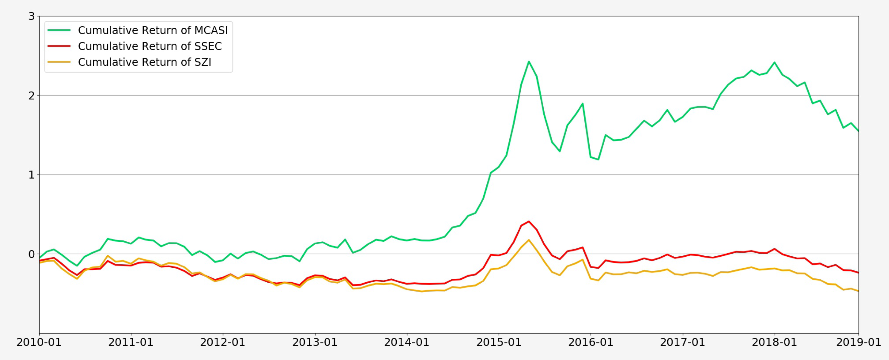
Figure 3 shows the time-series cumulative returns of all sector portfolios and MCASI. Portfolios C, I, and O have higher cumulative returns relative to MCASI, while other portfolios perform poorly relatively. At the same time, the synergy among the cumulative return curves of these portfolios is very clear and high, and the exhibited performances are mainly due to the financial crash during 2015. From 2010 to 2014, there is no obviously outstanding performance in these portfolios, and the market situation is relatively sluggish. From 2016 to 2018, there is no obvious advance for any portfolio, and all sector portfolios have been basic in the concussion period. One of the reasons for the poor performance of these portfolios during this period is that the Chinese stock market performed poorly and the Chinese financial environment was relatively unstable due to the ongoing US–China trade negotiations in 2018. Figure 3 shows that the cumulative return of portfolio B is basically maintained below the 0 scale, and investing in the mining and quarrying sector of MSCI China A-shares is not a good plan for investors.

To further analyze the high synergy shown in Figure 3, we conducted a Pearson correlation analysis for the returns of all sector portfolios.

Table 9. Correlation analysis of sector portfolios.

Correlation (%)	B	C	D	E	F	G	I	J	K	O
B	100.0 ***	75.20 ***	64.07 ***	69.24 ***	57.41 ***	72.94 ***	45.42 ***	72.72 ***	69.74 ***	53.81 ***
C	75.20 ***	100.0 ***	71.74 ***	68.95 ***	85.42 ***	70.94 ***	78.04 ***	66.77 ***	63.29 ***	83.64 ***
D	64.07 ***	71.74 ***	100.0 ***	79.42 ***	60.87 ***	77.59 ***	48.46 ***	72.59 ***	66.85 ***	60.13 ***
E	69.24 ***	68.95 ***	79.42 ***	100.0 ***	59.49 ***	77.84 ***	49.41 ***	75.90 ***	74.47 ***	56.77 ***
F	57.41 ***	85.42 ***	60.87 ***	59.49 ***	100.0 ***	59.09 ***	75.37 ***	54.45 ***	51.71 ***	77.54 ***
G	72.94 ***	70.94 ***	77.59 ***	77.84 ***	59.09 ***	100.0 ***	45.84 ***	71.20 ***	66.60 ***	65.78 ***
I	45.42 ***	78.04 ***	48.46 ***	49.41 ***	75.37 ***	45.84 ***	100.0 ***	47.75 ***	37.40 ***	82.69 ***
J	72.72 ***	66.77 ***	72.59 ***	75.9 ***	54.45 ***	71.20 ***	47.75 ***	100.0 ***	76.53 ***	52.73 ***
K	69.74 ***	63.29 ***	66.85 ***	74.47 ***	51.71 ***	66.60 ***	37.40 ***	76.53 ***	100.0 ***	48.87 ***
O	53.81 ***	83.64 ***	60.13 ***	56.77 ***	77.54 ***	65.78 ***	82.69 ***	52.73 ***	48.87 ***	100.0 ***

The statistical significance marks are in parentheses below the corresponding coefficients. *** indicates statistical significance of Pearson correlation at the 1% level. The sample period extends from January 2010 to December 2018.

shows that all correlation coefficients are statistically significant and positive, and all these values are large. Table 9 indicates that the constituents of MSCI China A-shares have a high synergy of return performance under the industry classification. Therefore, these portfolios cannot satisfy investors’ hedging needs with the condition of short-selling constraints from the hedging perspective.

Table 9 shows the correlation analysis of sector portfolios of MSCI China A-shares.

We further conducted a seasonality analysis of these sector portfolios.

Table 10. Seasonality analysis of sector portfolios.

Frequency	B	C	D	E	F	G	I	J	K	O
Panel A: Month
1	−0.26%	−1.57%	−3.82%	−2.79%	−1.00%	−1.86%	0.08%	−1.82%	−1.78%	−0.70%
2	2.14%	4.43%	1.49%	2.27%	3.08%	1.06%	7.35%	3.84%	0.52%	4.64%
3	−0.69%	2.18%	2.98%	2.18%	3.71%	1.39%	3.38%	1.04%	6.00%	2.13%
4	1.20%	0.85%	2.47%	3.50%	−0.26%	3.99%	0.84%	1.29%	1.95%	2.38%
5	−2.96%	2.73%	1.26%	−2.85%	2.36%	−1.94%	3.90%	−1.71%	−0.38%	3.66%
6	−3.67%	−2.03%	−2.41%	−3.71%	−4.67%	−3.33%	−3.03%	−3.57%	−2.07%	−1.62%
7	2.72%	2.34%	0.91%	1.65%	0.13%	0.75%	0.34%	0.96%	1.71%	1.92%
8	−1.26%	−0.35%	−0.89%	−1.37%	2.69%	0.48%	1.64%	0.07%	−1.79%	1.54%
9	0.64%	1.21%	−0.86%	−0.23%	1.78%	0.08%	3.81%	−0.32%	−1.98%	2.70%
10	2.48%	2.80%	3.48%	4.32%	2.20%	4.24%	2.59%	5.18%	3.40%	2.26%
11	−1.42%	1.08%	−0.27%	3.01%	−2.25%	0.30%	5.47%	2.61%	2.17%	3.27%
12	1.56%	1.66%	3.29%	5.50%	0.85%	1.86%	−1.63%	4.78%	6.71%	−0.93%
Panel B: Quarter
1	0.40%	1.68%	0.22%	0.55%	1.93%	0.19%	3.60%	1.02%	1.58%	2.02%
2	−1.81%	0.52%	0.44%	−1.02%	−0.86%	−0.43%	0.57%	−1.33%	−0.17%	1.47%
3	0.70%	1.07%	−0.28%	0.02%	1.53%	0.44%	1.93%	0.24%	−0.68%	2.05%
4	0.87%	1.85%	2.17%	4.28%	0.27%	2.14%	2.15%	4.19%	4.09%	1.53%
Panel C: Year
2010	0.34%	2.65%	−1.48%	1.16%	1.69%	−0.20%	2.68%	0.50%	−1.40%	3.11%
2011	−2.68%	−2.29%	−1.33%	−2.04%	−2.56%	−2.91%	−1.68%	−1.81%	0.57%	−1.97%
2012	1.18%	1.24%	1.46%	1.75%	0.71%	0.07%	−0.39%	3.68%	3.81%	0.27%
2013	−2.91%	1.91%	0.49%	−1.09%	2.23%	0.46%	5.33%	0.17%	−1.61%	2.32%
2014	2.85%	2.92%	6.58%	8.68%	2.54%	5.41%	5.57%	7.88%	6.69%	4.09%
2015	−0.00%	4.33%	1.18%	1.79%	3.61%	4.44%	8.95%	1.10%	2.57%	9.71%
2016	1.35%	0.05%	−1.28%	0.58%	−1.10%	−1.72%	−0.24%	−0.50%	−0.83%	−1.65%
2017	1.99%	3.03%	0.55%	−0.19%	1.94%	2.29%	0.39%	0.14%	2.18%	1.28%
2018	−1.75%	−2.36%	−0.44%	−2.03%	−2.59%	−2.57%	−2.03%	−1.89%	−1.14%	−1.22%

shows that the results of the monthly aggregation analysis in Panel A show that January and June have negative aggregated average returns in all portfolios, indicating that investors need to pay extra attention to these two months when making investment decisions. In February, March, April, July, October, November, and December, each sector has a better return performance than other months. Almost all sectors exhibit poor performances in June, which suggests a better investment strategy in each month in different sectors, as well as avoiding trading in June. The quarterly aggregation analysis in Panel B shows that the first and the fourth quarters have relatively better average returns, and considering the results in Panel A, the good performances of these portfolios in the first quarter are mainly caused by returns in February and March. The average monthly returns of portfolios C, I, and O are positive in all four quarters. Portfolio O has the best average return in the second quarter, but the averages of other many portfolios are negative in this quarter. Both the first and fourth quarters have positive average returns for all sectors in the MSCI of China A-shares. In Panel C, each portfolio performs well in 2014 and performs poorly in 2011 and 2018. In 2018, the Chinese stock market fluctuated more. Under such circumstances, the average monthly return loss of the portfolio D during the year is the least in all portfolios, only −0.44%. The losses of portfolios C, F and G are more serious, reaching −2.36%, −2.59%, −2.57% per month, respectively. The different losses of these sector portfolios in 2018 are directly related to the US–China trade negotiations in 2018.

Table 10 introduces seasonal analysis of sector portfolios of MSCI China A-shares, which are grouped and averaged for the months, quarters, and years. The sample period extends from January 2010 to December 2018.

In summary, among these sector portfolios, the manufacturing, information transfer, software and information technology services sectors, and sector O, have better investment attributes, such as higher returns, lower risk exposure, and larger Sharpe ratios, and the synergy of returns is high for these sector portfolios. In terms of seasonality, February, March, April, July, October, November, and December are the best months for all sector portfolios, and January and June are the worst months. The year 2018 is the bad year for all sector portfolios in the sample period.

3.3.2. Sector Return and MCASI’s Return

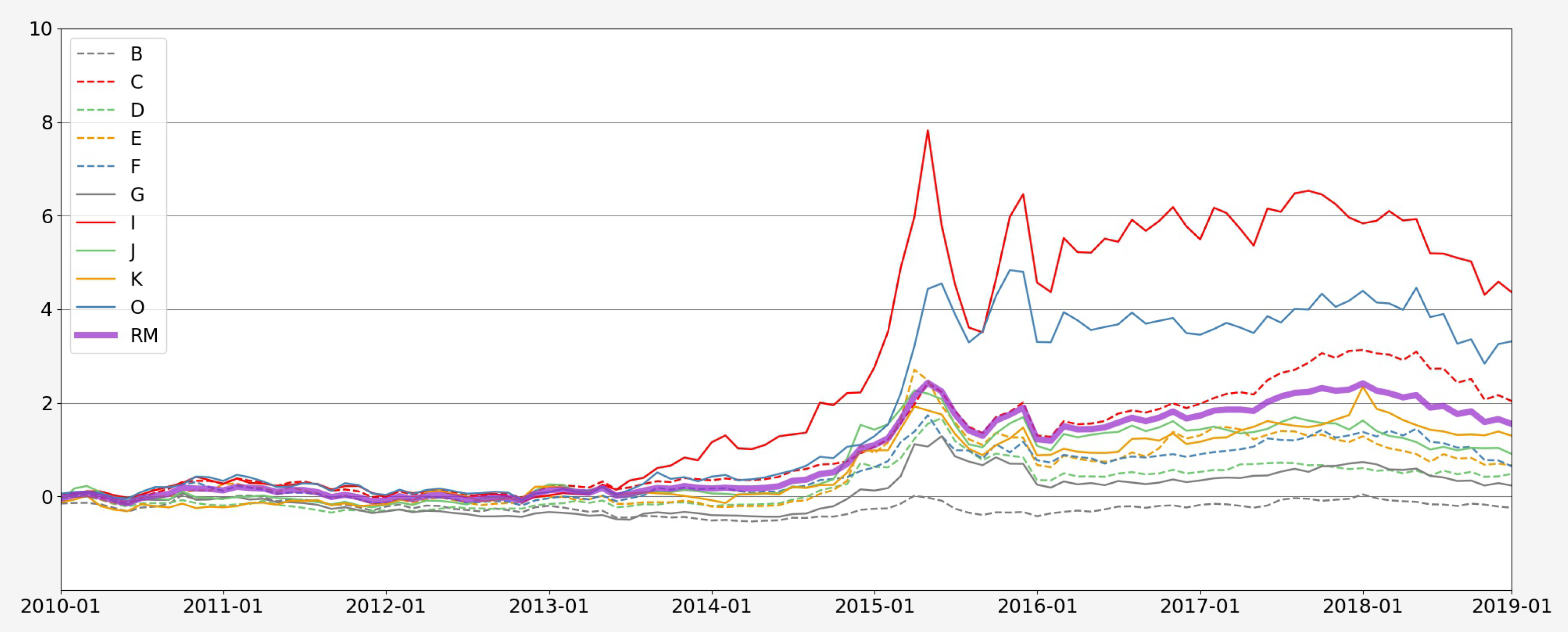
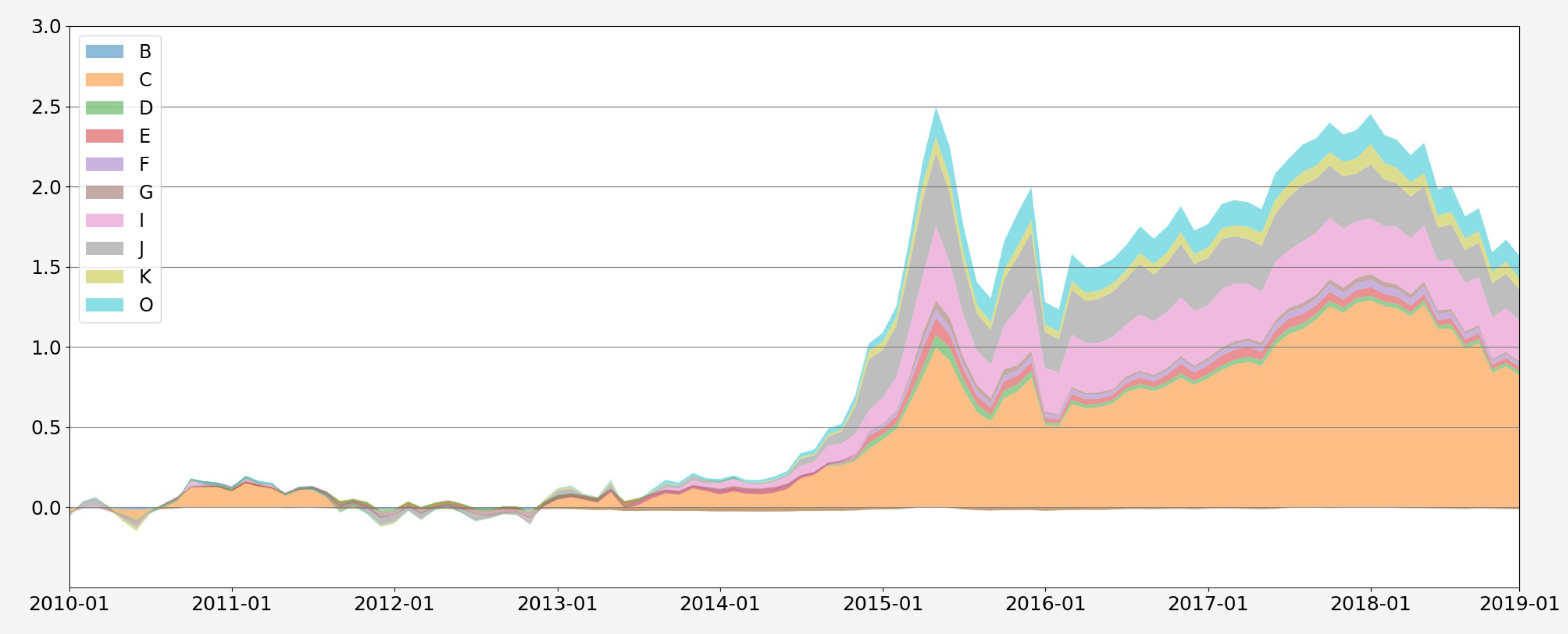
In this section, we analyze the relations between the return of the sector portfolios and MCASI’s return. First, we combined the returns of these sector portfolios with their weights and plotted the dynamic contribution of each sector portfolio to MCASI’s return in Figure 4. The weight of the return of each sector portfolio on MCASI’s return depends on the number of stocks in this sector, and the sectors’ weights on MCASI’s return are presented in Panel A of

Table 11. Forecasting MCASI’s return with the returns of the sector portfolios.

Panel A: Sector Weights on MSCI China A-Shares
$W_B$	5.08%
$W_C$	41.10%
$W_D$	5.08%
$W_E$	4.24%
$W_F$	3.39%
$W_G$	4.66%
$W_I$	5.93%
$W_J$	20.76%
$W_K$	5.51%
$W_O$	4.24%
Panel B: Results of Forecasting Regressions on MCASI’s Return
Variables	1	2	3	4	5	6	7	8	9	10	11
Intercept	0.012 *	0.011	0.011	0.010	0.011	0.011	0.009	0.010	0.011	0.010	0.013 *
$W_B*R_{B,t-1}$	3.393 **	—	—	—	—	—	—	—	—	—	4.177
$W_C*R_{C,t-1}$	—	0.167	—	—	—	—	—	—	—	—	−1.429 **
$W_D*R_{D,t-1}$	—	—	1.297	—	—	—	—	—	—	—	−6.026 *
$W_E*R_{E,t-1}$	—	—	—	3.750 **	—	—	—	—	—	—	5.294 *
$W_F*R_{F,t-1}$	—	—	—	—	2.090	—	—	—	—	—	0.147
$W_G*R_{G,t-1}$	—	—	—	—	—	3.395 **	—	—	—	—	4.657
$W_I*R_{I,t-1}$	—	—	—	—	—	—	1.894 *	—	—	—	4.906 **
$W_J*R_{J,t-1}$	—	—	—	—	—	—	—	0.710 **	—	—	0.417
$W_K*R_{K,t-1}$	—	—	—	—	—	—	—	—	1.672	—	−1.312
$W_O*R_{O,t-1}$	—	—	—	—	—	—	—	—	—	1.831	−1.488

The statistical significance marks are in parentheses below the corresponding coefficients. *, and ** indicate (2-sided) statistical significance at the 10% and 5% levels, respectively. The sample period extends from January 2010 to December 2018.

. Portfolio C (Manufacturing) has the largest weight of 41.10%, followed by portfolio J (Finance), which has a weight of 20.76%. The weights of other sector portfolios are basically around 5% with the smallest weight of 3.39% for portfolio F (wholesale and retail trades).

The relation between MCASI’s return and the sector portfolio’s return is

$$R{M}_t=\sum _{k\in S}{W}_{k}SecRe{t}_{k,t},$$

where $W_k$ denotes the weight of the sector portfolio k on MCASI’s return; $SecRe{t}_{k,t}$ is the return of the sector portfolio k for month t; S represents the set of all sector portfolios. In Figure 4, portfolio C has an absolute contribution to MCASI’s return, followed by the portfolio J, and portfolios I and O also have some contribution. Compared with portfolios C and J, which have high contributions on MCASI’s return caused by their high weights, portfolios I and J have high contributions due to their respective high returns. Therefore, from the investment perspective, and regarding MCASI’s return with higher investment weights in portfolio I, J will perform better, and investors need to pay more attention to sectors I and J.

Since MCASI’s return constructed by all constituents belongs to different sectors, do the sector portfolios have predictive effects on MCASI’s return? In order to answer this question, we use the sector-weighted returns of sector portfolios to predict the future MCASI returns. First, we conducted a univariate analysis to simply judge the effect of the returns of a single sector portfolio on MCASI’s return. Then, we conducted a multivariate analysis using the returns of all sector portfolios to forecast the future MCASI returns.

Table 11 introduces the coefficients of the regressions for forecasting MCASI’s return with returns of sector portfolios. Panel A presents the weights of these sectors of MSCI China A-shares, which were calculated according to the number of stocks in each sector. Panel B shows the specific results of regressions, where $R_{i,t}$ indicates the return of sector portfolio i for month t.

Panel B of Table 11 introduces the specific results of all regressions. For the univariate regressions, the returns of portfolios B, E, G, I, and J all have a significantly positive impact on MCASI’s return. For the multivariate regression of the last column of Panel B, the returns of portfolios C and D become significant and have a negative impact on the future MCASI return while they are insignificant for the results of the univariate regressions. The returns of portfolios E and I remain significant and have positive impact on the future MCASI return in the multivariate regression results. Due to the high synergy between sector portfolios which is showed in the correlation analysis of Table 9 and Figure 3, there may be multicollinearity in the multivariate regression to make the coefficients of these variables unreliable. However, considering the results of both univariate and multivariate models, we also conclude that the return of the sector construction and the return of the sector of information transfer, software and information technology services have significant and positive effects on the future MCASI return.

3.3.3. Portfolio Analysis for Sectors

Investors are interested in how to allocate cash among different sectors to ensure lower risk exposure or a larger Sharpe ratio. In this section, we provide various types of portfolio analyses for the sector return of MSCI China A-shares.

The first type of portfolio is just concerned with MCASI’s return (RM), mentioned above, which serves as our benchmark. The second one is an equal-weighted portfolio (EWP) for these sector returns, and the third one is return-weighted portfolio (RWP), which focuses on the past returns of sectors. Specifically, for the next period, RWP allocates the cash weight of each sector to

$${\omega }_{k,t}=\frac{AE{R}_{k,t-1}}{{\sum }_{j=1}^{10}AE{R}_{j,t-1}},$$

where

$$AE{R}_{k,t-1}=\left\{\begin{array}{cc}0\hfill & \mathrm{if}\frac{1}{36}\sum _{i=1}^{36}(SecRe{t}_{k,t-i}-R{F}_{t-i})<0,\hfill \\ \frac{1}{36}\sum _{i=1}^{36}(SecRe{t}_{k,t-i}-R{F}_{t-i})\hfill & \mathrm{else},\hfill \end{array}\right.$$

is the average excess return of sector k over the past 36 months for month $t-1$. The condition that the average excess return is greater than zero is due to the short-selling constraints in the Chinese stock market.

The fourth portfolio is the Sharpe ratio-weighted portfolio (SRWP), and the weight for each sector is

$${\omega }_{k,t}=\frac{AE{R}_{k,t-1}}{{\sigma }_{k,t-1}}·\frac{1}{{\sum }_{j=1}^{10}\frac{AE{R}_{k,t-1}}{{\sigma }_{k,t-1}}},$$

where $AE{R}_{k,t-1}$ is the same definition as above and ${\sigma }_{k,t-1}$ is the standard deviation of monthly returns over the past 36 months for sector k in month $t-1$.

The fifth portfolio is a volatility-weighted portfolio (VWP), the weight of which is calculated by

$${\omega }_{k,t}=\frac{1}{{\sigma }_{k,t-1}}·\frac{1}{{\sum }_{j=1}^{10}\frac{1}{{\sigma }_{k,t-1}}},$$

where ${\sigma }_{k,t-1}$ is the same definition as above. The fifth portfolio type is just a rough way to avoid risks without considering the covariance among sectors’ returns. So, the sixth is the minimum-variance portfolio (MVP) according to Markowitz (1952) with the goal of minimizing portfolio risk exposure, and the weights of sectors need to solve a quadratic programming as

$$\begin{array}{cc}\hfill minimiz{e}_{\{{\omega }_1,{\omega }_2,\cdots ,{\omega }_{10}\}}& {\sigma }_{r_p}=\sum _{i=1}^{10}\sum _{j=1}^{10}{\omega }_i{\omega }_{j}cov(r_i,r_j)\hfill \\ \hfill subjectto& r_p=\sum _{i=1}^{10}{\omega }_i{r}_i,\hfill \\ & \sum _{i=1}^{10}{\omega }_i=1,{\omega }_i\ge 0,i\in 1,2,\cdots ,10,\hfill \end{array}$$

where the condition of ${\omega }_i\ge 0$ is due to the same reason of short-selling constraints as RWP. We use sectors’ returns over the past 36 months to solve the quadratic programming and obtain the optimal weights for any month t.

Considering the dynamic mean and volatility for the sectors’ returns, the last portfolio type is the AR-GARCH minimum-variance portfolio (AGMVP). Based on Hu et al. (2019), we used the AR(1)-GARCH(1,1) model for each sector portfolio’s time-series returns instead of ARMA-GARCH models in Hu et al. (2019), where they fit ARMA(1,1)-GARCH(1,1) for the returns of crypto assets. Then, we also approached the joint distribution of the sample innovations from AR(1)-GARCH(1,1) models by the multivariate Copula method, where the Copula function is based on the multivariate normal distribution. For each one-step forecast, we generated 1000 joint sample innovations and calculated 1000 simulated returns for each sector based on the coefficients of the AR-GARCH models. Then, we followed MVP’s procedure to obtain the optimal weights with the simulated returns. The initial 36 observations were utilized to generate the first one-step optimal sector weights and each of the next optimal sector weights, and, consistent with the constructed portfolios above, we used the recent 36 observations to fit the AR-GARCH models.

Our sample period extends from January 2010 to December 2018, and the observation period of our six portfolios is from January 2013 to December 2018, and we used the previous 36 data to compute related measures.

Table 12. Sector portfolios of MSCI China A-shares.

	RM	EWP	RWP	VWP	SRWP	MVP	AGMVP
Observations	72	72	72	72	72	72	72
Mean (%)	1.49	1.47	1.52	1.51	1.57	1.90	1.71
Minimum (%)	−23.27	−23.21	−24.56	−22.76	−24.32	−23.56	−23.39
Maximum (%)	19.42	24.13	24.06	23.18	23.29	27.21	20.00
Standard Deviation (%)	7.27	7.65	8.03	7.56	7.95	7.58	7.59
Skewness	−0.26	0.13	0.10	0.10	0.07	−0.04	−0.47
Kurtosis	1.98	2.37	1.96	2.29	1.95	2.59	1.64
Annualized Return (%)	23.44	22.32	22.71	23.53	24.32	36.22	29.29
Sharpe Ratio	0.63	0.59	0.58	0.61	0.61	0.79	0.70
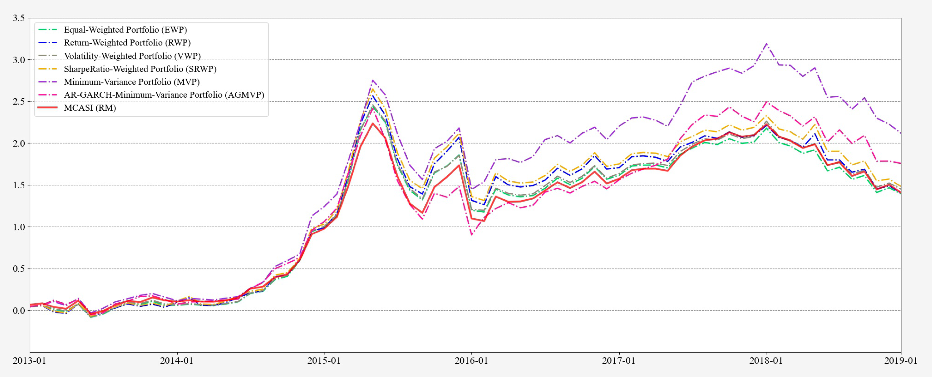
Maximum Drawdown (%)	−36.11	−37.54	−38.02	−37.07	−37.78	−34.06	−44.33

shows the information of these seven portfolios. We refreshed our portfolios’ weights every month and there are 72 observations to compare these portfolios’ performances. MVP has the highest average of 1.9% and maximum of 27.21% for monthly returns, and the corresponding values for MCASI (RM) are the lowest, at 1.49% and 19.42%. All portfolios have approximate minimums in their monthly returns. MVP has the highest annualized return of 36.22%, followed by AGMVP, which has the annualized return of 29.29%. The results of the Sharpe ratio also show that the MVP exhibits the best performance in our sample. In terms of a risk measure worthy of investors’ attention, the maximum drawdown results suggest that MVP has an advantage among the seven portfolios, and the AGMVP performs poorly. EWP, RWP, VWP and SRWP are not particularly prominent compared to MCASI in almost all respects. Figure 5 also shows the cumulative return curves for all six portfolios, and MVP has an obvious advantage in terms of performance.

Table 12 introduces portfolios’ information for sector return of MSCI China A-shares. These portfolios are described in the text, including the basic portfolio with respect to MCASI’s return (RM), equal-weighted portfolio (EWP), return-weighted portfolio (RWP), volatility-weighted portfolio (VWP), Sharpe ratio-weighted portfolio (SRWP), minimum-variance portfolio (MVP), and AR-GARCH-minimum-variance portfolio (AGMVP). Our sample period extends from January 2010 to December 2018, and the observation period of our six portfolios is from January 2013 to December 2018 considering we used the previous 36 data to compute related measures.

Investors can use the classic Markowitz portfolio approach to allocate their money in these sectors of MSCI China A-shares and achieve a better investment performance in terms of average return, standard deviation, annualized return, the Sharpe ratio, and maximum drawdown.

4. Conclusions

We studied 236 stocks of China A-shares in the MSCI Emerging Market Index published by MSCI in August 2018. We introduced the MSCI China A-shares index (MCASI) and analyzed the properties of MCASI in the Chinese stock market from the return, volatility, sentiment, and liquidity perspectives. Moreover, over the sample period, MCASI advantageously outperformed other indexes, SSEC and SZI, in the Chinese stock market. We analyzed whether MCASI’s investor sentiment, liquidity, and volatility have impacts on forecasting MCASI’s return, and the results show that MCASI’s investor sentiments, both overnight sentiment and BW sentiment, are more important for MCASI’s return. From the perspective of sector investment, we present basic performance statistics, a correlation, and seasonality analysis for 10 sector portfolios. Specifically, the sector portfolio of information transfer, software and information technology services performs better in the sample period and has the largest monthly average return of 2.06%. We also examine seven approaches of the optimal portfolio in sectors, and the classic Markowitz portfolio approach (MVP) is recommended. Our empirical analysis would be helpful for domestic and foreign investors to form investment strategies in MSCI China A-shares.

References

1. Aboody, David, Omri Even-Tov, Reuven Lehavy, and Brett Trueman. 2018. Overnight returns and firm-specific investor sentiment. Journal of Financial and Quantitative Analysis 53: 485–505. [Google Scholar] [CrossRef] [Green Version]
2. Amihud, Yakov. 2002. Illiquidity and stock returns: Cross-section and time-series effects. Journal of Financial Markets 5: 31–56. [Google Scholar] [CrossRef] [Green Version]
3. Asquith, Paul, and David W. Mullins Jr. 1986. Equity issues and offering dilution. Journal of Financial Economics 15: 61–89. [Google Scholar] [CrossRef]
4. Audrino, Francesco, Fabio Sigrist, and Daniele Ballinari. 2019. The impact of sentiment and attention measures on stock market volatility. International Journal of Forecasting 36: 334–57. [Google Scholar] [CrossRef]
5. Baker, Malcolm, and Jeffrey Wurgler. 2002. Market timing and capital structure. The Journal of Finance 57: 1–32. [Google Scholar] [CrossRef]
6. Baker, Malcolm, and Jeffrey Wurgler. 2006. Investor sentiment and the cross-section of stock returns. The Journal of Finance 61: 1645–80. [Google Scholar] [CrossRef] [Green Version]
7. Baker, Malcolm, Jeffrey Wurgler, and Yu Yuan. 2012. Global, local, and contagious investor sentiment. Journal of Financial Economics 104: 272–87. [Google Scholar] [CrossRef] [Green Version]
8. Barardehi, Yashar H., Dan Bernhardt, and Ryan J. Davies. 2018. Trade-time measures of liquidity. The Review of Financial Studies 32: 126–79. [Google Scholar] [CrossRef] [Green Version]
9. Berkman, Henk, Paul D. Koch, Laura Tuttle, and Ying Jenny Zhang. 2012. Paying attention: Overnight returns and the hidden cost of buying at the open. Journal of Financial and Quantitative Analysis 47: 715–41. [Google Scholar] [CrossRef]
10. Chakrabarti, Rajesh, Wei Huang, Narayanan Jayaraman, and Jinsoo Lee. 2005. Price and volume effects of changes in MSCI indices–nature and causes. Journal of Banking and Finance 29: 1237–64. [Google Scholar] [CrossRef] [Green Version]
11. Chen, Hung-Ling, Cheng-Yi Shiu, and Hui-Shan Wei. 2019. Price effect and investor awareness: Evidence from MSCI Standard Index reconstitutions. Journal of Empirical Finance 50: 93–112. [Google Scholar] [CrossRef]
12. Chowdhury, Anup, Moshfique Uddin, and Keith Anderson. 2018. Liquidity and macroeconomic management in emerging markets. Emerging Markets Review 34: 1–24. [Google Scholar] [CrossRef]
13. Clark, Todd E., and Kenneth D. West. 2007. Approximately normal tests for equal predictive accuracy in nested models. Journal of Econometrics 138: 291–311. [Google Scholar] [CrossRef] [Green Version]
14. Da, Zhi, Joseph Engelberg, and Pengjie Gao. 2014. The sum of all FEARS investor sentiment and asset prices. The Review of Financial Studies 28: 1–32. [Google Scholar] [CrossRef] [Green Version]
15. Gao, Lu, and Lian Chen. 2017. Market impact analysis of China A-shares into MSCI index–comparison of volatility between MSCI China international index and CSI 300 index. In Second International Conference On Economic and Business Management (FEBM 2017). Paris: Atlantis Press. [Google Scholar]
16. Hau, Harald, Massimo Massa, and Joel Peress. 2009. Do demand curves for currencies slope down? Evidence from the MSCI global index change. The Review of Financial Studies 23: 1681–717. [Google Scholar] [CrossRef]
17. Hu, Yuan, Svetlozar T. Rache, and Frank J. Fabozzi. 2019. Modelling Crypto Asset Price Dynamics, Optimal Crypto Portfolio, and Crypto Option Valuation. arXiv arXiv:1908.05419. [Google Scholar]
18. Hung, Chung-Wen, and Cheng-Yi Shiu. 2016. Trader activities, ownership, and stock price reactions to MSCI standard index changes: Evidence from Taiwan. Journal of Multinational Financial Management 36: 49–63. [Google Scholar] [CrossRef]
19. Joseph, Kissan, M. Babajide Wintoki, and Zelin Zhang. 2011. Forecasting abnormal stock returns and trading volume using investor sentiment: Evidence from online search. International Journal of Forecasting 27: 1116–27. [Google Scholar] [CrossRef]
20. Lee, Bong Soo, Miyoun Paek, Yeonjeong Ha, and Kwangsoo Ko. 2015. The dynamics of market volatility, market return, and equity fund flow: International evidence. International Review of Economics and Finance 35: 214–27. [Google Scholar] [CrossRef]
21. Leuz, Christian, Karl V. Lins, and Francis E. Warnock. 2008. Do foreigners invest less in poorly governed firms? The Review of Financial Studies 22: 3245–85. [Google Scholar] [CrossRef]
22. Li, Yan, and Weiping Li. 2021. Firm-specific investor sentiment for the chinese stock market. Economic Modelling 97: 231–46. [Google Scholar] [CrossRef]
23. Liu, Shuming. 2015. Investor sentiment and stock market liquidity. Journal of Behavioral Finance 16: 51–67. [Google Scholar] [CrossRef]
24. Loughran, Tim, and Jay R. Ritter. 1995. The new issues puzzle. The Journal of Finance 50: 23–51. [Google Scholar] [CrossRef]
25. Loughran, Tim, and Jay R. Ritter. 1997. The operating performance of firms conducting seasoned equity offerings. The Journal of Finance 52: 1823–50. [Google Scholar] [CrossRef]
26. Ma, Rui, Hamish D. Anderson, and Ben R. Marshall. 2018. Market volatility, liquidity shocks, and stock returns: Worldwide evidence. Pacific-Basin Finance Journal 49: 164–99. [Google Scholar] [CrossRef]
27. Markowitz, Harry. 1952. Portfolio selection. The Journal of Finance 7: 77–91. [Google Scholar]
28. Masulis, Ronald W., and Ashok N. Korwar. 1986. Seasoned equity offerings: An empirical investigation. Journal of Financial Economics 15: 91–118. [Google Scholar] [CrossRef]
Figure 1. Variables’ Time-Series Charts of MSCI China A-shares. Notes: Figure 1 presents time-series charts of our variables. FundCR refers to mutual fund premium rate. Turnover denotes MCASI’s turnover which is equal-weight turnover average of all stocks in MCASI. SEO represents SEOs initial return. S e n t O N and S e n t B W are MCASI’s overnight sentiment and BW sentiment, respectively. Price impact and Trade-time liquidity are MCASI’s liquidity measures. RV refers to MCASI’s volatility which is the aggregation of the standard deviation of daily returns of all stocks in MCASI for a given month. FundCR, Turnover and SEO are three components of MCASI’s BW sentiment. All variables are described in the text. The sample period extends from January 2010 to December 2018.
Jrfm 14 00514 g001
Figure 2. Cumulative Return of MCASI. Notes: Figure 2 presents cumulative returns of MCASI, SSEC and SZI in our sample period. SSEC and SZI stand for Shanghai Composite Index and Shenzhen Component Index, respectively. The sample period extends from January 2010 to December 2018.
Jrfm 14 00514 g002
Figure 3. MCASI’s return and sector portfolio’s return. Notes: Figure 3 produces time-series charts of the cumulative returns of the sector portfolios. The tags and full names of these sector portfolios can be found in Panel A of Table 8. MCASI’s return of R M is described in the Variable Definitions section. The sample period extends from January 2010 to December 2018.
Jrfm 14 00514 g003
Figure 4. Sectors’ contributions to MCASI’s return. Notes: Figure 4 introduces the contribution of the returns of the sector portfolios on MCASI’s return. The tags and full names of these sector portfolios can be found in Panel A of Table 8. The weights of the returns of the sector portfolios on MCASI’s return are presented in Panel A of Table 11. The relation between MCASI’s return and the sector portfolio’s return is R M t = k S W k S e c R e t k , t , where W k is the weight of the sector portfolio k on MCASI’s return; S e c R e t k , t is the return of the sector portfolio k for month t; S is the set of all sector portfolios. The sample period extends from January 2010 to December 2018.
Jrfm 14 00514 g004
Figure 5. Various types of portfolios for sector return. Notes: Figure 5 introduces the cumulative returns of various types of portfolios for sector return. These portfolios are described in the text, including MCASI (RM), equal-weighted portfolio (EWP), return-weighted portfolio (RWP), volatility-weighted portfolio (VWP), Sharpe ratio-weighted (SRWP), minimum-variance portfolio (MVP), and AR-GARCH-minimum-variance portfolio (AGMVP). The observation period of six portfolios is from January 2013 to December 2018 considering that we used the previous 36 data to compute related measures.
Jrfm 14 00514 g005